A Multi-Urn Model for Network Search

Christopher E MarksOperations Research Center, Massachusetts Institute of Technology

Charles Stark Draper Laboratory

555 Technology SquareCambridge, MA 02139

cemarks@mit.edu

Tauhid ZamanDepartment of Operations Management, Sloan School of Management

Massachusetts Institute of Technology

77 Massachusetts Ave.Cambridge, MA 02139

zlisto@mit.edu

We consider the problem of finding a specific target individual hiding in a social network. We propose a

method for network vertex search that looks for the target vertex by sequentially examining the neighbors of

a set of “known” vertices to which the target vertex may have connected. The objective is to find the target

vertex as quickly as possible from amongst the neighbors of the known vertices. We model this type of search

as successively drawing marbles from a set of urns, where each urn represents one of the known vertices

and the marbles in each urn represent the respective vertex’s neighbors. Using a dynamic programming

approach, we analyze this model and show that there is always an optimal “block” policy, in which all of

the neighbors of a known vertex are examined before moving on to another vertex. Surprisingly, this block

policy result holds for arbitrary dependencies in the connection probabilities of the target vertex and known

vertices. Furthermore, we give precise characterizations of the optimal block policy in two specific cases:

(1) when the connections between the known vertices and the target vertex are independent, and (2) when

the target vertex is connected to at most one known vertex. Finally, we provide some general monotonicity

properties and discuss the relevance of our findings in social media and other applications.

1. Introduction

In this paper, we examine the problem of searching a social network for a particular target indi-

vidual by sequentially examining the neighbors of other known users. Social media applications

enable users to connect with each other, forming social networks. For different reasons which we

will discuss, one may wish to find a target individual in the social network. One may have prior

knowledge that the target individual is connected with a set of known users, and so the most logical

place to begin searching is the neighbors of these known users. If querying each of these neighbors

incurs some sort of cost, then the goal would be to find the target with as few queries as possible.

1

arX

iv:1

608.

0808

0v1

[m

ath.

OC

] 2

4 A

ug 2

016

Marks and Zaman: Multi-Urn Model for Network Search2

For example, suppose Mary is searching a social media application for an account belonging

to John, an old friend from school with whom she has lost contact. From what she knows about

John, Mary might be able to develop a list of accounts she knows about within the social media

application to which John’s account might be connected. For example, she might recall that John

was good friends with Matt, who has a social media account that is known to Mary. She also might

remember John was active in a certain charity, which also maintains a social media account known

to Mary.

After developing such a list, Mary could sequentially explore each account’s connections, but

doing so could take a substantial amount of time. In order to find John’s account quickly (assuming

John has an account), Mary might devise a search strategy. For example, she might start by looking

at accounts she feels are the most likely to be connected with John’s account. Alternatively, she

might start by looking at accounts with fewer connections, because her goal is to find John’s

account while minimizing the time spent exploring.

In this hypothetical scenario, what Mary is doing is an example of a network vertex search

in which the sought object, or target might be found by examining the neighbors of a finite set

of known vertices. Once the search target is found, the search typically terminates. Each known

vertex i might have a different degree, Ni, requiring a different number of search queries to exhaus-

tively search. From our scenario, we also consider that each known vertex i might have a different

probability of being connected to the target vertex, which we denote as ϕi.

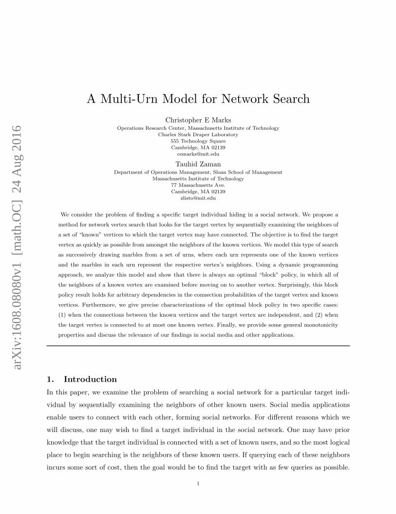
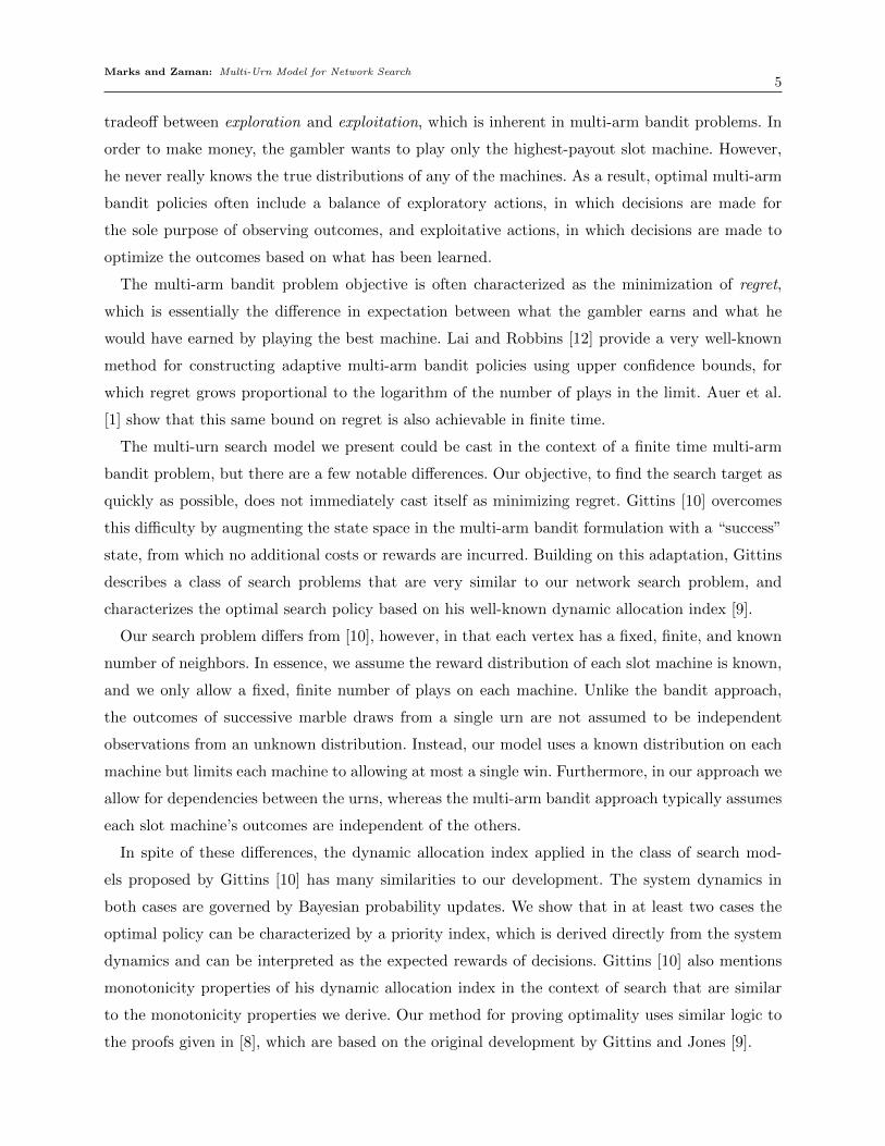
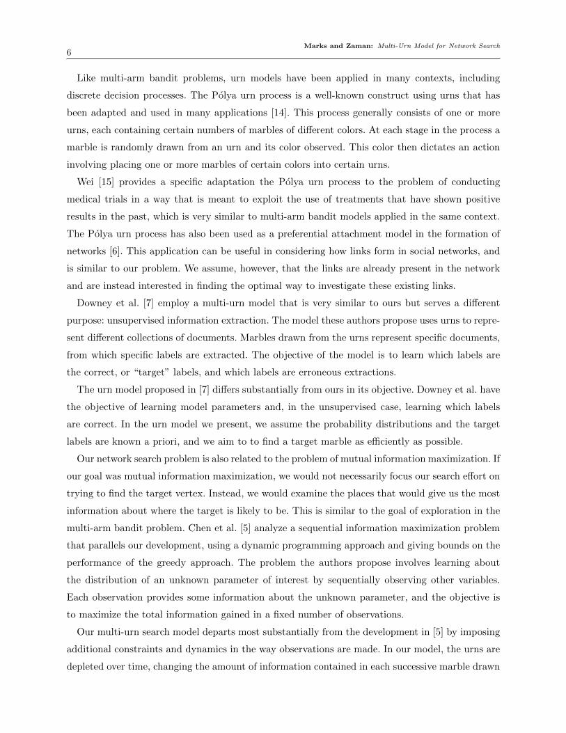
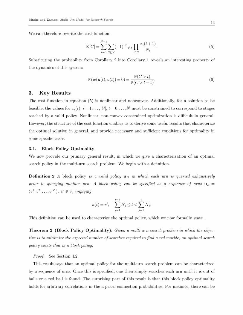
In this paper we present a probabilistic “multi-urn” model for searches of this nature in which

we represent each known vertex as an urn containing a finite number of marbles. Each marble

in an urn represents one of the respective vertex’s neighbors. The search consists of successively

drawing and and examining individual marbles from the urns with the goal of finding a red marble,

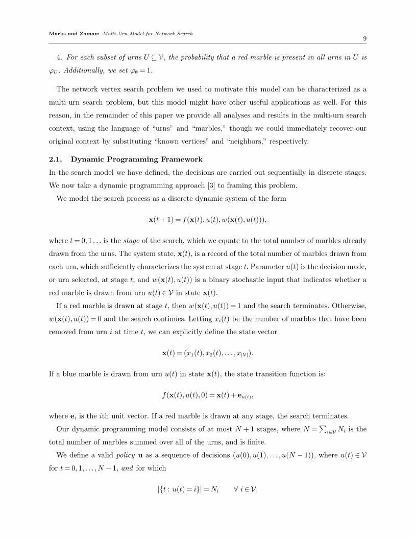
representing the search target, in the fewest number of draws. Figure 1 depicts the multi-urn

model for a network search on three known vertices. In this example, each of the known vertices

is connected to the search target, so each urn contains a single red marble. Additionally, each urn

contains a number of blue marbles that represent the other neighbors belonging to each respective

vertex. Employing a dynamic programming framework, we provide some insight into the optimal

search policy in this general model and under certain conditions.

1.1. Application

Our model applies to any scenario where one must sequentially search for the target amongst a

set of entities which are separated into different clusters. In our vertex search problem, the entities

are vertices and the clusters are neighborhoods of the known vertices. Our main motivation for

this model is in social media applications where many times the goal is to find users who harass

Marks and Zaman: Multi-Urn Model for Network Search3

AB

C

A

B

CTarget

NA=3

NB=2

NC=3

Figure 1 Network search representation as a multi-urn model.

others, incite violence, or engage in other dangerous behaviors. Twitter has been suspending large

numbers of users, many of which support or engage in violent extremism, from its micro-blogging

application for violating the site’s published rules [11]. The challenge is that these users can simply

create a new account each time one is suspended. However, from historical data Twitter could

predict the accounts to which the suspended user is likely to connect. Using this information,

Twitter administrators could then apply our optimality criteria to efficiently locate new accounts

belonging to suspended users.

There are other scenarios where this model can apply. For instance, for law enforcement and

intelligence applications, the search entities could be suspects in a crime and the clusters could be

geographical locations. Or if one is examining a dump of emails from a suspect’s server, one may

be looking for an incriminating email, so the entities are emails and the clusters could be recipients

of the emails. In both of these examples, the process of querying the entities requires a non-trivial

amount of resources (interviewing a suspect, reading an email), so it is important to find the target

as quickly as possible. Using an optimal or near-optimal search strategy is therefore crucial in these

examples.

1.2. Our Contributions

In this paper we develop a multi-urn search model, a new and useful methodology for analyzing

searches similar to the network vertex search problem we proposed in the introduction. We employ

a dynamic programming framework to analyze this model and provide theoretical results based on

the nature of the cost function.

In particular, we show that in this type of search problem there always exists an optimal policy,

i.e., one that minimizes the expected number of marbles drawn before finding a red marble, in

which the marbles in each urn are exhausted before moving on to the next urn (Theorem 2).

Marks and Zaman: Multi-Urn Model for Network Search4

We refer to a policy that meets this criterion as a block policy, and show that this result holds

irrespective of dependencies among the urns. This result is surprising because the presence of the

red ball in the urns could have arbitrary correlations. There could be positive correlations, where if

the ball is in one urn, it is more likely to be in another urn. Or the correlations could be negative,

so if a ball is in one urn, it is less likely to be in another urn. Nonetheless, our result shows that

no matter what the dependency between the urns, a block policy is always an optimal policy to

find the red ball.

Building on this finding, we provide optimality conditions that enable immediate determination

of an optimal policy in two specific cases:

• Each urn contains a red marble independent of other urns (Theorem 4). This case corresponds

to the assumption that each known vertex is connected to the search target independent of other

known vertices’ connections.

• There is at most one red marble among all of the urns (Theorem 6). This case corresponds to

the assumption that the search target is connected to at most one known vertex.

Finally, we provide detailed analysis of the system dynamics of the multi-urn search model,

leading to insight into the intuition behind our findings. We provide monotonicity properties on

the evolution of certain probabilities as marbles are successively drawn (Theorem 7) and establish

a useful bound on how much the probability of drawing a red marble from a certain urn can change

between two successive stages (Theorem 8).

1.3. Previous Work

Much of the work that has been done in the context of network search is focused on finding relevant

vertices in a large scale network. Google’s PageRank algorithm is probably the most well known

example of these methods, of which many adaptations and generalizations exist [2]. Our work looks

at an essentially different type of network search: one of finding a specific vertex in a network,

presumably identifiable by certain features, by investigating network neighborhoods in which the

vertex is likely to appear.

The network vertex search problem we have proposed could instead be formulated as a multi-arm

bandit problem. Bubeck and Cesa-Bianchi [4] provide a broad survey of many variations of the

multi-arm bandit problem and their respective applications. These problems are typically likened

to a gambler who has a choice of playing from a set of slot machines. At each discrete stage in the

process the gambler selects and plays a slot machine for a certain cost and receives a stochastic

reward from an unknown distribution. The more times the gambler plays a particular machine, the

more he is able to learn about its reward distribution.

In the multi-arm bandit setting, the gambler would not want to spend too much money playing

low-payout slot machines just to learn their reward distribution. This quandary is the fundamental

Marks and Zaman: Multi-Urn Model for Network Search5

tradeoff between exploration and exploitation, which is inherent in multi-arm bandit problems. In

order to make money, the gambler wants to play only the highest-payout slot machine. However,

he never really knows the true distributions of any of the machines. As a result, optimal multi-arm

bandit policies often include a balance of exploratory actions, in which decisions are made for

the sole purpose of observing outcomes, and exploitative actions, in which decisions are made to

optimize the outcomes based on what has been learned.

The multi-arm bandit problem objective is often characterized as the minimization of regret,

which is essentially the difference in expectation between what the gambler earns and what he

would have earned by playing the best machine. Lai and Robbins [12] provide a very well-known

method for constructing adaptive multi-arm bandit policies using upper confidence bounds, for

which regret grows proportional to the logarithm of the number of plays in the limit. Auer et al.

[1] show that this same bound on regret is also achievable in finite time.

The multi-urn search model we present could be cast in the context of a finite time multi-arm

bandit problem, but there are a few notable differences. Our objective, to find the search target as

quickly as possible, does not immediately cast itself as minimizing regret. Gittins [10] overcomes

this difficulty by augmenting the state space in the multi-arm bandit formulation with a “success”

state, from which no additional costs or rewards are incurred. Building on this adaptation, Gittins

describes a class of search problems that are very similar to our network search problem, and

characterizes the optimal search policy based on his well-known dynamic allocation index [9].

Our search problem differs from [10], however, in that each vertex has a fixed, finite, and known

number of neighbors. In essence, we assume the reward distribution of each slot machine is known,

and we only allow a fixed, finite number of plays on each machine. Unlike the bandit approach,

the outcomes of successive marble draws from a single urn are not assumed to be independent

observations from an unknown distribution. Instead, our model uses a known distribution on each

machine but limits each machine to allowing at most a single win. Furthermore, in our approach we

allow for dependencies between the urns, whereas the multi-arm bandit approach typically assumes

each slot machine’s outcomes are independent of the others.

In spite of these differences, the dynamic allocation index applied in the class of search mod-

els proposed by Gittins [10] has many similarities to our development. The system dynamics in

both cases are governed by Bayesian probability updates. We show that in at least two cases the

optimal policy can be characterized by a priority index, which is derived directly from the system

dynamics and can be interpreted as the expected rewards of decisions. Gittins [10] also mentions

monotonicity properties of his dynamic allocation index in the context of search that are similar

to the monotonicity properties we derive. Our method for proving optimality uses similar logic to

the proofs given in [8], which are based on the original development by Gittins and Jones [9].

Marks and Zaman: Multi-Urn Model for Network Search6

Like multi-arm bandit problems, urn models have been applied in many contexts, including

discrete decision processes. The Polya urn process is a well-known construct using urns that has

been adapted and used in many applications [14]. This process generally consists of one or more

urns, each containing certain numbers of marbles of different colors. At each stage in the process a

marble is randomly drawn from an urn and its color observed. This color then dictates an action

involving placing one or more marbles of certain colors into certain urns.

Wei [15] provides a specific adaptation the Polya urn process to the problem of conducting

medical trials in a way that is meant to exploit the use of treatments that have shown positive

results in the past, which is very similar to multi-arm bandit models applied in the same context.

The Polya urn process has also been used as a preferential attachment model in the formation of

networks [6]. This application can be useful in considering how links form in social networks, and

is similar to our problem. We assume, however, that the links are already present in the network

and are instead interested in finding the optimal way to investigate these existing links.

Downey et al. [7] employ a multi-urn model that is very similar to ours but serves a different

purpose: unsupervised information extraction. The model these authors propose uses urns to repre-

sent different collections of documents. Marbles drawn from the urns represent specific documents,

from which specific labels are extracted. The objective of the model is to learn which labels are

the correct, or “target” labels, and which labels are erroneous extractions.

The urn model proposed in [7] differs substantially from ours in its objective. Downey et al. have

the objective of learning model parameters and, in the unsupervised case, learning which labels

are correct. In the urn model we present, we assume the probability distributions and the target

labels are known a priori, and we aim to to find a target marble as efficiently as possible.

Our network search problem is also related to the problem of mutual information maximization. If

our goal was mutual information maximization, we would not necessarily focus our search effort on

trying to find the target vertex. Instead, we would examine the places that would give us the most

information about where the target is likely to be. This is similar to the goal of exploration in the

multi-arm bandit problem. Chen et al. [5] analyze a sequential information maximization problem

that parallels our development, using a dynamic programming approach and giving bounds on the

performance of the greedy approach. The problem the authors propose involves learning about

the distribution of an unknown parameter of interest by sequentially observing other variables.

Each observation provides some information about the unknown parameter, and the objective is

to maximize the total information gained in a fixed number of observations.

Our multi-urn search model departs most substantially from the development in [5] by imposing

additional constraints and dynamics in the way observations are made. In our model, the urns are

depleted over time, changing the amount of information contained in each successive marble drawn

Marks and Zaman: Multi-Urn Model for Network Search7

in predictable, but sometimes unintuitive ways. Our main contributions are the characterizations

of optimal search policies under various probability models, which come directly from analysis of

the dynamics inherent in our multi-urn search model.

Finally, recent work in scheduling and inspection policies employ similar dynamic programming

approaches to characterize optimal policies. Levi et al. [13] use dynamic programming to find

policies that optimally allocate resources between information gathering and task execution. This

class of models provides a natural extension to our network search problem. While we assume a

probability model on a set of known vertices, using this approach we could attempt to find the

optimal balance between the time spent learning a probability model on a set of known vertices

and the time spent executing the search on the current known vertex set.

2. Multi-urn Search Model

We return to the context of network vertex search as presented in the introduction. Let V be the

set of vertices to search, and let Ni be the number of search queries required to exhaustively search

vertex i ∈ V. We assume that the neighbors of each vertex are queried in a random order, so that

each individual neighbor query of a particular vertex is equally likely to be the search target, given

that the target is connected to the queried vertex.

Under these assumptions, we can represent this search problem as an experiment involving

randomly drawing marbles from a set of urns, where each urn represents a known vertex in the

network. Each marble in urn i ∈ V represents a neighbor of vertex i. The degree of vertex i is Ni,

so urn i initially has Ni marbles. With probability ϕi > 0, exactly one of the Ni marbles in urn i

is red, indicating that known vertex i is connected to the target vertex. Otherwise, all marbles in

all urns are blue.

Querying a random neighbor of vertex i in search of the target is analogous to drawing a random

marble from urn i and observing its color. If the marble is red, the target vertex has been located.

If the marble is blue, the target has not been found and the search continues with the remaining

marbles. Note that blue marbles are not put back into the urns; once they are drawn they are

discarded. Just as Mary desires to find her old friend John with as few searches as possible, the

goal in this experiment is to minimize the number of blue marbles drawn before finding a red one.

We now more completely specify the probability model that accounts for how the target vertex

might be connected to the set of known vertices, i.e., how red marbles might be distributed among

the urns. Let Ai be the event that the target vertex is connected to vertex i. We have already

defined

ϕi = P(Ai).

Marks and Zaman: Multi-Urn Model for Network Search8

More generally, we let

ϕU = P

(⋂i∈U

Ai

)be the probability that the target vertex is connected to all vertices in set U ⊆ V. If we were to

assume that the target would connect to the members of U independently, then ϕU =∏i∈U ϕi.

In general, the connections might not be independent. For example, Mary might think that if

John connected with a certain musician he liked, he might be more likely to connect to other,

similar musicians. In other cases, a connection to a particular vertex might imply a decrease in the

probability of connection to another vertex.

In our urn model, we assume a known probability ϕU for all subsets U : U ⊆ V, which fully

specifies a probability model on the locations of the red marbles among the urns. It allows for

arbitrary correlations between urns, so that the presence of a red marble in one urn (or subset of

urns) can have a positive or negative correlation with the presence of a red marble in another urn

(or another subset of urns).

We note now that the empty set ∅ ∈ U : U ⊆ V. By convention, we set⋂i∈∅Ai = Ω, so that

ϕ∅ = 1. This term is implicitly included in summations over all subsets expressed in this paper. For

example, the summation ∑U⊆V

(−1)|U |ϕU

includes a “1” corresponding to the case in which U = ∅.

Given this set of probabilities, the probability of any specific outcome of marble locations, or

vertex connections, can be determined using the well-known inclusion-exclusion formula. For exam-

ple, suppose we are interested in the probability that the marble is located in all of the urns in set

U and no other urns. This event can be written as(⋂

i∈U Ai)∩(⋂

j∈V\U Acj

), with

P

(⋂i∈U

Ai

)∩

⋂j∈V\U

Acj

=∑

S:S⊆V, U⊆S

(−1)|S|−|U |ϕS ≥ 0. (1)

Throughout this paper, we refer to the type of search described in this section as a multi-urn

search problem which we now more formally define.

Definition 1 A multi-urn search problem is a search problem that can be modeled as sequentially

drawing marbles from a set of urns, V, where

1. The objective of the searcher is to find a red marble with as few draws as possible.

2. Each urn i∈ V contains at most a single red marble. Otherwise, all marbles are blue.

3. Each urn i∈ V contains a known number of marbles, Ni.

Marks and Zaman: Multi-Urn Model for Network Search9

4. For each subset of urns U ⊆V, the probability that a red marble is present in all urns in U is

ϕU . Additionally, we set ϕ∅ = 1.

The network vertex search problem we used to motivate this model can be characterized as a

multi-urn search problem, but this model might have other useful applications as well. For this

reason, in the remainder of this paper we provide all analyses and results in the multi-urn search

context, using the language of “urns” and “marbles,” though we could immediately recover our

original context by substituting “known vertices” and “neighbors,” respectively.

2.1. Dynamic Programming Framework

In the search model we have defined, the decisions are carried out sequentially in discrete stages.

We now take a dynamic programming approach [3] to framing this problem.

We model the search process as a discrete dynamic system of the form

x(t+ 1) = f(x(t), u(t),w(x(t), u(t))),

where t= 0,1 . . . is the stage of the search, which we equate to the total number of marbles already

drawn from the urns. The system state, x(t), is a record of the total number of marbles drawn from

each urn, which sufficiently characterizes the system at stage t. Parameter u(t) is the decision made,

or urn selected, at stage t, and w(x(t), u(t)) is a binary stochastic input that indicates whether a

red marble is drawn from urn u(t)∈ V in state x(t).

If a red marble is drawn at stage t, then w(x(t), u(t)) = 1 and the search terminates. Otherwise,

w(x(t), u(t)) = 0 and the search continues. Letting xi(t) be the number of marbles that have been

removed from urn i at time t, we can explicitly define the state vector

x(t) = (x1(t), x2(t), . . . , x|V|).

If a blue marble is drawn from urn u(t) in state x(t), the state transition function is:

f(x(t), u(t),0) = x(t) + eu(t),

where ei is the ith unit vector. If a red marble is drawn at any stage, the search terminates.

Our dynamic programming model consists of at most N + 1 stages, where N =∑

i∈VNi is the

total number of marbles summed over all of the urns, and is finite.

We define a valid policy u as a sequence of decisions (u(0), u(1), . . . , u(N − 1)), where u(t) ∈ V

for t= 0,1, . . . ,N − 1, and for which

|t : u(t) = i|=Ni ∀ i∈ V.

Marks and Zaman: Multi-Urn Model for Network Search10

This final condition ensures that the policy will eventually exhaust each urn, as long as a red

marble is not found, while at the same time never attempting to draw marbles from an empty urn.

A searcher executing a valid policy draws a marble from urn u(t) at each stage t until either the

target marble is found or there are no marbles remaining in any of the urns, in which case the

entire policy has been executed.

We note that in this dynamic programming model there is no benefit in making policy decisions

during search execution. At each stage the searcher either draws a red marble, in which case she

stops looking, or draws a blue marble and keeps searching. A valid policy provides an ordering of

urn queries that is essentially conditioned on not drawing a red marble, which can be considered

a deterministic process governed by our simple state transition function. The expected search

outcomes for such a policy can be analyzed and compared to those of other policies a priori.

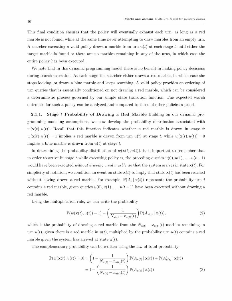
2.1.1. Stage t Probability of Drawing a Red Marble Building on our dynamic pro-

gramming modeling assumptions, we now develop the probability distribution associated with

w(x(t), u(t)). Recall that this function indicates whether a red marble is drawn in stage t:

w(x(t), u(t)) = 1 implies a red marble is drawn from urn u(t) at stage t, while w(x(t), u(t)) = 0

implies a blue marble is drawn from u(t) at stage t.

In determining the probability distribution of w(x(t), u(t)), it is important to remember that

in order to arrive in stage t while executing policy u, the preceding queries u(0), u(1), . . . , u(t− 1)

would have been executed without drawing a red marble, so that the system arrives in state x(t). For

simplicity of notation, we condition an event on state x(t) to imply that state x(t) has been reached

without having drawn a red marble. For example, P(Ai | x(t)) represents the probability urn i

contains a red marble, given queries u(0), u(1), . . . , u(t− 1) have been executed without drawing a

red marble.

Using the multiplication rule, we can write the probability

P(w(x(t), u(t)) = 1) =

(1

Nu(t)−xu(t)(t)

)P(Au(t) | x(t)), (2)

which is the probability of drawing a red marble from the Nu(t) − xu(t)(t) marbles remaining in

urn u(t), given there is a red marble in u(t), multiplied by the probability urn u(t) contains a red

marble given the system has arrived at state x(t).

The complementary probability can be written using the law of total probability:

P(w(x(t), u(t)) = 0) =

(1− 1

Nu(t)−xu(t)(t)

)P(Au(t) | x(t)) +P(Acu(t) | x(t))

= 1−(

1

Nu(t)−xu(t)(t)

)P(Au(t) | x(t)) (3)

Marks and Zaman: Multi-Urn Model for Network Search11

2.1.2. Stage t Urn Probabilities In this process, we have assumed a fully specified initial

probability model on the urns, i.e., for any subset U ⊆ V, the probability that a red marble is

present in all of the urns, ϕU , is known. This probability model can be thought of as a Bayesian

prior, a quantification of the searcher’s beliefs on where a red marble might be found.

However, these probabilities are not static. After drawing a marble from an urn, the probabilities

change as a result of the new information. If the marble drawn is red, then the probability that

a red marble existed in the queried urn becomes 1. Likewise, if the marble drawn is blue, then

the probability that a red marble can be found in the queried urn decreases as a function of the

number of marbles remaining in the urn and the current urn probability.

As long as a red marble is not found, the evolution of urn probabilities over the course of the

search is completely determined by the initial probability model and the search policy. We now

provide a general expression for updated urn probabilities at stage t.

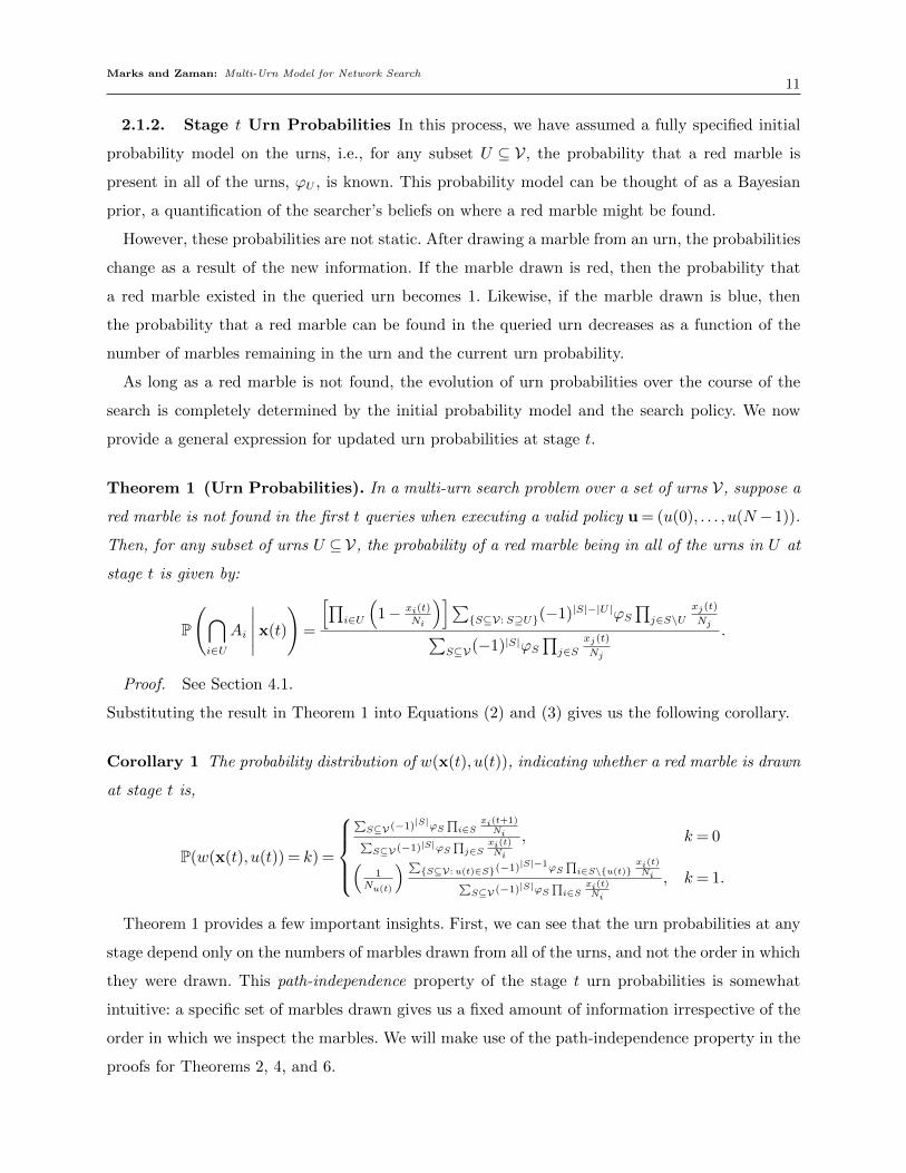
Theorem 1 (Urn Probabilities). In a multi-urn search problem over a set of urns V, suppose a

red marble is not found in the first t queries when executing a valid policy u = (u(0), . . . , u(N −1)).

Then, for any subset of urns U ⊆V, the probability of a red marble being in all of the urns in U at

stage t is given by:

P

(⋂i∈U

Ai

∣∣∣∣∣ x(t)

)=

[∏i∈U

(1− xi(t)

Ni

)]∑S⊆V: S⊇U(−1)|S|−|U |ϕS

∏j∈S\U

xj(t)

Nj∑S⊆V(−1)|S|ϕS

∏j∈S

xj(t)

Nj

.

Proof. See Section 4.1.

Substituting the result in Theorem 1 into Equations (2) and (3) gives us the following corollary.

Corollary 1 The probability distribution of w(x(t), u(t)), indicating whether a red marble is drawn

at stage t is,

P(w(x(t), u(t)) = k) =

∑S⊆V (−1)

|S|ϕS∏i∈S

xi(t+1)Ni∑

S⊆V (−1)|S|ϕS∏j∈S

xi(t)Ni

, k= 0(1

Nu(t)

) ∑S⊆V: u(t)∈S(−1)

|S|−1ϕS∏i∈S\u(t)

xi(t)Ni∑

S⊆V (−1)|S|ϕS∏i∈S

xi(t)Ni

, k= 1.

Theorem 1 provides a few important insights. First, we can see that the urn probabilities at any

stage depend only on the numbers of marbles drawn from all of the urns, and not the order in which

they were drawn. This path-independence property of the stage t urn probabilities is somewhat

intuitive: a specific set of marbles drawn gives us a fixed amount of information irrespective of the

order in which we inspect the marbles. We will make use of the path-independence property in the

proofs for Theorems 2, 4, and 6.

Marks and Zaman: Multi-Urn Model for Network Search12

Another observation is that the form of the probability expression is similar to the well-known

inclusion-exclusion formula for computing probabilities of unions of events. In fact, this probabil-

ity is an application of the principle of inclusion-exclusion applied in conjunction with Bayesian

updates. In Lemma 1, we explicitly define the events that are characterized by the inclusion-

exclusion formulas in Theorem 1.

2.2. Costs

In many network search applications, the cost of finding and examining a (random) neighbor of

a known vertex is primarily the time consumed in executing the query and reviewing the results

to determine whether the neighbor is the search target. Because we have no reason to believe this

time-cost would be different for different vertex-neighbor queries, we assume in our model that the

cost of drawing a marble is the same for all urns. The goal of the searcher is simply to minimize

the number of blue marbles drawn, or vertex-neighbor queries executed, before finding the search

target.

We therefore define the cost function at stage t,

g(t) =

1 w(x(t), u(t)) = 0

0 otherwise,

which applies a unit cost for every blue marble drawn. Because this quantity is stochastic, we set

as our objective the minimization of expected total cost. Letting random variable C =∑N

t=0 g(t),

we aim to find the optimal policy u to solve the following optimization problem:

minimizeu E [C] .

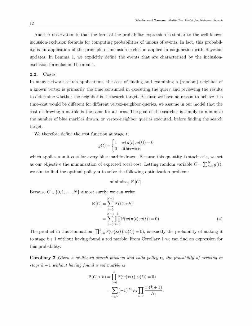
Because C ∈ 0,1, . . . ,N almost surely, we can write

E [C] =N−1∑k=0

P (C > k)

=N−1∑k=0

k∏t=0

P(w(x(t), u(t)) = 0). (4)

The product in this summation,∏k

t=0 P(w(x(t), u(t)) = 0), is exactly the probability of making it

to stage k+ 1 without having found a red marble. From Corollary 1 we can find an expression for

this probability.

Corollary 2 Given a multi-urn search problem and valid policy u, the probability of arriving in

stage k+ 1 without having found a red marble is

P(C > k) =k∏t=0

P(w(x(t), u(t)) = 0)

=∑S⊆V

(−1)|S|ϕS∏i∈S

xi(k+ 1)

Ni

.

Marks and Zaman: Multi-Urn Model for Network Search13

We can therefore rewrite the cost function,

E [C] =N−1∑t=0

∑S⊆V

(−1)|S|ϕS∏i∈S

xi(t+ 1)

Ni

. (5)

Substituting the probability from Corollary 2 into Corollary 1 reveals an interesting property of

the dynamics of this system:

P (w(x(t), u(t)) = 0) =P(C > t)

P(C > t− 1). (6)

3. Key Results

The cost function in equation (5) is nonlinear and nonconvex. Additionally, for a solution to be

feasible, the values for xi(t), i= 1, . . . , |V|, t= 0, . . . ,N must be constrained to correspond to stages

reached by a valid policy. Nonlinear, non-convex constrained optimization is difficult in general.

However, the structure of the cost function enables us to derive some useful results that characterize

the optimal solution in general, and provide necessary and sufficient conditions for optimality in

some specific cases.

3.1. Block Policy Optimality

We now provide our primary general result, in which we give a characterization of an optimal

search policy in the multi-urn search problem. We begin with a definition.

Definition 2 A block policy is a valid policy uB in which each urn is queried exhaustively

prior to querying another urn. A block policy can be specified as a sequence of urns uB =

(v1, v2, . . . , v|V|), vi ∈ V, implying

u(t) = vi,i−1∑j=1

Nj ≤ t <i∑

j=1

Nj.

This definition can be used to characterize the optimal policy, which we now formally state.

Theorem 2 (Block Policy Optimality). Given a multi-urn search problem in which the objec-

tive is to minimize the expected number of searches required to find a red marble, an optimal search

policy exists that is a block policy.

Proof. See Section 4.2.

This result says that an optimal policy for the multi-urn search problem can be characterized

by a sequence of urns. Once this is specified, one then simply searches each urn until it is out of

balls or a red ball is found. The surprising part of this result is that this block policy optimality

holds for arbitrary correlations in the a priori connection probabilities. For instance, there can be

Marks and Zaman: Multi-Urn Model for Network Search14

a negative correlation between two urns, where if the red ball is more likely to be in one urn, it is

less likely to be in another. In this case one may intuitively expect that after querying an urn many

times and not finding a red ball, at some point it might be advantageous to search another urn

which has a negative correlation with the queried urn. However, our result says that it is optimal

to continue querying the current urn until it is exhausted.

While Theorem 2 allows for optimal policies that are not block policies, constructing such a

case requires initial conditions that include probabilities that are zero. If ϕi,j > 0 for all pairs

i, j ⊂ V (as in the case of independent urns), then only block policies can be optimal policies.

This result follows from the proof of Theorem 2 (Section 4.2): observe that this condition implies

that function h(t) in equation (13) is strictly increasing in t, creating a contradiction in equation

(14).

We have shown that for mutli-urn search problems, a block policy is optimal, but we have not

yet specified what the block policy is. In general it can be difficult under arbitrary correlation

structures to find the optimal policy. However, under certain assumptions on the urn probability

model, explicit necessary and sufficient optimality conditions can be found. We examine these

conditions next.

3.2. Independent Urns

We now consider the special case in which the red marbles are assumed to be independently present

in each of the urns, so that the presence of a red marble in any urn (or group of urns) does not

affect the probability of a red marble being present in any other urn (or group of urns). This

probabilistic independence can be formalized mathematically.

Definition 3 An independent multi-urn search problem is a multi-urn search problem in which,

for any subset of urns, U ⊆V,

ϕU =∏i∈U

ϕi.

Intuitively, this independence property should be maintained throughout the search process for

any search policy, as we now show explicitly.

Theorem 3 (Independent Urn Probabilities). Given an independent multi-urn search prob-

lem, then for any policy u, at any stage t, the independence property is maintained so that

P

(⋂i∈U

Ai

∣∣∣∣∣ x(t)

)=∏i∈U

P(Ai|x(t)).

Proof. See Section 4.3

Marks and Zaman: Multi-Urn Model for Network Search15

It follows from the result in Theorem 3 that the probability of finding a red marble in stage t is

only a function of the initial conditions and number of times u(t) has been queried in the past.

The number of marbles that have previously been drawn from other urns i 6= u(t) do not affect

P(w(x(t), u(t)) = 1).

Because of the independence of the urn probabilities, we are able to obtain closed form expressions

for the probability of finding a red ball and the expected cost of a block policy, which are stated

in the following results.

Corollary 3 Given an independent multi-urn search problem, the probability distribution of

w(x(t), u(t)) at any stage t is

P(w(x(t), u(t)) = 0) =Nu(t)−xu(t)(t+ 1)ϕu(t)Nu(t)−xu(t)(t)ϕu(t)

.

Corollary 4 Given an independent multi-urn search problem and a block policy uB =

(v1, v2, . . . , v|V|), vi ∈ V, such that τ(i) =∑i−1

j=1Nvj is the first stage in which urn vi is queried.

Then,τ(i)+Ni−1∏t=τ(i)

P(w(x(t), u(t)) = 0) = (1−ϕvi),

the contribution of urn vi to the total expected cost is

τ(i)+Ni−1∑k=τ(i)

k∏t=0

P(w(x(t), u(t)) = 0) =

(Nvi −

(Nvi + 1)ϕvi

2

) i−1∏j=1

(1−ϕvj ),

and the total expected cost is

E[C] =

|V|∑i=1

(Ni−

(Ni + 1)ϕi2

) i−1∏j=1

(1−ϕj).

Independence implies that knowing the composition of marbles in urn i does not provide any

additional information on the compositions of marbles in any of the other urns. Drawing a marble

from urn u(t) in stage t still results in an update to this urn’s probability in stage t + 1, but

all other urn probabilities remain stationary in this state transition. This property enables us to

characterize the optimal policy in the case of independent urns.

Theorem 4 (Independent Urns Optimality) Given an independent multi-urn search problem,

a block policy

uB = (v1, v2, . . . , v|V|)

is optimal if and only if

Nvi

(2−ϕviϕvi

)≤Nvi+1

(2−ϕvi+1

ϕvi+1

), i= 1,2, . . . , |V|. (7)

Marks and Zaman: Multi-Urn Model for Network Search16

Proof. See Section 4.4.

We note that this policy is not greedy, i.e., it does not maximize the probability of finding the

red marble at each stage. Rather, the optimality condition in equation (7) balances the probability

of immediately drawing a red marble with the probability of finding a red marble in successive

draws from the same urn.

To gain intuition, consider a two-urn example in which each urn has the same probability of

containing a red marble (ϕ1 = ϕ2), but urn 1 has fewer marbles (N1 <N2). In this case the opti-

mality condition in equation (7) would have us initially draw marbles from urn 1, which has the

same probability of giving us the red marble as urn 2 but requires fewer draws.

Alternatively, consider the case in which the two urns have the same number of marbles but

ϕ1 <ϕ2. In this case, the optimal policy according to equation (7) would have us draw from urn 2

first, which is more likely than urn 1 to give us a red marble in the same number of draws.

In order to more clearly distinguish between a greedy policy and an optimal one, we provide one

more example. Consider the following independent multi-urn search problem with two urns. Urn

1 contains N1 = 1 marble and has probability ϕ1 = 916

of containing a red marble. Urn 2 contains

N2 = 2 marbles and has probability ϕ2 = 1 of containing a red marble. This problem admits two

block policies: uB = (2,1) and uB = (1,2).

Policy uB is a greedy policy; urn 1, which has the highest immediate probability of producing a

red marble ( 916

), is queried before urn 2. The expected number of blue marbles drawn using policy

uB is

E[C] =7

16+

(7

16

)(1

2

)=

21

32.

Alternatively, if we follow policy uB and draw from urn 2 first, then expected cost is

E[C] =1

2,

which is optimal. By accepting a slightly lower probability in the first draw, this policy guarantees

that the red marble is found in at most two draws. The optimality condition in Theorem 4, equation

(7) provides the best balance between the immediate and long-term benefits of each query.

3.3. One Marble

We now turn our attention to another special case of the multi-urn search problem in which we

limit the total number of red marbles among all of the urns to a single marble. In our network

search scenario, this constraint would follow from assuming that the target user is connected to at

most one of the known accounts on Mary’s list. This might not be a valid assumption for Mary to

make, but it might apply to other search scenarios both in and out of the network context.

Marks and Zaman: Multi-Urn Model for Network Search17

For example, suppose law enforcement investigators have evidence that a suspect made a single

phone call from an unknown phone number during a certain period. Having obtained phone records

from all likely recipients, they must efficiently search for the phone call of interest within the records

of these likely recipients.

For a non-network example, suppose a hotel custodian, after servicing all of the hotel rooms,

realizes he left his car keys in one of the rooms. The hotel might consist of several wings, each with

different numbers of rooms, and the custodian might feel the loss was more probable in certain

wings. The custodian wants to search the rooms efficiently for his keys, in order to find them before

new customers begin to arrive.

This one-marble constraint imposes the strongest negative correlations between the urns: if the

red marble is in urn i then it cannot be in j, i.e.,

P (Aj|Ai) = 0, i 6= j.

Another way to characterize this constraint is to state that the events A1,A2, . . . ,A|V| are disjoint.

We now formalize this notion in a definition.

Definition 4 A single marble multi-urn search problem is a multi-urn search problem for which

ϕU = 0 ∀ U ⊆V such that |U |> 1.

We now analyze of the single marble search problem. First we observe that∑i∈V

ϕi ≤ 1.

We allow for the possibility that this sum is strictly less than one, implying there is a chance

that none of the urns contain the red marble. If the sum is equal to one, then the assumption is

that exactly one of the urns contains one red marble. Theorem 5 specifies the single marble urn

probabilities for an arbitrary state x(t).

Theorem 5 (Single Marble Urn Probabilities). Given a single marble multi-urn search prob-

lem and a search policy u. Then, the probability that a red marble is in urn i given state x(t), and

given no red marble has been found in the first t queries, is

P(Ai | x(t)) =

(1− xi(t)

Ni

)ϕi

1−∑

j∈Vxj(t)ϕjNj

.

The probability that the red marble is in all of the urns in any subset U ⊂V, where |U |> 1 is

P

(⋂i∈U

Ai

∣∣∣∣∣ x(t)

)= 0.

Marks and Zaman: Multi-Urn Model for Network Search18

Proof. This result follows immediately from the definition of a single marble multi-urn search

problem and Theorem 1.

Because the red ball can only be in one urn, all joint probabilities are zero. This greatly simplifies

our analysis and allows us to obtain closed form expressions for the probability of finding a red

ball and the expected cost of a block policy, which are stated in the following results.

Corollary 5 Given a single marble multi-urn search problem and a valid search policy u, the

probability distribution of w(x(t), u(t)), conditioned on not having found a red marble in a previous

stages, is

P(w(x(t), u(t)) = k) =

1−∑j∈V

(xj(t+1)ϕj

Nj

)1−∑j∈V

(xj(t)ϕjNj

) , k= 0

1Nu(t)

(ϕu(t)

1−∑j∈V

(xj(t)ϕjNj

)), k= 1.

Corollary 6 Given a single marble multi-urn problem and a block policy uB =

(v1, v2, . . . , v|V|), vi ∈ V, such that τ(i) =∑i−1

j=1Nvj is the first stage in which urn vi is queried.

Then, the probability of not finding the red marble before reaching stage τ(i) is

τ(i)∏t=0

P(w(x(t), u(t)) = 0) = 1−i−1∑j=1

ϕvj ,

the contribution of urn vi to the total expected cost is

τ(i)+Ni−1∑k=τ(i)

k∏t=0

P(w(x(t), u(t)) = 0) =

(Ni−

(Ni + 1)ϕi2

−Ni

i−1∑j=1

ϕj

),

and the total expected cost is

E[C] =

|V|∑i=1

(Nvi −

(Nvi + 1)ϕvi

2

)−|V|−1∑i=1

|V|∑j=i+1

Nvjϕvi .

Theorem 6 characterizes the optimal solution in the single marble case.

Theorem 6 (Single Marble Optimality). Given a single marble multi-urn search problem, a

block policy

uB = (v1, v2, . . . , v|V|)

is an optimal policy if and only if

ϕvi

Nvi≥ ϕvi+1

Nvi+1

, i= 1,2, . . . , |V|. (8)

Proof. See Section 4.5.

Marks and Zaman: Multi-Urn Model for Network Search19

The optimality condition given in equation (8) leads to a greedy policy in which, at each stage,

the marble that is drawn is the one that is most likely to be red. At stage t= 0 this is certainly true,

as the probability of drawing a red marble from any urn i in the first draw is ϕi/Ni, which is exactly

what the optimality condition optimizes. In the next section we show that that this condition is

maintained through state transitions in an optimal policy. If drawing a marble from urn i has the

highest probability of producing a red marble in stage t, then (assuming the urn has at least one

marble remaining) drawing another marble from the same urn maximizes the probability of finding

a red marble in stage t+ 1.

3.4. Monotonicity Properties

We now provide a few monotonicity properties that give additional insight into the dynamics of

multi-urn search problems, as well as block policy optimality.

Theorem 7 (Monotonicity). Given a multi-urn search problem and a search policy u, the fol-

lowing inequalities hold:

1. For any subset of urns U ⊆V such that u(t)∈U ,

P

(⋂i∈U

Ai

∣∣∣∣∣ x(t)

)≥ P

(⋂i∈U

Ai

∣∣∣∣∣ x(t+ 1)

),

with equality holding only in cases in which P(Au(t) | x(t)

)= 1 or P

(⋂i∈U Ai | x(t)

)= 0.

2. For any stage t for which urn u(t) has more than one marble remaining, i.e., Nu(t)−xu(t)(t)>

1,

P(w(x(t), u(t)) = 1)≤ P(w(x(t+ 1), u(t)) = 1),

with equality holding only when P(w(x(t), u(t)) = 1) = 0.

Proof. See Section 4.6.

These monotonicity properties provide intuition into why optimal block policies exist. Suppose

at stage t a blue marble is drawn from urn u(t). At stage t+1, the probability of urn u(t) containing

a red marble has decreased as a result of this new information. However, the probability that the

next marble drawn from urn u(t) is red has increased from the previous stage. If drawing from urn

u(t) in stage t had a high probability of returning a red marble, drawing another marble from u(t)

in stage t+ 1 has an even higher probability of producing a red marble.

In the case of independent urns, this property provides justification for using a block policy.

Suppose urn u(t) has multiple marbles in it and is optimal at stage t, and a blue marble is drawn

from this urn. At stage t+ 1 the probability of drawing a red marble from urn u(t) has increased,

while all other urn and marble probabilities have remained unchanged from the previous stage t.

It follows that it would continue to be optimal to draw from urn u(t).

Marks and Zaman: Multi-Urn Model for Network Search20

If we allow for correlations among the urns, however, drawing a blue marble from urn u(t) might

also increase the probability of drawing a red marble from other urns in the following stage. In the

single marble multi-urn search problem, drawing a blue marble from urn u(t) in stage t increases

the probability of finding a red marble in each of the other urns in stage t+ 1. We now provide our

final theoretical result, which states that the rate of probability growth in a queried urn is always

at least as large as the rate of probability growth in any other urn.

Theorem 8 (Marble Probability Bound). Given a multi-urn search problem and a search

policy u, the following inequality holds:

P (w(x(t+ 1), u(t)) = 1)

P (w(x(t), u(t)) = 1)≥ P (w(x(t+ 1), i) = 1)

P (w(x(t), i) = 1).

Proof. See Section 4.7.

Theorem 8 provides much intuition about why optimal block policies always exist in multi-urn

search problems. It also shows that a purely greedy strategy, in which the probability of immediately

drawing a red marble is maximized at each stage, will always produce a (possibly suboptimal) block

policy. Finally, it provides some insight into why the optimality conditions for the single marble

multi-urn search problem given in equation (8) result in a greedy policy. Equation (8) specifies that

the first marble drawn is the one that maximizes the probability of immediately finding the target.

It follows from Theorem 8 that subsequent draws from the same urn will continue to maximize

this probability.

3.5. Urn Correlation Dynamics

In the preceding section we examined how urn probabilities and the probability of drawing a red

marble from each urn evolved as a function of the state of the system. In this section we show by

example how, in general, the correlations among the urns can evolve in ways that we find to be

counterintuitive.

We say that two urns i and j are positively correlated at stage t if they have positive covariance,

i.e.,

P (Ai ∩Aj | x(t))> P (Ai | x(t))P (Aj | x(t)) .

Likewise, urns i and j are negatively correlated if their covariance is negative,

P (Ai ∩Aj | x(t))< P (Ai | x(t))P (Aj | x(t)) .

In Theorem 3 we showed the somewhat intuitive result that independence among the urn proba-

bilities is preserved through state transitions. In general, correlations can change through Bayesian

updates each time a blue marble is drawn. These changes can include changes in sign.

Marks and Zaman: Multi-Urn Model for Network Search21

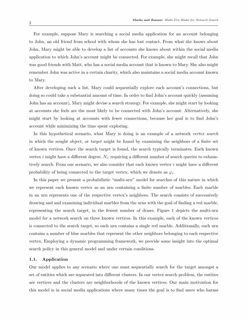
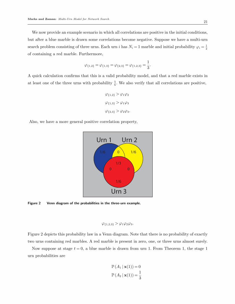
We now provide an example scenario in which all correlations are positive in the initial conditions,

but after a blue marble is drawn some correlations become negative. Suppose we have a multi-urn

search problem consisting of three urns. Each urn i has Ni = 1 marble and initial probability ϕi = 12

of containing a red marble. Furthermore,

ϕ1,2 =ϕ1,3 =ϕ2,3 =ϕ1,2,3 =1

3.

A quick calculation confirms that this is a valid probability model, and that a red marble exists in

at least one of the three urns with probability 56. We also verify that all correlations are positive,

ϕ1,2 >ϕ1ϕ2

ϕ1,3 >ϕ1ϕ3

ϕ2,3 >ϕ2ϕ3.

Also, we have a more general positive correlation property,

Urn 1

1/61/6

1/6

1/30 0

0

Urn 2

Urn 3

Figure 2 Venn diagram of the probabilities in the three-urn example.

ϕ1,2,3 >ϕ1ϕ2ϕ3.

Figure 2 depicts this probability law in a Venn diagram. Note that there is no probability of exactly

two urns containing red marbles. A red marble is present in zero, one, or three urns almost surely.

Now suppose at stage t= 0, a blue marble is drawn from urn 1. From Theorem 1, the stage 1

urn probabilities are

P (A1 | x(1)) = 0

P (A2 | x(1)) =1

3

Marks and Zaman: Multi-Urn Model for Network Search22

P (A3 | x(1)) =1

3

P (A1 ∩A2 | x(1)) = 0

P (A1 ∩A3 | x(1)) = 0

P (A2 ∩A3 | x(1)) = 0

P (A1 ∩A2 ∩A3 | x(1)) = 0.

By eliminating the possibility that each urn contained a red marble, the only outcomes that have

positive probability in stage 1 are single-marble outcomes. The correlation between urns 2 and 3,

which was positive in the initial conditions, has become negative in stage 1:

P (A2 ∩A3 | x(1)) = 0<1

9= P (A2 | x(1))P (A3 | x(1)) .

One could similarly produce examples in which correlations that were originally negative become

positive after drawing blue marbles. In the single-marble and independent urn cases, for which we

provided characterizations of the optimal policies in the preceding sections, correlations among the

urns exhibited some stationarity with respect to stage. In general, the nature of correlations among

the urns can change substantially as blue marbles are drawn and probabilities are updated. This

characteristic presents a challenge to finding characterizations of the optimal policy in general.

4. Proofs of Theorems

In this section we provide the technical proof for each theorem.

4.1. Theorem 1

Proof of Theorem 1 Substituting the initial condition, x(0) = 0, into the result returns the

prior

P

(⋂i∈U

Ai

∣∣∣∣∣ x(0)

)=ϕU := P

(⋂i∈U

Ai

).

The proof proceeds by induction. First note that in order to reach state x(t+ 1) from stage

t, a blue marble must have been drawn from urn u(t) from state x(t). We use the law of total

probability to decompose this event and form a recursion:

P

(⋂i∈U

Ai

∣∣∣∣∣ x(t+ 1)

)=

P((⋂

i∈U Ai)∩w(x(t), u(t)) = 0|x(t)

)P(w(x(t), u(t)) = 0)

=

(1− 1

Nu(t)−xu(t)(t)

)P(⋂

i∈U∪u(t)Ai

∣∣∣ x(t))

+P(Acu(t) ∩(⋂

i∈U Ai)|x(t))

1−(

1Nu(t)−xu(t)(t)

)P(Au(t)|x(t))

=P(⋂

i∈U Ai∣∣ x(t)

)−(

1Nu(t)−xu(t)(t)

)P(⋂

i∈U∪u(t)Ai

∣∣∣ x(t))

1−(

1Nu(t)−xu(t)(t)

)P(Au(t)|x(t))

(9)

Marks and Zaman: Multi-Urn Model for Network Search23

The result in Theorem 1 forms our induction hypothesis. We use this result to form the three

probabilities in the recursion given in equation (9).

P

(⋂i∈U

Ai

∣∣∣∣∣ x(t)

)=

[∏i∈U

(1− xi(t)

Ni

)]∑S⊆V: S⊇U(−1)|S|−|U |ϕS

∏j∈S\U

xj(t)

Nj∑S⊆V(−1)|S|ϕS

∏j∈S

xj(t)

Nj

P(Au(t)|x(t)

)=

(1− xu(t)(t)

Nu(t)

)∑S⊆V: u(t)∈S(−1)|S|−1ϕS

∏j∈S\u(t)

xj(t)

Nj∑S⊆V(−1)|S|ϕS

∏j∈S

xj(t)

Nj

P

⋂i∈U∪u(t)

Ai

∣∣∣∣∣∣ x(t)

=

[∏i∈U

(1−xi(t)Ni

)]∑S⊆V: S⊇U(−1)

|S|−|U|ϕS∏j∈S\U

xj(t)

Nj∑S⊆V (−1)|S|ϕS

∏j∈S

xj(t)

Nj

u(t)∈U[∏

i∈(U∪u(t))(1−xi(t)Ni

)]∑S⊆V: S⊇(U∪u(t))(−1)

|S|−|U|−1ϕS∏j∈S\(U∪u(t))

xj(t)

Nj∑S⊆V (−1)|S|ϕS

∏j∈S

xj(t)

Nj

u(t) /∈U.

As we see from these probabilities, we have two cases to consider:

1. u(t)∈U .

2. u(t) /∈U .

We now look at each of these cases individually.

Case 1: u(t)∈U . We begin by substituting the probabilities formed using the induction hypoth-

esis into the recursion in equation (9).

P

(⋂i∈U

Ai

∣∣∣∣∣ x(t+ 1)

)=

P(⋂

i∈U Ai∣∣ x(t)

)−(

1Nu(t)−xu(t)(t)

)P(⋂

i∈U∪u(t)Ai

∣∣∣ x(t))

1−(

1Nu(t)−xu(t)(t)

)P(Au(t)|x(t))

=

(1− 1

Nu(t)−xu(t)(t)

) [∏i∈U

(1−xi(t)Ni

)]∑S⊆V: S⊇U(−1)

|S|−|U|ϕS∏j∈S\U

xj(t)

Nj∑S⊆V (−1)|S|ϕS

∏j∈S

xj(t)

Nj

1−(

1Nu(t)−xu(t)(t)

)((1−xu(t)(t)Nu(t)

)∑S⊆V: u(t)∈S(−1)|S|−1ϕS

∏j∈S\u(t)

xj(t)

Nj∑S⊆V (−1)|S|ϕS

∏j∈S

xj(t)

Nj

)

=

(Nu(t)−xu(t)(t)−1Nu(t)−xu(t)(t)

) [(Nu(t)−xu(t)(t)Nu(t)

)∏i∈U\u(t)

(1−xi(t)Ni

)]∑S⊆V: S⊇U(−1)

|S|−|U|ϕS∏j∈S\U

xj(t)

Nj∑S⊆V (−1)|S|ϕS

∏j∈S

xj(t)

Nj

1−(

1Nu(t)

)(∑S⊆V: u(t)∈S(−1)|S|−1ϕS

∏j∈S\u(t)

xj(t)

Nj∑S⊆V (−1)|S|ϕS

∏j∈S

xj(t)

Nj

)We proceed by separating the summations into terms corresponding to sets containing u(t) and

those that do not contain u(t). We can then factor out the terms corresponding to urn u(t) and

make the following substitutions:

xi(t) =

xi(t+ 1) i 6= u(t)

xi(t+ 1)− 1 i= u(t).

Marks and Zaman: Multi-Urn Model for Network Search24

Continuing the simplification from above,

=

(Nu(t)−xu(t)(t+1)

Nu(t)

)[∏i∈U\u(t)

(1− xi(t+1)

Ni

)]∑S⊆V: S⊇U(−1)|S|−|U |ϕS

∏j∈S\U

xj(t+1)

Nj∑S⊆V(−1)|S|ϕS

∏j∈S

xj(t)

Nj−(

1Nu(t)

)(∑S⊆V: u(t)∈S(−1)|S|−1ϕS

∏j∈S\u(t)

xj(t)

Nj

)=

[∏i∈U

(1− xi(t+1)

Ni

)]∑S⊆V: S⊇U(−1)|S|−|U |ϕS

∏j∈S\U

xj(t+1)

Nj∑S⊆V\u(t)(−1)|S|ϕS

∏j∈S

xj(t)

Nj+(xu(t)(t)

Nu(t)+ 1

Nu(t)

)(∑S⊆V: u(t)∈S(−1)|S|ϕS

∏j∈S\u(t)

xj(t)

Nj

)=

[∏i∈U

(1− xi(t+1)

Ni

)]∑S⊆V: S⊇U(−1)|S|−|U |ϕS

∏j∈S\U

xj(t+1)

Nj∑S⊆V\u(t)(−1)|S|ϕS

∏j∈S

xj(t+1)

Nj+∑S⊆V: u(t)∈S(−1)|S|ϕS

∏j∈S

xj(t+1)

Nj

=

[∏i∈U

(1− xi(t+1)

Ni

)]∑S⊆V: S⊇U(−1)|S|−|U |ϕS

∏j∈S\U

xj(t+1)

Nj∑S⊆V(−1)|S|ϕS

∏j∈S

xj(t+1)

Nj

.

Observe that this is the desired result for stage t+ 1. We now provide the induction step for the

case in which u(t) /∈U .

Case 2: u(t) /∈U follows a similar set of steps. We begin by substituting the probabilities formed

using the induction hypothesis into the recursion in equation (9).

P(⋂

i∈U Ai∣∣ x(t)

)−(

1Nu(t)−xu(t)(t)

)P(⋂

i∈U∪u(t)Ai

∣∣∣ x(t))

1−(

1Nu(t)−xu(t)(t)

)P(Au(t)|x(t))

=

[(∏i∈U

(1− xi(t)

Ni

))∑S⊆V: S⊇U(−1)|S|−|U |ϕS

∏j∈S\U

xj(t)

Nj∑S⊆V(−1)|S|ϕS

∏j∈S

xj(t)

Nj

−

(1

Nu(t)−xu(t)(t)

)(∏i∈U∪u(t)

(1− xi(t)

Ni

))∑S⊆V: S⊇U∪u(t)(−1)|S|−|U |−1ϕS

∏j∈S\(U∪u(t))

xj(t)

Nj∑S⊆V(−1)|S|ϕS

∏j∈S

xj(t)

Nj

]

×

[1−

(1

Nu(t)−xu(t)(t)

)(

1− xu(t)(t)

Nu(t)

)∑S⊆V: u(t)∈S(−1)|S|−1ϕS

∏j∈S\u(t)

xj(t)

Nj∑S⊆V(−1)|S|ϕS

∏j∈S

xj(t)

Nj

]−1The denominators in the above expression reduce in exactly the same way as in the previous

case in which u(t) ∈ U . In fact, the denominators in the induction hypothesis and in equation

(9) do not depend on whether u(t) ∈ U . Because we have already shown the steps for reducing

this denominator to the desired form, we omit these steps and only show the induction on the

numerators for this case:

[(∏i∈U

(1− xi(t)

Ni

)) ∑S⊆V: S⊇U

(−1)|S|−|U |ϕS∏

j∈S\U

xj(t)

Nj

−(

1

Nu(t)−xu(t)(t)

) ∏i∈U∪u(t)

(1− xi(t)

Ni

) ∑S⊆V: S⊇U∪u(t)

(−1)|S|−|U |−1ϕS∏

j∈S\(U∪u(t))

xj(t)

Nj

]

Marks and Zaman: Multi-Urn Model for Network Search25

=

(∏i∈U

(1− xi(t)

Ni

))[ ∑S⊆V: S⊇U

(−1)|S|−|U |ϕS∏

j∈S\U

xj(t)

Nj

+

(1

Nu(t)−xu(t)(t)

)(Nu(t)−xu(t)(t)

Nu(t)

) ∑S⊆V: S⊇U∪u(t)

(−1)|S|−|U |ϕS∏

j∈S\(U∪u(t))

xj(t)

Nj

]

=

(∏i∈U

(1− xi(t)

Ni

))[ ∑S⊆V\u(t): S⊇U

(−1)|S|−|U |ϕS∏

j∈S\U

xj(t)

Nj

+

(xu(t)(t)

Nu(t)

+1

Nu(t)

) ∑S⊆V: S⊇U∪u(t)

(−1)|S|−|U |ϕS∏

j∈S\(U∪u(t))

xj(t)

Nj

]

We again make the substitution:

xi(t) =

xi(t+ 1) i 6= u(t)

xi(t+ 1)− 1 i= u(t),

and continue from above:

=

(∏i∈U

(1− xi(t+ 1)

Ni

))[ ∑S⊆V\u(t): S⊇U

(−1)|S|−|U |ϕS∏

j∈S\U

xj(t+ 1)

Nj

+

(xu(t)(t+ 1)

Nu(t)

) ∑S⊆V: S⊇U∪u(t)

(−1)|S|−|U |ϕS∏

j∈S\(U∪u(t))

xj(t+ 1)

Nj

]

=

(∏i∈U

(1− xi(t+ 1)

Ni

)) ∑S⊆V: S⊇U

(−1)|S|−|U |ϕS∏

j∈S\U

xj(t+ 1)

Nj

.

This final expression is the numerator in Theorem 1 for the stage t+ 1 urn probabilities.

4.2. Theorem 2

Before we provide a proof for Theorem 2, we state and prove the following Lemma.

Lemma 1 Given a multi-urn search problem on a set of urns V, suppose a policy u is executed

to stage t irrespective of whether a red marble is found at any stage. Let Bi be the event that a

red marble has been drawn from urn i ∈ V in this experiment. Then, for any subset U ⊆ V, the

probability of having drawn a red marble from each of the urns in U and none of the other urns is

P

(⋂i∈U

Bi

)∩

⋂j∈V\U

Bcj

=∑

S:S⊆V,S⊇U

(−1)|S|−|U |ϕS∏i∈S

xi(t)

Ni

≥ 0.

Proof of Lemma 1. This result is comes from the principle of inclusion-exclusion, and fol-

lows from Equation 1. From basic set operations and DeMorgan’s Law, we can write(⋂i∈U

Bi

)=

(⋂i∈U

Bi

)∩

⋂j∈V\U

Bcj

∪(⋂

i∈U

Bi

)∩

⋃j∈V\U

Bj

,

Marks and Zaman: Multi-Urn Model for Network Search26

which is a union of disjoint sets. Therefore,

P

(⋂i∈U

Bi

)∩

⋂j∈V\U

Bcj

= P

(⋂i∈U

Bi

)−P

(⋂i∈U

Bi

)∩

⋃j∈V\U

Bj

. (10)

The probability a red marble is drawn from all of the urns in U in this experiment can be found

using the multiplication rule:

P

(⋂i∈U

Bi

)=ϕU

∏i∈U

xi(t)

Ni

. (11)

Recall that ϕU is the probability of all of the urns in set U containing a red marble, and xi(t)

Niis

simply the fraction of marbles removed from urn i at stage t. The product in this expression implies

conditional independence: given all of the urns in U contain a red marble, the probability that a

red marble is drawn from each of them by stage t is the product of the individual probabilities.

This conditional independence follows implicitly from our search assumptions. The order of marble

draws from each urn is random, and does not depend on the order of marble draws from any other

urn.

We now examine P((⋂

i∈U Bi)∩(⋃

j∈V\U Bj

)). We first note that(⋂

i∈U

Bi

)∩

⋃j∈V\U

Bj

=⋃

j∈V\U

((⋂i∈U

Bi

)∩Bj

).

Using the principle of inclusion exclusion, we can find the probability of this union,

P

⋃j∈V\U

((⋂i∈U

Bi

)∩Bj

)=∑j∈V\U

P

((⋂i∈U

Bi

)∩Bj

)

−∑j∈V\U

∑k∈V\(U∪j)

P

((⋂i∈U

Bi

)∩Bj ∩Bk

)· · ·+ (−1)|V|−|U |+1P

(⋂i∈V

Bi

). (12)

Substituting expressions 11 and 12 into equation 10 reduces to the desired result. The principle of

inclusion-exclusion and the axioms of probability ensure that this quantity is nonnegative.

We now provide the proof of Theorem 2.

Proof of Theorem 2. Suppose we are given a multi-urn search problem on a set of urns

V, with each urn i ∈ V containing Ni marbles and initial target probabilities ϕU for all U ⊆ V.

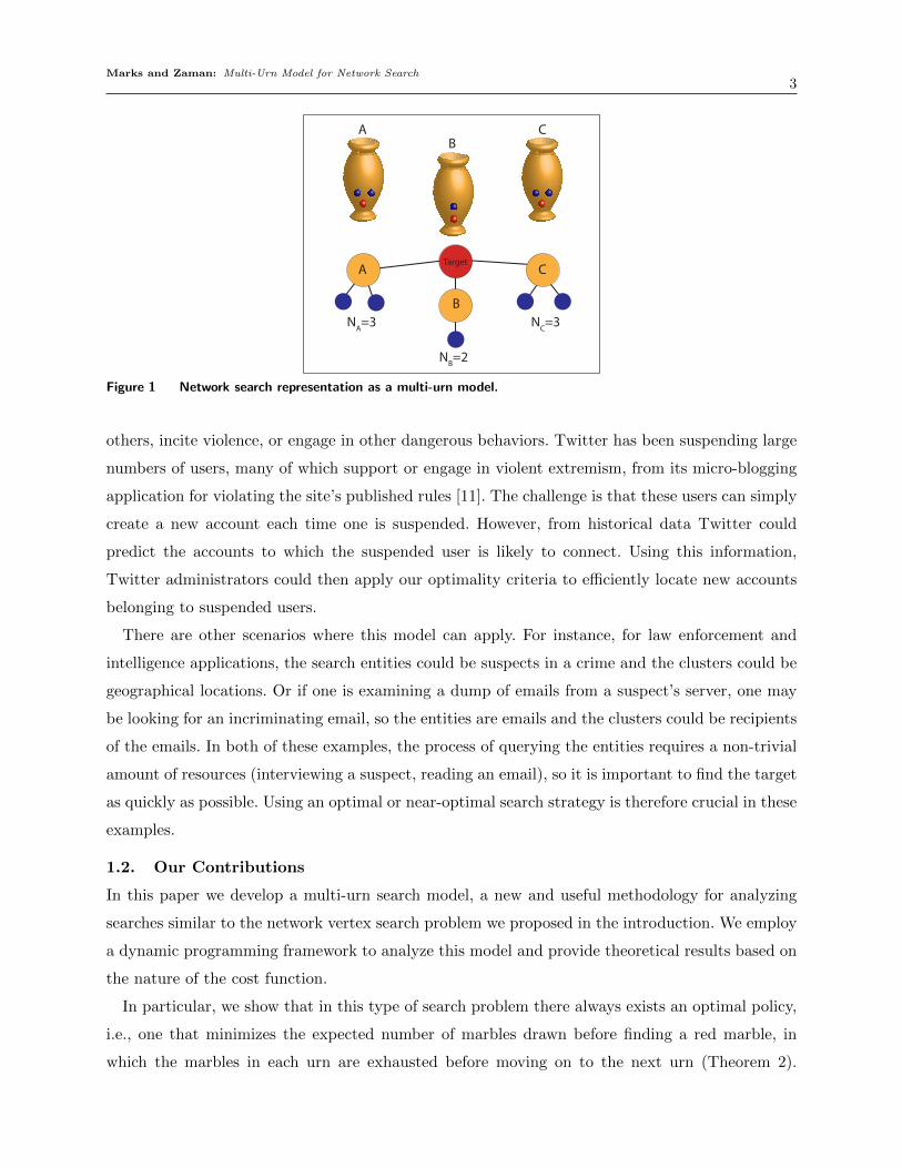
Suppose also that valid policy u = (u(0), . . . , u(N − 1)) is optimal, where u is not a block policy.

This implies that we can find a stage τ where

u(τ) = i

u(τ + 1), u(τ + 2), . . . , u(τ + δ− 1) 6= i

u(τ + δ) = i,

Marks and Zaman: Multi-Urn Model for Network Search27

for some urn i∈ V, where δ > 1.

h i j k i l

h i i k l

ττ−1 τ+1 τ+δ τ+δ+1...u(t)

t

^

ττ−1 τ+1 τ+δ−1 τ+δ τ+δ+1...u(t)

t

h j l

ττ−1 τ+δ−1 τ+δ τ+δ+1...u(t)

t

i i~

j

τ+2

k

τ+δ−2

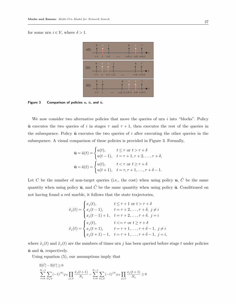
Figure 3 Comparison of policies u, u, and u.

We now consider two alternative policies that move the queries of urn i into “blocks”. Policy

u executes the two queries of i in stages τ and τ + 1, then executes the rest of the queries in

the subsequence. Policy u executes the two queries of i after executing the other queries in the

subsequence. A visual comparison of these policies is provided in Figure 3. Formally,

u = u(t) =

u(t), t≤ τ or t > τ + δ

u(t− 1), t= τ + 1, τ + 2, . . . , τ + δ,

u = u(t) =

u(t), t < τ or t≥ τ + δ

u(t+ 1), t= τ, τ + 1, . . . , τ + δ− 1.

Let C be the number of non-target queries (i.e., the cost) when using policy u, C be the same

quantity when using policy u, and C be the same quantity when using policy u. Conditioned on

not having found a red marble, it follows that the state trajectories,

xj(t) =

xj(t), t≤ τ + 1 or t > τ + δ

xj(t− 1), t= τ + 2, . . . , τ + δ, j 6= i

xj(t− 1) + 1, t= τ + 2, . . . , τ + δ, j = i

xj(t) =

xj(t), t <= τ or t≥ τ + δ

xj(t+ 1), t= τ + 1, . . . , τ + δ− 1, j 6= i

xj(t+ 1)− 1, t= τ + 1, . . . , τ + δ− 1, j = i,

where xj(t) and xj(t) are the numbers of times urn j has been queried before stage t under policies

u and u, respectively.

Using equation (5), our assumptions imply that

E[C]−E[C] ≥ 0

N−1∑t=0

∑S⊆V

(−1)|S|ϕS∏j∈S

xj(t+ 1)

Nj−N−1∑t=0

∑S⊆V

(−1)|S|ϕS∏j∈S

xj(t+ 1)

Nj≥ 0

Marks and Zaman: Multi-Urn Model for Network Search28

∑S⊆V\i

(τ+δ∑t=τ+2

(−1)|S|ϕS∏j∈S

xj(t)

Nj−

τ+δ∑t=τ+2

(−1)|S|ϕS∏j∈S

xj(t)

Nj

)

+∑

S⊆V:i∈S

(τ+δ∑t=τ+2

(−1)|S|ϕS∏j∈S

xj(t)

Nj−

τ+δ∑t=τ+2

(−1)|S|ϕS∏j∈S

xj(t)

Nj

)≥ 0

∑S⊆V\i

(τ+δ−1∑t=τ+1

(−1)|S|ϕS∏j∈S

xj(t)

Nj−

τ+δ∑t=τ+2

(−1)|S|ϕS∏j∈S

xj(t)

Nj

)

+∑

S⊆V:i∈S

τ+δ−1∑t=τ+1

(−1)|S|ϕS

(xi(t) + 1

Ni

) ∏j∈S\i

xj(t)

Nj−

τ+δ∑t=τ+2

(−1)|S|ϕS

(xi(t)

Ni

) ∏j∈S\i

xj(t)

Nj

≥ 0

∑S⊆V\i

((−1)|S|ϕS

∏j∈S

xj(τ + 1)

Nj− (−1)|S|ϕS

∏j∈S

xj(τ + δ)

Nj

)

+∑

S⊆V:i∈S

(xi(τ + δ)

Ni

)(−1)|S|ϕS∏

j∈S\i

xj(τ + 1)

Nj− (−1)|S|ϕS

∏j∈S\i

xj(τ + δ)

Nj

+

1

Ni

∑S⊆V:i∈S

τ+δ−1∑t=τ+1

(−1)|S|ϕS∏

j∈S\i

xj(t)

Nj≥ 0

∑S⊆V\i

((−1)|S|ϕS

∏j∈S

xj(τ + δ)

Nj− (−1)|S|ϕS

∏j∈S

xj(τ + 1)

Nj

)

+∑

S⊆V:i∈S

(xi(τ + δ)

Ni

)(−1)|S|ϕS∏

j∈S\i

xj(τ + δ)

Nj− (−1)|S|ϕS

∏j∈S\i

xj(τ + 1)

Nj

− 1

Ni

∑S⊆V:i∈S

τ+δ−1∑t=τ+2

(−1)|S|ϕS∏

j∈S\i

xj(t)

Nj≤ 1

Ni

∑S⊆V:i∈S

(−1)|S|ϕS∏

j∈S\i

xj(τ + 1)

Nj.

Optimality of u likewise implies

E[C]−E[C] ≥ 0

N−1∑t=0

∑S⊆V

(−1)|S|ϕS∏j∈S

xj(t+ 1)

Nj−N−1∑t=0

∑S⊆V

(−1)|S|ϕS∏j∈S

xj(t+ 1)

Nj≥ 0

∑S⊆V

(τ+δ−1∑t=τ+1

(−1)|S|ϕS∏j∈S

xj(t)

Nj−τ+δ−1∑t=τ+1

(−1)|S|ϕS∏j∈S

xj(t)

Nj

)≥ 0

∑S⊆V\i

(τ+δ−1∑t=τ+1

(−1)|S|ϕS∏j∈S

xj(t)

Nj−τ+δ−1∑t=τ+1

(−1)|S|ϕS∏j∈S

xj(t)

Nj

)

+∑

S⊆V:i∈S

(τ+δ−1∑t=τ+1

(−1)|S|ϕS∏j∈S

xj(t)

Nj−τ+δ−1∑t=τ+1

(−1)|S|ϕS∏j∈S

xj(t)

Nj

)≥ 0

∑S⊆V\i

(τ+δ∑t=τ+2

(−1)|S|ϕS∏j∈S

xj(t)

Nj−τ+δ−1∑t=τ+1

(−1)|S|ϕS∏j∈S

xj(t)

Nj

)

+∑

S⊆V:i∈S

τ+δ∑t=τ+2

(−1)|S|ϕS

(xi(t)− 1

Ni

) ∏j∈S\i

xj(t)

Nj−τ+δ−1∑t=τ+1

(−1)|S|ϕS

(xi(t)

Ni

) ∏j∈S\i

xj(t)

Nj

≥ 0

∑S⊆V\i

((−1)|S|ϕS

∏j∈S

xj(τ + δ)

Nj− (−1)|S|ϕS

∏j∈S

xj(τ + 1)

Nj

)

+∑

S⊆V:i∈S

(−1)|S|ϕS

(xi(τ + δ)− 1

Ni

) ∏j∈S\i

xj(τ + δ)

Nj− (−1)|S|ϕS

(xi(τ + 1)

Ni

) ∏j∈S\i

xj(τ + 1)

Nj

Marks and Zaman: Multi-Urn Model for Network Search29

− 1

Ni

∑S⊆V:i∈S

τ+δ−1∑t=τ+2

(−1)|S|ϕS∏

j∈S\i

xj(t)

Nj≥ 0

∑S⊆V\i

((−1)|S|ϕS

∏j∈S

xj(τ + δ)

Nj− (−1)|S|ϕS

∏j∈S

xj(τ + 1)

Nj

)

+∑

S⊆V:i∈S

xi(τ + δ)

Ni

(−1)|S|ϕS∏

j∈S\i

xj(τ + δ)

Nj− (−1)|S|ϕS

∏j∈S\i

xj(τ + 1)

Nj

− 1

Ni

∑S⊆V:i∈S

τ+δ−1∑t=τ+2

(−1)|S|ϕS∏

j∈S\i

xj(t)

Nj≥(

1

Ni

) ∑S⊆V:i∈S

(−1)|S|ϕS∏

j∈S\i

xj(τ + δ)

Nj.

Now let

α=∑

S⊆V\i

((−1)|S|ϕS

∏j∈S

xj(τ + δ)

Nj

− (−1)|S|ϕS∏j∈S

xj(τ + 1)

Nj

)

+∑

S⊆V:i∈S

(xi(τ + δ)

Ni

)(−1)|S|ϕS∏

j∈S\i

xj(τ + δ)

Nj

− (−1)|S|ϕS∏

j∈S\i

xj(τ + 1)

Nj

− 1

Ni

∑S⊆V:i∈S

τ+δ−1∑t=τ+2

(−1)|S|ϕS∏

j∈S\i

xj(t)

Nj

,

which appears in both of the expected cost inequalities we have derived. We have established that

α≥(

1

Ni

) ∑S⊆V:i∈S

(−1)|S|ϕS∏

j∈S\i

xj(τ + δ)

Nj

α≤(

1

Ni

) ∑S⊆V:i∈S

(−1)|S|ϕS∏

j∈S\i

xj(τ + 1)

Nj

We now show that for any i∈ V, for any u(t)∈ V \ i,

h(t) =∑

S⊆V: i∈S

(−1)|S|ϕS∏

j∈S\i

xj(t)

Nj

(13)

is a nondecreasing function that is strictly increasing when ϕi,u(t) > 0.

Observe that

h(t+ 1) =∑

S⊆V: i∈S

(−1)|S|ϕS∏

j∈S\i

xj(t+ 1)

Nj

=∑

S⊆V\u(t): i∈S

(−1)|S|ϕS∏

j∈S\i

xj(t)

Nj

+

(xu(t)(t) + 1

Nu(t)

) ∑S⊆V: i,u(t)⊆S

(−1)|S|ϕS∏

j∈S\i,u(t)

xj(t)

Nj

= h(t) +

(1

Nu(t)

) ∑S⊆V: i,u(t)⊆S

(−1)|S|ϕS∏

j∈S\i,u(t)

xj(t)

Nj

.

Marks and Zaman: Multi-Urn Model for Network Search30

From Lemma 1, (xi(t)xu(t)(t)

NiNu(t)

) ∑S⊆V: i,u(t)⊆S

(−1)|S|ϕS∏

j∈S\i,u(t)

xj(t)

Nj

≥ 0

⇒(

1

Nu(t)

) ∑S⊆V: i,u(t)⊆S

(−1)|S|ϕS∏

j∈S\i,u(t)

xj(t)

Nj

≥ 0.

This final inequality implies h(t+1)≥ h(t). Because urn i is not queried in stages t= τ+1, . . . , τ+δ,

h(t) is nondecreasing over these stages. Therefore we can write

α≥ h(τ + δ)≥ h(τ + 1)≥ α. (14)

This expression can only be satisfied by equality, which means that for any optimal policy that

is not a block policy, we can maintain optimality while successively permuting the policy so that

the urn queries are arranged into blocks.

4.3. Theorem 3

Proof of Theorem 3. This result comes from substituting the appropriate products into

the result from Theorem 1. For any urn i∈ V,

P(Ai|x(t)) =

(1− xi(t)

Ni

)∑S⊆V: i∈S(−1)|S|−1ϕS

∏j∈S\i

xj(t)

Nj∑S⊆V(−1)|S|ϕS

∏j∈S

xj(t)

Nj

=ϕi

(1− xi(t)

Ni

)∑S⊆V\i(−1)|S|

∏j∈S ϕj

xj(t)

Nj∑S⊆V(−1)|S|

∏j∈S ϕj

xj(t)

Nj

=ϕi

(1− xi(t)

Ni

)∑S⊆V\i(−1)|S|

∏j∈S ϕj

xj(t)

Nj∑S⊆V\i(−1)|S|

∏j∈S ϕj

xj(t)

Nj+∑

S⊆V:i∈S(−1)|S|∏j∈S ϕj

xj(t)

Nj

=ϕi

(1− xi(t)

Ni

)∑S⊆V\i(−1)|S|

∏j∈S ϕj

xj(t)

Nj∑S⊆V\i(−1)|S|

∏j∈S ϕj

xj(t)

Nj−ϕi xi(t)Ni

∑S⊆V\i(−1)|S|

∏j∈S ϕj

xj(t)

Nj

=ϕi

(1− xi(t)

Ni

)1−ϕi

(xi(t)

Ni

) .In a similar manner we use Theorem 1 to find the urn probability for subset U ⊆V at stage t,

P

(⋂i∈U

Ai

)=

[∏i∈U

(1− xi(t)

Ni

)]∑S⊆V: S⊇U(−1)|S|−|U |ϕS

∏j∈S\U

xj(t)

Nj∑S⊆V(−1)|S|ϕS

∏j∈S

xj(t)

Nj

=

[∏i∈U ϕi

(1− xi(t)

Ni

)]∑S⊆V\U(−1)|S|

∏j∈S ϕj

xj(t)

Nj∑T⊆U

∑S⊆V\U(−1)|S|+|T |

∏j∈S∪T ϕj

xj(t)

Nj

Marks and Zaman: Multi-Urn Model for Network Search31

=

[∏i∈U ϕi

(1− xi(t)

Ni

)]∑S⊆V\U(−1)|S|

∏j∈S ϕj

xj(t)

Nj∑T⊆U(−1)|T |

∏k∈T ϕk

xk(t)

Nk

∑S⊆V\U(−1)|S|

∏j∈S ϕj

xj(t)

Nj

=

[∏i∈U ϕi

(1− xi(t)

Ni

)]∑

S⊆U(−1)|S|∏j∈S ϕj

xj(t)

Nj

=∏i∈U

P(Ai).

In the final equality, we have used the property that for any β1, . . . , βM ,

M∏i=1

(1−βi) =∑S⊆[M ]

∏j∈S

(−βj).

We can verify this property by induction. Define∏j∈∅(−βj) = 1. Now observe

M+1∏i=1

(1−βi) = (1−βM+1)M∏i=1

(1−βi)

= (1−βM+1)∑S⊆[M ]

∏j∈S

(−βj)

=∑S⊆[M ]

∏j∈S

(−βj)−βM+1

∑S⊆[M ]

∏j∈S

(−βj)

=∑

S⊆[M+1]

∏j∈S

(−βj).

Setting βi =ϕi

(xi(t)

Ni

)achieves the desired result.

4.4. Theorem 4

Proof of Theorem 4. First we prove that the condition in equation 7 implies optimality by

contrapositive. Let uB = (v1, v2, . . . , v|V|) be a block policy that does not satisfy this condition, and

let i be an index for which

Nvi

(2−ϕviϕvi

)>Nvi+1

(2−ϕvi+1

ϕvi+1

).

Also, we define the first stage in which urn vi is queried in this policy as τ =∑i−1

j=0Nj.

We now construct an alternative block policy uB, so that

vj =

vj j /∈ i, i+ 1vi+1 j = i

vi j = i+ 1.

Let E[C] =∑N−1

k=0

∏k

t=0 P(w(x(t), u(t)) = 0) be the expected cost of policy uB and E[C] =∑N−1k=0

∏k

t=0 P(w(x(t), u(t)) = 0) be the expected cost of policy uB. For brevity, we also define

Marks and Zaman: Multi-Urn Model for Network Search32

γ =∏τ−1t=0 P (w(x(t), u(t)) = 0) =

∏i−1j=1(1 − ϕvj ) > 0, according to Corollary 4. Now consider the

difference in expected cost,

E[C]−E[C] =N−1∑k=0

k∏t=0

P(w(x(t), u(t)) = 0)−N−1∑k=0

k∏t=0

P(w(x(t), u(t)) = 0)

=

τ+Nvi

+Nvi+1−1∑

k=τ

k∏t=0

P(w(x(t), u(t)) = 0)

−τ+N

vi+N

vi+1−1∑k=τ

k∏t=0

P(w(x(t), u(t)) = 0)

(a)= γ

τ+Nvi

+Nvi+1−1∑

k=τ

k∏t=τ

P(w(x(t), u(t)) = 0)

− γ

τ+Nvi

+Nvi+1−1∑

k=τ

k∏t=τ

P(w(x(t), u(t)) = 0)

(b)= γ

((Nvi −

(Nvi + 1)ϕvi

2

)+ (1−ϕvi)

(Nvi+1 −

(Nvi+1 + 1)ϕvi+1

2

))− γ

((Nvi+1 −

(Nvi+1 + 1)ϕvi+1

2

)+ (1−ϕvi+1)

(Nvi −

(Nvi + 1)ϕvi

2

))= γ

(ϕvi+1

(Nvi −

(Nvi + 1)ϕvi

2

)−ϕvi

(Nvi+1 −

(Nvi+1 + 1)ϕvi+1

2

))= γϕviϕvi+1

((2Nvi −Nviϕvi −ϕvi

2ϕvi

)−(

2Nvi+1 −Nvi+1ϕvi+1 −ϕvi2ϕvi+1

))=γϕviϕvi+1

2

(Nvi

(2−ϕviϕvi

)−Nvi+1

(2−ϕvi+1

ϕvi+1

))> 0. (15)

Steps (a) and (b) follow immediately from Corollary 4. The difference in expected cost, E[C]−E[C],

is strictly positive so that block policy uB cannot be optimal. Therefore, the condition given in

Theorem 4 is necessary for optimality.

Now we show that the same condition is sufficient for optimality, i.e., if a block policy satisfies

equation (7) in Theorem 4, then it must be an optimal policy. In order to form a contradiction,

suppose now that uB is a block policy that satisfies the condition but is not optimal. Let u?B be

the optimal block policy, which Theorem 2 guarantees to exist.

We know from the above argument that u?B also must satisfy the condition, which implies that

policies uB and u?B can only differ by permuting subsequences vi, vi+1, . . . vi+δ for which

Nvi

(2−ϕviϕvi

)=Nvi+1

(2−ϕvi+1

ϕvi+1

)= · · ·=Nvi+δ

(2−ϕvi+δϕvi+δ

).

The optimal block policy u?B therefore can be constructed by executing a finite number of sequential

pairwise exchanges in the urn ordering in block policy uB, each satisfying the condition with

Marks and Zaman: Multi-Urn Model for Network Search33

equality. However, it follows from the inequality in equation (15) that any such permutation results

in the same expected policy cost. We can conclude that the expected costs of the two policies are

equal, establishing the contradiction and showing uB to be an optimal policy.

4.5. Theorem 6

Proof of Theorem 6. The proof is similar to that of Theorem 4. First we prove that the

condition in equation (8) implies optimality by contrapositive. Let uB = (v1, v2, . . . , v|V|) be a block

policy that does not satisfy equation (8), and let i be an index for which

ϕvi

Nvi<ϕvi+1

Nvi+1

.

Also, we define the first stage in which urn vi is queried in this policy as τ =∑i−1

j=1Nj.

We now construct an alternative block policy uB, so that

vj =

vj j /∈ i, i+ 1vi+1 j = i

vi j = i+ 1.

Let E[C] =∑N−1

k=0

∏k

t=0 P(w(x(t), u(t)) = 0) be the expected cost of policy uB and E[C] =∑N−1k=0

∏k

t=0 P(w(x(t), u(t)) = 0) be the expected cost of policy uB. Now consider the difference in

expected cost,

E[C]−E[C] =N−1∑k=0

k∏t=0

P(w(x(t), u(t)) = 0)−N−1∑k=0

k∏t=0

P(w(x(t), u(t)) = 0)

=

τ+Nvi

+Nvi+1−1∑

k=τ

k∏t=0

P(w(x(t), u(t)) = 0)

−τ+N

vi+N

vi+1−1∑k=τ

k∏t=0

P(w(x(t), u(t)) = 0)

(c)=

(Nvi −

(Nvi + 1)ϕvi

2−Nvi

i−1∑j=1

ϕvj +Nvi+1 −(Nvi+1 + 1)ϕvi+1

2−Nvi+1

i∑j=1

ϕvj

)

−

(Nvi+1 −

(Nvi+1 + 1)ϕvi+1

2−Nvi+1

i−1∑j=1

ϕvj

+Nvi −(Nvi + 1)ϕvi

2−Nvi

i−1∑j=1

ϕvj −Nviϕvi+1

)=Nviϕvi+1 −Nvi+1ϕvi

=NviNvi+1

(ϕvi+1

Nvi+1

− ϕvi

Nvi

)> 0.

Step (c) follows from substituting the results in Corollary 6. The difference in expected cost,

E[C]−E[C], is strictly positive so that block policy uB cannot be optimal. Therefore, the condition

given in equation (7) is necessary for optimality.

Marks and Zaman: Multi-Urn Model for Network Search34

Now we show that the same condition is sufficient for optimality, i.e., if a block policy satisfies

equation (8), then it must be an optimal policy. In order to form a contradiction, suppose now that

uB is a block policy that satisfies the condition but is not optimal. Let u?B be the optimal block

policy, which Theorem 2 guarantees to exist.

We know from the above argument that u?B also must satisfy the condition, which implies that

policies uB and u?B can only differ by permuting subsequences vi, vi+1, . . . vi+δ for which

ϕvi

Nvi=ϕvi+1

Nvi+1

= · · ·= ϕvi+δ

Nvi+δ.

The optimal block policy u?B therefore can be constructed by executing a finite number of sequential

pairwise exchanges in the urn ordering in block policy uB, in which the two urns in each exchange

satisfy the equation (8) with equality. However, it follows from our previous argument that any

such permutation does not affect expected policy cost. We can conclude that the expected costs of

the two policies are equal, establishing the contradiction and showing uB to be an optimal policy.

4.6. Theorem 7

Proof of Theorem 7. The first inequality in Theorem 7 follows from Equation 9 in

Appendix 4.1. Given u(t)∈U ,

P

(⋂i∈U

Ai|x(t+ 1)

)= P

(⋂i∈U

Ai|x(t)

) 1−(

1Nu(t)−xu(t)(t)

)1−

(1

Nu(t)−xu(t)(t)

)P(Au(t)|x(t))

≤ P

(⋂i∈U

Ai|x(t)

).

Note that if P(⋂

i∈U Ai|x(t))

= 0, then P(⋂

i∈U Ai|x(t+ 1))

= 0. Equality is likewise preserved when

P(Au(t)|x(t)

)= 1. (We intentionally omit the case when no red marble is found after drawing all

of the marbles in an urn i for which ϕi = 1.) Assuming 0< P(⋂

i∈U Ai|x(t))

and P(Au(t)|x(t)

)< 1,

then the inequality becomes strict:

0<

(1

Nu(t)−xu(t)(t)

)P(Au(t)|x(t))<

(1

Nu(t)−xu(t)(t)

)≤ 1

1−(

1

Nu(t)−xu(t)(t)

)P(Au(t)|x(t))> 1−

(1

Nu(t)−xu(t)(t)

)

1>1−

(1

Nu(t)−xu(t)(t)

)1−

(1

Nu(t)−xu(t)(t)

)P(Au(t)|x(t))

P

(⋂i∈U

Ai|x(t)

)> P

(⋂i∈U

Ai|x(t)

) 1−(

1Nu(t)−xu(t)(t)

)1−

(1

Nu(t)−xu(t)(t)

)P(Au(t)|x(t))

= P

(⋂i∈U

Ai|x(t+ 1)

)

Marks and Zaman: Multi-Urn Model for Network Search35

To prove the second inequality in Theorem 7, first note that for any real numbers α,β, such that

α> 0, α+β > 0, and |β|> 0,

(α+β)2

= α2 + 2αβ+β2 >α2 + 2αβ = α (α+ 2β)(α+β

α

)>

(α+ 2β

α+β

)Now let

α=∑S⊆V

(−1)|S|ϕS∏i∈S

xi(t)

Ni

β =

(1

Nu(t)

) ∑S⊆V:u(t)∈S

(−1)|S|ϕS∏

i∈S\u(t)

xi(t)

Ni

.

Observe that

α+β =∑S⊆V

(−1)|S|ϕS∏i∈S

xi(t+ 1)

Ni

α+ 2β =∑S⊆V

(−1)|S|ϕS∏i∈S

xi(t+ 2)

Ni

,

assuming urn u(t) is queried again in stage t+ 1. From Lemma 1 and Corollary 2, we can conclude

that α > 0 and α + β > 0 as long as there is a positive probability of reaching stage t without

finding a red marble. Therefore, (α+β

α

)≥(α+ 2β

α+β

)∑

S⊆V(−1)|S|ϕS∏i∈S

xi(t+1)

Ni∑S⊆V(−1)|S|ϕS

∏i∈S

xi(t)

Ni

≥∑

S⊆V(−1)|S|ϕS∏i∈S

xi(t+2)

Ni∑S⊆V(−1)|S|ϕS

∏i∈S

xi(t+1)

Ni

P (w(x(t), u(t)) = 0)≥ P (w(x(t+ 1), u(t)) = 0)

P (w(x(t), u(t)) = 1)≤ P (w(x(t+ 1), u(t)) = 1) .

It follows from Lemma 1 that β = 0 only when there is no probability of drawing a red marble

from urn u(t) in stage t. Therefore, the inequality is strict whenever P(w(x(t), u(t)) = 1)> 0.

4.7. Theorem 8

Proof of Theorem 8. We assume that all probabilities are positive. Note that the result in

Theorem 8 can be restated

P (w(x(t), i) = 1)

P (w(x(t), u(t)) = 1)≥ P (w(x(t+ 1), i) = 1)

P (w(x(t+ 1), u(t)) = 1). (16)

Marks and Zaman: Multi-Urn Model for Network Search36

Now let

γi =∑

S⊆V\u(t): i∈S

(−1)|S|ϕS∏

i∈S\i

xi(t)

Ni

γu(t) =∑

S⊆V\i: u(t)∈S

(−1)|S|ϕS∏

i∈S\u(t)

xi(t)

Ni

γi,u(t) =∑

S⊆V: i,u(t)⊆S

(−1)|S|ϕS∏

i∈S\i,u(t)

xi(t)

Ni

Substituting the probability distribution from Corollary 1 into equation (16), we have

− (1/Ni)γi−(xu(t)(t)

NiNu(t)

)γi,u(t)

−(1/Nu(t)

)γu(t)−

(xi(t)

NiNu(t)

)γi,u(t)

≥− (1/Ni)γi−

(xu(t)(t)+1

NiNu(t)

)γi,u(t)

−(1/Nu(t)

)γu(t)−

(xi(t)

NiNu(t)

)γi,u(t)

−(xu(t)(t)

NiNu(t)

)γi,u(t) ≥−

(xu(t)(t) + 1

NiNu(t)

)γi,u(t)

0≤ γi,u(t),

which is true from Lemma 1.

5. Conclusion

We have presented a multi-urn search problem as a model for searching for a specific vertex in a

network. Using this model, we have shown that there is always an optimal block policy in searches

that meet the multi-urn search problem assumptions, irrespective of correlations in the probability

model. We have also provided necessary and sufficient conditions for block policy optimality in

two specific cases: independent urns and the single red marble scenario. Finally, we gave a few

properties of the dynamics of the multi-urn search problem and commented on the challenges of

finding more general optimality conditions.

Future Work

There are additional generalizations and extensions that we have not considered here, but which

might also have interesting applications in modeling search. One such generalization is removing

the constraint that an urn can have at most one red marble. This generalization might be an

appropriate model for a network vertex search problem in which the network structure allowed

for multiple edges between a pair of nodes. Allowing for multiple red marbles in a single urn

substantially changes the dynamics of the multi-urn search problem.

Another area of further inquiry could involve examination of the performance of different policies

under various urn probability models. We have shown, for example, that a purely greedy policy

is not optimal in the case of independent urns. However, the counter-example suggests that there

could be some lower bounds on greedy policy performance, which might depend on the total

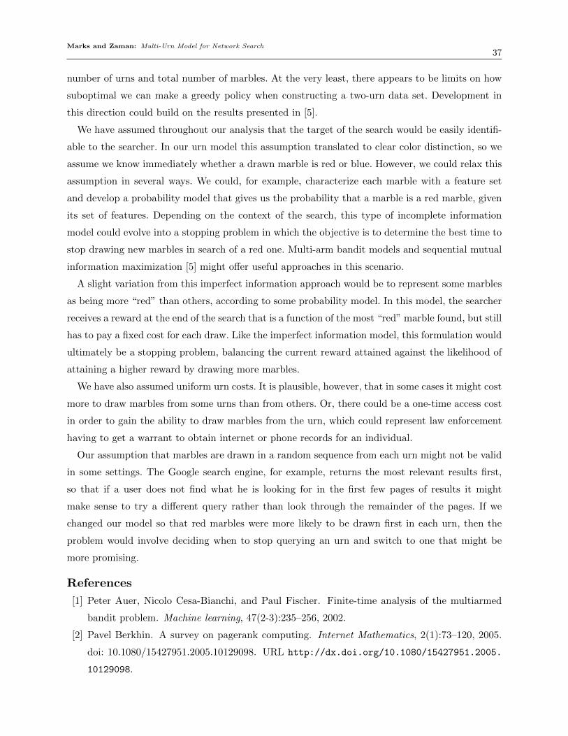
Marks and Zaman: Multi-Urn Model for Network Search37

number of urns and total number of marbles. At the very least, there appears to be limits on how

suboptimal we can make a greedy policy when constructing a two-urn data set. Development in

this direction could build on the results presented in [5].

We have assumed throughout our analysis that the target of the search would be easily identifi-

able to the searcher. In our urn model this assumption translated to clear color distinction, so we

assume we know immediately whether a drawn marble is red or blue. However, we could relax this

assumption in several ways. We could, for example, characterize each marble with a feature set

and develop a probability model that gives us the probability that a marble is a red marble, given

its set of features. Depending on the context of the search, this type of incomplete information

model could evolve into a stopping problem in which the objective is to determine the best time to

stop drawing new marbles in search of a red one. Multi-arm bandit models and sequential mutual

information maximization [5] might offer useful approaches in this scenario.

A slight variation from this imperfect information approach would be to represent some marbles

as being more “red” than others, according to some probability model. In this model, the searcher

receives a reward at the end of the search that is a function of the most “red” marble found, but still

has to pay a fixed cost for each draw. Like the imperfect information model, this formulation would

ultimately be a stopping problem, balancing the current reward attained against the likelihood of

attaining a higher reward by drawing more marbles.

We have also assumed uniform urn costs. It is plausible, however, that in some cases it might cost

more to draw marbles from some urns than from others. Or, there could be a one-time access cost

in order to gain the ability to draw marbles from the urn, which could represent law enforcement

having to get a warrant to obtain internet or phone records for an individual.

Our assumption that marbles are drawn in a random sequence from each urn might not be valid

in some settings. The Google search engine, for example, returns the most relevant results first,

so that if a user does not find what he is looking for in the first few pages of results it might

make sense to try a different query rather than look through the remainder of the pages. If we

changed our model so that red marbles were more likely to be drawn first in each urn, then the

problem would involve deciding when to stop querying an urn and switch to one that might be

more promising.

References

[1] Peter Auer, Nicolo Cesa-Bianchi, and Paul Fischer. Finite-time analysis of the multiarmed

bandit problem. Machine learning, 47(2-3):235–256, 2002.

[2] Pavel Berkhin. A survey on pagerank computing. Internet Mathematics, 2(1):73–120, 2005.

doi: 10.1080/15427951.2005.10129098. URL http://dx.doi.org/10.1080/15427951.2005.

10129098.

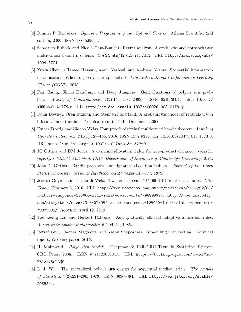
Marks and Zaman: Multi-Urn Model for Network Search38

[3] Dimitri P. Bertsekas. Dynamic Programming and Optimal Control. Athena Scientific, 2nd

edition, 2000. ISBN 1886529094.

[4] Sebastien Bubeck and Nicolo Cesa-Bianchi. Regret analysis of stochastic and nonstochastic

multi-armed bandit problems. CoRR, abs/1204.5721, 2012. URL http://arxiv.org/abs/

1204.5721.

[5] Yuxin Chen, S Hamed Hassani, Amin Karbasi, and Andreas Krause. Sequential information

maximization: When is greedy near-optimal? In Proc. International Conference on Learning

Theory (COLT), 2015.

[6] Fan Chung, Shirin Handjani, and Doug Jungreis. Generalizations of polya’s urn prob-

lem. Annals of Combinatorics, 7(2):141–153, 2003. ISSN 0219-3094. doi: 10.1007/

s00026-003-0178-y. URL http://dx.doi.org/10.1007/s00026-003-0178-y.

[7] Doug Downey, Oren Etzioni, and Stephen Soderland. A probabilistic model of redundancy in

information extraction. Technical report, DTIC Document, 2006.

[8] Esther Frostig and Gideon Weiss. Four proofs of gittins’ multiarmed bandit theorem. Annals of

Operations Research, 241(1):127–165, 2016. ISSN 1572-9338. doi: 10.1007/s10479-013-1523-0.

URL http://dx.doi.org/10.1007/s10479-013-1523-0.

[9] JC Gittins and DM Jones. A dynamic allocation index for new-product chemical research.

report), CUED/A-Mat Stud/TR13, Department of Engineering, Cambridge University, 1974.

[10] John C Gittins. Bandit processes and dynamic allocation indices. Journal of the Royal

Statistical Society. Series B (Methodological), pages 148–177, 1979.

[11] Jessica Guynn and Elizabeth Weis. Twitter suspends 125,000 ISIL-related accounts. USA

Today, February 6, 2016. URL http://www.usatoday.com/story/tech/news/2016/02/05/

twitter-suspends-125000-isil-related-accounts/79889892/. http://www.usatoday.

com/story/tech/news/2016/02/05/twitter-suspends-125000-isil-related-accounts/

79889892/; Accessed April 12, 2016.

[12] Tze Leung Lai and Herbert Robbins. Asymptotically efficient adaptive allocation rules.

Advances in applied mathematics, 6(1):4–22, 1985.

[13] Retsef Levi, Thomas Magnanti, and Yaron Shaposhnik. Scheduling with testing. Technical

report, Working paper, 2016.

[14] H. Mahmoud. Polya Urn Models. Chapman & Hall/CRC Texts in Statistical Science.

CRC Press, 2008. ISBN 9781420059847. URL https://books.google.com/books?id=

7Bizo28c2LQC.

[15] L. J. Wei. The generalized polya’s urn design for sequential medical trials. The Annals

of Statistics, 7(2):291–296, 1979. ISSN 00905364. URL http://www.jstor.org/stable/

2958811.