Information Sciences 381 (2017) 322–340

Contents lists available at ScienceDirect

Information Sciences

journal homepage: www.elsevier.com/locate/ins

A multi-criteria perception-based strict-ordering algorithm for

identifying the most-preferred choice among

equally-evaluated alternatives

Madjid Tavana

a , b , ∗, Debora Di Caprio

c , d , Francisco J. Santos-Arteaga

e , f

a Business Systems and Analytics Department, Distinguished Chair of Business Analytics, La Salle University, Philadelphia, PA 19141, USA b Business Information Systems Department, Faculty of Business Administration and Economics, University of Paderborn, D-33098

Paderborn, Germany c Department of Mathematics and Statistics, York University, Toronto M3J 1P3, Canada d Polo Tecnologico IISS G. Galilei, Via Cadorna 14, 39100 Bolzano, Italy e School of Economics and Management, Free University of Bolzano, 39100 Bolzano, Italy f Instituto Complutense de Estudios Internacionales, Universidad Complutense de Madrid, Campus de Somosaguas, 28223 Pozuelo, Spain

a r t i c l e i n f o

Article history:

Received 17 October 2015

Revised 21 August 2016

Accepted 26 November 2016

Available online 29 November 2016

Keywords:

Decision analysis

Multi-attribute alternative

Consumer indecision

Subjective perception

Lexicographic choice

Ordinal ranking

Expected utility

a b s t r a c t

Indecision constitutes a frequent and significant problem among decision makers (DMs).

The substantial amount of potential choices available, the subjectivity and imprecision in-

herent in the information received, and the limited capacity of DMs to assimilate the in-

formation available are generally blamed for the resulting indecisiveness. We consider the

problem of a DM who must rank a set of alternatives in a way that there are no two alter-

natives equally ranked. Each alternative is quantitatively and qualitatively described by a

different information sender (IS). That is, the DM cannot observe the alternatives directly,

he has to subjectively infer and evaluate them on the basis of the information provided by

the ISs. The current paper introduces a novel algorithm that generates a strict order over

the alternatives when DMs cannot decide among them. The proposed algorithm defines a

lexicographic choice rule that is implementable over different evaluation loops. This algo-

rithm complements and extends previous research on subjective evaluations and exchange

reliability where the ISs–DMs interaction does not guarantee that DMs are able to make

a unique most-preferred choice. We illustrate how this algorithm can also be adapted to

account for the strategic manipulation of the information provided by the ISs and for dif-

ferent attitudes towards uncertainty on the side of the DMs.

© 2016 Elsevier Inc. All rights reserved.

1. Introduction

Decision makers (DMs) in general, and consumers in particular, have considerable problems making choices, i.e. deciding.

For example, consider a consumer interested in purchasing one or more bottles of wine from a set of wine bottles belonging

to different sellers, or the head manager of a corporation who must select one or more projects to finance from a set

∗ Corresponding author at: Business Systems and Analytics Department, Distinguished Chair of Business Analytics, La Salle University, Philadelphia, PA

19141, USA. Fax: + 1 267 295 2854.

E-mail addresses: tavana@lasalle.edu (M. Tavana), dicaper@mathstat.yorku.ca , debora.dicaprio@istruzione.it (D. Di Caprio), fsantosarteaga@unibz.it ,

fransant@ucm.es (F.J. Santos-Arteaga).

http://dx.doi.org/10.1016/j.ins.2016.11.021

0020-0255/© 2016 Elsevier Inc. All rights reserved.

M. Tavana et al. / Information Sciences 381 (2017) 322–340 323

of project portfolios proposed by different applicants. In both cases, the DM must rank the available alternatives without

observing/testing them directly, but on the basis of the descriptions provided by each seller or applicant. Moreover, since

the number of alternatives that can be purchased or financed depends on a budget, it is important for the DM to be able to

rank the alternatives without obtaining any ties between them.

Consumer indecision has attracted a great deal of attention in the last decades given the emergence and rapid diffusion

of online search and choice environments. This phenomenon has been traditionally blamed on the substantial amount of

potential choices available [46] , the subjectivity and imprecision inherent in the linguistic information received [59] , and

the limited capacity of consumers to assimilate and analyze all the information received and follow a utility maximizing

approach [49] .

The following academic disciplines related to this particular phenomenon have developed their respective approaches

and explanations:

a) Economics: Economists have provided potential explanations for the indecision observed among consumers form a deci-

sion theoretical perspective, given the direct violation of the expected utility axioms that such a phenomenon constitutes.

A common solution to the consumer indecision problem was the elimination of the completeness axiom when defining

the preference relations of DMs [13,18] . A similar formal approach relies on the ambiguity of the set of outcomes de-

rived from the choice, with the DM being indecisive among options when the probability distribution defined over the

outcomes is unknown [10] .

The main alternative to this normative approach was given by the bounded rationality hypothesis [48] , according to

which DMs follow a heuristic rule when making their decisions [9] . Different heuristic mechanisms can be defined based

on the subjective tradeoff that the DMs consider between the accuracy of their decisions and the cognitive effort required

[24,36] . The literature on bounded rationality has emphasized the use of heuristic rules based on the attributes of the

alternatives, with the DM considering a small set of alternatives but concentrating on a particular set of their attributes

[36] .

b) Psychology: Psychologists have also studied the consumer indecision problem but following quite a different approach.

The initial papers dealing with the indecision problem illustrated that DMs have a greater tendency to avoid choosing

when there is not a clear dominant alternative. Such a strategy is generally followed to avoid making and regretting

difficult tradeoffs [56] . At the same time, psychologists tend to associate indecisiveness with low decisional confidence

and distinct patterns in the information search behavior of DMs [35] . In particular, indecisive DMs tend to use larger

working memory resources to search for information [20] and follow a maximizing tendency in order to try to obtain

the best alternative rather than a simply good enough one [17] .

A different branch of the literature has focused on the emotional response to choice and its effect on the happiness

of DMs [4,46] . In this case, potential regrets and selection difficulties are considered among the main factors generating

consumer indecision. Particular attention has been given to the difficulties that DMs face when performing a trade-off

between two alternatives and none of them is clearly superior to the other on all its characteristics [31] . In this regard,

Beattie and Barlas [8] illustrated the significant differences in the ease with which DMs can compare and decide between

different types of attributes. They also observed a lexicographic choice rule determining the DMs’ preference between

different attribute categories and proved the existence of regularities indicating when indifference and indecision could

arise.

Finally, this literature has emphasized the fact that product knowledge is highly subjective and based on the perception

capacity of the consumer. For example, Johnson et al. [28] used attitude theory to argue that the subjectively perceived

value of a product, i.e. an overall evaluation of the performance of the product given its price, has a more direct in-

fluence on the decision of the DMs when they are gathering information, forming their opinions, and trying to reduce

risk.

c) Information science: Information scientists have consistently highlighted the imprecision existing in the linguistic descrip-

tions of the different characteristics of the alternatives provided by the information senders (ISs). The application of fuzzy

sets [59] and, in particular, intuitionistic fuzzy sets [5,52] to emphasize the imprecision in the language used by the ISs

has led to the development of fuzzy variants of the standard models considered in the decision making literature [2,3] .

We will both acknowledge and account for the formalizations implemented by information theorists and their fuzzy

approach to decision making when designing the algorithms introduced through the paper. In particular, we will assume

that the DMs are aware of the existing differences in perception with respect to the ISs together with the imprecision

inherent to the description of each alternative.

1.1. Contribution

Consider a DM endowed with a limited capacity to process and assimilate information while facing a choice environ-

ment composed by multiple alternatives about whose characteristics he receives quantitative and qualitative information

from different ISs. As illustrated in the previous section, this DM may be unable to decide which one among the avail-

able alternatives to choose. The main contribution of the current paper is the introduction of a novel algorithm that gen-

erates a strict order over the alternatives when DMs are unable to decide among them. More precisely, this algorithm

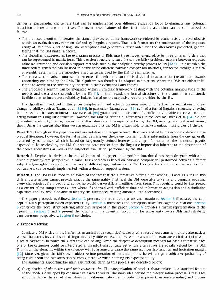
324 M. Tavana et al. / Information Sciences 381 (2017) 322–340

defines a lexicographic choice rule that can be implemented over different evaluation loops to eliminate any potential

indecision arising among alternatives. The main novel features of the strict-ordering algorithm can be summarized as

follows:

• The proposed algorithm integrates the standard expected utility framework considered by economists and psychologists

within an evaluation environment defined by linguistic reports. That is, it focuses on the construction of the expected

utility of DMs from a set of linguistic descriptions and generates a strict order over the alternatives presented, guaran-

teeing that the DM makes a choice. • The algorithm disaggregates the evaluation process of DMs into three stages, giving place to three different orders that

can be represented in matrix form. This decision structure relaxes the compatibility problems existing between expected

value maximization and decision support methods such as the analytic hierarchy process (AHP) [42,44] . In particular, the

three orders generated can be used to define three different pairwise comparison matrices, connected through a matrix

of weights determining the subjective importance assigned by the DM to each ranking. • The pairwise comparison process implemented through the algorithm is designed to account for the attitude towards

uncertainty exhibited by the DMs. The algorithm can therefore be adapted to situations where the DMs are either indif-

ferent or averse to the uncertainty inherent in their evaluations and choices. • The proposed algorithm can be integrated within a strategic framework dealing with the potential manipulation of the

reports and descriptions provided by the ISs [1] . In this regard, the formal structure of the algorithm is sufficiently

flexible so as to incorporate reliability indexes based on the subjective reports provided by the ISs.

The algorithm introduced in this paper complements and extends previous research on subjective evaluations and ex-

change reliability such as Tavana et al. [53,54] . In particular, Tavana et al. [53] defined a formal linguistic structure allowing

for the ISs and the DMs to interact. Tavana et al. [54] guaranteed the existence of a sufficiently reliable choice when inter-

acting within this linguistic structure. However, the ranking criteria of alternatives introduced by Tavana et al. [54] did not

guarantee decidability. That is, two or more alternatives could be equally ranked by the DM, making him indifferent among

them. Using the current algorithm we can guarantee that the DM is always able to make a unique most-preferred choice.

Remark 1. Throughout the paper, we will use notation and language terms that are standard to the economic decision the-

oretical literature. However, the formal setting defining our choice environment differs substantially from the one generally

assumed by economists, which is based on exogenously defined lotteries and crisp information on the numerical payoffs

expected to be received by the DM. Our setting accounts for both the linguistic imprecision inherent to the description of

the choice alternatives as well as the subjective evaluations performed by the DM.

Remark 2. Despite the decision theoretical format of the paper, the algorithm introduced has been designed with a de-

cision support system perspective in mind. Our approach is based on pairwise comparisons performed between different

subjectively-weighted expected alternatives at different aggregation levels. The lexicographic choice rule that results from

our analysis can be easily implemented within a decision support system.

Remark 3. The DM is assumed to be aware of the fact that the alternatives offered differ among ISs and, as a result, two

different alternatives cannot provide exactly the same utility. That is, if the DM were able to verify and compare each and

every characteristic from each alternative, he would derive different utilities from them. This requisite could be interpreted

as a variant of the completeness axiom where, if endowed with sufficient time and information acquisition and assimilation

capacities, the DM would be able to identify the differences existing among all the alternatives.

The paper proceeds as follows. Section 2 presents the main assumptions and notations. Section 3 illustrates the con-

cept of DM’s perception-based expected utility. Section 4 introduces the perception-based lexicographic relations. Section

5 constructs the novel strict ordering algorithm proposed in the paper. Section 6 provides a matrix representation of the

algorithm. Sections 7 and 8 present the variants of the algorithm accounting for uncertainty averse DMs and reliability

considerations, respectively. Section 9 concludes.

2. Proposed setting

Consider a DM with a limited information assimilation (cognitive) capacity who must choose among multiple alternatives

whose characteristics are described linguistically by different ISs. The DM will be assumed to associate each description with

a set of categories to which the alternative can belong. Given the subjective description received for each alternative, each

one of the categories could be interpreted as an intuitionistic fuzzy set whose alternatives are equally valued by the DM.

That is, all the elements within the category will be assumed to share the same membership function and hesitation margin

[52] . Moreover, given the DM’s own subjective interpretation of the descriptions, he will assign a subjective probability of

being right about the categorization of each alternative when defining his expected utility.

The arguments supporting the main assumptions defining this process are described below:

a) Categorization of alternatives and their characteristics: The categorization of product characteristics is a standard feature

of the models developed by consumer research theorists. The main idea behind the categorization process is that DMs

naturally divide the set of alternatives into different categories in order to improve their understanding and process

M. Tavana et al. / Information Sciences 381 (2017) 322–340 325

the information obtained from the environment [41,51] . In our setting, products will be subjectively incorporated into

categories by the DM based on their descriptions. That is, after receiving a (generally imprecise) linguistic description of

its characteristics, the DM assigns the product a set of categories to which it may belong.

An intuitive example justifying this assumption is given by the evaluations provided by several online service web-

sites such as TripAdvisor, where a five bullet ranking for different categories, as well as an overall ranking, are used

to evaluate a given alternative. DMs may observe the corresponding average values while having also access to ad-

ditional information, given by the description of the alternatives provided by previous DMs. The subjectivity and im-

precision of these linguistic descriptions has led to the emergence of new research lines such as opinion mining,

where the different, but related, words and phrases used by consumers to describe a product are categorized [27] . We

will return to the TripAdvisor evaluation framework in Section 5 , when illustrating the applicability of the proposed

algorithm.

b) Limited information processing capacity: The substantial information assimilation capacity assumed on the DMs when

making a choice has been widely acknowledged since the bounded rationality hypothesis was formally introduced in

the economic literature [48] . That is, there is a cognitive limit on the number of categories that a DM can consider

and manage when making a decision, even within everyday and not particularly complex choice contexts [45] . This is

also the case when choosing among alternatives that are perceived as similar by the DM [47] . Kahneman and Tversky

[29] provide an ample literature review of the information processing frictions that have been identified by psychologists

when analyzing consumer choice and economic rationality.

Decision engineers are also aware of the limited capacity of DMs to process and assimilate information. Consider, for

example, the evaluations provided by DMs in the AHP [43] . The DMs are asked to assign numerical values (together with

their reciprocals) taken from a basic integer scale in order to evaluate alternatives following a series of direct pairwise

comparisons. The limit on the capacity of DMs to analyze and assimilate all the necessary information is the basis for the

design of this and other types of decision support mechanisms. The compatibility between the strict-ordering algorithm

introduced in this paper and the AHP will be discussed in Section 6 .

c) Subjective perception and interpretation of information: The increasing recognition of the fact that the subjective perception

of the alternatives and their characteristics is a fundamental feature of the choice process of DMs has led cognitive sci-

ence to take over the economic rationality approach [7] . This switch between disciplines is mainly due to the additional

sophistication that cognitive science can provide to the analysis of the DM’s cognitive abilities and limitations [11] . For

example, cognitive research has shown how, when learning about different alternatives, the attention and memory pro-

cesses of the DM affect the perceived value of an alternative [50] . At the same time, perception varies between genders,

whose differences have been documented when analyzing online consumer reviews [6] .

Consider now the standard risky choices to which DMs are commonly subject in the behavioral economic literature

[29] . The choice of DMs between prospects has been shown to differ depending on whether the alternatives (probabilities

and outcome values) are given directly to them or they have inferred the corresponding values from experience [12] . That

is, subjective differences in the learning and experience capacities of the DMs determine their evaluation of the different

alternatives.

In summary, indecision may arise among DMs, particularly so when comparing similar alternatives that can be catego-

rized similarly. In this case, indecision arises due to the fuzzy characterization of the products and the subjective interpre-

tation of the probabilities assigned by the DMs, who have a limited capacity to assimilate and evaluate the information

available. Thus, as observed empirically, particularly so in online search and decision environments, indecision may quite

often characterize the outcome derived from the search and choice process of the DMs.

2.1. Assumptions

We consider the problem of a DM who must strictly rank n alternatives without the possibility of observing them di-

rectly. Each alternative is described by a different information sender (IS). We assume that the DM checks a certain amount

of information about each alternative and that this information is given in the form of a list of evaluations corresponding to

certain (or all) characteristics composing the alternative.

We assume the characteristics of an alternative to be describable by either quantitative (objective) or qualitative (subjec-

tive) evaluations. Quantitative evaluations are usually given in terms of numerical values and can be assumed to vary within

a real interval. Qualitative evaluations are descriptions in plain language and the best way of formalizing them is through

linguistic variables and fuzzy numbers [37] . For instance, in the case of a consumer buying a bottle of wine, the charac-

teristics of an alternative include %vol, price, color, flavor, smell , etc. Some of the characteristics are quantitative (i.e., %vol,

price ), while others are qualitative (i.e., color, flavor, smell ). Similarly, in the case of a head manager selecting a project, the

alternatives present quantitative characteristics, such as cost, time, manpower , and qualitative characteristics, such as quality

and reliability .

We assume the DM and the ISs to have a subjective (and generally different) perception of the characteristics of an

alternative. Thus, they do not necessarily value the qualitative characteristics of the same alternative in the same way. The

326 M. Tavana et al. / Information Sciences 381 (2017) 322–340

order in which the characteristics are described also differs in general from person to person, but we do not need to consider

this fact explicitly since it will not affect our results.

Remark 4. Note that if the DM checks the values of all the characteristics of an alternative, then he necessarily collects

qualitative information. If the DM does not check the values of all the characteristics of an alternative, then he may or may

not collect qualitative information. In the last case, the DM may think of more than one alternative endowed with the same

quantitative characteristics. Therefore, in all cases, the DM is forced to interpret the information acquired and put together

a set of alternatives matching the description provided by the ISs from his own viewpoint.

Finally, we endow the DM with a preference relation on the set of all the existing alternatives. A preference relation on

a finite set of alternatives is a binary relation satisfying reflexivity, completeness and transitivity. Preference relations on

finite sets are represented by utility functions, that is, increasing real-valued functions on the set of alternatives by means

of which the DM assigns to each alternative a value measuring its importance. We assume that the utility function defined

by the DM takes only positive integer values.

2.2. Basic notions and notations

For the sake of completeness, we include below the properties of a binary relation and the definitions of the order

relations that we will refer to in the following sections. We mainly refer to Fishburn [21] , Engelking [19] and Munkres

[33] for the definitions regarding order relations. We follow Osborne and Rubinstein [34] and Mas-Colell et al. [32] for

concepts related to preference relations

Let P be a nonempty set and R be a binary relation on P .

Reflexivity : ∀ p ∈ P, p R p

Irreflexivity : ∀ p ∈ P, p R p does not hold

Antisymmetry : ∀ p, p ’ ∈ P, p R p ’ and p ’ R p ⇒ p = p ’

Transitivity : ∀ p, p ’, p ” ∈ P, p R p ’ and p ’ R p ” ⇒ p R p ”

Comparability ( weak connectedness ): ∀ p , p ’ ∈ P, p � = p ’ ⇒ either p R p ’ or p ’ R p

Completeness : ∀ p , p ’ ∈ P, p R p ’ or p ’ R p (possibly both)

The binary relation R defines on P a

• preference relation if it satisfies reflexivity, completeness and transitivity; • strict preorder (or strict partial order ) if it satisfies irreflexivity and transitivity; • partial order if it satisfies reflexivity, antisymmetry and transitivity; • preorder (or quasiorder ) if it satisfies reflexivity and transitivity; • linear order (or strict order , or strict preference relation ) if it satisfies irreflexivity, transitivity and comparability.

Note that strict preference relations are linear orders. Also, preference relations are complete preorders.

Two elements p and p ’ of an ordered set can be incomparable , that is, it can happen that neither p R p ’ nor p ’ R p holds.

It is clear that a strict ranking of a set of alternatives can be created if and only if a linear order (equivalently, a strict

preference relation) can be defined on it.

Assuming a preference relation on the DM allows him to be a priori indifferent between two or more alternatives. Hence,

it also entails the use of equivalence classes with respect to the indifference relation induced by the given preference rela-

tion. These equivalence classes can be assigned a strict preference order and strictly increasing utility values.

We formalize our assumptions through the following notations:

D the DM

n a fixed, but arbitrary, integer value

S i the i th IS; i = 1, …, n

G the set of all existing alternatives

A i the alternative described by ; i = 1, …, n

� the set of the n alternatives offered by the ISs, that is: �= { A 1 , …, A n }

� the set of all the possible characteristics of any alternative in G

| �| the cardinality of the set �

X δ the set of all values that S i can assign to the δth characteristic of A i ; δ ∈ �

x i δ[ A i ] the value in X δ that S i assigns to the δth characteristic of A i ; δ ∈ �, i = 1, …, n

x D δ

[ g] the value in X δ that D would assign to the δth characteristic of the generic alternative g in G ; δ ∈ �

J i the set of characteristics of A i actually checked by D or described by S i ; J i ⊆�, i = 1, …, n

= D the equality relation from the point of view of D

x D δ

[ g] = D x δ means that D assigns the value x δ to the δth characteristic of g in G

R the set of real numbers

≥ the standard partial order on the set R

M. Tavana et al. / Information Sciences 381 (2017) 322–340 327

> the standard linear order on the set R

� the preference relation that D defines on G , that is, � is a reflexive, complete and transitive binary relation on

G

≈ the indifference relation induced by � on G , that is, ∀ g, g ’ ∈ G, g ≈ g ’ ⇔ g � g ’ and g ’ � g .

U the utility function defined by D on the set of all existing alternatives G , that is, U: G → R such that ∀ g, g ’ ∈ G,

g � g ’ ⇔ U ( g ) ≥ U ( g ’)

�=G / ≈ the set of equivalence classes with respect to the indifference relation ≈ . Henceforth, we will refer to the

equivalence classes in � as “categories”.

˜ g the equivalence class in � to which the alternative g belongs; that is: ˜ g = [ g] ≈ = { g ′ ∈ G : g ′ ≈ g} = { g ′ : U(g ′ ) =U(g) }

the induced strict preference relation that D defines on �; satisfies irreflexivity, comparabilty and transitivity

u the induced utility function defined by D on the set of equivalence classes �, that is, the strictly increasing real-

valued function u : �→ R defined by: ∀ g ∈ �, u ( g ) = U(g) .

3. DM’s perception-based expected utility

Given the setting introduced in the previous section, for every i = 1, …, n, D checks the values assigned by S i to the

characteristics of A i belonging to a fixed subset J i of �. After collecting this information from the i th IS, D envisions one

or more alternatives among those in G (see Remark 4 ), but none of these alternatives need to coincide with the actual

one described by S i , namely A i . More precisely, as a consequence of the fact that D subjectively interprets the description

provided by S i , the following two cases are possible:

• D thinks that S i is describing a certain subset of G and this subset actually contains A i , • D thinks that S i is describing a certain subset of G , but this subset does not contain A i .

Furthermore, in order to account for the possibility of obtaining alternatives equivalent to those envisioned, D should

consider the categories to which the envisioned alternatives belong instead of the single alternatives. To formalize this idea

of envisioned alternatives/categories, we build on the models proposed by Tavana et al. [53,54] and introduce the “perceived

possibility sets”, that is, the sets of categories that the DM considers after collecting the information from the ISs.

Definition 1. For every i = 1, …, n , let � i be the set of all the categories that D envisions after checking the values assigned

by S i to the characteristics in J i . In symbols, we have:

�i =

{˜ g ∈ � : ∀ δ ∈ J i , x D δ [ g] = D x

i δ[ A i ]

}(1)

We will refer to � i as the perceived possibility set induced by S i on D .

In other words, each set � i corresponds to the set of categories that D believes to be compatible with the information

obtained from S i . Recall that x D δ

[ g] = D x i δ[ A i ] means that D assigns the value x i

δ[ A i ] to the δth characteristic of the generic

alternative g (see Section 2.2 ). The following example shows how D constructs the perceived possibility set induced by an IS.

Example 1. Suppose that the set of all existing alternatives consists of nine elements, that is, G = { a, b, c, d, e, f, g, h, k } and

that D defines the following utility on the set G :

U(a ) = 2 , U(b) = 3 , U(c) = 5 , U(d) = 3 , U(e ) = 7 , U( f ) = 2 , U(g) = 3 , U(h ) = 7 , U(k ) = 3 .

Then, � = G/ ≈ = { a , ˜ b , ˜ c , ˜ e } , where:

˜ a = { a, f } , ˜ b = { b, d, g, k } , ˜ c = { c} , ˜ e = { e, h } . Suppose that the IS S i assigns to the characteristics δ( quantitative ), σ ( qualitative ) and θ ( quantitative ) of the alternative A i

(that is, J i ={ δ, σ , θ}) the following values:

x i δ[ A i ] = 10 0 0 , x i σ [ A i ] = v ery good, x i θ [ A i ] = 30 .

Finally, suppose that D assigns the following values to the same characteristics of the categories in �:

x D δ [ a ] = 10 0 0 , x D σ [ a ] = v ery good, x D θ [ a ] = 30 ,

x D δ [ b] = 10 0 0 , x D σ [ b] = regular, x D θ [ b] = 12 ,

x D δ [ c] = 800 , x D σ [ c] = v ery good, x D θ [ c] = 45 ,

x D δ [ e ] = 10 0 0 , x D σ [ e ] = v ery good, x D θ [ e ] = 30 .

Then, after checking the evaluations provided by S i , D thinks that S i is describing an alternative belonging to either ˜ a the

category or the category ˜ e . That is, � = { a , e } .

i

328 M. Tavana et al. / Information Sciences 381 (2017) 322–340

Table 1

Some cases allowed/not allowed by Requirement 2 when � i =� j .

Information sender S i Information sender S j

Allowed

Alternatives envisioned by D after receiving information a, b, c

U(a ) = 8 , U(b) = 6 , U(c) = 4

d, e, f

U(d) = 8 , U(e ) = 6 , U( f ) = 4 .

Perceived possibility sets and D ’s utilities �i = { a , ˜ b , ˜ c } = � j

u ( a ) = 8 , u ( b ) = 6 , u ( c ) = 4

D ’s subjective beliefs p i ( a ) =

1 2 , p i ( b ) =

1 4 , p i ( c ) =

1 4

, p j ( a ) =

1 4 , p j ( b ) =

1 4 , p j ( c ) =

1 2

Not allowed

Alternatives envisioned by D after receiving information a, b, c

U(a ) = 8 , U(b) = 6 , U(c) = 4

d, e, f

U(d) = 8 , U(e ) = 6 , U( f ) = 4

Perceived possibility sets and D ’s utilities �i = { a , b , c } = � j

u ( a ) = 8 , u ( b ) = 6 , u ( c ) = 4

D ’s subjective beliefs p i ( a ) =

1 2 , p i ( b ) =

1 4 , p i ( c ) =

1 4

, p j ( a ) =

1 2 , p i ( c ) =

1 4 , p j ( c ) =

1 4

,

Not allowed

Alternatives envisioned by D after receiving information a

U(a ) = 8

d

U(d) = 8

Perceived possibility sets and D ’s utilities �i = { a } = � j

u ( a ) = 8 .

D ’s subjective beliefs p i ( a ) = 1 p j ( a ) = 1

Note that D naturally defines a strict preference relation on each set of the form � i by considering the restriction of to � i . Thus, we can assume that D orders the categories in � i from the most to the least important one from his viewpoint

and enumerates them accordingly.

This translates in the following consistency requirement.

Requirement 1. For every i = 1, …, n , D enumerates the alternatives in � i from the most to the least preferred one, that

is: �i = { a i 1 , ˜ a i 2 , . . . , ˜ a i # i } and ˜ a i 1 ˜ a i 2 · · · ˜ a i # i , where #

i denotes the cardinality of � i .

By Definition 1 , it follows that D faces the uncertainty deriving from the fact that he cannot be sure of which category

among those in � i is actually the one containing the alternative offered by S i or even if this category is really in � i .

Nevertheless, following Tavana et al. [53,54] , we can assume D to have subjective beliefs about which category in � i is more

probable to be the one containing the alternative offered by S i . Thus, we endow D with a family of probability functions,

one per each set and, hence, per each IS.

Definition 2. For every i = 1, …, n , , let p i : � i → [0, 1] be the subjective probability function defined by D on � i such that,

for every, the value p i ( g ) is the probability assigned by to ˜ g actually being the category of the alternative described by S i .

The n alternatives that the DM must rank are clearly assumed to be pairwise different for the DM, but nothing prevents

the fact that two or more of them could belong to the same category. This fact must somehow be reflected in the way

in which the DM perceives them. In particular, the perceived possibility sets should either be pairwise different or be as-

signed different probability functions. That is, following Remark 3 , the DM acknowledges the fact that the alternatives differ

among ISs and two different alternatives cannot provide the same utility. Thus, we must also add the following consistency

requirement.

Requirement 2. ∀ i, j ∈ {1, …, n }, i � = j ⇒ � i � = � j or ( � i =� j and ∃ g ∈ �i : p i ( g ) � = p j ( g ) ).

Remark 5. Requirement 2 excludes from our analysis all cases where ∃ i, j ∈ {1, …, n }, with i � = j , such that � i =� j and

p i =p j (as functions). In particular, the case where �i = { a } = � j for some i, j ∈ {1, …, n }, with i � = j , is not allowed. Indeed,

in this case, the DM is obliged to define the same probability function on � i and � j , that is, p i ( a ) = 1 = p j ( a ) . Table 1

describes some instances allowed/not allowed by Requirement 2 when � i =� j .

Remark 6. Throughout the paper, we will provide several numerical examples some of which assume a considerably wide

domain when determining the number of categories and their corresponding utilities. However, as illustrated in the litera-

ture review section, (cognitively constrained) DMs usually generate a lower number of categories, giving place to frequent

ties in expected utility terms between alternatives.

Similarly to Tavana et al. [53,54] , Definitions 1 and 2 allow us to introduce a perception-based variant of the expected

utility that D associates to each of the available alternatives. The expected utility of the alternative A i is the utility that D

expects from choosing A i . We define this expected utility as follows.

Definition 3. For every i = 1, …, n , the perception-based expected utility that D assigns to A i is given by the following sum:

E(u, p i ) =

∑

˜ g ∈ �i

u ( g ) · p i ( g ) . (2)

M. Tavana et al. / Information Sciences 381 (2017) 322–340 329

Table 2

Perceived possibility sets, utilities and subjective beliefs of D in Example 2.

Information sender S 1 Information sender S 2

Perceived possibility set induced by S i �1 = { b , ˜ c , ˜ d }

˜ b ˜ c ˜ d

�2 = { a , ˜ b , ˜ e , ˜ f } ˜ a ˜ b ˜ e ˜ f

D ’s utilities u ( b ) = 16 , u ( c ) = 14 , u ( d ) = 12 u ( a ) = 28 , u ( b ) = 16 ,

u ( e ) = 8 , u ( f ) = 4

D ’s subjective beliefs p 1 ( b ) = p 1 ( d ) =

1 4 , p 1 ( c ) =

1 2

p 2 ( a ) = p 2 ( b ) = p 2 ( e ) = p 2 ( f ) =

1 4

Definition 3 naturally yields the following.

Definition 4. We denote by ≺E the binary relation on � defined as follows.

∀ A i , A j ∈ �, A i ≺E A j de f ←→ E(u, p i ) < E(u, p j ) . (3)

The relation ≺E can be used to define a preference relation for D on the set �, that is:

A i ≺E A j de f ←→ A i ≺E A j or A i ≈E A j

←→ E(u, p i ) < E(u, p j ) or E(u, p i ) = E(u, p j ) . (4)

However, ≺E is not a strict preference relation for D on �. Indeed, two distinct alternatives A i and A j in � can produce

the same perception-based expected utility value, which means that D can be indifferent between these two alternatives

and, hence, rank them equally.

Example 2. Suppose that D must rank two alternatives, A 1 and A 2 , belonging to S 1 and S 2 , respectively. Suppose that, on

the basis of the description provided by S 1 and S 2 , D thinks that S 1 is describing one of the alternatives in { b , c , d }, where

U ( b ) > U ( c ) > U ( d ), while S 2 is describing one of the alternatives in { a , b , e , f }, where U ( a ) > U ( b ) > U ( e ) > U ( f ). Then,

�1 = { b , ˜ c , ˜ d } , where ˜ b ˜ c ˜ d , and �2 = { a , ˜ b , ˜ e , ˜ f } , where ˜ a ˜ b ˜ e ˜ f . Note that A 1 and A 2 may or may not be among

those alternatives envisioned by D , but this fact does not influence the ranking. Let the utilities and subjective beliefs of D

be defined as in Table 2 . Then, E ( u , p 1 ) = E ( u , p 2 ) = 14, so that D is unable to decide between A 1 and A 2 .

Therefore, ≺E does not always allow D to compare and strictly rank two different options. We can express this fact

formally using the following definition and proposition.

Definition 5. Let A i , A j ∈ �, with i � = j . We say that A i and A j are E-comparable for D , if D is not indifferent between them

(i.e. either A i ≺E A j or A j ≺E A i ).

Proposition 1. The binary relation ≺E satisfies irreflexivity and transitivity, but not comparability. Hence, ≺E is a strict

preorder, but not a linear order, on �. In particular, two different alternatives in � are not necessarily E-comparable for

D .

In the next section, we introduce two new order relations that, together with ≺E , will be used to define a composite

linear order on �. This linear order will allow D to obtain a strict ranking of the alternatives.

4. Introducing perception-based lexicographic relations

We now introduce two new binary relations on the set � of the n available alternatives. Each of these relation induces

a notion of comparability/incomparability on �. Afterwards, we will show that, as it is the case for ≺E , these relations on

their own are not enough to guarantee a “strict comparison” between two alternatives in �. How these relations and ≺E

can be combined together in an algorithmic way so as to produce a strict preference relation on � will be shown in the

next section.

In order to define the new order relations additional notations are required.

For every i = 1, …, n , let

� L ( �i ) = (u ( a i 1 ) p i ( a i 1 ) , u ( a i 2 ) p i ( a i 2 ) , . . . , u ( a i # i ) p i ( a i # i )) (5)

For every i = 1, …, n and every positive integer ε, let

� L ( �i | ε) =

{(u ( a i 1 ) p i ( a i 1 ) , u ( a i 2 ) p i ( a i 2 ) , . . . , u ( a iε ) p i ( a iε )) i f ε < # i � L ( �i ) i f ε ≥ # i

(6)

Both

� L ( �i ) and

� L ( �i | ε) are ordered tuples of real values. In particular, � L ( �i | ε) is the restriction of � L ( �i ) to its first ε

coordinates. Given i � = j , both

� L ( �i | ε) and

� L ( � j | ε) consist of ε coordinates and, hence, it is possible to order them lexico-

graphically. We exploit this fact to introduce the following relation on �.

330 M. Tavana et al. / Information Sciences 381 (2017) 322–340

�

�

Definition 6. We denote by ≺� L the binary relation on � defined as follows.

∀ A i , A j ∈ �, A i ≺� L A j

de f ←→

� L ( �i | min { # i , # j } ) < Lex

� L ( � j | min { # i , # j } )

←→ ∃ s ∗ ≤ min { # i , # j } such that ∀ s < s ∗, u ( a is ) p i ( a is ) = u ( a js ) p j ( a js ) and u ( a ∗

is ) p i ( a ∗

is ) < u ( a ∗

js ) p j ( a ∗

js ) .

(7)

In other words, A i is less preferred than A j if the restricted ordered tuple � L ( �i | min { # i , # j } ) is smaller than the restricted

ordered tuple � L ( � j | min { # i , # j } ) w.r.t. the standard lexicographic order. This yields to the following comparability notion.

Definition 7. Let A i , A j ∈ �, with i � = j . We say that A i and A j are lexicographically comparable for D w.r.t his beliefs and

preferences on � i and � j (in short: L-comparable for D ), if either A i ≺� L A j or A j ≺�

L A i .

For every i = 1, …, n , let

� U ( �i ) = (u ( a i 1 ) , u ( a i 2 ) , . . . , u ( a i # i )) . (8)

For every i = 1, …, n and every positive integer ε, let

� U ( �i | ε) =

{(u ( a i 1 ) , u ( a i 2 ) , . . . , u ( a iε )) i f ε < # i � U ( �i ) i f ε ≥ # i

(9)

As above, given i � = j , both

� U ( �i | ε) and

� U ( � j | ε) consist of ε coordinates and, hence, it is possible to order them lexico-

graphically. Thus, we can introduce another relation on �.

Definition 8. We denote by ≺� U the binary relation on � defined as follows.

∀ A i , A j ∈ �, A i ≺� U A j

de f ←→

� U ( �i | min { # i , # j } ) < Lex

� U ( � j | min { # i , # j } )

←→ ∃ s ∗ ≤ min

{# i , # j

}such that

∀ s < s ∗, u ( a is ) = u ( a js ) and u ( a ∗is ) < u ( a ∗js ) . (10)

Definition 8 yields the following comparability notion.

Definition 9. Let A i , A j ∈ �, with i � = j . We say that A i and A j are lexicographically comparable for D w.r.t his preferences on

� i and � j (in short: U-comparable for D ), if either A i ≺� U A j or A j ≺�

U A i .

Proposition 2. The binary relations ≺� L and ≺�

U are strict preorders on �.

Proof. Irreflexivity : Both relations are trivially irreflexive.

Transitivity : Let i , j , h ∈ {1, …, n } be such that A i ≺� L A j and A j ≺�

L A h . Hence, there exists s ≤ min { # i , # j } such that

∀ s < s , u ( a is ) p i ( a is ) = u ( a js ) p j ( a js ) and u ( a i s ) p i ( a i s ) < u ( a j s ) p j ( a j s ) .

At the same time, there exists ˆ s ≤ min { # j , # h } such that

∀ s <

ˆ s , u ( a js ) p j ( a js ) = u ( a hs ) p h ( a hs ) and u ( a j s ) p j ( a j s ) < u ( a h s ) p h ( a h s ) .

Let s ∗ ≤ min { s , ˆ s } . Then,

∀ s < s ∗, u ( a is ) p i ( a is ) = u ( a js ) p j ( a js ) = u ( a hs ) p h ( a hs ) .

Moreover, if s ∗ = s , we have:

u ( a is ∗ ) p i ( a is ∗ ) < u ( a js ∗ ) p j ( a js ∗ ) = u ( a hs ∗ ) p h ( a hs ∗ )

while, if s ∗ = ˆ s , we have:

u ( a is ∗ ) p i ( a is ∗ ) = u ( a js ∗ ) p j ( a js ∗ ) < u ( a hs ∗ ) p h ( a hs ∗ ) .

This means that � L ( �i | min { # i , # h } ) < Lex � L ( �h | min { # i , # h } ) and, hence, A i ≺�

L A h .

Suppose now that i , j , h ∈ {1, …, n } are such that A i ≺� U A j and A j ≺�

U A h . Reasoning as above, we have� U ( �i | min { # i , # h } ) < Lex

� U ( �h | min { # i , # h } ) and, hence, A i ≺�

U A h . �

As in the case of ≺E , the binary relations ≺L and ≺U are not linear orders since they do not satisfy the comparability

property. That is, two different alternatives in � do not need to be L-comparable or U-comparable for D . We provide two

very simple examples showing this fact.

Example 3. Suppose that D must rank two alternatives A 1 and A 2 belonging to S 1 and S 2 , respectively. Let the per-

ceived possibility sets �1 and �2 , the utilities and the subjective beliefs of D be defined as in Table 3 . Then, L ( �1 | min { # 1 , # 2 } ) =

� L ( �1 | 2) = ( 14 · 1

2 , 8 · 1 2 ) = (7 , 4) and

� L ( �2 | min { # 1 , # 2 } ) =

� L ( �2 | 2) = ( 28 · 1

4 , 16 · 1 4 ) = (7 , 4) . Since,

L ( �1 | min { # 1 , # 2 } ) and

� L ( �2 | min { # 1 , # 2 } ) coincide, D cannot decide between A 1 and A 2 using the relation ≺L .

Example 4. Suppose that D must rank two alternatives A 1 and A 2 belonging to S 1 and S 2 , respectively. Let the perceived

possibility sets � and � , the utilities and the subjective beliefs of D be defined as in Table 4 . Clearly, � U ( � | min { # , # } )

1 2 1 1 2

M. Tavana et al. / Information Sciences 381 (2017) 322–340 331

Table 3

Perceived possibility sets, utilities and subjective beliefs of D in Example 3.

Information sender S 1 Information sender S 2

Perceived possibility set induced by S i �1 = { c , ˜ e } ˜ c ˜ e

�2 = { a , ˜ b , ˜ e , ˜ f } ˜ a ˜ b ˜ e ˜ f

D ’s utilities u ( c ) = 14 , u ( e ) = 8 , u ( a ) = 28 , u ( b ) = 16

u ( e ) = 8 , u ( f ) = 4 ,

D ’s subjective beliefs p 1 ( c ) = p 1 ( e ) =

1 2

p 2 ( a ) = p 2 ( b ) = p 2 ( e ) = p 2 ( f ) =

1 4

Table 4

Perceived possibility sets, utilities and subjective beliefs of D in Example 4.

Information sender S 1 Information sender S 2

Perceived possibility set induced by S i �1 = { a , ˜ b } ˜ a ˜ b

�2 = { a , ˜ b , ˜ e , ˜ f } ˜ a ˜ b ˜ e ˜ f

D ’s utilities u ( a ) = 28 , u ( b ) = 16 u ( a ) = 28 , u ( b ) = 16

u ( e ) = 8 , u ( f ) = 4 ,

D ’s subjective beliefs p 1 ( a ) = p 1 ( b ) =

1 2

p 2 ( a ) = p 2 ( b ) = p 2 ( e ) = p 2 ( f ) =

1 4

and

� U ( �2 | min { # 1 , # 2 } ) are both equal to (28, 16). Thus, D cannot decide between A 1 and A 2 using the relation ≺U . Note

that the beliefs of the DM do not play any role when using the relation ≺U .

Note how one of the perceived possibility sets in Example 4 is the “initial segment” of the other. Namely, the elements of

�1 coincide with the first # 1 elements of �2 . Thus, Example 4 also shows that two alternatives A i and A j such that � i ⊂� j

and � i consists of the first # i elements of � j do not need to be U-comparable. As we will show in the following section, to

guarantee U-compatibility we need to impose a somehow complementary condition on the perceived possibility sets.

Henceforth, we will write �i = � j ‖ # i to indicate the fact that � i is the initial segment of � j of length # i .

5. Strict ordering algorithm

We start by showing that two different alternatives in � are either E-comparable or, if not, they are necessarily L-

comparable for D whenever the corresponding perceived possibility sets coincide or one is the initial segment of the other.

This provides a first condition to guarantee comparability when combing together the relations ≺E and ≺L . Afterwards, we

analyze the condition for ≺U to satisfy comparability.

Proposition 3. Let A i , A j ∈ �, with i � = j . Suppose that either � i =� j or �i = � j ‖ # i . Then, A i and A j are either E-comparable

or not E-comparable but L-comparable.

Proof. We need to consider two cases:

(a) If � i =� j , then # i = # j and ∀ s ≤ # i , ˜ a is = ˜ a js . By Requirement 2, the probability functions p i and p j must differ; thus

∃ s ∗ ≤ # i such that p i ( a is ∗ ) � = p j ( a js ∗ ) . (b) If �i = � j ‖ # i , then # i = min { # i , # j } and ∀ s ≤ # i , ˜ a is − ˜ a js . Since p i and p j have different supports, there must exist

s ∗ ≤ # i such that p i ( a is ∗ ) � = p j ( a js ∗ ) .

Clearly, in both cases (a) and (b), either E ( u , p i ) � = E ( u , p j ) or E ( u , p i ) = E ( u , p j ). If E ( u , p i ) � = E ( u , p j ), A i and A j

are E-comparable. If E ( u , p i ) = E ( u , p j ), then ∃ s ∗ ≤ # i such that ∀ s < s ∗, u ( a is ) p i ( a is ) = u ( a js ) p j ( a js ) and u ( a is ∗ ) p i ( a is ∗ ) � =u ( a js ∗ ) p j ( a js ∗ ) , which implies that A i and A j are L-comparable. �

For every positive integer λ, let

�λ = { A i ∈ � : # i = λ} . (11)

In our framework, for every i −1, …, n, S i describes A i by providing information about a certain set of characteristics,

J i , and, based on this information, D puts together the set � i of all the categories that he thinks could correspond to A i .

Thus, �λ is the subset of � containing the alternatives A i whose corresponding perceived possibility set � i consists of λelements.

The next proposition shows that the relation ≺� U is actually a linear order when restricted to subsets of � of the form

�λ whose elements are pairwise different. That is, two alternatives A i and A j in � are U-comparable for the DM if, after

receiving the information from S i and S j , he envisions the same number of categories but not the same categories.

Proposition 4. Let λ be a positive integer such that �λ � = ∅ . If ∀ A i , A j ∈ �λ, � i � = � j , then the restriction of the binary

relation ≺�

to �λ satisfies the comparability property.

U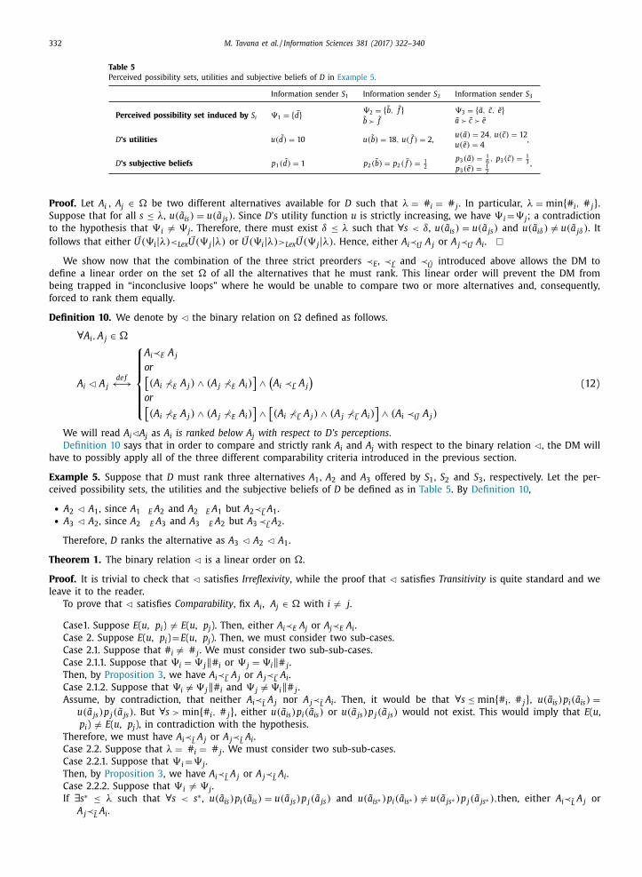

332 M. Tavana et al. / Information Sciences 381 (2017) 322–340

Table 5

Perceived possibility sets, utilities and subjective beliefs of D in Example 5.

Information sender S 1 Information sender S 2 Information sender S 3

Perceived possibility set induced by S i �1 = { d } �2 = { b , ˜ f } ˜ b ˜ f

�3 = { a , ˜ c , ˜ e } ˜ a ˜ c ˜ e

D ’s utilities u ( d ) = 10 u ( b ) = 18 , u ( f ) = 2 , u ( a ) = 24 , u ( c ) = 12

u ( e ) = 4 ,

D ’s subjective beliefs p 1 ( d ) = 1 p 2 ( b ) = p 2 ( f ) =

1 2

p 3 ( a ) =

1 6 , p 3 ( c ) =

1 3

p 3 ( e ) =

1 2

,

Proof. Let A i , A j ∈ � be two different alternatives available for D such that λ = # i = # j . In particular, λ = min { # i , # j } .Suppose that for all s ≤ λ, u ( a is ) = u ( a js ) . Since D ’s utility function u is strictly increasing, we have � i =� j ; a contradiction

to the hypothesis that � i � = � j . Therefore, there must exist δ ≤ λ such that ∀ s < δ, u ( a is ) = u ( a js ) and u ( a iδ ) � = u ( a jδ ) . It

follows that either � U ( �i | λ) < Lex � U ( � j | λ) or � U ( �i | λ) > Lex

� U ( � j | λ) . Hence, either A i ≺�

U A j or A j ≺� U A i . �

We show now that the combination of the three strict preorders ≺E , ≺� L and ≺U introduced above allows the DM to

define a linear order on the set � of all the alternatives that he must rank. This linear order will prevent the DM from

being trapped in “inconclusive loops” where he would be unable to compare two or more alternatives and, consequently,

forced to rank them equally.

Definition 10. We denote by � the binary relation on � defined as follows.

∀ A i , A j ∈ �

A i � A j de f ←→

⎧ ⎪ ⎪ ⎪ ⎪ ⎨

⎪ ⎪ ⎪ ⎪ ⎩

A i ≺E A j

or [( A i ⊀E A j ) ∧ ( A j ⊀E A i )

]∧

(A i ≺�

L A j

)or [( A i ⊀E A j ) ∧ ( A j ⊀E A i )

]∧

[( A i ⊀�

L A j ) ∧ ( A j ⊀� L A i )

]∧ ( A i ≺�

U A j )

(12)

We will read A i � A j as A i is ranked below A j with respect to D’s perceptions .

Definition 10 says that in order to compare and strictly rank A i and A j with respect to the binary relation � , the DM will

have to possibly apply all of the three different comparability criteria introduced in the previous section.

Example 5. Suppose that D must rank three alternatives A 1 , A 2 and A 3 offered by S 1 , S 2 and S 3 , respectively. Let the per-

ceived possibility sets, the utilities and the subjective beliefs of D be defined as in Table 5 . By Definition 10 ,

• A 2 � A 1 , since A 1 �E A 2 and A 2 �E A 1 but A 2 ≺� L A 1 .

• A 3 � A 2 , since A 2 �E A 3 and A 3 �E A 2 but A 3 ≺� L A 2 .

Therefore, D ranks the alternative as A 3 � A 2 � A 1 .

Theorem 1. The binary relation � is a linear order on �.

Proof. It is trivial to check that � satisfies Irreflexivity , while the proof that � satisfies Transitivity is quite standard and we

leave it to the reader.

To prove that � satisfies Comparability , fix A i , A j ∈ � with i � = j .

Case1. Suppose E ( u , p i ) � = E ( u , p j ). Then, either A i ≺E A j or A j ≺E A i .

Case 2. Suppose E ( u , p i ) = E ( u , p j ). Then, we must consider two sub-cases.

Case 2.1. Suppose that # i � = # j . We must consider two sub-sub-cases.

Case 2.1.1. Suppose that �i = � j ‖ # i or � j = �i ‖ # j .

Then, by Proposition 3 , we have A i ≺� L A j or A j ≺�

L A i .

Case 2.1.2. Suppose that �i � = � j ‖ # i and � j � = �i ‖ # j .

Assume, by contradiction, that neither A i ≺L A j nor A j ≺L A i . Then, it would be that ∀ s ≤ min { # i , # j } , u ( a is ) p i ( a is ) =u ( a js ) p j ( a js ) . But ∀ s > min { # i , # j } , either u ( a is ) p i ( a is ) or u ( a js ) p j ( a js ) would not exist. This would imply that E ( u ,

p i ) � = E ( u , p j ), in contradiction with the hypothesis.

Therefore, we must have A i ≺L A j or A j ≺L A i .

Case 2.2. Suppose that λ = # i = # j . We must consider two sub-sub-cases.

Case 2.2.1. Suppose that � i =� j .

Then, by Proposition 3 , we have A i ≺L A j or A j ≺L A i .

Case 2.2.2. Suppose that � i � = � j .

If ∃ s ∗ ≤ λ such that ∀ s < s ∗, u ( a is ) p i ( a is ) = u ( a js ) p j ( a js ) and u ( a is ∗ ) p i ( a is ∗ ) � = u ( a js ∗ ) p j ( a js ∗ ) , then, either A i ≺L A j or

A j ≺L A i .

M. Tavana et al. / Information Sciences 381 (2017) 322–340 333

Table 6

Perceived possibility sets, utilities and subjective beliefs of D in Example 6.

S 1 S 2 S 3 S 4 S 5 S 6

Perceived possibility set induced by S i �1 = { e } �2 = { b , ˜ k } ˜ b ˜ k

�3 = { a ′ , ˜ d , ˜ h ′′ } = { a , ˜ d , ˜ h } ˜ a ˜ d ˜ h

�4 = { a , ˜ b ′ , ˜ h ′ } = { a , ˜ b , ˜ h } ˜ a ˜ b ˜ h

�5 = { c , ˜ d ′ , ˜ g , ˜ h } = { c , ˜ d , ˜ g , ˜ h } ˜ c ˜ d ˜ g ˜ h

�6 = { c ′ , ˜ d , ˜ f } = { c , ˜ d , ˜ f } ˜ c ˜ d ˜ f

D ’s utility function u ( e ) = 10 u ( b ) = 18

u ( k ) = 2

u ( a ) = 24

u ( d ) = 12

u ( h ) = 4

u ( a ) = 24

u ( b ) = 18

u ( h ) = 4

u ( c ) = 16

u ( d ) = 12

u ( g ) = 6

u ( h ) = 4

u ( c ) = 16

u ( d ) = 12

u ( f ) = 8

D ’s subjective beliefs p 1 ( e ) = 1 p 2 ( b ) =

1 2

p 2 ( k ) =

1 2

p 3 ( a ) =

1 6

p 3 ( d ) =

1 3

p 3 ( h ) =

1 2

p 4 ( a ) =

1 3

p 4 ( b ) =

1 6

p 4 ( h ) =

1 2

p 5 ( c ) =

1 4

p 4 ( d ) =

1 3

p 4 ( g ) =

1 6

p 4 ( h ) =

1 4

p 6 ( c ) =

1 2

p 6 ( d ) =

1 4

p 6 ( f ) =

1 4

If, for every s ≤ λ, u ( a is ) p i ( a is ) = u ( a js ) p j ( a js ) , then, by Proposition 4 , either A i ≺� U A j or A j ≺�

U A i . �

Theorem 1 shows that the sequential structure behind the definition of � does not allow for any inconclusive loop.

Using the linear order � , if D cannot compare (and, hence, rank without ties) two alternatives with respect to ≺E , then

he tries to compare them with respect to ≺� L and, if he cannot compare them with respect to ≺�

L , then he will be surely

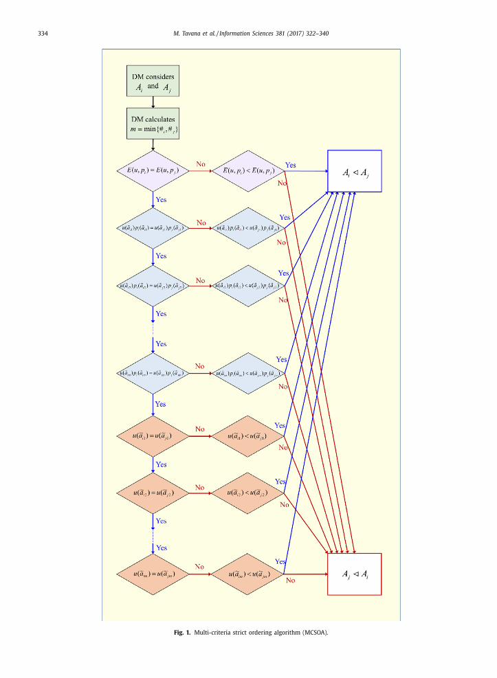
able to compare them with respect to ≺� U . Thus, Definition 10 and Theorem 1 yield a multi-criteria strict ordering algorithm ,

consisting of three main steps through which D is guaranteed a final strict ranking of the alternatives. The multi-criteria

strict ordering algorithm (MCSOA) for two alternatives A i and A j is outlined below.

Multi-criteria Strict Ordering Algorithm (MCSOA)

Step 1. D checks whether or not A i and A j are comparable in expected utility terms.

Yes: D ranks the two alternatives.

No: D moves to the next step.

Step 2. D checks whether or not A i and A j are L-comparable.

Yes: D ranks the two alternatives.

No: D moves to the next step.

Step 3. A i and A j are surely U-comparable: D ranks the two alternatives.

Fig. 1 provides a graphical representation of the above MCSOA inclusive of all the functions and the calculations involved

in each step.

Example 6. Suppose that D must rank six alternatives A 1 , …, A 6 offered by S 1 , …, S 6 , respectively. Suppose that a , a ’, b ,

b ’, c , c ’, d , d ’, e , f , g , h , h ’, h ”, k ∈ G are the alternatives that D uses to form the perceived possibility sets and that he

assigns the following utility values to these alternatives:

U(a ) = U(a ′ ) = 24 , U(b) = U(b ′ ) = 18 , U(c) = U(c ′ ) = 16 , U(d) = U(d ′ ) = 12 ,

U(e ) = 10 , U( f ) = 8 , U(g) = 6 , U(h ) = U(h

′ ) = U(h

′′ ) = 4 , U(k ) = 2 .

Then,

˜ a =

˜ a ′ , ˜ b =

˜ b ′ , ˜ c =

˜ c ′ , ˜ d =

˜ d ′ , ˜ h =

˜ h

′ =

˜ h

′′

and

u ( a ) = 24 , u ( b ) = 18 , u ( c ) = 16 , u ( d ) = 12 , u ( e ) = 10 , u ( f ) = 8 ,

u ( g ) = 6 , u ( h ) = 4 , u ( k ) = 2 .

Let the perceived possibility sets and the subjective beliefs of D be defined as in Table 6.

Step 1. Check E-comparability

Calculate the perception-based expected utilities:

E(u, p 1 ) = E(u, p 2 ) = E(u, p 3 ) = E(u, p 5 ) = 10

E(u, p 4 ) = E(u, p 6 ) = 13

Thus,

• A 4 and A 6 are both better than A 1 , A 2 , A 3 and A 5 in expected utility terms. • A 4 and A 6 are equally ranked. • A 1 , A 2 , A 3 and A 5 are equally ranked.

334 M. Tavana et al. / Information Sciences 381 (2017) 322–340

Fig. 1. Multi-criteria strict ordering algorithm (MCSOA).

M. Tavana et al. / Information Sciences 381 (2017) 322–340 335

Step 2. Check L-comparability

(2.1) Consider A 4 and A 6 . Both �4 and �6 have three elements.

Compute:

� L ( �4 | min { # 4 , # 6 } ) =

� L ( �4 | 3) =

(24 · 1

3 , 18 · 1

6 , 4 · 1

2

)= (8 , 3 , 2)

� L ( �6 | min { # 4 , # 6 } ) =

� L ( �6 | 3) =

(16 · 1

2 , 12 · 1

4 , 8 · 1

4

)= (8 , 3 , 2) .

Since they coincide, A 4 and A 6 are not L-comparable and are still equally ranked.

(2.2) Consider A 1 and A 2 . The perceived possibility sets �1 and �2 have one and two elements, respectively.

Compute:

� L ( �1 | min { # 1 , # 2 } ) =

� L ( �1 | 1) = ( 10 · 1 ) = (10)

� L ( �2 | min { # 1 , # 2 } ) =

� L ( �2 | 1) =

(18 · 1

2

)= (9) .

Since (9) < Lex (10), A 2 ≺� L A 1 . Hence, A 2 � A 1 .

(2.3) Consider A 2 and A 3 . The perceived possibility sets �2 and �3 have two and three elements, respectively.

Compute:

� L ( �2 | min { # 2 , # 3 } ) =

� L ( �2 | 2) =

(18 · 1

2 , 2 · 1

2

)= (9 , 1)

� L ( �3 | min { # 2 , # 3 } ) =

� L ( �3 | 2) =

(24 · 1

6 , 12 · 1

3

)= (4 , 4) .

Since (4, 4) < Lex (9, 1), A 3 ≺� L A 2 . Hence, A 3 � A 2 .

(2.4) Consider A 3 and A 5 . The perceived possibility sets �3 and �5 have three and four elements, respectively.

Compute:

� L ( �3 | min { # 3 , # 5 } ) =

� L ( �3 | 3) =

(24 · 1

6 , 12 · 1

3 , 4 · 1

2

)= (4 , 4 , 2)

� L ( �5 | min { # 3 , # 5 } ) =

� L ( �5 | 3) =

(16 · 1

4 , 12 · 1

3 , 6 · 1

6

)= (4 , 4 , 1) .

Since (4, 4, 1) < Lex (4, 4, 2), A 5 ≺� L A 3 . Hence, A 5 � A 3 .

Step 3. Check U-comparability

Consider A 4 and A 6 . Both �4 and �6 have three elements.

Compute:

� U ( �4 | min { # 4 , # 6 } ) =

� U ( �4 | 3) = ( 24 , 18 , 4 )

� U ( �6 | min { # 4 , # 6 } ) =

� U ( �6 | 3) = ( 16 , 12 , 8 ) .

Since (16, 12, 8) < Lex (24, 18, 4), A 6 ≺� U A 4 . Hence, A 6 � A 4 .

Final ranking (from the highest to the lowest): A 4 � A 6 � A 1 � A 2 � A 3 � A 5 .

The ranking scenario described in Example 6 provides the required intuition regarding the selection process defined by

the proposed MCSOA. In this regard, the evaluation of the information contained in online reviews, such as those available in

Amazon, Yelp and TripAdvisor, constitutes a natural environment to which the proposed algorithm can be directly applied.

We focus on the last website to describe an immediate application of the algorithm to a real-life setting, with the other

websites leading to very similar decision environments.

DMs accessing the TripAdvisor website to gather information about the hotels available within a given city have access

to reviews of multiple alternatives provided by different ISs. In addition to the linguistic descriptions, the rating summary

of the alternatives includes numerical evaluations of the following categories: location, sleep quality, rooms, service, value

and cleanliness. Thus, each one of the characteristics defining a given alternative has both a numerical value assigned by

the reviewer together with an extended linguistic description.

DMs are also endowed with a classification of the reviewers so as to discriminate among the considerable amount of

reports available per alternative. Reviewers are ranked using several predefined categories such as their level of contribution,

determined, among other variables, by their number of reviews. They are also assigned different distinctive badges ranging

from helpful votes to expertise.

Given the large amount of reviews providing the same numerical evaluation of each alternative, we could assume that

the DMs focus on one of them and use a description per alternative to generate the corresponding rankings. This behavior

is in line with the requirements allowing for the implementation of the MCSOA described in the paper.

The selection process of reviewers should be determined by the multiple reviews to which the DMs have access. That

is, the DMs can observe the linguistic and numerical evaluations provided by a given reviewer for different alternatives and

use them to construct a reliability index for the reviewer. We will analyze this possibility in Section 8 , when defining the

integration of reliability indexes within the current algorithm.

336 M. Tavana et al. / Information Sciences 381 (2017) 322–340

6. Matrix representation of the algorithm and its integration within the AHP framework

The proposed MCSOA allows for a matrix representation that can be useful from a more practical and computational

point of view, especially when there is a large number of alternatives to rank.

For every i ∈ {1, …, n }, consider the following row vector of dimension 2 max { # j : j = 1 , . . . , n } + 2 : (A i | E(u, p i ) | u ( a i 1 ) p i ( a i 1 ) · · · u ( a i # i ) p i ( a i # i ) ∗ · · · ∗ | u ( a i 1 ) · · · u ( a i # i ) ∗ · · · ∗

)The symbol ∗, in the third and fourth block, means “D does not calculate the next value”. Indeed, D cannot calculate

the element after u ( a i # i ) p i ( a i # i ) or after u ( a i # i ) since ˜ a i # i is the last element in � i . The symbol ∗ must appear max { # j : j =1 , . . . , n } − # i times in each block.

The row vector displays the perception-based expected utility that D assigns to A i followed by the tuple � L ( �i ) and the

tuple � U ( �i ) , that is, all the elements that the DM must use to compare the i th alternative A i with respect to the linear order

� .

The matrix composed by all the row vectors obtained as above facilitates the comparisons among all the alternatives. The

matrix has dimension n × (2( max { # j : j = 1 , . . . , n } + 1)) and displays the three steps of the ordering algorithm defined by

� explicitly and simultaneously; each step corresponds to one of the three blocks forming the matrix.

Up to a reordering of the rows, the first column of the matrix can be used to represent the strict ranking of the alterna-

tives from the highest to the lowest ranked one.

Example 7. The matrix representation of the situation described in Example 5 (see also Table 5 ) is the following: ⎛

⎝

A 1

A 2

A 3

∣∣∣∣∣∣10

10

10

∣∣∣∣∣∣10 · 1 0 0

18 · 1 2

2 · 1 2

0

24 · 1 6

12 · 1 3

4 · 1 2

∣∣∣∣∣∣10 0 0

18 2 0

24 12 4

⎞

⎠

In this case, the order of the row already corresponds to the strict ranking (from the highest to the lowest) of the

alternatives, that is A 1 � A 2 � A 3 .

Example 8. The matrix representation of the situation described in Example 6 (see also Table 6 ) is the following: ⎛

⎜ ⎜ ⎜ ⎜ ⎜ ⎜ ⎝

A 1

A 2

A 3

A 4

A 5

A 6

∣∣∣∣∣∣∣∣∣∣∣∣

10

10

10

13

10

13

∣∣∣∣∣∣∣∣∣∣∣∣

10 · 1 ∗ ∗ ∗18 · 1

2 2 · 1

2 ∗ ∗

24 · 1 6

12 · 1 3

4 · 1 2

∗24 · 1

3 18 · 1

6 4 · 1

2 ∗

16 · 1 4

12 · 1 3

6 · 1 6

4 · 1 4

16 · 1 2

12 · 1 4

8 · 1 4

∗

∣∣∣∣∣∣∣∣∣∣∣∣

10 ∗ ∗ ∗18 2 ∗ ∗24 12 4 ∗24 18 4 ∗16 12 6 4

16 12 8 ∗

⎞

⎟ ⎟ ⎟ ⎟ ⎟ ⎟ ⎠

By the proposed MCSOA, we have A 4 � A 6 � A 1 � A 2 � A 3 � A 5 . Thus, we can rearrange the rows as follows: ⎛

⎜ ⎜ ⎜ ⎜ ⎜ ⎜ ⎝

A 4

A 6

A 1

A 2

A 3

A 5

∣∣∣∣∣∣∣∣∣∣∣∣

13

13

10

10

10

10

∣∣∣∣∣∣∣∣∣∣∣∣

24 · 1 3

18 · 1 6

4 · 1 2

∗16 · 1

2 12 · 1

4 8 · 1

4 ∗

10 · 1 ∗ ∗ ∗18 · 1

2 2 · 1

2 ∗ ∗

24 · 1 6

12 · 1 3

4 · 1 2

∗16 · 1

4 12 · 1

3 6 · 1

6 4 · 1

4

∣∣∣∣∣∣∣∣∣∣∣∣

24 18 4 ∗16 12 8 ∗10 ∗ ∗ ∗18 2 ∗ ∗24 12 4 ∗16 12 6 4

⎞

⎟ ⎟ ⎟ ⎟ ⎟ ⎟ ⎠

The categorized structure of the MCSOA described through its matrix form provides the required intuition regarding one

of its main potential extensions, namely, its capacity to be integrated within the AHP framework. In particular, the decision

algorithm has been designed to highlight the recognized though seemingly forgotten fact that DMs must actually construct

their expected utility functions. This fact is acknowledged in the standard microeconomic textbooks [32] , but only explicitly

analyzed whenever violations of the expected utility axioms are observed [40] .

In this regard, the experiments designed by psychologists and economists present the DMs with a given set of lotteries

among which to choose. The set of expected payoffs is specifically designed to study a given feature of the evaluation and

choice process. Therefore, it is directly given to the DMs, while a range of potential utilities is considered and tested when

eliciting their preferences. As a consequence, violations of the expected utility axioms are generally dealt with through

adjustments of the subjective probabilities defined by the DMs [39,55] .

We have followed a completely different approach and required the DMs to build their whole evaluation and decision

environment, ranging from the set of potential categories to which the linguistically described alternatives may belong to

the subjective probabilities assigned to the correct interpretation of the descriptions received. These requirements involve

subjective evaluation and decision problems that the DMs must resolve outside the controlled experimental environments

presented in the literature.

M. Tavana et al. / Information Sciences 381 (2017) 322–340 337

Note that, as a matter of fact, the DMs must define three subjective rankings determined by three different orders before

making a choice using their expected utilities. The literature generally considers the ranking based on these latter evalua-

tions, though nothing prevents DMs from referring to any of the other two rankings whenever they cannot make a decision

based on their subjective expected utilities.

It should be highlighted that the subjective utility and probability functions defined by the DMs provide ordinal evalua-

tions used to generate the corresponding rankings [14] . The ordinal property of the utility functions allows for the type of

pairwise comparisons across alternatives required within the AHP setting. Note that the resulting decision framework is free

of the scaling problems exhibited by expected value computations, while allowing DMs to subjectively define the impor-

tance assigned to the different rankings [22,42] . That is, the corresponding AHP weights can be defined by the DMs based

on the relative importance assigned to each different ranking.

Finally, note that the disaggregated decision structure defining the MCSOA provides a simple representation of the po-

tential choices that could be made by the DMs. Considering simpler evaluation procedures, other than those based on ag-

gregated expected utilities, allows DMs to deal with their limited information assimilation and processing capacities. The

resulting choices observed could therefore be based on the ranking they feel more comfortable implementing, whose rela-

tive importance could be tested empirically.

7. L-compatibility and U-compatibility for uncertainty averse DMs

The MCSOA proposed in this paper is based on the MaxMax approach, which generally reflects the behavior of DMs

who are not particularly concerned with uncertainty-related problems. Both notions of L-compatibility and U-compatibility

have been introduced exploiting such an approach, that is, assuming that the DM makes pairwise comparisons between the

perceived alternatives starting with the most preferred ones.

However, alternative approaches, such as the MaxMin approach, can also be implemented in our MCSOA. The MaxMin

approach is usually followed to model DMs characterized by an uncertainty averse behavior [25] .

For the sake of completeness, we shortly outline how the tuples L ( �i ) and U ( �i ) , for i = 1, …, n , have to be modified in

this alternative approach. The corresponding L-compatibility and U-compatibility relations are defined as in Definitions 6 –9.

MaxMin approach: The tuples L ( �i ) and U ( �i ) , for i = 1, …, n , and their ε-restrictions are replaced by the following.

� L ( �i ) M axM in = (u ( a i # i ) p i ( a i # i ) , . . . , u ( a i 2 ) p i ( a i 2 ) , u ( a i 1 ) p i ( a i 1 )) . (13)

� L ( �i | ε) M axM in =

{(u ( a i # i ) p i ( a i # i ) , u ( a i, # i −1 ) p i ( a i, # i −1 ) , . . . , u ( a i, # i −ε+1 ) p i ( a i, # i −ε+1 )) i f ε < # i � L ( �i ) M axM in i f ε ≥ # i

(14)

� U ( �i ) M axM in = (u ( a i # i ) , . . . , u ( a i 2 ) , u ( a i 1 )) . (15)

� U ( �i | ε) M axM in =

{(u ( a i # i ) , u ( a i, # i −1 ) , . . . , u ( a i, # i −ε+1 )) i f ε < # i � U ( �i ) M axM in i f ε ≥ # i

(16)

8. Strict ordering algorithm with reliability indexes

The MCSOA introduced in the paper is sufficiently flexible so as to incorporate the effect of online recommendation

agents into its tie-breaking structure [26,30,57] . Recommendation agents are software agents who use the purchasing his-

tory of consumers to elicit their preferences and suggest potential products for future purchase. Note that evaluating the

substantial amount of consumer reviews available online has similar analytical implications [58] . In both cases, the possibil-

ity of strategic reporting [15,38] leads to credibility and trust problems that must be addressed by the DM before making a

choice [23] .

That is, despite the verifiability of the information provided by the ISs, lexicographic information acquisition processes

and choices can be strategically induced on the DM [15,16] . Given the lexicographic choice rule defined by our algorithm

and the fact that the linguistic reports provided by the ISs are subjectively elaborated and imprecise, the problem of lexi-

cographically manipulable choice must be considered by the DM. This section describes a selection mechanism that softens

the effect of manipulation on the side of the DM and implements it within the ranking algorithm introduced in the paper.

Following Tavana et al. [53,54] , we observe that the characteristics listed in a given description, the order in which they

are displayed and their values depend on the viewpoint of the IS. That is, the IS decides the relative importance of the

characteristics and provides a subjective evaluation of each one of them when proposing an alternative to the DM.

Clearly, the DM aims at choosing the best alternative from his own viewpoint. Thus, a key role in the choice process is

played by the way the DM interprets the descriptions provided by the ISs. This interpretation is based on the perception

that the DM has of each possible alternative and, in particular, of its characteristics. Tavana et al. [54] designed a composite

index to weight the perception-based expected utility of the DM and rank the available alternatives.

338 M. Tavana et al. / Information Sciences 381 (2017) 322–340

I

I

The basic framework of Tavana et al. [54] is similar to ours: a DM must rank n alternatives, each one of them composed

by � characteristics described by an IS. The authors endow each IS with a linear order on the set � of all possible charac-

teristics composing any alternative. The DM is either allowed to check all the information provided by each IS or constrained

to check only a part of this information, acquiring the same amount of information from each IS.

However, differently from the current setting, the ranking criterion proposed by Tavana et al. [54] is based on the key

idea that the order in which the information is provided does not only differ across ISs but also affects the way the DM

ranks the alternatives. That is, the authors construct an ordinal raking criterion determined by the level of coordination

existing between the order assigned by the DM on the set of characteristics and those assigned by the different ISs.

The “Ordinal Reliability Ranking” criterion suggested by Tavana et al. [54] , can be summarized as follows:

I. D checks the first J ∈ {1,…, | �|} pieces of information provided by each S i .

II. D defines a “relative coordination” index and a “relative synchronicity” index for each S i that are combined into a com-

posite reliability index I ( S i ) ∈ [0, 1].

II. D calculates the value of the composite reliability index I ( S i ) ∈ [0, 1] for each S i .

V. D calculates the weighted perception-based expected utility:

wE(u, p i ) = I( S i ) · E(u, p i ) = I( S i ) ·∑

A ∈ �i (J)

u (A ) · p i (A )

V. D ranks the values wE ( u , p 1 ),…, wE ( u , p n ) and, hence, the corresponding alternatives, from the highest to the lowest one.

This ranking criterion has the limitation that two alternatives can be ranked equally. Indeed, it could be the case that

wE ( u , p i ) = wE ( u , p j ), with i � = j . This limitation can be removed by applying a variant of our MCSOA.

It should be noted that in Tavana et al. [54] D is endowed with a strict preference relation. As a consequence, the set G

of all existing alternatives coincides with the set �of all categories, the utility function U coincides with the induced utility

u and the set � i ( J ) is composed by alternatives instead of categories.

Consider the following weighted version of Definitions 4 , 6 and 8.

Definition 11. We denote by ≺wE , ≺w

� L and ≺w

� U the binary relations on � defined as follows:

∀ A i , A j ∈ �, A i ≺wE A j de f ←→ wE(u, p i ) < wE(u, p j ) , (17)

∀ A i , A j ∈ �, A i ≺w

� L A j

de f ←→ w

� L ( �i | m i j ) < Lex w

� L ( � j | m i j ) , (18)

∀ A i , A j ∈ �, A i ≺w

� U A j

de f ←→ w

� U ( �i | m i j ) < Lex w

� U ( �i | m i j ) , (19)

where

m i j = min { # i , # j } wE(u, p i ) = I( S i ) · E(u, p i ) wE(u, p j ) = I( S j ) · E(u, p j ) w

� L ( �i | m i j ) = (I( S i ) u ( a i 1 ) p i ( a i 1 ) , I( S i ) u ( a i 2 ) p i ( a i 2 ) , . . . , I( S i ) u ( a i m i j

) p i ( a i m i j ))

w

� L ( � j | m i j ) = (I( S j ) u ( a j1 ) p j ( a j1 ) , I( S j ) u ( a j2 ) p j ( a j2 ) , . . . , I( S j ) u ( a j m i j

) p j ( a j m i j ))

w

� U ( �i | m i j ) = (I( S i ) u ( a i 1 ) , I( S i ) u ( a i 2 ) , . . . , I( S i ) u ( a i m i j

))

w

� U ( � j | m i j ) = (I( S j ) u ( a j1 ) , I( S j ) u ( a j2 ) , . . . , I( S j ) u ( a j m i j

))

. (20)

Then, we can create a strict ranking of the alternatives using the algorithm induced by the following linear order.

Definition 12. We denote by � w

the binary relation on � defined as follows. For every A i , A j ∈ �,

A i � w

A j de f ←→

⎧ ⎪ ⎪ ⎪ ⎪ ⎪ ⎪ ⎪ ⎪ ⎪ ⎪ ⎨

⎪ ⎪ ⎪ ⎪ ⎪ ⎪ ⎪ ⎪ ⎪ ⎪ ⎩

A i ≺wE A j

or [( A i ⊀wE A j ) ∧ ( A j ⊀wE A i )

]∧ ( A i ≺w

� L A j )

or [( A i ⊀wE A j ) ∧ ( A j ⊀wE A i )

]∧

[( A i ⊀w

� L A j ) ∧ ( A j ⊀w

� L A i )

]∧ ( A i ≺w

� U A j )

or [( A i ⊀wE A j ) ∧ ( A j ⊀wE A i )

]∧

[( A i ⊀w

� L A j ) ∧ ( A j ⊀w

� L A i )

]∧ [

( A i ⊀w

� U A j ) ∧ ( A j ⊀w

� U A i )

]∧ ( A i ≺�

U A j )

(21)

Theorem 2. The binary relation � w

is a linear order on �.

The proof that � w

is a linear order ( Theorem 2 ) is analogous to that of Theorem 1 by considering the way the tuples

w

� L ( �i | min { # i , # j } ) and w

� U ( �i | min { # i , # j } ) are defined.

M. Tavana et al. / Information Sciences 381 (2017) 322–340 339

Building on the TripAdvisor example described in Section 5 , we can see how weighting the expected utilities by the

reliability assigned to each IS generates an additional level of potential indecisiveness among DMs. As a result, two dif-

ferent alternatives in �, which are now also weighted by the reliability of the reviewer, are not necessarily wE , w L or

w U -comparable for D .

Clearly, a strict ranking could be guaranteed by implementing the binary relation � w

introduced in Definition 12 . How-

ever, the strategic reporting capacity of reviewers may lead the DMs to aggregate the evaluations of several reviewers on a

given alternative, which would give place to different rankings depending on the reliability of the reviewers considered. We

return to this potential extension in the conclusion section below.

9. Conclusion

The current paper has introduced a novel multi-criteria algorithm that generates a strict order over any set of available

alternatives when the DMs are unable to decide among them. We have assumed that the DMs are endowed with limited

information processing capacities while receiving linguistic descriptions from different ISs regarding the characteristics of

several alternatives. We have illustrated how the algorithm can be designed to account for differences in the attitude to-

wards uncertainty of the DMs and for the strategic manipulation of the information provided by the ISs.

Given the capacity of the proposed algorithm to incorporate reliability indexes, an immediate extension of the current

paper would consist of implementing these tie-breaking algorithms within a setting where ISs and DMs interact strategi-

cally while acknowledging the imprecision existing both in the linguistic reports provided by the ISs and the subjective

interpretation and evaluations of the DM.

Acknowledgment

The authors would like to thank the anonymous reviewers and the editor for their insightful comments and suggestion.

References

[1] G.A. Akerlof , R.J. Shiller , Phishing for Phools: The Economics of Manipulation and Deception, University Press, Princeton, 2015 .

[2] R.A. Aliev , W. Pedrycz , O.H. Huseynov , Decision theory with imprecise probabilities, Int. J. Inf. Technol. Decis. Mak. 11 (2) (2012) 271–306 . [3] R.A. Aliev , W. Pedrycz , O.H. Huseynov , Behavioral decision making with combined states under imperfect information, Int. J. Inf. Technol. Decis. Mak.

12 (3) (2013) 619–645 . [4] C.J. Anderson , The psychology of doing nothing: forms of decision avoidance result from reason and emotion, Psychol. Bull. 129 (2013) 139–167 .

[5] K. Atanassov , Intuitionistic fuzzy sets, Fuzzy Sets Syst. 20 (1986) 87–96 . [6] S. Bae , T. Lee , Gender differences in consumers’ perception of online consumer reviews, Electron. Commer. Res. 11 (2011) 201–214 .

[7] D.M. Bartels , E.J. Johnson , Connecting cognition and consumer choice, Cognition 135 (2015) 47–51 . [8] J. Beattie , S. Barlas , Predicting perceived differences in tradeoff difficulty, in: E.U. Weber, J. Baron, G. Loomes (Eds.), Conflict and Tradeoffs in Decision

Making, Eds., Cambridge University Press, 2001, pp. 25–64 .

[9] J.R. Bettman , An Information Processing Theory of Consumer Choice, Addison-Wesley, 1979 . [10] T.F. Bewley , Knightian decision theory: Part I, Decis. Econ. Financ. 25 (2002) 79–110 .

[11] N. Chater , Can cognitive science create a cognitive economics, Cognition 135 (2015) 52–55 . [12] R. Hertwig , G. Barron , E.U. Weber , I. Erev , Decisions from experience and the effect of rare events in risky choice, Psychol. Sci. 15 (2004) 534–539 .

[13] E. Danan , Randomization vs selection: How to choose in the absence of preference, Manag. Sci. 56 (2010) 503–518 . [14] D. Di Caprio , F.J. Santos Arteaga , Cardinal versus ordinal criteria in choice under risk with disconnected utility ranges, J. Math. Econ. 47 (2011) 588–594 .

[15] D. Di Caprio , F.J. Santos Arteaga , Strategic diffusion of information and preference manipulation, Int. J. Strateg. Dec. Sci. 2 (2011) 1–19 .

[16] D. Di Caprio , F.J. Santos Arteaga , Lexicographic preferences induced in asymmetric information environments, Commun. Math. Appl. 1 (2010) 1–14 . [17] D.L. Diab , M.A. Gillespie , S. Highhouse , Are maximizers really unhappy? The measurement of maximizing tendency, Judgm. Decis. Mak. 3 (2008)

364–370 . [18] K. Eliaz , E.A. Ok , Indifference or indecisiveness? Choice theoretic foundations of incomplete preferences, Games Econ. Behav. 56 (2006) 61–86 .

[19] R. Engelking , General Topology, Heldermann Verlag, Berlin, 1989 . [20] J.R. Ferrari , J.F. Dovidio , Behavioral information search by indecisives, Personal. Individ. Differ. 30 (2001) 1113–1123 .

[21] P.C. Fishburn , Utility Theory and Decision Making, John Wiley & Sons, 1970 .

[22] E.H. Forman , AHP is intended for more than expected value calculations, Decis. Sci. 21 (1990) 670–672 . [23] F. Fouss , Y. Achbany , M. Saerens , A probabilistic reputation model based on transaction ratings, Inf. Sci. 180 (2010) 2095–2123 .

[24] G. Gigerenzer , R. Selten , Bounded Rationality: The Adaptive Toolbox, The MIT Press, 2002 . [25] I. Gilboa , D. Schmeidler , Maxmin expected utility with non-unique prior, J. Math. Econ. 18 (1989) 141–153 .

[26] R.E. Hostler , V.Y. Yoon , Z. Guo , T. Guimaraes , G. Forgionne , Assessing the impact of recommender agents on on-line consumer unplanned purchasebehavior, Inf. Manag. 48 (2011) 336–343 .

[27] S. Huang , Z. Niu , Y. Shi E. Métais, F. Meziane, M. Saraee, V. Sugumaran, S. Vadera (Eds.), Product features categorization using constrained spectral

clustering, Natural Language Processing and Information Systems (2013) 285–290 . [28] M.D. Johnson , A. Herrmann , F. Huber , The evolution of loyalty intention, J. Market. 70 (2006) 122–132 .

[29] D. Kahneman , A. Tversky , Choice, Values, and Frames, Cambridge University Press, 20 0 0 . [30] Y.M. Li , C.L. Chou , L.F. Lin , A social recommender mechanism for location-based group commerce, Inf. Sci. 274 (2014) 125–142 .

[31] M.F. Luce , Choosing to avoid: coping with negatively emotion laden consumer decisions, J. Consum. Res. 24 (1998) 409–433 . [32] A. Mas-Colell , M.D. Whinston , J.R. Green , Microeconomic Theory, Oxford University Press, 1995 .

[33] J.R. Munkres , Topology, Prentice Hall, 20 0 0 .

[34] M.J. Osborne , A. Rubinstein , A Course in Game Theory, The MIT Press, 1994 . [35] A.L. Patalano , Z. LeClair , The influence of group decision making on indecisiveness-related decisional confidence, Judgm. Decis. Mak. 6 (2011) 163–175 .

[36] W.J. Payne , J.R. Bettman , E.J. Johnson , The Adaptive Decision Maker, Cambridge University Press, 1993 . [37] W. Pedrycz , F. Gomide , An Introduction to Fuzzy Sets: Analysis and Design, The MIT Press, 1998 .

[38] R.A. Peterson , M.C. Merino , Consumer information search behavior and the internet, Psychol. Market. 20 (2003) 99–121 . [39] J. Quiggin , Generalized Expected Utility Theory. The Rank-Dependent Model, Kluwer Academic Publishers, 1993 .

340 M. Tavana et al. / Information Sciences 381 (2017) 322–340

[40] J. Rieskamp , J. Busemeyer , B. Mellers , Extending the bounds of rationality: Evidence and theories of preferential choice, J. Econ. Lit. XLIV (2006)631–661 .

[41] E. Rosch , Cognitive representation of semantic categories, J. Exp. Psychol. Gen. 104 (1975) 192–233 . [42] T.L. Saaty , A note on the AHP and expected value theory, Socio-Econ. Plan. Sci. 20 (1986) 397–398 .

[43] T.L. Saaty , The Analytic Hierarchy Process, McGraw-Hill, 1980 . [44] A .A . Salo , R.P. Hämäläinen , On the measurement of preferences in the analytic hierarchy process, J. Multi-Criteria Decis. Anal. 6 (1997) 309–319 .

[45] S. Samiee , Shimp T.A. , S. Sharma , Brand origin recognition accuracy: Its antecedents and consumers’ cognitive limitations, J. Int. Bus. Stud. 36 (2005)

379–397 . [46] B. Schwartz , Paradox of Choice, Harper Perennial, 2004 .

[47] S.M. Shugan , The cost of thinking, J. Consum. Res. 7 (1980) 99–111 . [48] H.A. Simon , A behavioral model of rational, Q. J. Econ. 79 (1955) 99–118 .

[49] H.A. Simon , Administrative Behaviour, Free Press, 1997 . [50] N. Stewart , N. Chater , G.D. Brown , Decision by sampling, Cogn. Psychol. 53 (2006) 1–26 .

[51] M. Sujan , A.M. Tybout , Applications and extensions of categorization research in consumer behavior, in: M.J. Houston (Ed.), Advances in ConsumerResearch, 15, Ed., Association for Consumer Research, 1988, pp. 50–54 .

[52] E. Szmidt , Distances and Similarities in Intuitionistic Fuzzy Sets, Springer International Publishing, 2014 .

[53] M. Tavana , D. Di Caprio , F.J. Santos-Arteaga , A bilateral exchange model: the paradox of quantifying the linguistic values of qualitative characteristics,Inf. Sci. 296 (2015) 201–218 .

[54] M. Tavana , D. Di Caprio , F.J. Santos-Arteaga , An ordinal ranking criterion for the subjective evaluation of alternatives and exchange reliability, Inf. Sci.317 (2015) 295–314 .

[55] A. Tversky , D. Kahneman , Advances in prospect theory: Cumulative representation of uncertainty, J. Risk Uncertain. 5 (1992) 297–323 . [56] A. Tversky , E. Shafir , Choice under conflict: the dynamics of deferred decision, Psychol. Sci. 6 (1992) 358–361 .

[57] B. Xiao , I. Benbasat , E-commerce product recommendation agents: use, characteristics, and impact, MIS Q. 31 (2007) 137–209 .

[58] Z. Yan , M. Xing , D. Zhang , B. Ma , EXPRS: An extended page rank method for product feature extraction from online consumer reviews, Inf. Manag. 52(7) (2015) 850–858 .

[59] L. Zadeh , The concept of a linguistic variable and its application to approximate reasoning-I, Inf. Sci. 8 (3) (1975) 199–249 .