Embed Size (px)
Citation preview
ARTICLE IN PRESS
0306-4379/$ - se
doi:10.1016/j.is.
�Correspondfax: +1267 295
E-mail addre
joglekar@lasall
(M.A. Redmon
URL: http:/
Information Systems 32 (2007) 773–792
www.elsevier.com/locate/infosys
An automated entity–relationship clustering algorithmfor conceptual database design
Madjid Tavanaa,�, Prafulla Joglekara, Michael A. Redmondb
aManagement Department, La Salle University, Philadelphia, PA 19141, USAbDepartment of Mathematics and Computer Science, La Salle University, Philadelphia, PA 19141, USA
Received 31 December 2005; received in revised form 6 July 2006; accepted 11 July 2006
Recommended by F. Carino Jr.
Abstract
Entity–relationship (ER) modeling is a widely accepted technique for conceptual database design. However, the
complexities inherent in large ER diagrams have restricted the effectiveness of their use in practice. It is often difficult for
end-users, or even for well-trained database engineers and designers, to fully understand and properly manage large ER
diagrams. Hence, to improve their understandability and manageability, large ER diagrams need to be decomposed into
smaller modules by clustering closely related entities and relationships. Previous researchers have proposed many manual
and semi-automatic approaches for such clustering. However, most of them call for intuitive and subjective judgment from
‘‘experts’’ at various stages of their implementation. We present a fully automated algorithm that eliminates the need for
subjective human judgment. In addition to improving their understandability and manageability, an automated algorithm
facilitates the re-clustering of ER diagrams as they undergo many changes during their design, development, and
maintenance phases.
The validation methodology used in this study considers a set of both objective and subjective criteria for comparison.
We adopted several concepts and metrics from machine-part clustering in cellular manufacturing (CM) while exploiting
some of the characteristics of ER diagrams that are different from typical CM situations. Our algorithm uses well
established criteria for good ER clustering solutions. These criteria were also validated by a group of expert database
engineers and designers at NASA. An objective assessment of sample problems shows that our algorithm produces
solutions with a higher degree of modularity and better goodness of fit compared with solutions produced by two
commonly used alternative algorithms. A subjective assessment of sample problems by our expert database engineers and
designers also found our solutions preferable to those produced by the two alternative algorithms.
r 2006 Elsevier B.V. All rights reserved.
Keywords: Computers; Databases; Information systems; Analysis and designs; Planning; Decision analysis
e front matter r 2006 Elsevier B.V. All rights reserved
2006.07.001
ing author. Tel.: +1215 951 1129;
2854.
sses: [email protected] (M. Tavana),
e.edu (P. Joglekar), [email protected]
d).
/lasalle.edu/�tavana.
1. Introduction
Entity–relationship (ER) modeling [1] is a popu-lar and effective methodology used to construct aconceptual data model. An ER diagram (ERD)is a detailed graphical representation of the data
.

ARTICLE IN PRESSM. Tavana et al. / Information Systems 32 (2007) 773–792774
requirements in an organization or business unit.ERDs enhance understanding of the system andimprove communication among database engineers,designers, and end-users.
Consider the following business scenario docu-mented during systems analysis for the developmentof an information system for a retailer of custom-made products:
A customer issues a purchase order to the vendor
(retailer) to buy a product. The purchase orderconsists of an order item. When the product isdelivered, the customer is given a receipt for theproduct. Because the customer has a line of credit,the actual payment is deferred until later. In thenext billing cycle, the vendor issues an invoice thatincludes an invoice item related to the order item
on the purchase order. Upon receiving the invoice,the customer makes sales payment against thereceipt of the product and the vendor receivesvendor payment for the invoice.
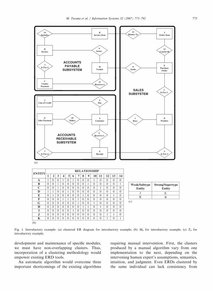
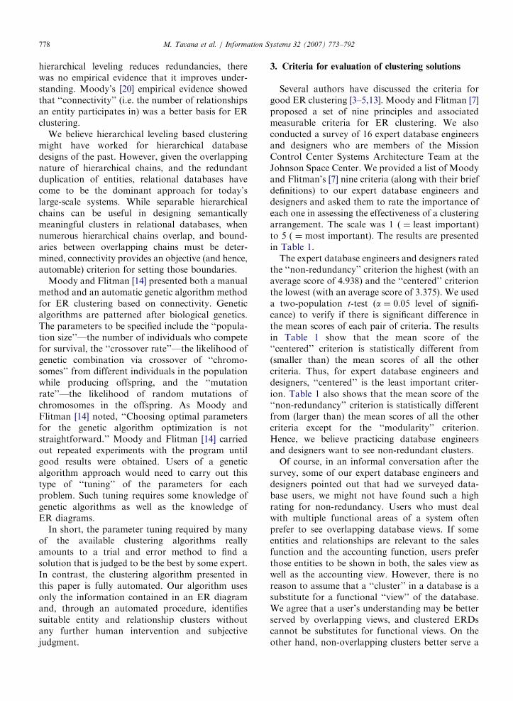
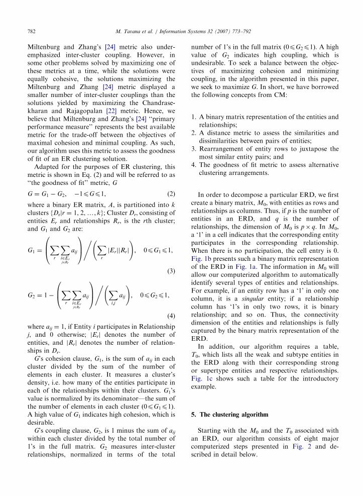
This scenario results in the identification of theentities and relationships presented in a clusteredERD presented in Fig. 1a. Entities are representedby rectangles, relationships by diamond-shapedboxes, and connecting lines show which entitiesparticipate in which relationship [1]. For example,the fact that a customer (Entity A) buys a product(Entity D) is represented by the ‘‘buy’’ relationship(Relationship 1). Knowledgeable end-users cancomprehend and validate the database designimplied by an ERD against actual business prac-tices. Once finalized, an ERD serves as the blueprintfor database implementation.
The ER model has become so common indatabase design that today a number of commercialER diagraming tools are available (e.g. ERWin byComputer Associates, EasyER by Visible Systems,Visio by Microsoft, and ER/1 by Embarcadero). ERtools differ somewhat in their terminology andnotation. However, the basic concepts are the sameand all ER tools represent data requirementsgraphically. Several tools generate the code neededfor the database schema, including the necessarytables, indexes, triggers, and stored procedures.Most ER tools support systems analysis anddatabase design, implementation, and maintenance.
Yet, today ER tools fall short of their truepotential. This is because ER diagrams are rarely assmall as the one presented in Fig. 1a. A typicalapplication data model consists of 95 entities and anaverage enterprise model consists of 536 entities [2].
Feldman and Miller [3] suggest that diagramsinvolving 30 or more entities exceed the limits ofeasy comprehension, and communications. Toimprove their understandability and manageability,large ER diagrams need to be decomposed intosmaller modules by clustering closely related entitiesand relationships.
The ERD in Fig. 1a is small enough tocomprehend without any decomposition. However,the three clusters (retailer’s ‘‘sales,’’ ‘‘accountsreceivable,’’ and ‘‘accounts payable’’ subsystems)identified by our algorithm illustrate some of theadvantages of decomposing ERDs. The literatureon clustering [3–6] has identified several advantagesof ERD decomposition. Clustered ER diagrams:
1.
Are easier to develop and maintain, since theyare more modular;2.
Are easier to document, since clusters are smallerand easier to understand;3.
Are easier to validate, since they provide betterorganization;4.
Can assist project management by allowingallocation of modular tasks to individuals orteams; and5.
Can assist identification of reusable subsystemsthat can be added, removed, or modifiedrelatively independently of one another.In spite of these advantages, today no ERdiagramming tool offers any clustering assistance.This is mainly because the available ER clusteringalgorithms call for intuitive and subjective judgmentfrom ‘‘experts’’ at various stages of their implemen-tation (see Section 2). ER tools support data modelconstruction, communication, and validation bystoring all the entities, relationships, relevantassumptions, and constraints in a repository. Usingthe repository, multiple conceptual and physical-level ERD ‘‘views’’ can be produced for specificpurposes such as end-user communication, databasedesign, and development by presenting only rele-vant portions of the larger design to specificaudiences. Users often prefer such views. As such,we do not want to suggest that clustered diagramswould replace functional views of a database.
However, sometimes even these views are toolarge for adequate comprehension. More impor-tantly, because specific entities and relationships areoften duplicated in several views, the ‘‘views’’ do notoffer some of the advantages of a clustered ERD.For example, in allocating responsibility for the
ARTICLE IN PRESS
CVendor
Payment
BInvoice
HVendor
EPurchase
Order
DProduct
ACustomer
FReceipt
GSales Payment
3Is For-2
9Issues
11Receives-2
8Sends
13Consist Of
2Is For-1
1Buys
4 Receives-1
5Is For-3
10Makes
7Is For-4
ILine of Credit
6Has
JOrder Item
12Relates To
KInvoice Item
14Includes
ACCOUNTSPAYABLE
SUBSYSTEM
SALESSUBSYSTEM
ACCOUNTSRECEIVABLESUBSYSTEM
(a)
RELATIONSHIPENTITY
1 2 3 4 5 6 7 8 9 10 11 12 13 14A 1 0 0 1 0 1 0 0 0 1 0 0 0 0B 0 0 1 0 0 0 0 0 1 0 0 0 0 1C 0 0 1 0 0 0 0 0 0 0 1 0 0 0D 1 1 0 0 1 0 0 0 0 0 0 0 0 0E 0 1 0 0 0 0 0 1 0 0 0 0 1 0F 0 0 0 1 1 0 1 0 0 0 0 0 0 0G 0 0 0 0 0 0 1 0 0 1 0 0 0 0H 0 0 0 0 0 0 0 1 1 0 1 0 0 0I 0 0 0 0 0 1 0 0 0 0 0 0 0 0J 0 0 0 0 0 0 0 0 0 0 0 1 1 0K 0 0 0 0 0 0 0 0 0 0 0 1 0 1
(b)
Weak/SubtypeEntity
Strong/SupertypeEntity
JK
(c)
EB
Fig. 1. Introductory example: (a) clustered ER diagram for introductory example; (b) M0 for introductory example; (c) T0 for
introductory example.
M. Tavana et al. / Information Systems 32 (2007) 773–792 775
development and maintenance of specific modules,we must have non-overlapping clusters. Thus,incorporation of a clustering methodology wouldempower existing ERD tools.
An automatic algorithm would overcome threeimportant shortcomings of the existing algorithms
requiring manual intervention. First, the clustersproduced by a manual algorithm vary from oneimplementation to the next, depending on theintervening human expert’s assumptions, semantics,intuition, and judgment. Even ERDs clustered bythe same individual can lack consistency from
ARTICLE IN PRESSM. Tavana et al. / Information Systems 32 (2007) 773–792776
one attempt to the next. In repeated trials, anautomatic algorithm will produce the same solutionfor a given problem and consistent solutions tosimilar problems.
Second, manual algorithms may work fine forsmall ERDs. However, for typical real-life (andlarge) ERDs, they are not likely to produce a goodsolution that seeks several clustering objectivessimultaneously. As Moody and Flitman [7] pointout, ‘‘Because of the enormous number of decom-positions that are possible in even small datamodels, it is clearly beyond human cognitivecapabilities to find an optimal solution. Accordingto the principle of bounded rationality, humans willonly explore a limited range of alternatives andconsider a subset of the decomposition objectives inorder to make the task cognitively manageable y’’
Third, manual algorithms take considerableamounts of time to implement. In today’s highlydynamic business environment with numerousmergers and acquisitions, existing business modelsbecome obsolete at an increasing pace. The abilityto rapidly change databases and their underlyingdata models to support the needs of changingbusiness models is high on the research agenda ofinformation systems researchers [8].
In spite of their limitations, manual methodsmight have produced satisfactory decompositions oftraditional transactional processing systems invol-ving static and localized databases. However, newapplications (from E-commerce to web-based deci-sion support systems, and from multimedia togeographic information systems) demand integrateddatabases with more entities, relationships, attri-butes, data elements, etc. [9,10]. The added seman-tics and complexity require that database engineersand designers revisit their conceptual data modelsperiodically in an attempt to expand or modify them[11,12]. Furthermore, in software engineering,emphasis has shifted from a rigid system design,where the software is available at the end of theprocess, to an incremental and modular designbased on iterative clustering refinements [10].Clearly, an automated clustering algorithm canmake iterative refinements considerably simplerand faster. According to Francalanci and Pernici[5], in legacy database re-engineering, automatedclustering is particularly useful due to the size of theexisting physical schema.
Hence, it is no surprise that recent work in ERclustering has aimed at automated algorithms[4,5,13,14]. Ideally, given the information obtained
by database engineers and designers during theconstruction of an ERD, an automated algorithmshould identify suitable entity and relationshipclusters without further human intervention. Un-fortunately, none of the above referenced worksmeets that ideal. In this paper, we present a fullyautomated ERD decomposition algorithm thatmeets this ideal.
Clustering problems arise in numerous domainsranging from weather forecasting, to epidemiology,cellular manufacturing (CM), linguistics, datamining, and economics. In different contexts,clustering takes different names such as typology,numerical taxonomy, and partitioning. Clusteringmethodologies originate in equally diverse disci-plines including neural networks, genetics, fuzzysets, matrix manipulation, mathematical program-ming, and multivariate analysis [15].
Traditionally, ERD clustering algorithms havefocused on the hierarchical levels of entities. Entitytypes are indeed an important consideration inERD clustering and our algorithm appropriatelyaccommodates different entity types. However,Moody and Flitman’s [16] recent experiment showsthat ‘‘connectivity’’ (or the number of relationshipsan entity participates in) is the more appropriatecriterion for ERD clustering than the hierarchicallevelling criterion. In CM, ‘‘connectivity,’’ or thenumber of machines (similar to relationships)processing a part (similar to entities) and thenumber of parts processed by a machine, has beenthe primary criterion for clustering. Hence, we haveadopted some of the CM concepts in designingour algorithm.
Furthermore, available ER clustering algo-rithms (with the exception of [17]) have focusedon clustering only the entities. However, asFrancalanci and Pernici [5] have noted, relation-ships play an important role in schema validation,schema reuse, and schema integration. We believethat the inclusion of relationships in ER clusteringprovides a more precise resource allocation planfor the development and maintenance of specificmodules. When a ‘‘boundary’’ relationship in-volves entities in two different modules, theresponsibility for coding and maintenance of thatrelationship must be assigned to one, and onlyone, of the two individuals (or teams) in charge ofthose two modules. Therefore, our algorithmclusters not only the entities but also the relation-ships. In CM, a manufacturing cell is formedonly when one identifies a group of machines
ARTICLE IN PRESSM. Tavana et al. / Information Systems 32 (2007) 773–792 777
as well as a ‘‘part family’’ that ‘‘the machinegroup’’ processes.
This paper is organized as follows. Section 2presents a review of prior work on ER clustering. InSection 3, we summarize the criteria for good ERclustering solutions. In Section 4, we outline therelevant concepts and metrics from CM that areused in our algorithm. In Section 5, we explain thelogic and details of our algorithm. Section 6discusses how the complexity of our algorithm iskept manageable and how it compares with a bruteforce approach to clustering. In Section 7, we assessthe effectiveness of our algorithm. In the availableliterature, we found only two examples of largeenough ER diagrams decomposed with alternativealgorithms. Hence, we compare our algorithm’ssolutions to those two problems with the solutionsby those algorithms. We show that our algorithmproduces better solutions than those obtained byother ERD clustering algorithms based on both, thecriteria established in Section 3 and the preferencesof a group of expert database engineers anddesigners at NASA. Our conclusions are summar-ized and directions for future research are outlinedin Section 8.
2. Prior work on ER clustering
In his earliest work on ER clustering, Martin [18]used ‘‘hierarchical leveling’’ to organize an ERDinto a set of hierarchies, each defined by a chainof one-to-many (parent–child) relationships. A‘‘root’’ entity with no many-to-one relationshipswas placed at the top of each hierarchy. Clusterswere formed with root entities as centers and theirdescendents as other elements in the cluster. Therequirement that main entities must have no many-to-one relationships was too inflexible. Whenhierarchical chains overlapped, human judgmentwas used to resolve boundaries. Two-level cluster-ing was considered an advantage of Martin’s [18]approach. At the second level, identified entityclusters were clustered into entity supergroups
based on the strength of association (frequency ofuse) between clusters. Feldman and Miller [3]changed Martin’s [18] second level clustering byfocusing on ‘‘subject areas’’ to group the entityclusters. Teorey et al.’s [6] method identified thesubject (or functional) areas first and then clusteredentities within a functional area by sequentiallygrouping weak entities with their dominant enti-ties, subtype entities with their supertypes, and
binary entities together, followed by tertiaryentities together. All of these methods dependedheavily on human judgment to resolve boundaries,to define strength of association, and/or to identifysuitable subject areas.
Huffman and Zoeller [13] were the first to attemptto automate ER clustering by developing an expertsystem to find the dominant entities based on a setof rules. However, Campbell et al. [19] suggestedthat the heuristic was too simplistic for complexcases and sometimes resulted in overlooked domi-nant entities. Francalanci and Pernici [5] presented asemi-automatic method in which each entity startedas its own cluster. Then the most closely linked pairof clusters was combined into one cluster. Thiscontinued until a predetermined number of clusterswere found. Unfortunately, determining the close-ness of a pair of clusters required a weightedaverage of human judgments on several dimensionsof similarities and dissimilarities among the entitiesand relationships in the two clusters. According toMoody and Flitman [7], this was an enormous taskand defeated the purpose of automation.
Akoka and Comyn-Wattiau’s [17] algorithmcomes closest to being fully automated. They definecloseness of entities by considering types of entitiesand relationships. The distance between a weakentity and its dominant entity is 1, between asupertype entity and its subtype entity is 10, betweentwo entities in an exclusive relationship is 100,between two entities involved in a binary relation-ship is 1000, and so on. This approach removesthe subjectivity of measurement. Once the distancesare established, Akoka and Comyn-Wattiau’s[17] algorithm can automatically find the ‘‘best’’solution for a prescribed number of clusters.A distinguishing feature of Akoka and Comyn-Wattiau’s [17] algorithm is that it clusters relation-ships as well as entities while other methods focuson clustering entities only. One shortcoming of thisalgorithm is that it provides no guidance for thenumber of clusters to be found. Furthermore, asMoody and Flitman [14] point out, it is difficult tojustify the weights assigned to each type of semanticdistance between entities.
While all of the foregoing algorithms can be seenas extensions of Martin’s [18] ‘‘hierarchical leveling’’approach, Moody [20] argued that hierarchicalleveling was inappropriate for ER clustering. Hefound no theoretical justification for it in theliterature. He argued that while there was strongevidence that grouping attributes based on
ARTICLE IN PRESSM. Tavana et al. / Information Systems 32 (2007) 773–792778
hierarchical leveling reduces redundancies, therewas no empirical evidence that it improves under-standing. Moody’s [20] empirical evidence showedthat ‘‘connectivity’’ (i.e. the number of relationshipsan entity participates in) was a better basis for ERclustering.
We believe hierarchical leveling based clusteringmight have worked for hierarchical databasedesigns of the past. However, given the overlappingnature of hierarchical chains, and the redundantduplication of entities, relational databases havecome to be the dominant approach for today’slarge-scale systems. While separable hierarchicalchains can be useful in designing semanticallymeaningful clusters in relational databases, whennumerous hierarchical chains overlap, and bound-aries between overlapping chains must be deter-mined, connectivity provides an objective (and hence,automable) criterion for setting those boundaries.
Moody and Flitman [14] presented both a manualmethod and an automatic genetic algorithm methodfor ER clustering based on connectivity. Geneticalgorithms are patterned after biological genetics.The parameters to be specified include the ‘‘popula-tion size’’—the number of individuals who competefor survival, the ‘‘crossover rate’’—the likelihood ofgenetic combination via crossover of ‘‘chromo-somes’’ from different individuals in the populationwhile producing offspring, and the ‘‘mutationrate’’—the likelihood of random mutations ofchromosomes in the offspring. As Moody andFlitman [14] noted, ‘‘Choosing optimal parametersfor the genetic algorithm optimization is notstraightforward.’’ Moody and Flitman [14] carriedout repeated experiments with the program untilgood results were obtained. Users of a geneticalgorithm approach would need to carry out thistype of ‘‘tuning’’ of the parameters for eachproblem. Such tuning requires some knowledge ofgenetic algorithms as well as the knowledge ofER diagrams.
In short, the parameter tuning required by manyof the available clustering algorithms reallyamounts to a trial and error method to find asolution that is judged to be the best by some expert.In contrast, the clustering algorithm presented inthis paper is fully automated. Our algorithm usesonly the information contained in an ER diagramand, through an automated procedure, identifiessuitable entity and relationship clusters withoutany further human intervention and subjectivejudgment.
3. Criteria for evaluation of clustering solutions
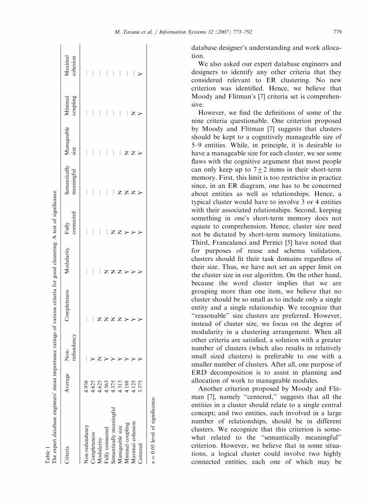
Several authors have discussed the criteria forgood ER clustering [3–5,13]. Moody and Flitman [7]proposed a set of nine principles and associatedmeasurable criteria for ER clustering. We alsoconducted a survey of 16 expert database engineersand designers who are members of the MissionControl Center Systems Architecture Team at theJohnson Space Center. We provided a list of Moodyand Flitman’s [7] nine criteria (along with their briefdefinitions) to our expert database engineers anddesigners and asked them to rate the importance ofeach one in assessing the effectiveness of a clusteringarrangement. The scale was 1 ( ¼ least important)to 5 ( ¼ most important). The results are presentedin Table 1.
The expert database engineers and designers ratedthe ‘‘non-redundancy’’ criterion the highest (with anaverage score of 4.938) and the ‘‘centered’’ criterionthe lowest (with an average score of 3.375). We useda two-population t-test (a ¼ 0:05 level of signifi-cance) to verify if there is significant difference inthe mean scores of each pair of criteria. The resultsin Table 1 show that the mean score of the‘‘centered’’ criterion is statistically different from(smaller than) the mean scores of all the othercriteria. Thus, for expert database engineers anddesigners, ‘‘centered’’ is the least important criter-ion. Table 1 also shows that the mean score of the‘‘non-redundancy’’ criterion is statistically differentfrom (larger than) the mean scores of all the othercriteria except for the ‘‘modularity’’ criterion.Hence, we believe practicing database engineersand designers want to see non-redundant clusters.
Of course, in an informal conversation after thesurvey, some of our expert database engineers anddesigners pointed out that had we surveyed data-base users, we might not have found such a highrating for non-redundancy. Users who must dealwith multiple functional areas of a system oftenprefer to see overlapping database views. If someentities and relationships are relevant to the salesfunction and the accounting function, users preferthose entities to be shown in both, the sales view aswell as the accounting view. However, there is noreason to assume that a ‘‘cluster’’ in a database is asubstitute for a functional ‘‘view’’ of the database.We agree that a user’s understanding may be betterserved by overlapping views, and clustered ERDscannot be substitutes for functional views. On theother hand, non-overlapping clusters better serve a
ARTICLE IN PRESS
Table
1
Theexpertdatabase
engineers’meanim
portance
ratingsofvariouscriteria
forgoodclustering:A
test
ofsignificance
Criteria
Average
Non-
redundancy
Completeness
Modularity
Fully
connected
Sem
antically
meaningful
Manageable
size
Minim
al
coupling
Maxim
al
cohesion
Non-redundancy
4.938
——
——
——
——
Completeness
4.625
Y—
——
——
——
Modularity
4.625
NN
——
——
——
Fullyconnected
4.563
YN
N—
——
——
Sem
anticallymeaningful
4.375
YN
NN
——
——
Manageable
size
4.313
YN
NN
N—
——
Minim
alcoupling
4.188
YY
YY
NN
——
Maxim
alcohesion
4.125
YY
YY
NN
N—
Centered
3.375
YY
YY
YY
YY
a¼
0.05level
ofsignificance.
M. Tavana et al. / Information Systems 32 (2007) 773–792 779
database designer’s understanding and work alloca-tion.
We also asked our expert database engineers anddesigners to identify any other criteria that theyconsidered relevant to ER clustering. No newcriterion was identified. Hence, we believe thatMoody and Flitman’s [7] criteria set is comprehen-sive.
However, we find the definitions of some of thenine criteria questionable. One criterion proposedby Moody and Flitman [7] suggests that clustersshould be kept to a cognitively manageable size of5–9 entities. While, in principle, it is desirable tohave a manageable size for each cluster, we see someflaws with the cognitive argument that most peoplecan only keep up to 772 items in their short-termmemory. First, this limit is too restrictive in practicesince, in an ER diagram, one has to be concernedabout entities as well as relationships. Hence, atypical cluster would have to involve 3 or 4 entitieswith their associated relationships. Second, keepingsomething in one’s short-term memory does notequate to comprehension. Hence, cluster size neednot be dictated by short-term memory limitations.Third, Francalanci and Pernici [5] have noted thatfor purposes of reuse and schema validation,clusters should fit their task domains regardless oftheir size. Thus, we have not set an upper limit onthe cluster size in our algorithm. On the other hand,because the word cluster implies that we aregrouping more than one item, we believe that nocluster should be so small as to include only a singleentity and a single relationship. We recognize that‘‘reasonable’’ size clusters are preferred. However,instead of cluster size, we focus on the degree ofmodularity in a clustering arrangement. When allother criteria are satisfied, a solution with a greaternumber of clusters (which also results in relativelysmall sized clusters) is preferable to one with asmaller number of clusters. After all, one purpose ofERD decomposition is to assist in planning andallocation of work to manageable modules.
Another criterion proposed by Moody and Flit-man [7], namely ‘‘centered,’’ suggests that all theentities in a cluster should relate to a single centralconcept; and two entities, each involved in a largenumber of relationships, should be in differentclusters. We recognize that this criterion is some-what related to the ‘‘semantically meaningful’’criterion. However, we believe that in some situa-tions, a logical cluster could involve two highlyconnected entities, each one of which may be
ARTICLE IN PRESSM. Tavana et al. / Information Systems 32 (2007) 773–792780
connected to a common group of large number ofentities. For instance, in a video store rental system,MEMBER and RENTAL TAPE are both impor-tant entities, but are likely to be closely related tothe same group of other entities. ‘‘Centered’’ wasalso the least important criterion in our survey ofthe expert database engineers and designers. Hence,our algorithm is not designed to specificallyaccomplish the ‘‘centered’ criterion.
Thus, our algorithm is designed to meet thefollowing criteria:
1.
Semantically meaningful: People familiar with thetask domain should find the clusters logical andcoherent.2.
Completeness: Decomposition should cover all ofthe entities and relationships in the completemodel and no entities or relationships should beleft out.3.
Non-redundancy: Each entity and relationshipshould be in one, and only one, cluster.4.
Fully connected: All the entities in a clustershould be connected to each other, via relation-ship paths that are within the cluster.5.
Maximal cohesion within clusters: To the extentpossible, all entities within a cluster should beclosely related to each other.6.
Minimal coupling between clusters: To the extentpossible, entities in different clusters should notbe closely related to each other.7.
High degree of modularity: Provided all of theother criteria are satisfied, a solution with agreater number of clusters is preferred to asolution with smaller number of clusters.Attaining any one of our criteria 1, 2, 3, 4, and 7does not detract from attaining other criteria.However, simultaneous attainment of maximalcohesion (criterion 5) and minimal coupling (criter-ion 6) is impossible. Since every entity is directly orindirectly connected to one or more entities,invariably, when decomposition increases within-cluster cohesion, it also increases inter-clustercoupling. This is because, when each clustercontains a large number of entities and relation-ships, many entities are only indirectly connected toone another. Consequently, each cluster is not verycohesive. At the same time, since the total numberof entities and relationships outside a cluster isrelatively small, very few entities are connecteddirectly to entities outside their clusters. Thus, inter-cluster coupling is also small. In a properly clustered
ERD, as the average cluster size decreases, sincethere are not as many indirect connections betweenentity pairs within each cluster, within-clustercohesion increases. At the same time, inter-clustercoupling increases since now there are many moreentities outside each cluster that may be directlyrelated to the entities in that cluster.
Thus, we need a metric that properly trades offthe attainment of maximal cohesion against theattainment of minimal coupling. CM authors havestudied this problem of trade-off between cohesionand coupling for quite sometime. Hence, we use oneof the metrics from the CM literature to determinethe goodness of fit of our algorithm. In Section 4,we present this metric and its properties along withother relevant concepts from CM.
4. Relevant concepts and metrics from CM
In CM, a firm’s manufacturing system is orga-nized into temporary work-cells (or simply, cells) toexploit the advantages of a mass production systemwhile maintaining the flexibility required by rapidchanges in product mix and demand patterns. Eachwork-cell consists of a number of dissimilarmachines clustered together to produce a set ofparts (called a ‘‘part family’’) with similar proces-sing requirements [21–23]. Miltenburg and Zhang[24] explain that a good cell formation (CF) solutionis such that: within a cell, each machine processes
many parts, and few parts require processing on
machines outside the cell. If we recognize thatentities are similar to parts and relationships aresimilar to machines, the two properties of a goodCF solution are precisely the objectives of maximiz-ing cohesion and minimizing coupling in ERclustering.
Furthermore, in Section 1, we made a case for anautomatic ER clustering algorithm. Because work-cells are rearranged every few months in response tothe changing demand patterns and product mix,CM literature has focused on the development ofefficient and automatic algorithms for solving CFproblems. Therefore, we have borrowed and usedseveral concepts from CM in our algorithm.
In the earliest CF research, Burbidge [21] devel-ops a binary machine-part incidence matrix [aij],where an entry of ‘‘1’’ indicates that machine i isused to process part j, while ‘‘0’’ indicates thatmachine i is not used to process part j. When aninitial machine-part incidence matrix is constructed,using the similarity in the machines required for
ARTICLE IN PRESSM. Tavana et al. / Information Systems 32 (2007) 773–792 781
processing various parts and the similarity in theparts processed on the same machines, Burbidge’s[21] method rearranges the rows and columns of theinitial incidence matrix to identify clusters of highlycompatible parts and machines. The machine–partincidence matrix has become a standard method ofrepresenting a CF problem. In our algorithm, wealso represent an ERD by a binary matrix whereentities are represented by rows and relationships bycolumns. A ‘‘1’’ in an ER matrix shows that anentity participates in the corresponding relationship,and a ‘‘0’’ shows that an entity does not participatein the corresponding relationship.
In CM, a ‘‘distance’’ metric is often defined torearrange the rows of the matrix to bring togetherparts that are processed by similar machines. Thedistance metric measures the lack of similaritybetween a pair of rows. Our algorithm uses thedistance metric in Eq. (1) to rearrange the entities ofan ER matrix. The distance between two entities, j
and k, is given by
djk ¼ 4n�Xn
i¼1
ðaij þ aikÞ2þ 5
Xn
i¼1
ðaij � aikÞ2, (1)
where n is the number of columns (relationships) inthe ER matrix and aij is the 1 (or 0) value of theentry representing the participation (or the lack ofparticipation) of the ith entity in the jth relationship.
Initially used by Joglekar et al. [25], this distancemetric has several desirable properties for assessingthe relative ‘‘closeness’’ of entities. First, since in abinary matrix, aij and aik each can be either 1 or 0,all the distances calculated by this formula are in [0,8n]. If each one of a pair of entities participated ineach relationship in the matrix (i.e. when all aij ¼ 1)the calculated distance would be smallest (djk ¼ 0).When a pair of entities is such that whenever oneentity participates in a relationship, the other doesnot, and vice versa (i.e. when the n entries in row j
are never identical with the n entries in row k), thedistance is the largest (djk ¼ 8n). If a pair of entitiesparticipates in many matching relationships, thecalculated distance is smaller than the distance for apair of entities that participates in only a fewmatching relationships. Thus, the smaller thecalculated distance between two entities, the closerthey are to one another in terms of their participa-tion and non-participation with the relationships inan ERD.
In short, our distance metric is designed toindicate that entities that are involved with the
largest number of same relationships are the closest.While the distance metric helps us in the rest of theclustering process, it sometimes fails to keep theweak, subtype, and singular (an entity involved in arelationship with only one other entity) entities intheir appropriate clusters. Yet, to comply with thecriterion of semantic meaningfulness, weak andsubtype entities must be clustered with theirrespective strong and supertype entities. Similarly,singular entities must be clustered with theirrespective connected entities. Hence, our algorithmfirst removes those three types of entities (andassociated relationships) before applying the abovedistance metric to juxtapose closely related entitiesand cluster them together. As explained in Section5, the weak, subtype, and singular entities (andassociated relationships) are then added back to thematrix in their appropriate entity clusters.
In CF, often machines are also rearranged using asimilar distance metric. Once the rows and columnsare rearranged, machine–part cells are identifiedwith the dual objectives of maximizing within-cellcohesion and minimizing inter-cell coupling. As inER clustering, in CM, typically, when a clusteringarrangement is modified to increase within-clusterscohesion, the modification also results in an increasein inter-cluster coupling. Hence, it is advantageousto seek a goodness of fit metric that provides abalanced trade-off between these two objectives.
CM researchers [22,24,26,27] have proposedseveral different metrics to judge the goodness offit of a CF solution. Among those metrics, Joglekaret al. [28] found that Chandrasekharan andRajagopalan’s [22] ‘‘grouping efficiency measure’’and Miltenburg and Zhang’s [24] ‘‘primary perfor-mance measure’’ balanced the trade-off between thetwo objectives of CF, cohesion and coupling,reasonably well. However, Chandrasekharan andRajagopalan’s [22] metric involved a weightingfactor between [0, 1]. Although the recommendeddefault value for the weighting factor is 0.5,Chandrasekharan and Rajagopalan [22] suggestedthat an analyst might want to change that valuedepending on the problem addressed. In contrast,Miltenburg and Zhang’s [24] metric does not changefrom problem to problem. Furthermore, using somesimple examples, Seifoddini [27] and Ng [29] havepointed out that, with the default value of 0.5 forthe weighting factor, Chandrasekharan and Raja-gopalan’s [22] metric under-emphasized inter-clustercoupling. In their evaluation of the two metrics,Joglekar et al. [28] found that for some problems,
ARTICLE IN PRESSM. Tavana et al. / Information Systems 32 (2007) 773–792782
Miltenburg and Zhang’s [24] metric also under-emphasized inter-cluster coupling. However, insome other problems solved by maximizing one ofthese metrics at a time, while the solutions wereequally cohesive, the solutions maximizing theMiltenburg and Zhang [24] metric displayed asmaller number of inter-cluster couplings than thesolutions yielded by maximizing the Chandrase-kharan and Rajagopalan [22] metric. Hence, webelieve that Miltenburg and Zhang’s [24] ‘‘primaryperformance measure’’ represents the best availablemetric for the trade-off between the objectives ofmaximal cohesion and minimal coupling. As such,our algorithm uses this metric to assess the goodnessof fit of an ER clustering solution.
Adapted for the purposes of ER clustering, thismetric is shown in Eq. (2) and will be referred to as‘‘the goodness of fit’’ metric, G
G ¼ G1 � G2; �1pGp1, (2)
where a binary ER matrix, A, is partitioned into k
clusters {Drjr ¼ 1, 2,y, k}; Cluster Dr, consisting ofentities Er and relationships Rr, is the rth cluster;and G1 and G2 are:
G1 ¼X
r
Xi2Erj2Rr
aij
0B@
1CA, X
r
jErjjRrj
!; 0pG1p1,
(3)
G2 ¼ 1�X
r
Xi2Erj2Rr
aij
0B@
1CA, X
i;j
aij
!; 0pG2p1,
(4)
where aij ¼ 1, if Entity i participates in Relationshipj, and 0 otherwise; jErj denotes the number ofentities, and jRrj denotes the number of relation-ships in Dr.
G’s cohesion clause, G1, is the sum of aij in eachcluster divided by the sum of the number ofelements in each cluster. It measures a cluster’sdensity, i.e. how many of the entities participate ineach of the relationships within their clusters. G1’svalue is normalized by its denominator—the sum ofthe number of elements in each cluster ð0pG1p1Þ.A high value of G1 indicates high cohesion, which isdesirable.
G’s coupling clause, G2, is 1 minus the sum of aij
within each cluster divided by the total number of1’s in the full matrix. G2 measures inter-clusterrelationships, normalized in terms of the total
number of 1’s in the full matrix ð0pG2p1Þ. A highvalue of G2 indicates high coupling, which isundesirable. To seek a balance between the objec-tives of maximizing cohesion and minimizingcoupling, in the algorithm presented in this paper,we seek to maximize G. In short, we have borrowedthe following concepts from CM:
1.
A binary matrix representation of the entities andrelationships;2.
A distance metric to assess the similarities anddissimilarities between pairs of entities;3.
Rearrangement of entity rows to juxtapose themost similar entity pairs; and4.
The goodness of fit metric to assess alternativeclustering arrangements.In order to decompose a particular ERD, we firstcreate a binary matrix, M0, with entities as rows andrelationships as columns. Thus, if p is the number ofentities in an ERD, and q is the number ofrelationships, the dimension of M0 is p� q. In M0,a ‘1’ in a cell indicates that the corresponding entityparticipates in the corresponding relationship.When there is no participation, the cell entry is 0.Fig. 1b presents such a binary matrix representationof the ERD in Fig. 1a. The information in M0 willallow our computerized algorithm to automaticallyidentify several types of entities and relationships.For example, if an entity row has a ‘1’ in only onecolumn, it is a singular entity; if a relationshipcolumn has ‘1’s in only two rows, it is binaryrelationship; and so on. Thus, the connectivitydimension of the entities and relationships is fullycaptured by the binary matrix representation of theERD.
In addition, our algorithm requires a table,T0, which lists all the weak and subtype entities inthe ERD along with their corresponding strongor supertype entities and respective relationships.Fig. 1c shows such a table for the introductoryexample.
5. The clustering algorithm
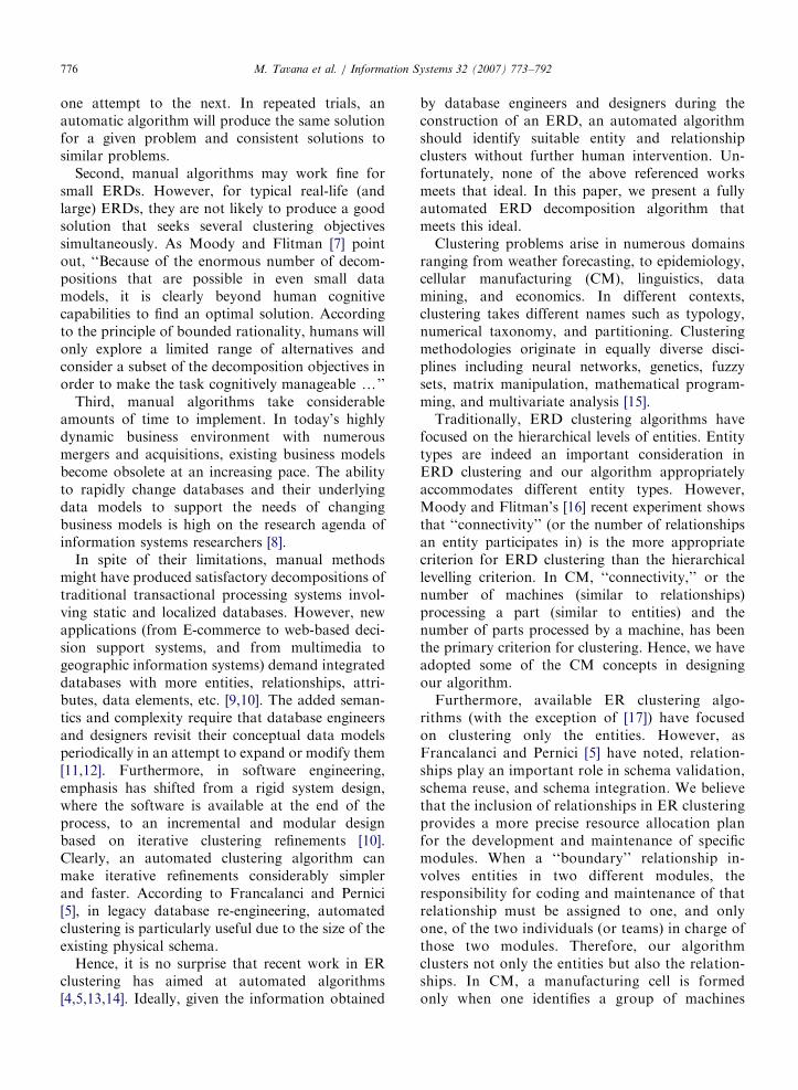
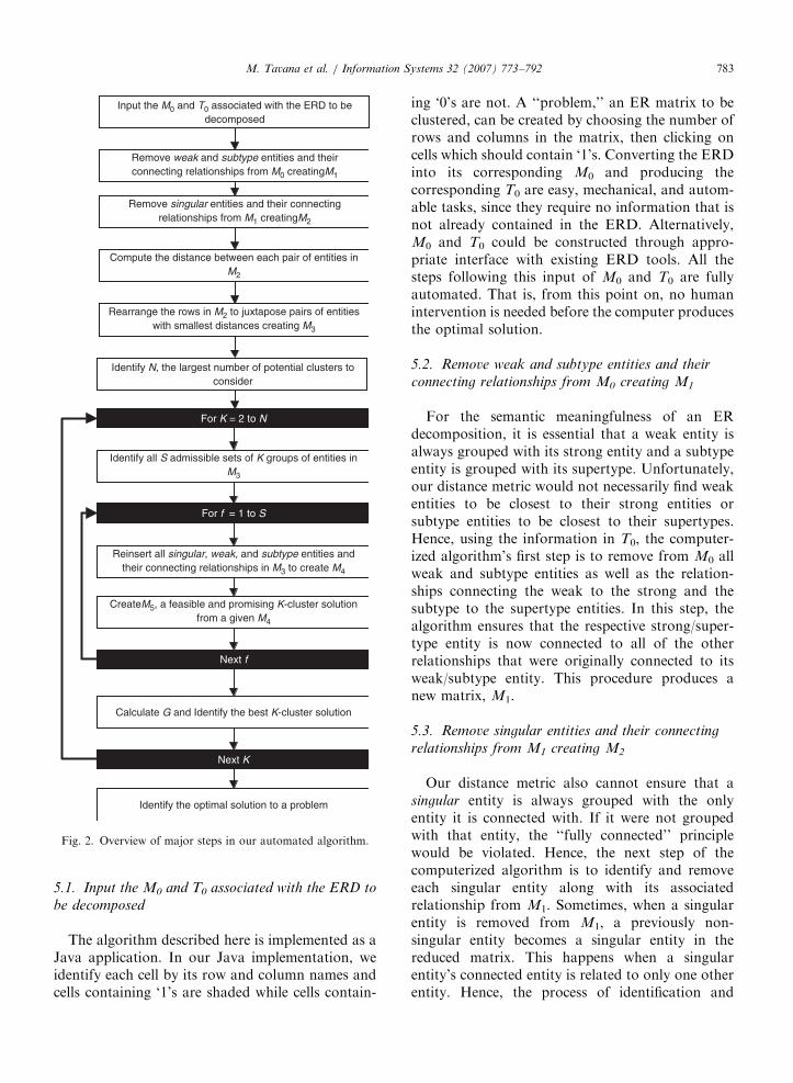
Starting with the M0 and the T0 associated withan ERD, our algorithm consists of eight majorcomputerized steps presented in Fig. 2 and de-scribed in detail below.
ARTICLE IN PRESS
Input the M0 and T0 associated with the ERD to bedecomposed
Identify the optimal solution to a problem
Remove weak and subtype entities and theirconnecting relationships from M0 creatingM1
Calculate G and Identify the best K-cluster solution
Identify all S admissible sets of K groups of entities inM3
Identify N, the largest number of potential clusters toconsider
Rearrange the rows in M2 to juxtapose pairs of entitieswith smallest distances creating M3
Compute the distance between each pair of entities inM2
Remove singular entities and their connectingrelationships from M1 creatingM2
Reinsert all singular, weak, and subtype entities andtheir connecting relationships in M3 to create M4
CreateM5, a feasible and promising K-cluster solutionfrom a given M4
For f = 1 to S
For K = 2 to N
Next f
Next K
Fig. 2. Overview of major steps in our automated algorithm.
M. Tavana et al. / Information Systems 32 (2007) 773–792 783
5.1. Input the M0 and T0 associated with the ERD to
be decomposed
The algorithm described here is implemented as aJava application. In our Java implementation, weidentify each cell by its row and column names andcells containing ‘1’s are shaded while cells contain-
ing ‘0’s are not. A ‘‘problem,’’ an ER matrix to beclustered, can be created by choosing the number ofrows and columns in the matrix, then clicking oncells which should contain ‘1’s. Converting the ERDinto its corresponding M0 and producing thecorresponding T0 are easy, mechanical, and autom-able tasks, since they require no information that isnot already contained in the ERD. Alternatively,M0 and T0 could be constructed through appro-priate interface with existing ERD tools. All thesteps following this input of M0 and T0 are fullyautomated. That is, from this point on, no humanintervention is needed before the computer producesthe optimal solution.
5.2. Remove weak and subtype entities and their
connecting relationships from M0 creating M1
For the semantic meaningfulness of an ERdecomposition, it is essential that a weak entity isalways grouped with its strong entity and a subtypeentity is grouped with its supertype. Unfortunately,our distance metric would not necessarily find weakentities to be closest to their strong entities orsubtype entities to be closest to their supertypes.Hence, using the information in T0, the computer-ized algorithm’s first step is to remove from M0 allweak and subtype entities as well as the relation-ships connecting the weak to the strong and thesubtype to the supertype entities. In this step, thealgorithm ensures that the respective strong/super-type entity is now connected to all of the otherrelationships that were originally connected to itsweak/subtype entity. This procedure produces anew matrix, M1.
5.3. Remove singular entities and their connecting
relationships from M1 creating M2
Our distance metric also cannot ensure that asingular entity is always grouped with the onlyentity it is connected with. If it were not groupedwith that entity, the ‘‘fully connected’’ principlewould be violated. Hence, the next step of thecomputerized algorithm is to identify and removeeach singular entity along with its associatedrelationship from M1. Sometimes, when a singularentity is removed from M1, a previously non-singular entity becomes a singular entity in thereduced matrix. This happens when a singularentity’s connected entity is related to only one otherentity. Hence, the process of identification and
ARTICLE IN PRESSM. Tavana et al. / Information Systems 32 (2007) 773–792784
removal of singular entities is repeated until thereare no singular entities in the modified matrix.Simultaneously, in the order of their removal, a listof all the singular entities and their associatedrelationships is created, so that at the appropriatetime, they can be reinserted in the matrix, in thereverse order of their removal. The resulting matrixis labeled M2. Clearly, if one or more weak, subtype,or singular entities are removed, M2’s dimension,m� n, will be smaller than M0’s dimension (p� q).
5.4. Compute the distance between each pair of
entities in M2
Now, using Eq. (1), our computerized algorithmcomputes the distance between each possible pair ofrows (entities) in M2. As explained in Section 4, theshorter the distance between a pair, the moreappropriate it is to put the two entities in the samecluster, and the larger the distance, the moreappropriate it is to put the two entities in differentclusters.
5.5. Rearrange the rows in M2 to juxtapose pairs of
entities with smallest distances creating M3
Next, our algorithm constructs a matrix, M3,where we leave the relationship columns in the sameorder as in M2, but rearrange the rows so that pairsof entities with least distances are closest to eachother. The algorithm compares all pairwise rowdistances, and copies the pair of rows with the leastdistance next to each other in M3 (arbitrarily one
above the other). Among the UnusedRows, thealgorithm finds the one with the smallest distancefrom one of the current edge rows. The identifiedrow is added to M3 next to that edge row (above thetop edge or below the bottom edge). This process isrepeated until there are no UnusedRows in M2.Thus, at this point, M3 represents the rows in M2, inan order such that the pairs of entity rows with thesmallest distances are closest together.
5.6. Identify N, the largest number of potential
clusters to consider
The next step of the automated algorithm is tofind the range for K, the number of clusters toconsider. As suggested earlier, every cluster mustcontain at least two entities. Hence, the maximumnumber of clusters, N, is the integer value of thenumber of entities divided by two. We also assume
that, when an ER matrix is to be clustered, adatabase manager is looking for at least twoclusters. Therefore, our algorithm assumes that thedesired number of clusters, K, is in [2, N].
5.7. Identify the ‘‘best’’ K-cluster solution for every
possible value of K
This is the most involved part of the algorithmwith several sub-steps detailed below. First, for eachvalue of K ( ¼ 2 to N), the algorithm identifies alladmissible sets (say S) of K groups of entities asdescribed in Section 5.7.1. Next, for each one of theS sets for a given value of K, the algorithm carriesout the sub-steps described in Section 5.7.2 creatingS matrices that are labeled M4. Then, each one ofthe M4’s is used to create a feasible and promisingK-cluster solution as described in Section 5.7.3.Once all S feasible and promising K-cluster solu-tions are created, as described in Section 5.7.4, wecalculate the goodness of fit, G, for each one ofthem. Among the S solutions, the solution with thelargest value of G is identified as the best K-clustersolution.
5.7.1. Identify all S admissible sets of K groups of
entities in M3
Since a matrix’s own boundaries (i.e. the first andthe last rows) also serve as the boundaries for thefirst and the last sub-matrices, respectively, toconstruct a partition resulting in K groups ofentities (rows), we need K�1 other horizontaldividers between rows. It is desirable to draw thedividers between the K�1 pairs of adjacent rowsthat have the greatest distances. However, since acluster must have at least two entities, dividerlocations immediately after the first row, orimmediately before the last row, cannot be con-sidered selectable. Initially, all other possible dividerlocations are considered as selectable. The pair ofadjacent rows with the largest distance is found andthe first divider is placed between those two rows.Since an entity group must contain at least twoentities, entity pairs involving the rows immediatelyadjacent (on either side) to a selected divider are nolonger selectable. Among the remaining pairs ofentities, the pair of adjacent rows with the largestdistance is found and the next divider is placedbetween those two rows. This process is repeatedK�2 times to find all but the last divider. Up untilthis point, ties in largest distances are broken
ARTICLE IN PRESSM. Tavana et al. / Information Systems 32 (2007) 773–792 785
arbitrarily by choosing the first of the tied dividerlocations.
For the (K�1)st divider, often, there are severalselectable divider locations with the same andlargest distance between adjacent rows. Hence, thelast divider is handled differently to ensure thatarbitrary tie-breaking does not cause a bettersolution to be missed. Suppose that there are S
candidates for the (K�1)st divider. Together, thefirst K�2 dividers and one of the S candidatesproduce an admissible set of K groups of entities inM3. Thus, there are S sets of K groups of entities toconsider. Once all S sets of K groups of entities areidentified, for each one of these S sets, the algorithmcarries out the sub-steps described in Sections 5.7.2and 5.7.3.
When, for a given value of K, it is impossible toselect any admissible (K�1)st divider, that value ofK is eliminated from further consideration.
5.7.2. Reinsert all singular, weak, and subtype
entities and their connecting relationships in M3 to
create M4
First, for each admissible set, fAS, of K groups ofentities, the algorithm constructs a new matrix M4
by reinserting, in the reverse order of their removal,each singular, weak, and subtype entity immediatelyabove its respective connected, strong or supertypeentity. If necessary, a divider location is adjusted toensure that the reinserted entity and its relevantentity are in the same group. All the relationshipsare reinserted as the last columns of the matrix andany altered relationship column ‘1’s are adjustedback to their original entity rows. Thus, at the endof this procedure, for each one of the S sets, thecorresponding M4 is a p� q matrix consisting of allthe entities and relationships in M0 and for a givenvalue of K, the total number of M4’s is S.
5.7.3. Create M5, a feasible and promising K-cluster
solution from a given M4
Now, the columns in a given M4 need to berearranged so that each group of entities is clusteredwith suitable relationships. Our aim is to maximizethe goodness of fit of the resulting K-clustersolution. Given the mathematical formula (Eq. (2))for G, to maximize G, one should cluster the largestpossible number of relevant relationships with thesmallest group of entities.
Hence, for each M4, the computerized algorithmcreates a blank matrix, M5, of the same dimensions(p� q) as M4. It copies into M5 all the entity (row)
names in the same order as in M4. The chosen K�1dividers are also copied in M5. Along with thematrix boundaries, the dividers help identify theK groups of entities in M5. Then, an iterativeprocess of column rearrangement and clusteridentification begins.
Each iteration involves first identifying thesmallest group of entities (rows) that has not yetbeen put into a cluster. In case of a tie in the entitygroup size, the first group is selected. The algorithmconsiders each relationship that has not alreadybeen copied to M5. If a relationship has at least asmany 1’s in the rows of the selected group ofentities, as it has in the rows of any of the other un-clustered groups of entities, that relationshipcolumn is copied to matrix M5 in the next availablecolumn spot. When consideration of all relation-ships is done, the copied relationships and theselected group of entities are declared as a cluster,and the algorithm moves on to the identification ofthe next cluster. When all K clusters are constructed,M5 represents the feasible and promising K-clustersolution resulting from a given M4.
As can be noted, this is a greedy procedure formaximizing the G-value of the solution. However,there is no guarantee that an exhaustive approachwould not have found a clustering arrangement witha higher value of G for this set of K groups ofentities. That is why we call this solution as a‘‘feasible and promising’’ solution.
5.7.4. Calculate G and identify the best K-cluster
solution
Once all S feasible and promising K-clustersolutions have been created, the automated algo-rithm calculates the goodness of fit, G, for each oneof them. The solution with the largest value of G isidentified as the best K-cluster solution.
5.8. Identify the optimal solution to a problem
Finally, all the best K-cluster solutions for theentire range of K’s (2 to N) are compared based ontheir G values, and the solution with the highest G ischosen as the ‘‘optimal’’ clustering solution.Although we use the word ‘‘optimal’’ to refer tothe best of the best solutions for various values of K,it should be clear that we are not claiming thatour solution is globally optimal. Our algorithmis a heuristic that employs a greedy approach. Thus,we use the word ‘‘optimal’’ simply to avoid the
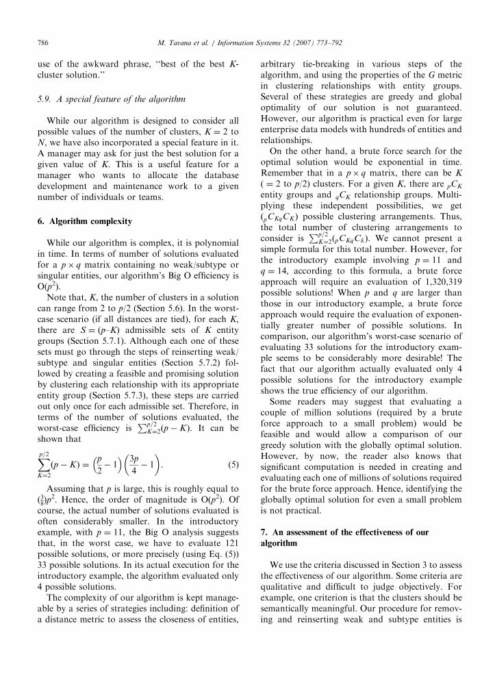
ARTICLE IN PRESSM. Tavana et al. / Information Systems 32 (2007) 773–792786
use of the awkward phrase, ‘‘best of the best K-cluster solution.’’
5.9. A special feature of the algorithm
While our algorithm is designed to consider allpossible values of the number of clusters, K ¼ 2 toN, we have also incorporated a special feature in it.A manager may ask for just the best solution for agiven value of K. This is a useful feature for amanager who wants to allocate the databasedevelopment and maintenance work to a givennumber of individuals or teams.
6. Algorithm complexity
While our algorithm is complex, it is polynomialin time. In terms of number of solutions evaluatedfor a p� q matrix containing no weak/subtype orsingular entities, our algorithm’s Big O efficiency isO(p2).
Note that, K, the number of clusters in a solutioncan range from 2 to p/2 (Section 5.6). In the worst-case scenario (if all distances are tied), for each K,there are S ¼ (p–K) admissible sets of K entitygroups (Section 5.7.1). Although each one of thesesets must go through the steps of reinserting weak/subtype and singular entities (Section 5.7.2) fol-lowed by creating a feasible and promising solutionby clustering each relationship with its appropriateentity group (Section 5.7.3), these steps are carriedout only once for each admissible set. Therefore, interms of the number of solutions evaluated, theworst-case efficiency is
Pp=2K¼2ðp� KÞ. It can be
shown that
Xp=2K¼2
ðp� KÞ ¼p
2� 1
� � 3p
4� 1
� �. (5)
Assuming that p is large, this is roughly equal to(38)p2. Hence, the order of magnitude is O(p2). Of
course, the actual number of solutions evaluated isoften considerably smaller. In the introductoryexample, with p ¼ 11, the Big O analysis suggeststhat, in the worst case, we have to evaluate 121possible solutions, or more precisely (using Eq. (5))33 possible solutions. In its actual execution for theintroductory example, the algorithm evaluated only4 possible solutions.
The complexity of our algorithm is kept manage-able by a series of strategies including: definition ofa distance metric to assess the closeness of entities,
arbitrary tie-breaking in various steps of thealgorithm, and using the properties of the G metricin clustering relationships with entity groups.Several of these strategies are greedy and globaloptimality of our solution is not guaranteed.However, our algorithm is practical even for largeenterprise data models with hundreds of entities andrelationships.
On the other hand, a brute force search for theoptimal solution would be exponential in time.Remember that in a p� q matrix, there can be K
( ¼ 2 to p/2) clusters. For a given K, there are pCK
entity groups and qCK relationship groups. Multi-plying these independent possibilities, we getðpCKqCK Þ possible clustering arrangements. Thus,the total number of clustering arrangements toconsider is
Pp=2K¼2ðpCKqCkÞ. We cannot present a
simple formula for this total number. However, forthe introductory example involving p ¼ 11 andq ¼ 14, according to this formula, a brute forceapproach will require an evaluation of 1,320,319possible solutions! When p and q are larger thanthose in our introductory example, a brute forceapproach would require the evaluation of exponen-tially greater number of possible solutions. Incomparison, our algorithm’s worst-case scenario ofevaluating 33 solutions for the introductory exam-ple seems to be considerably more desirable! Thefact that our algorithm actually evaluated only 4possible solutions for the introductory exampleshows the true efficiency of our algorithm.
Some readers may suggest that evaluating acouple of million solutions (required by a bruteforce approach to a small problem) would befeasible and would allow a comparison of ourgreedy solution with the globally optimal solution.However, by now, the reader also knows thatsignificant computation is needed in creating andevaluating each one of millions of solutions requiredfor the brute force approach. Hence, identifying theglobally optimal solution for even a small problemis not practical.
7. An assessment of the effectiveness of our
algorithm
We use the criteria discussed in Section 3 to assessthe effectiveness of our algorithm. Some criteria arequalitative and difficult to judge objectively. Forexample, one criterion is that the clusters should besemantically meaningful. Our procedure for remov-ing and reinserting weak and subtype entities is
ARTICLE IN PRESSM. Tavana et al. / Information Systems 32 (2007) 773–792 787
designed to partly fulfill this criterion. However,another interpretation of this criterion wouldrequire that the resulting clusters should be capableof being identified as meaningful modules orsubsystems of the larger system. An automaticalgorithm cannot show the semantic meaningfulnessof the resulting clusters by naming the clusters asmeaningful modules. That is a manual task forpracticing database engineers and designers. All wecan report is that we worked on numerous ERDs,and in every case, we have been able to findsemantically meaningful names for the clustersresulting from our algorithm.
Some criteria discussed in Section 3 are absolute.That is, they represent requirements that must bemet by any good clustering solution. Absolutecriteria include ‘‘completeness,’’ ‘‘non-redundancy,’’and ‘‘fully connected’’ principles. Our approach isalgorithmically forced to meet these criteria. Indeed,it was for the ‘‘fully-connected’’ principle that wedeveloped a special procedure to deal with thesingular entities.
Some criteria are relative. They are best discussedin comparison to other methods and in the contextof specific problems. Ideally, we should compare thesolutions to numerous problems obtained by ouralgorithm with the solutions to the same problemsobtained by other algorithms. Unfortunately, mostof the literature discusses general principles ofclustering, using small size examples (involving 8or 9 entities and an even smaller number ofrelationships). We have encountered only twosizable ER clustering problems in the publishedliterature. Next, we present our algorithm’s solu-tions to each one of those problems and comparethem with the solutions to the same problemsobtained by other algorithms.
7.1. Feldman and Miller problem
First, we use Feldman and Miller’s [3, p. 352]problem (Fig. 3). Their solution to this problem ispresented in Fig. 3a. Using Feldman and Miller’sinitial ERD, we constructed a matrix M0 and a tableT0 and used our algorithm to obtain the solutionshown in Fig. 3b.
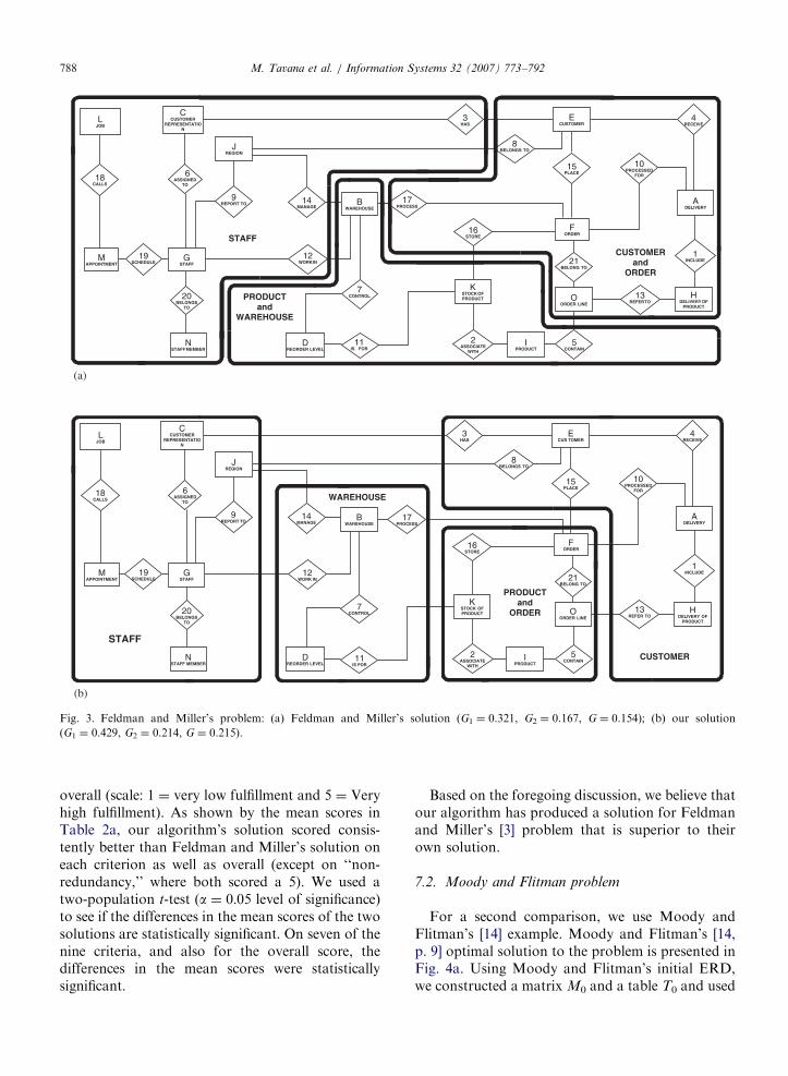
Let us compare the two solutions in Figs. 3a andb on the criteria we have established earlier. First,note that both solutions satisfy the absolute criteriaof completeness, non-redundancy, and fully con-nectedness. Feldman and Miller’s [3] solutionconsists of 3 clusters, while our solution consists
of 4 clusters. Thus, our solution has a higher degreeof modularity. Thus, our solution offers greaterflexibility to a database manager in allocatingmodular tasks to information technology personnel(or teams). Of course, if a manager so desires, twoor more of our clusters could always be assigned toa single team.
One dimension of semantic meaningfulness iswhether or not every weak and subtype entity isclustered with its strong or supertype entity. Ouralgorithm is designed to ensure that. Feldman andMiller’s solution also fulfills this requirement.Another dimension of this criterion is whether ornot the various clusters in a solution are semanti-cally meaningful. We have taken the liberty to namethe clusters in Figs. 3a and b in a semanticallymeaningful way. We find that on both diagrams, allclusters are semantically meaningful. However,notice that in labeling two of the clusters inFeldman and Miller’s solution, in order to beadequately descriptive, we had to use the names oftwo entities each. In contrast, only one of our fourclusters needed the names of two entities. Thus, oursolution fulfils Moody and Flitman’s ‘‘centered’’criterion a little better. However, because in ourview, the ‘‘centered’’ criterion is not very important,and because the semantic meaningfulness of anaming scheme lies in the eye of the beholder, wedo not want to attach too much importance to thesedifferences. We are satisfied that our clusters aresemantically meaningful.
Compared to our solution, Feldman and Miller’ssolution has a smaller number of relationships thatare connected outside their own clusters. This isreflected in the coupling metric, G2, which is 0.167for Feldman and Miller’s solution and 0.214 for oursolution. However, our solution has a substantiallylarger proportion of within-cluster entity pairs thatare directly connected to each other. This is reflectedin the cohesion metric, G1, which is 0.429 for oursolution but only 0.321 for Feldman and Miller’ssolution. Thus, our solution provides a betterbalance between cohesion and coupling, reflectedin the fact that Feldman and Miller’s solution hasa G of only 0.154, whereas our solution attains aG of 0.215.
We also showed Figs. 3a and b (with their titleschanged to ‘‘Solution A1’’ and ‘‘Solution A2,’’respectively, and the labeling of the clusters removedto avoid any bias to our expert database engineersand designers and asked them to assess each solutionon Moody and Flitman’s [7] nine criteria as well as
ARTICLE IN PRESS
Fig. 3. Feldman and Miller’s problem: (a) Feldman and Miller’s solution (G1 ¼ 0.321, G2 ¼ 0.167, G ¼ 0.154); (b) our solution
(G1 ¼ 0.429, G2 ¼ 0.214, G ¼ 0.215).
M. Tavana et al. / Information Systems 32 (2007) 773–792788
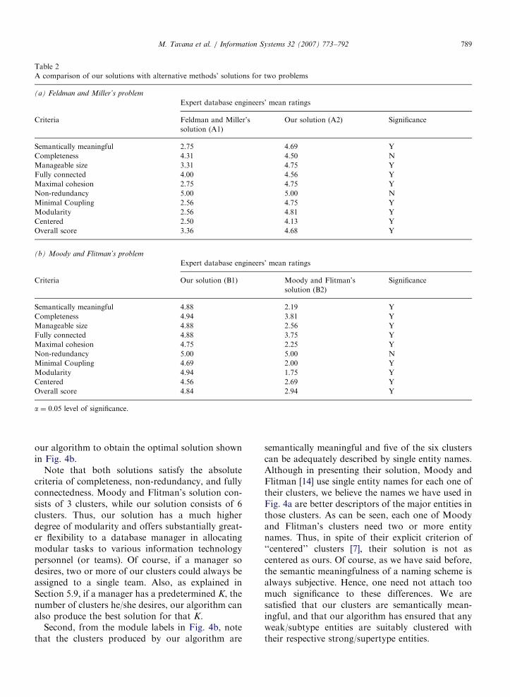
overall (scale: 1 ¼ very low fulfillment and 5 ¼ Veryhigh fulfillment). As shown by the mean scores inTable 2a, our algorithm’s solution scored consis-tently better than Feldman and Miller’s solution oneach criterion as well as overall (except on ‘‘non-redundancy,’’ where both scored a 5). We used atwo-population t-test (a ¼ 0:05 level of significance)to see if the differences in the mean scores of the twosolutions are statistically significant. On seven of thenine criteria, and also for the overall score, thedifferences in the mean scores were statisticallysignificant.
Based on the foregoing discussion, we believe thatour algorithm has produced a solution for Feldmanand Miller’s [3] problem that is superior to theirown solution.
7.2. Moody and Flitman problem
For a second comparison, we use Moody andFlitman’s [14] example. Moody and Flitman’s [14,p. 9] optimal solution to the problem is presented inFig. 4a. Using Moody and Flitman’s initial ERD,we constructed a matrix M0 and a table T0 and used
ARTICLE IN PRESS
Table 2
A comparison of our solutions with alternative methods’ solutions for two problems
(a) Feldman and Miller’s problem
Expert database engineers’ mean ratings
Criteria Feldman and Miller’s
solution (A1)
Our solution (A2) Significance
Semantically meaningful 2.75 4.69 Y
Completeness 4.31 4.50 N
Manageable size 3.31 4.75 Y
Fully connected 4.00 4.56 Y
Maximal cohesion 2.75 4.75 Y
Non-redundancy 5.00 5.00 N
Minimal Coupling 2.56 4.75 Y
Modularity 2.56 4.81 Y
Centered 2.50 4.13 Y
Overall score 3.36 4.68 Y
(b) Moody and Flitman’s problem
Expert database engineers’ mean ratings
Criteria Our solution (B1) Moody and Flitman’s
solution (B2)
Significance
Semantically meaningful 4.88 2.19 Y
Completeness 4.94 3.81 Y
Manageable size 4.88 2.56 Y
Fully connected 4.88 3.75 Y
Maximal cohesion 4.75 2.25 Y
Non-redundancy 5.00 5.00 N
Minimal Coupling 4.69 2.00 Y
Modularity 4.94 1.75 Y
Centered 4.56 2.69 Y
Overall score 4.84 2.94 Y
a ¼ 0.05 level of significance.
M. Tavana et al. / Information Systems 32 (2007) 773–792 789
our algorithm to obtain the optimal solution shownin Fig. 4b.
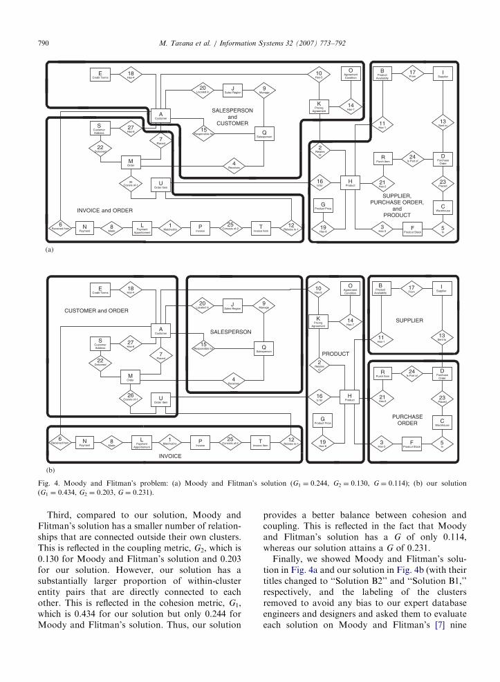
Note that both solutions satisfy the absolutecriteria of completeness, non-redundancy, and fullyconnectedness. Moody and Flitman’s solution con-sists of 3 clusters, while our solution consists of 6clusters. Thus, our solution has a much higherdegree of modularity and offers substantially great-er flexibility to a database manager in allocatingmodular tasks to various information technologypersonnel (or teams). Of course, if a manager sodesires, two or more of our clusters could always beassigned to a single team. Also, as explained inSection 5.9, if a manager has a predetermined K, thenumber of clusters he/she desires, our algorithm canalso produce the best solution for that K.
Second, from the module labels in Fig. 4b, notethat the clusters produced by our algorithm are
semantically meaningful and five of the six clusterscan be adequately described by single entity names.Although in presenting their solution, Moody andFlitman [14] use single entity names for each one oftheir clusters, we believe the names we have used inFig. 4a are better descriptors of the major entities inthose clusters. As can be seen, each one of Moodyand Flitman’s clusters need two or more entitynames. Thus, in spite of their explicit criterion of‘‘centered’’ clusters [7], their solution is not ascentered as ours. Of course, as we have said before,the semantic meaningfulness of a naming scheme isalways subjective. Hence, one need not attach toomuch significance to these differences. We aresatisfied that our clusters are semantically mean-ingful, and that our algorithm has ensured that anyweak/subtype entities are suitably clustered withtheir respective strong/supertype entities.
ARTICLE IN PRESS
Fig. 4. Moody and Flitman’s problem: (a) Moody and Flitman’s solution (G1 ¼ 0.244, G2 ¼ 0.130, G ¼ 0.114); (b) our solution
(G1 ¼ 0.434, G2 ¼ 0.203, G ¼ 0.231).
M. Tavana et al. / Information Systems 32 (2007) 773–792790
Third, compared to our solution, Moody andFlitman’s solution has a smaller number of relation-ships that are connected outside their own clusters.This is reflected in the coupling metric, G2, which is0.130 for Moody and Flitman’s solution and 0.203for our solution. However, our solution has asubstantially larger proportion of within-clusterentity pairs that are directly connected to eachother. This is reflected in the cohesion metric, G1,which is 0.434 for our solution but only 0.244 forMoody and Flitman’s solution. Thus, our solution
provides a better balance between cohesion andcoupling. This is reflected in the fact that Moodyand Flitman’s solution has a G of only 0.114,whereas our solution attains a G of 0.231.
Finally, we showed Moody and Flitman’s solu-tion in Fig. 4a and our solution in Fig. 4b (with theirtitles changed to ‘‘Solution B2’’ and ‘‘Solution B1,’’respectively, and the labeling of the clustersremoved to avoid any bias to our expert databaseengineers and designers and asked them to evaluateeach solution on Moody and Flitman’s [7] nine
ARTICLE IN PRESSM. Tavana et al. / Information Systems 32 (2007) 773–792 791
criteria as well as overall. As Table 2b shows, oursolution scored consistently better than their solu-tion on each criterion as well as overall (except the‘‘non-redundancy’’ criterion, where both solutionsscored 5). The higher scores of our solution werestatistically significant on eight of the nine criteria aswell as the overall score.
In view of the above considerations, we believethat our algorithm has resulted in a substantiallybetter solution than Moody and Flitman’s solutionto their problem.
8. Conclusion and directions for future research
We have described an algorithm for decomposingERDs into manageable modules. Unlike earlierefforts, our algorithm clusters not only the entitiesbut also the relationships involved. In designing thealgorithm, we have capitalized on certain conceptsand metrics from research in CM. At the same time,we exploit some of the unique characteristics ofERDs. Our method is fully automated; that is, usingonly the information contained in an ERD, throughan automated computer procedure, it identifiessuitable entity and relationship clusters withoutany further human (subjective) intervention. Thealgorithm has been implemented as an easy to useJava application, and tested for a variety of sampleproblems. We have discussed how our algorithmfulfills a comprehensive set of criteria for a gooddecomposition of ERDs. We have also comparedour algorithm’s application to two publishedproblems solved by other algorithms. Our algorithmproduces a more cohesive set of clusters whilekeeping inter-cluster coupling small. Our solutionalso offers a higher degree of modularity than thatoffered by other algorithms’ solutions.
While our algorithm produces very good solu-tions, it cannot guarantee their global optimality.First, our goodness of fit metric is not necessarilyperfect. It is the best of several available metrics thatattempt to balance the two objectives of maximizingcohesion while minimizing coupling. Future re-search may produce a better metric that may leadto a better algorithm. Second, in order to keep thecomputational time reasonable, in case of ties, ouralgorithm simply selects one of the choices arbi-trarily. We also use a greedy approach to columnrearrangement and cluster formation.
Nevertheless, our survey of the expert databaseengineers and designers at NASA has shown thatpracticing database engineers and designers find our
solutions preferable to those produced by otheravailable algorithms. Hence, throughout the systemdesign, development, and implementation process,practicing database managers should benefit fromthe manageable modular decompositions of theirERDs produced by our algorithm.
References
[1] P.P. Chen, The entity–relationship model—towards a
unified view of data, ACM Trans. Database Syst. 1 (1)
(1976) 9–36.
[2] R. Maier, Benefits and quality of data modeling—results of
an empirical analysis, in: B. Thalhiem (Ed.), Proceedings of
15th International Conference on the Entity–Relationship
Approach, Springer, Berlin, Heidelberg, 1996, pp. 245–260.
[3] P. Feldman, D. Miller, Entity model clustering: structuring a
data model by abstraction, Comput. J. 29 (4) (1986)
348–360.
[4] J. Akoka, I. Comyn-Wattiau, Entity–relationship and
object-oriented model automatic clustering, Data Knowl.
Eng. 20 (1) (1996) 87–117.
[5] C. Francalanci, B. Pernici, Abstraction levels for entity–
relationship schemas, in: P. Loucopoulus (Ed.), Proceedings
of 13th International Conference on the Entity–Relationship
Approach, Springer, Berlin, Heidelberg, 1994, pp. 456–473.
[6] T.J. Teorey, G. Wei, D.L. Bolton, J. Koenig, ER model
clustering as an aid for user communication and Documen-
tation in database design, Commun. ACM 32 (8) (1989)
975–987.
[7] D. Moody, A. Flitman, A methodology for clustering entity
relationship models—a human information processing
approach, in: J. Akoka, M. Bouzeghoub, I. Comyn-Wattiau,
E. Metais (Eds.), Proceedings of 18th International Con-
ference on the Entity–Relationship Approach, Springer,
Berlin, Heidelberg, 1999, pp. 114–130.
[8] M. Genero, G. Poels, M. Piattini, Defining and validating
metrics for assessing the maintainability of entity–relation-
ship diagrams, Working Papers of Faculty of Economics
and Business Administration: Ghent University—Belgium
03/199, 2003.
[9] A. Badia, Entity–relationship modeling revisited, ACM
SIGMOD Manage. Data Notes 33 (1) (2004) 77–82.
[10] C. Francalanci, A. Fuggetta, Integrating information
requirements along processes: a survey and research direc-
tions, ACM SIGSOFT Software Eng. Notes 22 (1) (1997)
68–74.
[11] S. Castano, V. De Antonellis, M.G. Fugini, B. Pernici,
Conceptual schema analysis: techniques and applications,
ACM Trans. Database Syst. 23 (3) (1998) 286–333.
[12] P. Jaeschke, A. Oberweis, W. Stucky, Extending ER model
clustering by relationship clustering, in: R. Elmasri, V.
Kouramajian, B. Thalheim (Eds.), Proceedings of 12th
International Conference on the Entity–Relationship Ap-
proach, Springer, Berlin, Heidelberg, 1994, pp. 451–462.
[13] S.B. Huffman, R.V. Zoeller, A rule-based system tool for
automated ER model clustering, in: F.H. Lochovsky (Ed.),
Proceedings of 8th International Conference on the Enti-
ty–Relationship Approach, Springer, Berlin, Heidelberg,
1989, pp. 221–236.
ARTICLE IN PRESSM. Tavana et al. / Information Systems 32 (2007) 773–792792
[14] D. Moody, A. Flitman, A methodology for decomposing
entity relationship models—a human information processing
approach, Department of Information Systems Working
Paper, University of Melbourne, Parkville, Victoria, Aus-
tralia, 1999, pp. 1–43.
[15] M. Halkidi, M. Vazirgiannis, Y. Batistakis, Clustering
algorithms and validity measures, Proceedings of 2001
Scientific and Statistical Database Management (SSDBM)
Conference, Virginia, 2001, pp. 3–22.
[16] D.L. Moody, A.R. Flitman, A decomposition method for
entity relationship models: a systems theoretic approach,
International Conference on Systems Thinking in Manage-
ment 2000, in: G. Altmann, J. Lamp, P.E.D. Love, P.
Mandal, R. Smith, M. Warren (Eds.), Proceedings of the
International Conference on Systems Thinking in Manage-
ment, Technical University of Aachen, Geelong, Australia,
2000, pp. 462–469.
[17] J. Akoka, I. Comyn-Wattiau, Framework for automatic
clustering of semantic models, in: R. Elmasri, V. Kourama-
jian, B. Thalheim (Eds.), Proceedings of 12th International
Conference on the Entity–Relationship Approach, Springer,
Berlin, Heidelberg, 1993, pp. 438–450.
[18] J. Martin, Strategies for Data-Planning Methodologies,
Prentice-Hall, Englewood Cliffs, NJ, 1982.
[19] L.J. Campbell, T.A. Halpin, H.A. Proper, Conceptual
schemas with abstractions—making flat schemas more
comprehensible, Data Knowl. Eng. 20 (1) (1996) 39–85.
[20] D.L. Moody, Entity connectivity vs. hierarchical leveling as
a basis for data model clustering: an experimental analysis,
Database Expert Syst. Appl. 2736 (2003) 77–87.
[21] J.L. Burbidge, Production flow analysis, Prod. Eng. 42 (12)
(1963) 742–752.
[22] M.P. Chandrasekharan, R. Rajagopalan, An ideal seed non-
hierarchical clustering algorithm for cellular manufacturing,
Int. J. Prod. Res. 24 (2) (1986) 451–464.
[23] A.J. Vakharia, U. Wemmerlov, A comparative investigation
of hierarchical clustering techniques and dissimilarity
measures applied to cell formation problem, J. Oper.
Manage. 13 (2) (1995) 117–138.
[24] J. Miltenburg, W. Zhang, A comparative evaluation of nine
well-known algorithms for solving the cell formation
problem in group technology, J. Oper. Manage. 10 (1)
(1991) 44–72.
[25] P. Joglekar, M. Tavana, S. Banerjee, A clustering algorithm
for identifying information subsystems, J. Int. Inform.
Manage. 3 (1994) 129–141.
[26] C. Mosier, J. Yelle, G. Walker, Survey of similarity
coefficient based methods as applied to the group technology
configuration problem, Omega 25 (1) (1997) 65–79.
[27] H. Seifoddini, A note on the similarity coefficient method
and the problem of improper machine assignment in group
technology applications, Int. J. Prod. Res. 27 (2) (1989)
1161–1165.
[28] P. Joglekar, Q. Chung, M. Tavana, Note on a comparative
evaluation of nine well-known algorithms for solving the cell
formulation problem in group technology, J. Appl. Math.
Decis. Sci. 5 (4) (2001) 253–268.
[29] S.M. Ng, On the characterization and measure of machine
cells in group technology, Oper. Res. 44 (5) (1996)
735–744.