Embed Size (px)
Citation preview
University of South FloridaScholar Commons
Graduate Theses and Dissertations Graduate School
4-16-2008
A Monte Carlo Approach for Exploring theGeneralizability of Performance StandardsJames Thomas CoraggioUniversity of South Florida
Follow this and additional works at: https://scholarcommons.usf.edu/etd
Part of the American Studies Commons
This Dissertation is brought to you for free and open access by the Graduate School at Scholar Commons. It has been accepted for inclusion inGraduate Theses and Dissertations by an authorized administrator of Scholar Commons. For more information, please [email protected].
Scholar Commons CitationCoraggio, James Thomas, "A Monte Carlo Approach for Exploring the Generalizability of Performance Standards" (2008). GraduateTheses and Dissertations.https://scholarcommons.usf.edu/etd/188
A Monte Carlo Approach for Exploring the
Generalizability of Performance Standards
by
James Thomas Coraggio
A dissertation submitted in partial fulfillment of the requirements for the degree of
Doctor of Philosophy Department of Measurement and Evaluation
College of Education University of South Florida
Major Professor: John M. Ferron, Ph.D. Jeffrey D. Kromrey, Ph.D. Robert F. Dedrick, Ph.D.
Stephen Stark, Ph.D.
Date of Approval: April 16, 2008
Keywords: Standard Setting, Angoff Values, Rater Reliability, Rater Error, Simulation
©Copyright 2008, James Thomas Coraggio

Dedication
This dissertation is dedicated to my immediate family: my wife, Penny, and my
three children, Sydnie, Allyson, and Austin. Penny has been there for me every step of
the way. The journey has at times been difficult and demanding, but her support has been
unwavering. Through it all we have had three children, and earned three degrees and a
national board certification between us. Without her support, understanding, and
devotion, I would not have been able to complete the first page of this dissertation, much
less completed my first class. My two girls have had to endure countless hours away
from their father during the ‘early’ years of their lives. I dedicate this dissertation to both
of them in hopes that the importance of education will be engrained on them for the rest
their lives. Austin is my little ‘miracle’ child. His recent birth has kept me grounded as I
have worked to complete this dissertation. From him, I have learned that God truly does
work in mysterious ways. We can plan all we like, but fate untimely intervenes. As this
journey comes to a completion, I am sure that another will begin very soon. My formal
education is finally over and I hope to make up all that ‘lost’ time with my family.
Girls…daddy’s finally home from school!
Acknowledgements
Many years ago this long and arduous journey of a doctoral degree began with
just a dream and a little imagination. What I have learned along the way is that dreams
can come true, but not without hard work, dedication, and the support of friends and
family. While I would like to thank a number of people for making this opportunity a
reality, I must start with my major professor, Dr. John Ferron. Without his confidence in
my abilities and continued support over the last few years, I know that this dissertation
would not have been possible. As an educator, he will continue to be my role model. In
every opportunity that I have to teach, I will strive to match his patience, compassion,
and understanding. The other members of my committee have been extremely
instrumental in my doctorial preparation as well. Dr Jeffrey Kromrey provided the
understanding and tools need to complete my simulation study, Dr. Robert Dedrick kept
me grounded in the humanistic element of what we do as psychometricians, and Dr.
Stephen Stark provided the in-depth understanding of Item Response Theory.
In addition to the members of my committee, I would like to thank the members
of the Department of Measurement and Research for their assistance. These include our
department manager, Lisa Adkins; current faculty members, Dr. Constance Hines and Dr.
Melinda Hess; and former faculty members, Dr. Tony Onwuegbuzie, Dr. Lou Carey, Dr.
Susan Maller, and Dr. Bruce Hall. Also, I would like to thank my fellow students who
provide support, camaraderie, and encouragement: Amy Bane, Bethany Bell, Garron
Gianopulos, Gianna Rendina-Gobioff, Ha Phan, Jeanine Ramano, and Heather Scott.
Lastly, I would like to thank my former and current employers who encouraged
me to continue my education; Dr. Lee Schroeder, Dr. Elspeth Stuckey, Dr. Beverly Nash,
Dr. Carol Weideman, and Dr. Conferlete Carney.
i
Table of Contents
List of Tables ..................................................................................................................... iv
List of Figures .................................................................................................................. viii
Abstract .............................................................................................................................. xi
Chapter One: Introduction ................................................................................................. 1
Background..................................................................................................................... 1 Appropriate Standard Setting Models......................................................................... 2 Characteristics of the Item Sets .................................................................................. 3 Characteristics of the Standard Setting Process.......................................................... 4
Statement of the Problem................................................................................................ 5 Purpose............................................................................................................................ 6 Research Questions......................................................................................................... 7 Research Hypothesis....................................................................................................... 8 Procedures..................................................................................................................... 10 Limitations .................................................................................................................... 11 Importance of Study...................................................................................................... 11 Definitions .................................................................................................................... 12
Chapter Two: Literature Review ..................................................................................... 15
Introduction................................................................................................................... 15 Standard Setting Methodology ..................................................................................... 15 Current Standard Setting Methods................................................................................ 17
Classical Rational Methods ...................................................................................... 18 Nedelsky ............................................................................................................... 18 Angoff and Modified Angoff Method .................................................................. 19
IRT-Based Rational Methods ................................................................................... 21 Bookmark Method ................................................................................................ 22 Bookmark Variations ............................................................................................ 23
Standard Setting Implications....................................................................................... 24 Issues in the Standard Setting Process.......................................................................... 27
Rater Reliability........................................................................................................ 27 Influence of Group Dynamics................................................................................... 30 Participant Cognitive Processes................................................................................ 33 Identifying Sources of Error ..................................................................................... 36
Previous Simulation and Generalizability Studies........................................................ 36 Previous Simulation Studies ..................................................................................... 36 Previous Studies of Performance Standard Generalizability.................................... 38
Summary of the Literature Review............................................................................... 41
ii
Chapter Three: Method..................................................................................................... 43
Purpose.......................................................................................................................... 43 Research Questions....................................................................................................... 43 Research Hypothesis..................................................................................................... 44 Simulation Design......................................................................................................... 46
Simulation Factors .................................................................................................... 48 Simulation Procedures .................................................................................................. 59
Data Generation ........................................................................................................ 60 Phase 1: Item Main Effect......................................................................................... 61 Phase 2: Rater Main Effect ....................................................................................... 66 Phase 3: Item X Rater Interaction............................................................................. 67 Group Dynamics and Discussion.............................................................................. 69 Individual Item Performance Standard Estimates .................................................... 71
Simulation Model Validation........................................................................................ 74 Internal Sources of Validity Evidence ...................................................................... 74
Sources of Error .................................................................................................... 74 Recovery of Originating Performance Standard................................................... 75 Standard Setting Model Fit to IRT Model ............................................................ 75
External Sources of Validity Evidence..................................................................... 76 Research Basis for Simulations Factors and Corresponding Levels .................... 76 Review by Content Expert .................................................................................... 77 Comparisons to ‘Real’ Standard Setting Datasets ................................................ 77
Phase 3: Item X Rater Interaction............................................................................. 79 Programming................................................................................................................. 79 Analysis ........................................................................................................................ 79
Research Question 1 ................................................................................................. 81 Research Question 2 ................................................................................................. 82
Research Questions....................................................................................................... 84 Results Evaluation ........................................................................................................ 85 Generalizability Comparison I...................................................................................... 86
Bias in Generalizability Comparison I...................................................................... 91 Research Question 1 ............................................................................................. 91 Research Question 2 ............................................................................................. 94
Root Mean Square Error in Generalizability Comparison I ..................................... 95 Research Question 1 ............................................................................................. 95 Research Question 2 ............................................................................................. 99
Mean Absolute Deviation in Generalizability Comparison I ................................. 101 Research Question 1 ........................................................................................... 101 Research Question 2 ........................................................................................... 105
Generalizability Comparison II .................................................................................. 108 Bias in Generalizability Comparison II .................................................................. 113
Research Question 1 ........................................................................................... 113 Research Question 2 ........................................................................................... 114
Root Mean Square Error in Generalizability Comparison II.................................. 116
iii
Research Question 1 ........................................................................................... 116 Research Question 2 ........................................................................................... 120
Mean Absolute Deviation in Generalizability Comparison II ................................ 127 Research Question 1 ........................................................................................... 127 Research Question 2 ........................................................................................... 129
Actual Standard Setting Results Comparison............................................................. 137 Bias in Actual Angoff Dataset Comparison............................................................ 138 RMSE in Actual Angoff Dataset Comparison........................................................ 139 MAD in Actual Angoff Dataset Comparison ......................................................... 141
Results Summary ........................................................................................................ 142 Results Summary for Generalizability Comparison I............................................. 143 Results Summary for Generalizability Comparison II ........................................... 144 Results Summary for the Actual Angoff Dataset Comparison............................... 145
Chapter Five: Conclusions............................................................................................. 147
Research Questions..................................................................................................... 152 Summary of Results .................................................................................................... 153
Generalizability Comparison I................................................................................ 153 Generalizability Comparison II .............................................................................. 153 Actual Angoff Dataset Comparison........................................................................ 154
Discussion................................................................................................................... 154 Generalizability Comparison I................................................................................ 155 Generalizability Comparison II .............................................................................. 159
Limitations .................................................................................................................. 162 Implications ................................................................................................................ 164
Implications for Standard Setting Practice ............................................................. 164 Suggestions for Future Research ............................................................................ 170
Conclusions Summary ................................................................................................ 171
References....................................................................................................................... 174
Appendices...................................................................................................................... 187
Appendix A: Deriving the Indivudal Item Performance Estimates ........................... 188 Appendix B: Preliminary Simulation SAS code........................................................ 190
About the Author ................................................................................................... End Page
iv
List of Tables Table 1. Simulation Factors and the Corresponding Levels ....................................55 Table 2. Example Comparison of Estimated RMSE across Replication Sizes.............................................................................56 Table 3. Mean, Standard Deviation, Minimum, and Maximum Values of the IRT Parameters for the Real Distribution........................................58 Table 4. Mean, Standard Deviation, Minimum, and Maximum Values of the IRT Parameters for the Simulated Distribution based on the SAT with Reduced Variance in b-parameters ......................59 Table 5. Mean, Standard Deviation, Minimum, and Maximum Values of the IRT Parameters for the Simulated Distribution based on the SAT.......................................................................................59 Table 6. Mean, Standard Deviation, Minimum, and Maximum Values of the IRT Parameters for the Simulated Uniform Distribution ................59 Table 7. Simulated Data Sample for Parallel Items .................................................62
Table 8. Simulated Data Sample from Phase One: Item Main Effect .....................62
Table 9. Simulated Data Sample from Phase Two: Rater Main Effect ...................64
Table 10. Simulated Data Sample from Phase Three: Item X Rater Interaction ..................................................................................................65
Table 11. Simulated Data Sample from Discussion Phase ........................................68 Table 12. Comparison of Simulated Angoff Variance Percentages With ‘Real’ Angoff Dataset during Round 1.............................................74 Table 13. Comparison of Simulated Angoff Variance Percentages With ‘Real’ Angoff Dataset during Round 2.............................................75 Table 14. Mean, Standard Deviation, Minimum, and Maximum Values for Outcomes Associated with Generalizability Comparison I .................82
v
Table 15. Eta-squared Analysis of the Main Effects of the Factors in The Simulation for Generalizability Comparison I ...................................84 Table 16. Eta-squared Analysis of the Two-way Interaction Effects of the Factors in the Simulation for Generalizability Comparison I .............................................................85 Table 17. Eta-squared Analysis of the Three-way Interaction Effects of the Factors in the Simulation for Generalizability Comparison I .............................................................86
Table 18. Bias Mean, Standard Deviation, Minimum, and Maximum Values for Sample Size Factor Associated with Generalizability Comparison I...........................................................88
Table 19. RMSE Mean, Standard Deviation, Minimum, and Maximum Values for Item Difficulty Distribution Factor Associated with Generalizability Comparison I...........................................................91
Table 20. RMSE Mean, Standard Deviation, Minimum, and Maximum Values for Placement of the ‘True’ Performance Factor Associated with Generalizability Comparison I ........................................92
Table 21. RMSE Mean, Standard Deviation, Minimum, and Maximum Values for Number of Sample Items Factor Associated with Generalizability Comparison I...........................................................93 Table 22. RMSE Mean, Standard Deviation, Minimum, and Maximum Values for Directional Influence Factor Associated with Generalizability Comparison I...........................................................95 Table 23. MAD Mean, Standard Deviation, Minimum, and Maximum Values for Item Difficulty Distribution Factor Associated with Generalizability Comparison I...........................................................96 Table 24. MAD Mean, Standard Deviation, Minimum, and Maximum Values for Placement of the ‘True’ Performance Factor Associated with Generalizability Comparison I ........................................98 Table 25. MAD Mean, Standard Deviation, Minimum, and Maximum Values for Number of Sample Items Factor Associated with Generalizability Comparison I...........................................................99
vi
Table 26. MAD Mean, Standard Deviation, Minimum, and Maximum Values for Directional Influence Factor Associated with Generalizability Comparison I.........................................................100 Table 27. Mean, Standard Deviation, Minimum, and Maximum Values for Outcomes Associated with Generalizability Comparison II ..............102 Table 28. Conditions for Generalizability II with an Outcome (bias, RMSE, MAD) equal to -1 or Less, or 1 or Greater........................103
Table 29. Eta-squared Analysis of the Main Effects of the Factors in the Simulation for Generalizability Comparison II .......................................104
Table 30. Eta-squared Analysis of the Two-way Interaction Effects of the Factors in the Simulation for Generalizability Comparison II..........................................................105
Table 31. Eta-squared Analysis of the Three-way Interaction Effects of the Factors in the Simulation for Generalizability Comparison II..........................................................107
Table 32. Bias Mean, Standard Deviation, Minimum, and Maximum Values for Directional Influence Factor Associated with Generalizability Comparison II .......................................................108 Table 33. RMSE Mean, Standard Deviation, Minimum, and Maximum Values for Item Difficulty Distribution Factor Associated with Generalizability Comparison II .......................................................110 Table 34. RMSE Mean, Standard Deviation, Minimum, and Maximum Values for Placement of the ‘True’ Performance Factor Associated with Generalizability Comparison II.....................................112 Table 35. RMSE Mean, Standard Deviation, Minimum, and Maximum Values for Directional Influence Factor Associated with Generalizability Comparison II .......................................................114 Table 36. RMSE as a Function of the Placement of the ‘True’ Performance Factor Associated with Generalizability Comparison II ......................................................116 Table 37. MAD Mean, Standard Deviation, Minimum, and Maximum Values for Item Difficulty Distribution Factor Associated with Generalizability Comparison II .......................................................120
vii
Table 38. MAD Mean, Standard Deviation, Minimum, and Maximum Values for Directional Influence Factor Associated with Generalizability Comparison II .......................................................122 Table 39. Estimated MAD as a Function of the Placement of the ‘True’ Performance Standard Factor and the Directional Influences Factor Associated with Generalizability Comparison II ......................................................124
Table 40. MAD as a Function of the Placement of the ‘True’ Performance Factor Associated with Generalizability Comparison II .......................................................126 Table 41. Bias for Sample Size in the Actual Angoff Dataset.................................130
Table 42. RMSE for Sample Size in the Actual Angoff Dataset.............................131 Table 43. MAD for Sample Size in the Actual Angoff Dataset ..............................132
Table 44. Eta-squared Analysis of the Medium and Large Effects of the Factors in the Simulation for Generalizability Comparison I ...........................................................134 Table 45. Eta-squared Analysis of the Medium and Large Effects of the Factors in the Simulation for Generalizability Comparison II..........................................................136
viii
List of Figures Figure 1. Simulation Flowchart.................................................................................57 Figure 2. Distribution of item difficulty parameters (b) for each level of the item difficulty distribution factor ....................................................60 Figure 3. Relationship between the Angoff ratings (probabilities) and the minimal competency estimates (theta) for a given item. ..............69 Figure 4. Outcomes distribution for Generalizability Comparison I ........................83 Figure 5. Estimated bias for small sample size for Generalizability Comparison I...................................................................87 Figure 6. Two-way bias interaction between item difficulty distributions And Small sample sizes for Generalizability Comparison I......................89 Figure 7. Estimated RMSE for item difficulty distributions for Generalizability Comparison I .............................................................91 Figure 8. Estimated RMSE for the placement of the ‘true’ performance standard for Generalizability Comparison I...............................................93 Figure 9. Estimated RMSE for the small sample sizes for Generalizability Comparison I...................................................................94 Figure 10. Estimated RMSE for the directional influences for Generalizability Comparison I...................................................................95 Figure 11. Estimated MAD for item difficulty distributions for Generalizability Comparison I. ............................................................97 Figure 12. Estimated MAD for the placement of the ‘true’ performance standard for Generalizability Comparison I...............................................98 Figure 13. Estimated MAD for the small sample sizes for Generalizability Comparison I...................................................................99 Figure 14. Estimated MAD for the directional influences for Generalizability Comparison I.................................................................101
ix
Figure 15. Outcomes distribution for Generalizability Comparison I. .....................102 Figure 16. Estimated bias for the directional influences for Generalizability Comparison II ...............................................................109 Figure 17. Estimated RMSE for item difficulty distributions for Generalizability Comparison II ...............................................................111 Figure 18. Estimated RMSE for the placement of the ‘true’ Performance standard for Generalizability Comparison II......................112 Figure 19. Estimated RMSE for the directional influences for Generalizability Comparison II ...............................................................114 Figure 20. Estimated RMSE two-way interaction between the placement of the ‘true’ performance standard factor and the directional influence factor for Generalizability Comparison II..........................................................115 Figure 21. Estimated RMSE two-way interaction between the item difficulty distribution factor and the directional influence factor at originating theta of -1 for Generalizability Comparison II..........................................................117 Figure 22. Estimated RMSE two-way interaction between the item difficulty distribution factor and the directional influence factor at originating theta of 0 for Generalizability Comparison II..........................................................118 Figure 23. Estimated RMSE two-way interaction between the item difficulty distribution factor and the directional influence factor at originating theta of 1 for Generalizability Comparison II..........................................................119 Figure 24. Estimated MAD for item difficulty distributions for Generalizability Comparison II..........................................................121 Figure 25. Estimated MAD for the directional influences for Generalizability Comparison II. ..............................................................123 Figure 26. Estimated MAD two-way interaction between the placement of the ‘true’ performance standard factor and the directional influence factor for Generalizability Comparison II. ............124
x
Figure 27. Estimated MAD two-way interaction between the item difficulty distribution and the directional influences factor for Generalizability Comparison II. ..............................................125 Figure 28. Estimated MAD two-way interaction between the item difficulty distribution factor and the directional influence factor at originating theta of -1 for Generalizability Comparison II..........................................................126 Figure 29. Estimated RMSE two-way interaction between the item difficulty distribution factor and the directional influence factor at originating theta of 0 for Generalizability Comparison II..........................................................127 Figure 30. Estimated RMSE two-way interaction between the item difficulty distribution factor and the directional influence factor at originating theta of 1 for Generalizability Comparison II..........................................................128 Figure 31. Estimated bias for small sample sizes for actual Angoff and simulated datasets .............................................................................131 Figure 32. Estimated RMSE for small sample sizes for actual Angoff and simulated datasets .............................................................................132 Figure 33. Estimated MAD for small sample sizes for actual Angoff and simulated datasets .............................................................................133
xi
A Monte Carlo Approach for Exploring the Generalizability of Performance Standards
James Thomas Coraggio
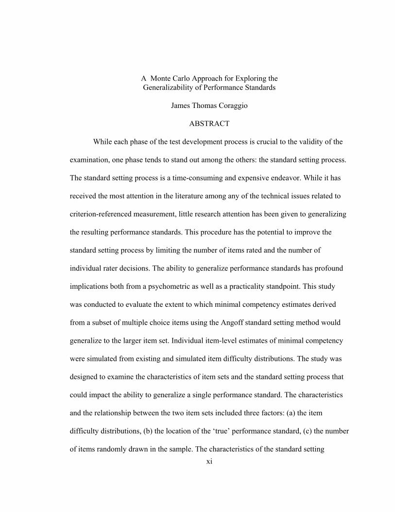
ABSTRACT
While each phase of the test development process is crucial to the validity of the
examination, one phase tends to stand out among the others: the standard setting process.
The standard setting process is a time-consuming and expensive endeavor. While it has
received the most attention in the literature among any of the technical issues related to
criterion-referenced measurement, little research attention has been given to generalizing
the resulting performance standards. This procedure has the potential to improve the
standard setting process by limiting the number of items rated and the number of
individual rater decisions. The ability to generalize performance standards has profound
implications both from a psychometric as well as a practicality standpoint. This study
was conducted to evaluate the extent to which minimal competency estimates derived
from a subset of multiple choice items using the Angoff standard setting method would
generalize to the larger item set. Individual item-level estimates of minimal competency
were simulated from existing and simulated item difficulty distributions. The study was
designed to examine the characteristics of item sets and the standard setting process that
could impact the ability to generalize a single performance standard. The characteristics
and the relationship between the two item sets included three factors: (a) the item
difficulty distributions, (b) the location of the ‘true’ performance standard, (c) the number
of items randomly drawn in the sample. The characteristics of the standard setting
xii
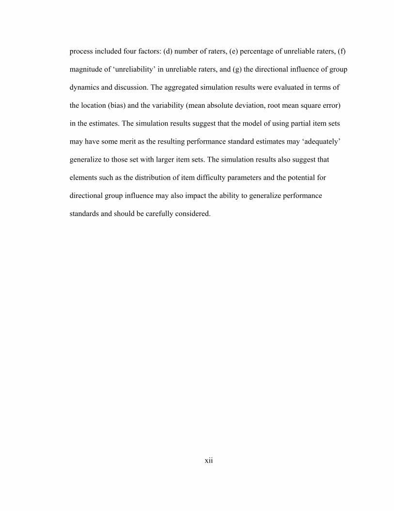
process included four factors: (d) number of raters, (e) percentage of unreliable raters, (f)
magnitude of ‘unreliability’ in unreliable raters, and (g) the directional influence of group
dynamics and discussion. The aggregated simulation results were evaluated in terms of
the location (bias) and the variability (mean absolute deviation, root mean square error)
in the estimates. The simulation results suggest that the model of using partial item sets
may have some merit as the resulting performance standard estimates may ‘adequately’
generalize to those set with larger item sets. The simulation results also suggest that
elements such as the distribution of item difficulty parameters and the potential for
directional group influence may also impact the ability to generalize performance
standards and should be carefully considered.
1
Chapter One:
Introduction
Background
In an age of ever increasing societal expectations of accountability (Boursicot &
Roberts, 2006), measuring and evaluating change through assessment is now the norm,
not the exception. With the establishment of the No Child Left Behind Act of 2001
(NCLB; P.L. 107-110) and the increasing number of “mastery” licensing examinations
(Beretvas, 2004), outcome validation is more important than ever and criterion-based
testing has been the instrument of choice for most situations. Each phase of the test
development process must be extensively reviewed and evaluated if stakeholders are to
be held accountable for the results.
While each phase of the test development process is crucial to the validity of the
examination, one phase tends to stand out among the others: the standard setting process.
It has continually received the most attention in the literature among any of the technical
issues related to criterion-referenced measurement (Berk, 1986). This is largely due to the
fact that determining the passing standard or the acceptable level of competency is one of
the most difficult steps in creating an examination (Wang, Wiser, & Newman, 2001).
Little research attention, however, has been given to generalizing the resulting
performance standards. In essence, can the estimate of minimal competency that is
established with one subset of items be applied to the larger set of items from which it
2
was derived? The ability to generalize performance standards has profound implications
both from a psychometric as well as a practical standpoint.
Appropriate Standard Setting Models
Of the 50 different standard setting procedures (Wang, Pan, & Austin, 2003; for a
detailed description of various methods see Zieky, 2001), the Bookmark method would
seem the method best suited for this type of generalizability due to its use of item
response theory (IRT). In fact, Mitzel, Lewis, Patz, and Green (2001) suggested that the
Bookmark method can “accommodate items sampled from a domain, multiple test forms,
or a single form” as long as the items have been placed on the same scale (p. 253). Yet,
there has been no identifiable research conducted on the subject using the Bookmark
method (Karantonis & Sireci, 2006). While the IRT-based standard setting methods do
use a common scale, they all have a potential issue with reliability. Raters are only given
one opportunity per round to determine an estimate of minimal competency as they select
a single place between items rather than setting performance estimates for each
individual item as in the case of the Angoff method (Angoff, 1971).
The Angoff method and its various modifications are currently one of the most
popular methods of standard setting among licensure and certification organizations
(Impara, 1995; Kane, 1995; Plake, 1998). While the popularity of the Angoff method has
declined since the introduction of the IRT-based Bookmark method, the Angoff method
is still one of the “most prominent” and “widely used” standard setting methods (Ferdous
& Plake, 2005). The Angoff method relies on the opinion of judges who rate each item
according to the probability that a “minimally proficient” candidate will answer a specific
3
item correctly (Behuniak, Archambault, & Gable, 1982). The ratings of the judges are
then combined to create an overall passing standard. The Angoff method relies heavily
on the opinion of individuals and has an inherent aspect of subjectivity that can be of
concern when determining an appropriate standard.
Some limited research on the Angoff method has supported the idea of
generalizing performance standards (Ferdous, 2005; Ferdous & Plake, 2005, 2007; Sireci,
Patelis, Rizavi, Dillingham, & Rodriguez, 2000), and other researchers have suggested
the possibility of generalizing performance standards based only on a subset of items
(Coraggio, 2005, 2007), but before such a process can be implemented, issues such as the
characteristics of the item sets and the characteristics of the standard setting process must
be evaluated for their impact on the process.
Characteristics of the Item Sets
Before a performance standard based on a subset of multiple choice items can be
generalized to a broader set of items, characteristics of the item sets should be addressed.
In other words, how well do the characteristics of the larger item set, the characteristics
of the smaller subset of items, and the relationship between the two item sets impact the
ability to draw inferences from the subset of items? One efficient way to address this
question is to place all the items on the same scale, and the use of item response theory
seems an appropriate psychometric method for this type of analysis. In fact, van der
Linden (1982) suggested that item response theory (IRT) may be useful in the standard
setting process. He suggested that IRT can be used to set estimates of true scores or
expected observed scores for minimally competent examinees (van der Linden, 1982). In
4
fact, some limited research has been conducted placing minimally competency estimates
on an IRT theta scale (see Coraggio, 2005; Reckase, 2006a). In addition to characteristics
of the item sets, the characteristics of the standard setting process may also impact the
ability to accurately generalize performance standards.
Characteristics of the Standard Setting Process
Almost from the introduction of standard setting (Lorge & Kruglov, 1953),
controversy has surrounded the process. Accusations relating to fairness and objectivity
have constantly clouded the standard setting landscape, regardless of the imposed
method. Glass (1978) conducted an extensive review of the various standard setting
methods and determined that the standard setting processes were arbitrary or derived
from arbitrary premises. Jaeger (1989) and Mehrens (1995) found that it was unlikely for
two different standard setting methods to result in comparable standards. Behuniak,
Archambault, and Gable (1982), after researching two popular standard setting models
(Angoff and Nedelsky), had similar results determining that different standard setting
methods produce cut scores that are “statistically and practically different” and even
groups of judges employing the same standard setting method should not be expected to
set similar passing standards (p. 254). “The most consistent finding from the research
literature on standard setting is that different methods lead to different results” (National
Academy of Education, 1993, p. 24). In various research studies, the item difficulty
estimates from raters have been at times inaccurate, inconsistent, and contradictory
(Bejar, 1983; Goodwin, 1999; Mills & Melican, 1988; Reid, 1991; Shepard, 1995;
Swanson, Dillon, & Ross, 1990; Wang et al., 2001). One element that has impacted rater
5
reliability has been the inability for raters to judge item difficulty. While the literature is
well documented with the cause(s) of rater inconsistency, the primary focus of this
research is to explore the resulting impact of rater inconsistency, specifically, as it relates
to the ability to generalize performance standards.
Statement of the Problem
The standard setting process is a time-consuming and expensive endeavor. It
requires the involvement of a number of professionals both as participants such as subject
matter experts (SME) as well as those involved in the test development process such as
psychometricians and workshop facilitators. The standard setting process can also be
cognitively taxing on participants and this has been a criticism of the Angoff method
(Lewis, Green, Mitzel, Baum, & Patz, 1998).
While IRT-based models such as the Bookmark and other variations have been
created to addresses the deficiencies in the Angoff method, research suggests that these
new IRT-based methods have inadvertently introduced other flaws. In a multimethod
study of standard setting methodologies by Buckendahl, Impara, Giraud, & Irwin (2000),
the Bookmark did not produce levels of confidence and comfort with the process that
were very different than the Angoff method. Reckase (2006a) conducted a simulation
study of standard setting processes which attempted to recover the originating
performance standard in the simulation model. He studied the impact of rounding error
on the final estimates of minimal competency for a single rater during a single round of
estimates. His study simulated data using the Angoff and Bookmark methods, and found
that error-free conditions during the first round of Bookmark cut scores were statistically
6
lower than the simulated cut scores (Reckase, 2006a). The estimates of the performance
standard from his research study were “uniformly negatively statistically biased”
(Reckase, 2006a, p. 14). This trend continued after simulating error into rater’s
judgments. These results are consistent with other Bookmark research (Green, Trimble,
& Lewis, 2003; Yin & Schulz, 2005). While the IRT-based standard setting methods do
use a common scale, they all have a potential issue with reliability. Raters are only given
one opportunity per round to determine an estimate of minimal competency as they select
a single place between items rather than setting performance estimates for each
individual item as in the case of the Angoff method. Shultz (2006) suggested a
modification to the Bookmark process that involves the selection of a range of items, but
there is currently little research on this new proposed modification.
Setting a performance standard with the Angoff method on a smaller sample of
multiple choice items and accurately applying it to the larger test form may address some
of these standard setting issues (e.g., cognitively taxing process, high expense, time
consuming). In fact, it may improve the standard setting process by limiting the number
of items and the individual rater decisions. It also has the potential to save time and
money as fewer individual items would be used in the process. Before the
generalizability process can be applied, however, the various issues and implications
involved in the process must be evaluated.
Purpose
The primary purpose of this research was to evaluate the extent to which a single
minimal competency estimate derived from a subset of multiple choice items would be
7
able to generalize to the larger item set. In this context there were two primary goals for
this research endeavor: (1) evaluating the degree to which the characteristics of the two
item sets and their relationship would impact the ability to generalize minimal
competency estimates, and (2) evaluating the degree to which the characteristics of the
standard setting process would impact the ability to generalize minimal competency
estimates.
First, the characteristics and the relationship between the two item sets were
evaluated in terms of their effect on generalizability. This included the distribution of
item difficulties in the larger item set, the placement of the ‘true’ performance standard,
and the number of items randomly drawn from the larger item set. Second, the
characteristics of the standard setting process were evaluated in terms of their effect on
generalizability, specifically, elements such as the number of raters, the ‘unreliability’ of
individual raters in terms of the percentage of unreliable raters and their magnitude of
‘unreliability’, and the influence of group dynamics and discussion. The following
research questions were of interest:
Research Questions
1. To what extent do the characteristics and the relationship between the two item sets
impact the ability to generalize minimal competency estimates?
a. To what extent does the distribution of item difficulties in the larger item set
influence the ability to generalize the estimate of minimal competency?
b. To what extent does the placement of the ‘true’ performance standard influence
the ability to generalize the estimate of minimal competency?
8
c. To what extent does the number of items drawn from the larger item set
influence the ability to generalize the estimate of minimal competency?
2. To what extent do the characteristics of the standard setting process impact the ability to
generalize minimal competency estimates?
a. To what extent does the number of raters in the standard setting process
influence the ability to generalize the estimate of minimal competency?
b. To what extent does the percentage of ‘unreliable’ raters influence the ability to
generalize the estimate of minimal competency?
c. To what extent does the magnitude of ‘unreliability’ in the designated
‘unreliable’ raters influence the ability to generalize the estimate of minimal
competency?
d. To what extent do group dynamics and discussion during the second round of the
standard setting process influence the ability to generalize the estimate of
minimal competency?
Research Hypotheses
1. The following three research hypotheses were related to the research questions
involving the extent to which the characteristics and the relationship between the two
item sets would impact the ability to generalize minimal competency estimates.
a. The distribution of item difficulties in the larger item set will influence the
ability to generalize the estimate of minimal competency. Item difficulty
distributions with a smaller variance in item difficulty parameters will generalize
better than item difficulty distributions with a larger variance.
9
b. The placement of the ‘true’ performance standard will influence the ability to
generalize the estimate of minimal competency. A ‘true’ performance standard
which is closer to the center of the item difficulty distribution will generalize
better than a placement further away.
c. The number of items drawn from the larger item set will influence the ability to
generalize the estimate of minimal competency. The larger the number of items
drawn the better the generalizability of the estimate of minimal competency.
2. The following four hypotheses are related to the research questions involving the extent
to which the characteristics of the standard setting process would impact the ability to
generalize minimal competency estimates.
a. The number of raters in the standard setting process will influence the ability to
generalize the estimate of minimal competency. The larger the number of raters
involved in the standard setting process the better the generalizability of the
estimate of minimal competency.
b. The percentage of ‘unreliable’ raters will influence the ability to generalize the
estimate of minimal competency. Standard setting situations involving a lower
percentage of ‘unreliable’ raters will be able to generalize the estimate of
minimal competency better than those containing a higher number of
‘unreliable’ raters.
c. The magnitude of ‘unreliability’ in the designated ‘unreliable’ raters will
influence the ability to generalize the estimate of minimal competency. Standard
setting situations involving a low magnitude of ‘unreliability’ in the designated
10
‘unreliable’ raters will be able to generalize the estimate of minimal competency
better than those containing a high magnitude of ‘unreliability’ in the designated
‘unreliable’ raters.
d. The group dynamics and discussion during the second round of the standard
setting process will influence the ability to generalize the estimate of minimal
competency. Group dynamics and discussion that influence the raters towards
the center of the rating distribution will generalize better than group dynamics
and discussion that influence the raters towards the outside of the rating
distribution.
Procedures
This research simulated the individual item level estimates of minimal
competency using a Monte Carlo Approach. This approach allowed the control and
manipulation of research design factors. The Monte Carlo study included seven factors in
the design. These factors were (a) shape of the distribution of item difficulties in the
larger item set, (b) the placement of the ‘true’ performance standard, (c) the number of
items randomly drawn from the larger item set, (d) the number of raters in the standard
setting process, (e) the percentage of ‘unreliable’ raters, (f) the magnitude of
‘unreliability’ in the designated ‘unreliable’ raters, and (g) the influence of group
dynamics and discussion during the second round of the standard setting process. The
number of levels for each factor will be described in Chapter Three: Methods.
The ability to ‘adequately’ generalize the performance standard was evaluated in
terms of the differences between the performance standard derived with the larger item
11
set and the performance standard derived with the smaller subset of multiple choice
items. The difference between the originating performance standard and the performance
standard derived with the smaller subset of items was also reviewed. The simulation
results were evaluated in terms of the location of the performance standard (bias) and the
variability of the performance standard (mean absolute deviation, root mean square
error).
Limitations
Based on the design of the study and the level of rater subjectivity involved in the
standard setting process, there are a number of limitations that must be considered when
evaluating the final results of this study. While this study has contained a number of
factors to simulate the standard setting process, additional factors affecting the
subjectiveness of individual raters such as content biases, knowledge of minimal
competency, and fatigue may play a role in determining the final passing standard. These
issues would likely affect the other raters in the standard setting process as well. Another
inherent limitation of the study is the number of levels within each factor. These levels
were selected to provide a sense of the impact of each factor. They were not, however,
intended to be an exhaustive representation of all the possible levels within each factor.
Importance of Study
Many factors must be evaluated before concluding the quality of a standard
setting process. While standard setting issues such as the dependability and replicability
continue to populate the literature, other important issues have been underrepresented.
The issue of generalizability is one such issue, and it is important for two reasons. First, it
12
has the potential to improve the quality of the process by limiting the number of items
and individual rater decisions. By reducing the number of items that a rater needs to
review, the quality of their ratings might improve as the raters are “less fatigued” and
have “more time” to review the smaller dataset (Ferdous & Plake, 2005, p. 186). Second,
it has the potential to save time and money for the presenting agency as well as the raters,
who are generally practitioners in the profession. This savings may then be spent on
improving other areas of the test development process. Reducing the time it takes to
conduct the standard setting process may also result in a different class of more qualified
raters who may have been unable to otherwise participate due to time constraints. In
general, the ability to accurately generalize performance standards may have important
implications for improving the quality of the standard setting process and the overall
validity of the examination.
Definitions
Angoff Method. A popular method of standard setting proposed by William
Angoff in 1971. While Angoff did not originally propose the idea of estimating the
proportion of examinees that correctly respond to an item (see Lorge & Kruglov, 1953),
his original idea (or versions of it) is still one of the most popular models of standard
setting today (Impara, 1995; Kane, 1995; Plake, 1998). The popularity of the Angoff
method has decreased slightly over recent years due to the popularity of the IRT-based
methods.
Angoff Values. The proportion or number (depending on methodology) of
minimally competent examinees predicted to correctly respond to a given item. The
13
individual Angoff values are usually averaged across raters and added across items to
produce a minimum passing score.
Bookmark Method. The IRT-based Bookmark method (Lewis, Mitzel, & Green,
1996) developed by CTB/McGraw Hill was specifically designed to address the
deficiency in the Angoff Method (Horn, Ramos, Blumer, & Maduas, 2000). It is one of a
family of IRT-based rational methods, which include the Bookmark method (Lewis et al.,
1996), the Item Mapping method (Wang et al., 2001), and the Mapmark method (Schultz
& Mitzel, 2005). The Bookmark method was intended to work well with multiple item
types (selected and constructed response) and simplify the cognitive task for raters
(Lewis et al., 1998). It is a multi-round process, similar to the Angoff method. However,
instead of presenting the items in administration order, the Bookmark method uses IRT
b-paramters to order the items according to difficultly in an Ordered Item Booklet (OIB)
from easiest to hardest. The Bookmark method only requires that the rater select the
specific location in the OIB that separates one level of ability from another (Horn et al.,
2000) as opposed to the item-by-item review as in the case of the Angoff method.
Facilitator. The person or persons who conduct the standard setting process.
These test development professionals are often psychometricians.
Minimally Competent Candidate (MCC). A candidate or test taker that possesses
a minimal level of acceptable performance. It is this individual who is conceptualized by
standard setting participants when evaluating test content.
Performance Standard. The performance standard is the “conceptual version of
the desired level of competence” (Kane, 1994, p. 426). The passing score of an
14
examination can be expressed as the “operational version” (Kane, 1994). The
performance standard has also been referred to as the minimal performance level (MPL).
Standard Setting. A process for determining a “passing score” or minimal
acceptable level of performance (Cizek, 1996).
Subject Matter Experts (SME). Individuals who have an expertise in a given
subject area and are “qualified to make judgments” concerning the content (Cizek, 1996,
p. 22). SMEs participate in standard setting workshops and judge items for minimal
performance levels. It is also preferred that SMEs are familiar with one or more
individuals who possess a minimal level of acceptable performance. Subject matter
experts are also referred to as raters, judges, or standard setting participants.
Theta-cut or thetamc. The performance standard represented on a theta scale. A
theta represents an unobservable construct (or latent variable) being measured by a scale.
The theta scale is generally normally distributed, N(0,1), and estimated from item
responses given to test items that have been previously calibrated by an IRT model. The
thetamc is calculated using a procedure designed to link item ratings and estimates of
minimal competency with a common scale (Coraggio, 2005).
15
Chapter Two:
Literature Review
Introduction
The primary purpose of this research was to evaluate the extent to which a single
minimal competency estimate from a subset of multiple choice items could be
generalized to a larger set. Specifically, the two primary goals in this research endeavor
were (1) evaluating the degree to which the characteristics of the two item sets and their
relationship impact the ability to generalize minimal competency estimates, and (2)
evaluating the degree to which the characteristics of the standard setting process impact
the ability to generalize minimal competency estimates. The literature review is separated
into three major sections: types of standard setting methods, issues within the standard
setting process, and previous research studies in the areas of standard setting simulation
and generalizing performance standards.
Standard Setting Methodology
As previously alluded to in the introduction of the paper, measuring and
evaluating change through assessment is now the norm in our society, not the exception.
Test developers and psychometricians are now held to tight levels of accountability and
legal defensibility. Every stage of the test development process is evaluated for its
contribution to the reliability of the resulting scores and the validity of the interpretation
of those scores. Of all the stages, the standard setting process has received the most
16
attention in the literature (Berk, 1986). It has been documented that the standard setting
process is one of the most difficult steps (Wang et al., 2001) and may also be one of the
most unreliable (Jaeger, 1989b).
While some standards are still set unsystematically without consideration of a
particular criterion (Berk, 1986), such as setting an arbitrary predetermined passing score
(e.g., score of 70) or establishing a passing standard with a relative standard (quota or an
examinee’s normative performance level) (Jaeger, 1989a), the current accepted standard
setting practices involve the use of an absolute or criterion-referenced process to evaluate
the examination items and set an appropriate passing standard. Reckase (2005) stated that
“a standard setting method should be able to recover the intended standard for a panelist
who thoroughly understands the functioning of the test items and the standard setting
process, and who makes judgments without error” (p. 1). Some researchers, however, do
not share in Reckase’s perspective and warn that a “true” standard or a “best” standard
setting practice may not actually exist (Wang et al., 2003).
Almost from the introduction of standard setting (Lorge & Kruglov, 1953),
controversy has surrounded the process. Accusations relating to fairness and objectivity
have constantly clouded the standard setting landscape, regardless of the imposed
methodology. Glass (1978) conducted an extensive review of the various standard setting
methods and determined that the standard setting processes were either arbitrary or
derived from arbitrary premises. Jaeger (1989b) and Mehrens (1995) found that it was
unlikely for two different standard setting methods to result in comparable standards.
Behuniak, Archambault, and Gable (1982), after researching two popular standard setting
17
methods of the time (Angoff and Nedelsky), had similar results determining that different
standard setting methods produce cut scores that are “statistically and practically
different” and even groups of raters employing the same standard setting method should
not be expected to set similar passing standards (p. 254).
Current Standard Setting Methods
In 1986, Berk claimed that there were more than 38 different methods developed
to estimate passing standards; by 2003, Wang et al. claimed that there were more than 50
different standard setting procedures (For a detailed description of various methods see
Zieky, 2001). Yet, with all the methods available, which methods provide the best
results? “The most consistent finding from the research literature on standard setting is
that different methods lead to different results” (National Academy of Education, 1993,
p. 24).
Due to their increased psychometric rigor and legal defensibility, the absolute or
criterion-based methods are currently the most widely applied standard setting methods.
Three of the most popular types of absolute or criterion-based methods include the
classical rational methods, based on evaluation of test content such as the Nedelsky
(1954) and the Angoff (1971) method (or modified variations); the IRT-based rational
methods such as the Bookmark method (Lewis et al., 1996), Item Mapping method
(Wang et al., 2001), and Mapmark method (Schultz & Mitzel, 2005); and the empirical
methods, based on the examinee distribution on some external criterion such as the
Comparison Groups method, (Livingston & Zieky, 1982) and the Borderline Groups
method (Livingston & Zieky, 1982). Due to the lack of an existing external criterion in
18
most instances, the focus of this research will be on one of the classical rational methods.
Classical Rational Methods
The classical rational methods rely on the expert judgment of raters. These raters
conduct a detailed analysis of each item on the examination in order to establish the
minimal performance standard (Muijtjens, Kramer, Kaufman, & Van der Vleuten. 2003).
Nedelsky. The Nedelsky method has declined in popularity since the introduction
of the IRT-based standard setting methods. It focuses on the minimally competent
candidate and requires a review of every item on the examination, similar to the Angoff
method. Rather than estimating a probability based on the overall difficulty of the item,
the rater instead focuses on the individual item’s multiple choice options and eliminates
those that a minimally competent candidate would recognize as incorrect. An individual
item probability is then determined from the remaining items (e.g., two remaining options
would result in a .50 probability). The individual item probabilities are then averaged
across raters and then summed across items to determine the passing standard. This
process is sometimes conducted over multiple rounds.
The Nedelsky method, while less cognitively taxing for raters than other methods,
does have some inherent weaknesses. It results in a limited number of item probabilities
based on the number of multiple choice options. This may not reflect normal test taking
behavior by a minimally competent candidate. It is also limited to use with multiple
choice style examinations. In comparisons between the Nedelsky and Angoff methods,
The Angoff method produced less variability among individual rater estimates (Brennan
& Lockwood, 1979).
19
Angoff and Modified Angoff Method. Angoff’s method is still one of the most
popular models of standard setting today (Impara, 1995; Kane, 1995; Plake, 1998),
though the popularity of the Angoff method has decreased in recent years due to the
popularity of the IRT-based methods.
Angoff proposed his idea for standard setting in a book chapter entitled, Educational
Measurement. It is important to note that Angoff “unfailingly attributed” the development of
his standard setting method to Ledyard Tucker even though the method and its modified
versions are given only his namesake (Smith & Smith, 1988, p. 259). An original description
of the Angoff procedure is reproduced here (Angoff, 1971, p. 515).
A systematic process for deciding on the minimum raw scores for passing
and honors might be developed as follows: Keeping the hypothetical
‘minimally acceptable person’ in mind, one could go through the test item by
item and decide whether such a person could answer correctly each item
answered correctly by the hypothesized person and a score of zero is given
for each item answered incorrectly by that person, the sum of the item scores
will equal the raw score earned by the ‘minimally acceptable person.’ A
similar procedure could be followed for the hypothetical ‘lowest honors
person.’
This original Angoff method has been described as the Angoff Yes/No
method. While it has been used with some success (see Impara & Plake, 1997), it is
not as popular as his next suggestion. In a footnote on that same page, Angoff
described a variation to the procedure that became known as the Modified-Angoff
20
Approach to standard setting (Reckase, 2000). Below, the footnote from that page is
reproduced (Angoff, 1971, p. 515).
A slight variation of this procedure is to ask each judge to state the
probability that the ‘minimally acceptable person’ would answer each item
correctly. In effect, the judges would think of a number of minimally
acceptable persons, instead of only one such person, and would estimate the
proportion of minimally acceptable persons who would answer each item
correctly. The sum of these probabilities, or proportions, would then
represent the minimally acceptable score.
Impara and Plake (1997) conducted a study of both versions that Angoff
originally proposed. Their results indicated that the Angoff Yes/No version, while not as
popular, produced similar cut score results, was easier to understand for raters, and was
easier to use (Impara & Plake, 1997).
Angoff provided no rationale for either of his standard setting methods (Impara &
Plake, 1997) and this omission may have led to the many variations of his method that
exist today. The Angoff method has been continually adjusted and modified during its
history. In fact, Reckase (2000) stated that “there is no consensus on the definition for the
modified Angoff process” (p. 3).
As shown from the passages, the Angoff models rely on the opinion of raters who
rate each item according to the probability that a “minimally proficient” candidate will
answer a specific item correctly (Behuniak et al., 1982). This can be seen as an advantage
or as a weakness in this particular method. The Angoff method consists of an item-by-
21
item rating method similar to the Nedelsky method, but instead of eliminating options,
the Angoff method requires participants to indicate the proportion of minimally qualified
students who would answer each item correctly based on the difficulty of the item
(Reckase, 2000). As with the Nedelsky method, the item ratings are then averaged across
raters and combined to create an overall passing standard. The Angoff method generally
involves a multi-round process that involves individual ratings as well as group
discussion to achieve the final passing standard.
Regardless of the modification, the Angoff method relies heavily on the opinion of
individuals and has an inherent aspect of subjectivity that can be of concern when
determining an appropriate standard. In fact, it has been described as “fundamentally
flawed” in an evaluation of the standard setting process used with the National Assessment
of Educational Progress (Pellegrino, Jones, & Mitchell, 1999). IRT-based models were
created to address the limitations in the Angoff-based standard setting models.
IRT-Based Rational Methods
In 1982, van der Linden suggested that item response theory (IRT) may be useful in
the standard setting process. Yet, limitations with computer technology at the time may have
limited the usefulness of IRT during the standard setting workshop process. Modern
computer processing speeds and advancement in software have allowed the development of
IRT-based standard setting methods designed to improve on the weaknesses in the Angoff
method. The IRT-based Bookmark method was specifically designed to address the item-by-
item review of the Angoff method (Horn et al., 2000).
22
Bookmark Method. The Bookmark method was intended to work well with multiple
item types (selected and constructed response) and simplify the cognitive task for raters
(Lewis et al., 1998). It is a multi-round process, similar to the Angoff and Nedelsky methods.
However, instead of presenting the items in the order of administration, the Bookmark
method uses IRT parameters to order the items according to difficultly from easiest to
hardest in an Ordered Item Booklet (OIB). The Bookmark method only requires that the rater
select the specific location in the OIB that separates one ability level from another (Horn et
al., 2000) as opposed to the item-by-item review as in the case of the Angoff method.
Specifically, the rater is to select the item location for which a minimally competent
examinee is expected to have mastered the items below, and conversely, not have mastered
the items above (Karantonis & Sireci, 2006). This location is based on a response probability
(RP). The RP is the location selected by the standard setting participant where the examinee
“has a .67 (2/3) probability of success with guessing factored out” (Lewis et al., 1998, p. 3).
By selecting a location where the Bookmark is at the “furthest most item” where this RP is
true, a unique location on the ability scale can be estimated and a cut score established (Lee
& Lewis, 2001, p. 2). The RP of .67 has been traditionally used due to its ease of
understanding for participants (Williams & Schultz, 2005), and its maximizing of the
information function in the 3PL IRT model (Huynh, 2000).
The Bookmark method has become increasingly popular for its simplicity. Raters
only need to focus on the performance of the “barely proficient” examinee without
concern in estimating item difficulty, and raters can perform the required tasks in a much
shorter amount of time (Buckendahl, Impara, Giraud, & Irwin, 2000). The Bookmark
23
method has rapidly grown in popularity from use in 18 states in 1996 (Lee & Lewis,
2001) to use in 31 states in 2005 (Perie, 2005).
In a study comparing the Bookmark and the Angoff methods, Buckendahl et al.
(2000) found that while the two methods produced a similar cut score and similar levels
of confidence and comfort with the process, the Bookmark method had a lower standard
deviation. While they did not conduct a statistical significance test on the differences,
they did suggest that this lower standard deviation would indicate a higher level of inter-
rater agreement to a policy making body (Buckendahl et al., 2000). One element that may
have impacted their results was that their study used Classical Test Theory p-values to
create the OIB as opposed to IRT parameters. Other multiple method studies indicate that
the Bookmark method consistently produces the lowest cut score among standard setting
methods (Green et al., 2003; Yin & Schultz, 2005).
Bookmark Variations. One variation of the Bookmark method is the Item
Mapping Method (Wang et al., 2001). In this method, items are sorted according to
difficulty (using the IRT b-paramters) based on the Rasch IRT model. A rater examines
the items and determines which items a minimally competent candidate would have a .50
probability of answering correctly as opposed to the .67 response probability associated
with the Bookmark method.
Another very recent variation of the Bookmark method is the Mapmark method
(Schultz & Mitzel, 2005) developed by ACT, Inc. It was recently implemented on the
Grade 12 National Assessment of Educational Progress (NAEP) Math test, perhaps in
response to the reported “flaws” in the Angoff method. The Mapmark uses “item maps”

24
(graphical relationships of the items to the proficiency distribution, arranged by content
domains) and content domain scores to assist in “significant” discussion about what
knowledge, skills, and abilities (KSAs) are being measured (Karantonis & Sireci, 2006).
Due to its recent development and single implementation at this point, research on the
Mapmark method has been limited.
Yin and Schultz (2005) conducted a study and compared the Mapmark method
with the Angoff-based method. Their results suggest that the Mapmark cut scores are
lower than those from the Angoff-based method. These results are similar to research
findings from the Bookmark method (Green et al., 2003; Yin & Schultz, 2005). Yin and
Schultz (2005) also discovered that the individual rater cut scores from the Mapmark
method were not normally distributed and contained more extreme scores. In fact, due to
the differences, the median cut score has been used as the final performance standard as
opposed to the mean cut score (Yin & Schultz, 2005). One weakness of all the IRT-based
standard setting methods is that they require large amounts of prior performance data in
order to calibrate the items and create the OIB. The specific amount of required prior
performance data depends on the IRT model employed (e.g., 3PL vs. Rasch).
Standard Setting Implications
Even if the standard setting process has been properly conducted, the resulting
passing standard may have an overall impact (pass/fail rate) that is inconsistent with the
expectations of the raters and/or the policy makers (Buckendahl et al., 2000). It is the
policy makers, not the raters, who determine the final performance standard (Shepard,
1995). It is critical that policy makers take into account “uncertainty” associated with cut
25
scores before adopting a new performance standard (Lewis, 1997).
Often these policy makers may change the resulting cut score only a few raw
score points. While this may seem trivial, a change of a few raw score points may have
significant implications. For example, a change of two raw-score points on a statewide
administration of the National Teaching Examination (NTE) mathematics subtest in April
1983 would have resulted in an additional 13% of examinees not passing the assessment
(Busch & Jaeger, 1990). Another consideration is the impact (pass/fail rate) on minority
groups generally referred to as differential selection. Testing can result in differential
selection rates from groups with different group means (Stark, Chernyshenko, &
Drasgow, 2004). Setting a high cut score can result in an adverse impact on minority
groups and the resulting underselection can result in “contentions” of discrimination
(Stark et al., 2004, p. 497).
From a measurement perspective, this issue of differential selection becomes one
of discerning between differences due to ability (referred to as “impact” in the
measurement literature) and differences due to some assessment measurement bias. The
discussion of measurement bias and the differences between impact and bias are outside
the scope of this particular paper (for a detailed discussion on measurement bias and
impact, see Stark et al., 2004).
From a legal perspective, the issue of differential selection is the perception of
discrimination. This legal discussion specifically addresses the use of performance
standards in certification and licensure applications.
26
The federal Uniform Guidelines on Employee Selection Procedures state the
following:
A selection rate for any race, sex, or ethnic group which is less than four-
fifths (4/5) (or eighty percent) of the rate for the group with the highest
rate will generally be regarded by the Federal enforcement agencies as
evidence of adverse impact, while a rate greater than four-fifths rate will
generally not be regarded by Federal enforcement agencies as evidence of
adverse impact (Equal Employment Opportunity Commission, 1978).
The 4/5th rule, as it is commonly known, basically states that the proportion of
examinees selected from a minority (focal) group at the selected cut score when
compared with the proportions of examinees selected from a majority (reference) group
at the selected cut score can not exceed a ratio of .80. This rule places a significant
amount of legal burden and potential liability on the policy makers in the fields of
licensing and certification in terms of the location of the final performance standard.
While there was no direct evidence in the literature of this rule currently being applied to
the performance standards in educational testing, it might only be a matter of time in this
environment of ever increasing accountability.
Aside from this issue of differential selection, policy makers are also very
concerned with the perceptions of their stakeholders: specifically, the taxpayers in the
case of educational testing, and licensees in the case of accreditation testing. The
resulting performance standard may be “impractical,” providing a performance standard
that is set too high (low pass rate) or too low (high pass rate). This may bring the validity
27
of the examination program in to question.
Issues in the Standard Setting Process
Kane (1994, 2001) proposed three types of validity evidence to be used for
validating performance standards. They were procedural, internal, and external.
Procedural validity evidence focuses on the appropriateness of procedures and quality of
implementation (Kane, 1994). Internal validity evidence focuses on the ability of raters to
translate the performance standard into a passing score (Kane, 1994). He suggested
examining this evidence empirically through the standard error of the cut score. External
validity evidence involves external comparisons such as consistency of cut scores across
different methods or congruence with external examinee classifications (Kane, 1994).
Kane’s validity model claims to provide a way to evaluate the evidence of
validity in the standard setting process, but it focuses primarily on the consistency and
reliability of the process with only limited consideration to whether the resulting
performance standard is truly valid.
Rater Reliability
Individual rater differences were defined in the literature as a threat to standard
setting validity (Sato 1975; van der Linden, 1982; Jaeger, 1988). In discussing these
differences, van der Linden (1982) coined the term ‘intrajudge inconsistency’ when
referring to individual rater error. This term specifically refers to the inconsistency
between item ratings and their associated difficulty (Plake, Melican, & Mills, 1991). For
example, a rater assigns a low probability of success to an easy item and a high
probability of success to a hard item. Engelhard and Cramer (1992) concluded that most
28
of the variation was related to judge inconsistency and this related directly to the
inconsistency within the ratings of specific judges. Their research raised a concern about
the subjectivity of specific judges (Engelhard & Cramer, 1992). Berk (1996) suggested
using intrajudge reliability across consecutive rounds as one criterion for establishing the
quality of the standard setting process. Berk also suggested evaluating rater variance in
the final cut score as another criterion of success (Berk, 1996).
Another approach to identifying rater unreliability was used by Plake and Impara
(2001). They sought to understand how well the raters could estimate the item-level
performance of examinees at the established minimal performance standard. Their study
compared the raters’ estimation of the item-level minimal passing standard with the item-
level performance of actual candidates who had scores close to the raters’ overall
estimation of the minimal performance standard. Their research indicates that the average
difference between actual and anticipated performance was -.002 with a standard
deviation of .09 (Plake & Impara, 2001). One limitation of this approach is that actual
performance values are used as opposed to a ‘true’ value of the minimal performance
standard, which is usually never known. Reckase (2006a) in his simulation study used
these estimates to postulate that raters have an error distribution with a standard deviation
of .1. He used this assumption to stimulate rater error in his simulation model.
Operationally, he proposed that the rater had a 95% chance of estimating the probability
of a correct response within .2 of the intended performance standard or cutscore
(Reckase, 2006a). In other words, if the estimated probability of a correct response for a
given item on the IRT theta scale was .7 based on a true performance standard, then the
29
raters estimate would be between .5 and .9 95% of the time.
One element that has impacted rater reliability (or rater unreliability) has been the
inability for raters to judge individual item difficulty. In various research studies, the item
difficulty estimates from raters have been at times inaccurate, inconsistent, and
contradictory (Bejar, 1983; Goodwin, 1999; Mills & Melican, 1988; Reid, 1991;
Shepard, 1995; Swanson et al., 1990; Wang et al., 2001). While raters are able to
distinguish between which items were easy and which items were hard, they have had
difficulty correctly estimating item difficulty (Shepard, 1995).
This is especially true of estimating item difficulty for minimally competent
examinees and this has resulted in either overestimations of minimally competent
performance or underestimations of minimally competent performance depending on the
items on the examination (Shepard, 1995). One of the main concerns, especially in the
Angoff model, has been the ability of raters to “predict” the performance of minimally
competent candidates (Irwin, Plake, & Impara, 2000). Raters tend to only think of
average examinees as opposed to those that are minimally competent (Bowers &
Shindoll, 1989). Shepard (1995) felt raters were essentially unable to estimate the
response of the minimally competent candidates. Impara and Plake (1997) conducted a
study of two different versions of the Angoff method. Their research suggests that raters
found the conceptualization of a ‘single’ minimally competent examinee easier to
comprehend than imagining a ‘group’ of minimally competent examinees as is prescribed
in the method.
30
Another issue may be a rater’s preconceived perceptions of impact prior to the
workshop. Buckendahl et al. (2000) examined the consequences of a rater’s advanced
estimates of impact. They first asked raters their perceptions of a passing rate and then
provided passing rate information from previous administrations. What they found was
limited evidence to suggest that these early estimates may influence the change and
directionality of ratings between rounds (Buckendahl et al., 2000). Jaeger (1982) found
evidence to suggest that a rater’s background may also have some influence on rater
consistency: specifically, the relationship between the rater’s background and specific
content on the examination (Plake et al., 1991).
Incorporating IRT into the standard setting process may improve the precision of
the process by assisting in examining rater variability (van der Linden, 1982). IRT can be
used to set estimates of true score or expected observed score for minimally competent
examinees (van der Linden, 1982). IRT can also be used to identify the variability of item
difficultly estimates for individual raters. Raters with extreme ratings and raters who
were inconsistent in terms of their definition of minimal competency based on their item
ratings can be identified using IRT (Kane, 1987).
Influence of Group Dynamics
Variability among group participants may account for differences in standard
setting results. Livingston (1995) in a study of the Angoff method reported a likely
group-influenced biasing effect of regression to the mean. Hertz and Chin (2002), after
studying group variability, proposed that standard setting studies should focus on the
interaction among groups as well as on group instruction (training) and individual rater
31
differences. They proposed that the best model for standard setting should be one that
minimizes the effect of the group and simplifies the process (Hertz & Chin, 2002). One
unique study by Wiley and Guille (2002) looked at an occasion effect for participants that
established their judgments individually without any type of group interaction. While the
mean difference between the collaborative group and the “at-home” raters was only 1.20
points, the “at-home” ratings did have more variability and resulted in a slight item-
occasion interaction. The design of the study may also have tempered the results. “At-
home” raters were experienced with the Angoff standard setting process and had access
to 13 anchor items that had previously been rated. While additional research is needed on
the subject of group influence, this study suggests an impact of group interaction on the
resulting performance standard. Group variability is likely influenced by the social
interactions during the standard setting discussion process.
Most standard setting methods include some type of social interaction among
participants, with many of the models requiring multiple rounds of discussion before the
final minimum passing score is determined. Multiple consecutive rounds of ratings are
designed to “foster convergence of views” as the workshop progresses (Karantonis &
Sireci, 2006). Some researchers even suggest providing normative information on
examinee test performance to assist raters in adjusting judgments between rounds (Cizek,
1996). Research on this issue suggests that providing this information to raters will
produce “small and inconsistent” changes in the overall mean performance standard, but
will result in lower rater variability (Busch & Jaeger, 1990, p. 148). Rater cut score
variability has been used as criterion for determining the quality of the standard setting
32
process (Berk, 1996).
One relevant factor that may provide some of the inconsistencies in standard
setting results is social influences (Hertz & Chinn, 2002). Group discussion and
interaction can dramatically change individual perceptions about the difficulty of an item,
and some individuals are more prone than others to change their perceptions. Some raters
have reported feeling pressured to change their original ratings (McGinty, 2005). In fact,
the opinion of the group is on average more extreme after the group discussion, than it is
before the group discussion (Fitzpatrick, 1989). The minority position also may have a
difficult time convincing the majority position during a discussion. The “most likely
result” is for the minority group to give in to the majority position (Hertz & Chinn, 2002,
p. 6). Group discussion has resulted in lower rating variability, and this lower variability
has been traditionally used by practitioners as one measure of standard setting quality.
Raters in the same group employing the same standard setting method had ratings that
were more similar than raters in different groups employing the same method (Behuniak
et al, 1982). One meta-analysis on different variations of the Angoff method resulted in
higher degree of consensus and a higher overall minimal passing standard when
participants focus on a common definition of minimal competency and discuss their
individual estimates as a group (Hurtz & Auerbach, 2003). This higher degree of
consensus may be due to the influence of the dominant interactions by the majority
group. Improving the reliability does not necessarily imply improving the validity of the
passing standard. An issue even bigger than the reliability of the standard setting process,
may be the validity (McGinty, 2005). Researchers tend to focus more on reliability
33
because it can be “more easily” established and researchers are more “comfortable” with
the idea of replicability.
The literature on standard setting has presented several suggestions for improving
the reliability and replicability of the standard setting process. These suggestions include
selecting qualified raters, using proper rater training on procedures and providing a clear
definition of minimal candidate competency (Mills, Melican, & Ahluwalia, 1991; Plake
et al., 1991); providing preexisting item performance data (Plake et al., 1991; Kane,
1994); and ensuring that judges have an expertise in their domain (Jaeger, 1991). Many
of these “suggestions,” however, do not guarantee valid results (McGinty, 2005).
McGinty (2005) suggests that while convergence is often the goal of standard
setting processes, it may have two major flaws. First, the resulting convergence may be
“artificially” derived and, second, the resulting convergence may be the result of
“undesirable” influences. Berk (1995) discussed the subjectivity and imprecision
involved in the process, while van der Linden (1995) emphasized “feelings of
arbitrariness” (p. 100). Overall, there have been a limited number of research studies
attempting to examine the cognitive process of standard setting participants (Ferdous &
Plake, 2005).
Participant Cognitive Processes
Most judgmental standard setting methods are cognitively taxing for raters. Each
method requires raters to develop some type of hypothetical construct related to the
content and the minimally competent examinee (Demauro, 2003). This hypothetical
construct consists of either a knowledge and skills domain with criteria for inclusion or a
34
body of knowledge and skills within a hypothetical minimally competent examinee
(Demauro, 2003).
Skorupski and Hambleton (2005) used a variety of questionnaires at various times
during the standard setting process to examine what raters were thinking when they were
participating in standard setting studies. Based on the results of the study, raters reported
that they felt rushed and they also seemed to report more confidence and understanding
in the standard setting process than they actually had (Skorupski & Hambleton, 2005).
The study reported that the raters arrived at the standard setting workshop with different
ideas about why they were there, the importance of the process, and the definitions of the
performance level descriptors.
Giraud, Impara, and Plake (2005) conducted a study examining teachers’
conceptions of the target examinee and found that teachers had a similar characterization
of minimally competent students even in different workshops, with different content,
different grade levels, and different school districts. This suggested that some outside
influence was affecting the teachers’ perceptions of minimal competence. The authors
felt this result was due to either a common idea of competency across teachers or some
aspect of the workshop process (Giraud et al., 2005).
One issue repeatedly referenced in the literature is the ‘basis’ for the judgment of
minimal competency. Even workshop facilitators have been inconsistent when
recommending whether raters should base their ratings on “how minimally competent
examinees should perform” rather than “how they could perform” (McGinty, 2005).
Angoff evidently made no distinction in how raters should address this perception when
35
using his own method (Zieky, 1995). Ambiguity in this interpretation could have
negative implications for the resulting performance standard. Raters generally believe
that should represents a higher standard than would (Impara & Plake, 1997). This issue
while important to the process of standard setting has been mentioned very infrequently
in the literature.
McGinty (2005), after conducting a qualitative study on the perceptions of
standard setting participants, described the entire standard setting process as “elusive and
fraught with subjectivity” (p. 270). She continued by describing the process as including
many features that are not “amenable to psychometric analysis” (p. 270). The findings
from her were presented as three primary themes:
1. Panelists had difficulty with the Angoff method, and the difficulty lay
primarily in the confusion between prediction and value judgment,
2. Panelists felt a tension between the desire to set high standards and the
desire to be viewed by the public as doing a good job, and
3. Many panelists were skeptical about how their input would actually be
used (McGinty, 2005, p. 278).
The validity evidence in the standard setting process should be focused on each
stage of the process: inputs, process, outputs, and consequences (McGinty, 2005).
McGinty (2005) suggests that most “direct and compelling evidence” of validity in the
standard setting process would be associated with consequences of the process (p. 271).
36
Identifying Sources of Error
Kane (1987) recommended a study that would identify variability due to different
sources of variance such as item variance and rating variance. Lee and Lewis (2001)
conducted a generalizability study using the Bookmark method. Their results suggest that
small group and participants effects are ‘non-negligible’ and, that for a fixed number of
raters, increasing the number of small groups will likely increase the reliability of cut
scores (Lee & Lewis, 2001). Few studies have also been conducted that examine the
issues related to the standard error of the cut score. These include studies of the Angoff
and Nedelsky methods (Brennan & Lockwood, 1980; Kane & Wilson, 1984) as well as a
generalizability based study of the Bookmark method (Lee & Lewis, 2001).
Previous Simulation and Generalizability Studies
The existing literature on standard setting simulations and the generalizability of
performance standards is sparse. This may be the result of the subjective nature of the
standard setting process.
Previous Simulation Studies
Reckase has been more involved than most researchers in the area of standard
setting simulation. He published an article in Educational Measurement: Issues and
Practice that generated some attention (Reckase, 2006a). The editor of the journal issue
referred to Reckase’s article as “generating controversy” and suggested that researchers
may be moving towards a “unifying theory” of standard setting that addresses “social
interaction processes” and “social psychology findings” on human behavior and decision-
making (Ferrara, 2006, p. 2). Reckase’s (2006a) study simulated data using the Angoff
37
and Bookmark methods, and found that error-free conditions during the first round of
Bookmark cut scores were statistically lower than the simulated cut scores (Reckase,
2006a). This trend continued after simulating error into rater’s judgments. These results
are consistent with other Bookmark research (Green et al., 2003; Yin & Schulz, 2005).
As one might expect, Reckase’s article resulted in immediate commentary.
Schultz (2006) published an article in the very next issue of Educational Measurement:
Issues and Practice. Reckase (2006b) also published a rejoinder in that same issue as
well. Reckase’s original article proposed a conceptual framework that he described as a
“psychometric theory of standard setting” (Reckase, 2006a, p. 4). He suggested that this
theory was closely related to the true score theory used in psychometrics. That is to say, a
“standard setting method should be able to recover an intended cut score (ICS)”
(Reckase, 2006a, p. 4). He proposed three criteria for evaluating standard setting
procedures: (1) whether the ICS could be recovered if there was no error in the process,
(2) whether the process used for estimating the cut score was statistically unbiased, and
(3) whether the resulting estimates of the cut scores have small standard errors (Reckase,
2006a). One issue in the research design was that only the initial round of ratings for a
single rater was simulated. This study did not take in consideration any social
interactions between participants that generally occur after the first round. It was this
issue along with the ability of the simulations to represent “actual outcomes” of
Bookmark and Angoff procedures that was the focus of Schultz’s (2006) commentary. In
his response, Shultz proposed a different modified version of the Bookmark procedure
that uses multiple selections of items by raters (Shultz, 2006). In simulation, this
38
modification showed “considerable promise” over the traditional Bookmark procedure
(Reckase, 2006b). Shultz also proposed a different rater error model for the Angoff
method that involved uniform regression across the scale to some fixed value (Shultz,
2006). Schultz proposed that this fixed value might be 0.5 based on his review of
previous standard setting studies (see Shepard, 1995; Heldsinger, Humphry, & Andrich,
2005). Reckase (2006b) in his rejoinder, proposed the following adjustment formula to
address this potential uniform regression:
rating = .5 + (rating - .5) *.8
This adjustment when simulated may suggest an initial overestimation of
probabilities in the early rounds of the standard setting process and a subsequent
downward adjustment as raters get feedback in later rounds of the process.
Previous Studies of Performance Standard Generalizability
Sireci et al. (2000) conducted a study involving the setting of performance
standards using only partial item sets. The study evaluated the differences between three
different Angoff based methods of standard setting that were used to set standards for
Computer Adaptive Testing (CAT) items (Sireci et al., 2000). The three models included
a more traditional modified Angoff method along with two newer Angoff based methods
designed with time-saving modifications. In the world of Computer Adaptive Testing
(CAT), the available set of items is the entire bank as opposed to a single set of
examination items. Generalizability of performance standards can be very important as it
relates to saving time and expense in the standard setting process. One additional
criterion of their study was to evaluate the consistency of derived cut scores over the item
39
subsets. The item subsets were evaluated as thirds of the total set (112 items). The results
of the study suggest that two of the three subsets or 2/3 of the total items produced
standard setting results “relatively similar” to the entire item set (Sireci et al., 2000, p.
24). The maximum cut score deviation for all but one of the analyses was about a tenth of
a standard deviation. For the Angoff method, it was just 2.49 and 2.06 score points
different depending on the instrument (Introductory Algebra and Intermediate Algebra).
Conversely, using just one of their three subsets (or a third of the items) it was 4.94 and
3.71 points and about two-tenths of a standard deviation. Based on the results, Sireci et
al. (2000) suggested estimating performance standards with only partial items sets is
“promising and deserves further study” (p. 28). These results suggest the feasibility of
performance standard generalization. One limitation of their study, however, is that it
was conducted with only a single panel (thirteen raters) and a single test instrument.
Ferdous and Plake (2005) conducted a later study that provided an even greater
promise of the feasibility of generalizing performance standards. Their research study
included two different Angoff standard setting studies from a mental health program
conducted in 1995 and 2000, and one Angoff standard setting study from a financial
analyst program conducted in 2001 (Ferdous & Plake, 2005). Eight subsets of items were
extracted from the original standard setting studies using a stratified sampling technique.
Item difficulty categories were stratified to match the proportion of item difficulties on
the full length tests. The minimum passing scores were evaluated for each sample and
compared to the full length test. A subset of half the items was consistently within one
point of the minimum passing score of the full test. To validate their results, the
40
researchers repeated the process two times for each test form and produced similar
results. The results of their study suggest that a stratified sample of 50% of the items may
be ‘sufficient’ to estimate a minimum passing score (Ferdous & Plake, 2005).
An index for intrajudge inconsistency was also calculated for the full test and the
subsets using a procedure developed by Chang (1999). The formula is shown below:
ii ieijj nPPd /∑ −=
Where,
Pij is the item performance estimate for judge j, item i;
Pie is the empirical p value for item i; and
ni is the number of items.
When the mean intrajudge inconsistencies were compared between the 50% item
subset and the full test items, the results were almost identical. For the 1995 mental
health program, the intrajudge consistency was 0.13 (SD = 0.05) as compared to 0.12
(SD = 0.05); for the 2000 mental health program, the intrajudge consistency was 0.08
(SD = 0.03) as compared to 0.08 (SD = 0.04); and for the 2001 financial analyst study,
the intrajudge consistency was 0.36 (SD = 0.02) as compared to 0.36 (SD = 0.02). While
this study examined the stability of standard setting results across subject areas and
occasions for multiple groups, it was limited by the fact that the same standard setting
group was used for each test form (Ferdous & Plake, 2005). In other words, the same
group participated in the standard setting process for the full set of test items. Samples
were then derived from this larger set of items. A model in which different raters
participated in only rating subsets of items may produce different results. Also the raters
41
might consider their ratings differently if they were permitted more time with fewer items
to evaluate.
Summary of the Literature Review
There are currently a number of standard setting options available. Some are set
unsystematically, while others use a predefined process to evaluate the examination
content. The more widely accepted methods are the rational methods which evaluate item
content to determine a passing standard. While the Bookmark method has rapidly grown
in popularity since its introduction (Lee & Lewis, 2001; Perie, 2005), the Angoff method
is still one of the “most prominent” and “widely used” standard setting methods (Ferdous
& Plake, 2005). The Angoff and Bookmark methods; however, still carry a weight of
controversy.
The primary indicator of standard setting quality is reliability and consistency.
With this type of focus, issues such as rater reliability (or unreliability), group dynamics,
and the cognitive complexity of the standard setting process have largely dominated the
literature. Little research has been conducted on attempting to understand the impact and
replicate the effect of some of these issues. Reckase (2006a, 2006b) with his
‘psychometric theory of standard setting,’ and Shultz (2006) with his detailed criticisms
and suggestions have contributed to this area of standard setting simulation. This study is
designed to further research on standard setting simulation by attempting to incorporate
rater reliability and group dynamics into the simulation model. The few studies that have
researched the feasibility of generalizing performance standards have produced favorable
results (Sireci et al., 2000; Ferdous & Plake, 2005). This research will also attempt to

42
expand on the limited research currently available on the ability to generalize
performance standards.
43
Chapter Three:
Method
Purpose
The primary purpose of this research was to evaluate the extent to which a single
minimal competency estimate from a subset of multiple choice items would generalize
to the larger item set. Within this context there were two primary goals in this research
endeavor: (1) evaluating the degree to which the characteristics of the two item sets and
their relationship would impact the ability to generalize minimal competency estimates,
and (2) evaluating the degree to which the characteristics of the standard setting process
would impact the ability to generalize minimal competency estimates. The following
research questions were of interest:
Research Questions
1. To what extent do the characteristics and the relationship between the two item sets
impact the ability to generalize minimal competency estimates?
a. To what extent does the distribution of item difficulties in the larger item set
influence the ability to generalize the estimate of minimal competency?
b. To what extent does the placement of the ‘true’ performance standard influence
the ability to generalize the estimate of minimal competency?
c. To what extent does the number of items drawn from the larger item set
influence the ability to generalize the estimate of minimal competency?
44
2. To what extent do the characteristics of the standard setting process impact the ability to
generalize minimal competency estimates?
a. To what extent does the number of raters in the standard setting process
influence the ability to generalize the estimate of minimal competency?
b. To what extent does the percentage of ‘unreliable’ raters influence the ability to
generalize the estimate of minimal competency?
c. To what extent does the magnitude of ‘unreliability’ in the designated
‘unreliable’ raters influence the ability to generalize the estimate of minimal
competency?
d. To what extent do group dynamics and discussion during the later rounds of the
standard setting process influence the ability to generalize the estimate of
minimal competency?
Research Hypotheses
1. The following three research hypotheses were related to the research questions
involving the extent to which the characteristics and the relationship between the two
item sets would impact the ability to generalize minimal competency estimates.
a. The distribution of item difficulties in the larger item set will influence the
ability to generalize the estimate of minimal competency. Item difficulty
distributions with a smaller variance in item difficulty parameters will generalize
better than item difficulty distributions with a larger variance.
b. The placement of the ‘true’ performance standard will influence the ability to
generalize the estimate of minimal competency. A ‘true’ performance standard
45
which is closer to the center of the item difficulty distribution will generalize
better than a placement further away.
c. The number of items drawn from the larger item set will influence the ability to
generalize the estimate of minimal competency. The larger the number of items
drawn the better the generalizability of the estimate of minimal competency.
2. The following four hypotheses are related to the research questions involving the extent
to which the characteristics of the standard setting process would impact the ability to
generalize minimal competency estimates.
a. The number of raters in the standard setting process will influence the ability to
generalize the estimate of minimal competency. The larger the number of raters
involved in the standard setting process the better the generalizability of the
estimate of minimal competency.
b. The percentage of ‘unreliable’ raters will influence the ability to generalize the
estimate of minimal competency. Standard setting situations involving a lower
percentage of ‘unreliable’ raters will be able to generalize the estimate of
minimal competency better than those containing a higher number of
‘unreliable’ raters.
c. The magnitude of ‘unreliability’ in the designated ‘unreliable’ raters will
influence the ability to generalize the estimate of minimal competency. Standard
setting situations involving a low magnitude of ‘unreliability’ in the designated
‘unreliable’ raters will be able to generalize the estimate of minimal competency
better than those containing a high magnitude of ‘unreliability’ in the designated
46
‘unreliable’ raters.
d. The group dynamics and discussion during the second round of the standard
setting process will influence the ability to generalize the estimate of minimal
competency. Group dynamics and discussion that influence the raters towards
the center of the rating distribution will generalize better than group dynamics
and discussion that influence the raters towards the outside of the rating
distribution.
Simulation Design
This research simulated the individual item-level estimates of minimal
competency using a Monte Carlo Approach. This type of approach allowed the control
and manipulation of research design factors. Every simulation study begins with various
decision points. These decision points represent the researcher’s attempt to ground the
simulation process in current theory and provide a foundation for the creation of ‘real
life’ data and results that can be correctly generalized to specific populations. The initial
decision points involved in this simulation were the type of standard setting method, the
type of IRT model, and the number of items to be evaluated.
The two most popular standard setting methodologies are the Angoff and
Bookmark methods. The Angoff method was selected over the Bookmark method as the
standard setting method for this study due to its popularity of use (Ferdous & Plake,
2005), stronger ability to replicate the performance standard (Reckase, 2006a), and
greater amount of general research as well as research on the ability to generalize
performance standards. In fact, the Bookmark method is “based on the least amount of
47
research of any (standard setting) method” (R. Hambleton, NCME session, April 10,
2007). The IRT method selected was based on the characteristics of the items. Multiple
choice items were used and the three-parameter IRT model which incorporates a pseudo
guessing parameter is the most appropriate IRT model for this type of item. The decision
to use a large sample of items for the larger sample was based on the research questions.
There would be less economic value in dividing a small sample of items into even
smaller samples. After deciding on the initial elements or decision points in the
simulation process, the design of the process was formulated.
From a conceptual standpoint, the simulation took place in two distinct steps: data
generation and data analysis. The data generation step consisted of simulating the
standard setting participant’s individual estimates of minimal competency and calculating
the resulting item-level estimates of minimal competency. These minimal competency
estimates were simulated using 143 IRT item parameters and a pre-established ‘true’
performance standard.
The second step or data analysis step of the simulation process consisted of
forming a smaller item set by drawing a stratified random sample from the larger item
set. The resulting performance standard established with this smaller item set was then
compared to the performance standard from the larger item set as well as the ‘true’
performance standard used to originally simulate the data. The process was repeated
across the different levels of the factors in the simulation process.
48
Simulation Factors
The simulation factors were evaluated in terms of their impact on generalizability.
The simulation factors were separated into two areas: those related to the characteristics
and relationship between the item sets, and those related to the standard setting process.
The characteristics and the relationship between the two item sets included three
factors; a) the distribution of item difficulties in the larger item set, b) the placement of
the ‘true’ performance standard, and c) the number of items randomly drawn from the
larger item set.
a. Distribution of item difficulties in the larger item set. An ideal examination
instrument is most effective “when the test items are neither too difficult nor too
easy" for the examinee (Lord, 1980, p. 150). From an IRT perspective where the
items and examinees are placed on the same theta scale, the shape of the item
difficulty distribution is often a function of the intended purpose and use of the
examination results. A wider distribution of item difficulties would be preferred
in the case of an examination that intended to measure a wide variety of abilities
such as academic placement tests (e.g., SAT, GRE, ACT, etc.). This would allow
a maximum amount of information (low standard error) to be collected across a
large number of different ability levels. Conversely, a more narrow distribution
would be more appropriate in the case of a credentialing examination, such as a
certification or licensing examination, where “measurement precision” is
required at the point of the performance standard (Gibson & Weiner, 1998 p.
299). This would provide a maximum amount of information, and hence a lower
49
standard error, at the point of the performance standard. In order to capture the
impact of both of these situations as well as to address some of the issues related
to simulated vs. real data, this factor included four levels. The first level of this
factor was the difficulty distribution of 143 actual items [published in an
Educational Measurement: Issues and Practice article (Reckase, 2006a)]. This
‘real’ item difficulty distribution had the second largest standard deviation and
largest range of item difficulty values (b) of the four distributions. It was clearly
designed to measure a wide range of abilities. The next three distributions were
simulated. Various models have been proposed to simulate IRT parameters.
These include sampling from uniform, beta, normal, and lognormal distributions.
These simulations are often used to create items that cover a wide range of items
with realistic or sometimes non-realistic characteristics to test various
assumptions (see Gao & Chen, 2005 for an example of simulating parameters
using uniform and four parameter beta distributions). To create simulated data as
close as possible to actual data, the three simulated item parameter distributions
were based on item parameter distributions from an existing examination
program. The second distribution was a distribution of item difficulties based on
the marginal distributions from the SAT. This simulated SAT distribution had the
second smallest standard deviation and second smallest range of item difficulty
values (b). A test of this nature would be designed to measure a wide range of
abilities. The distributions of the IRT item parameter distributions for the second
level were a ~ N(0.8,0.22), b ~ N(0, 1), and c ~ N(0.2, 0.032) [Wainer, Bradlow,
50
& Du, 2000]. The third distribution was similar to the second with a reduced
variance for the b-parameters. The a- and c- parameters distributions were the
same as the second distribution and the b-parameter distribution was b ~ N(0,
0.5). This second simulated SAT distribution with the lower variance in item
difficulty parameters had the smallest standard deviation and the smallest range
of item difficulty values (b). A test of this nature would be designed to measure a
more narrow range of abilities as in the case of a licensure or certification
examination. Ideally, an examination or bank of items for mastery testing would
consist of items with item difficulty parameters around the performance standard
(Embretson & Reise, 2000). This would provide a maximum amount of
information (or conversely a low standard error) around the performance
standard. The fourth distribution was based on the a- and c- parameters
distributions from the SAT examination, but with a uniform distribution,
UNIFORM (-3, 3), to simulate the b-parameters. This fourth simulated SAT
distribution with the uniform item difficulty distribution had the largest standard
deviation and the second largest range of item difficulty values (b). A test of this
nature would be designed to measure a wide range of abilities. To avoid any
unusual parameter estimates, the a–parameter was left truncated at 0.3, and the c-
parameter was left truncated a 0.0 and right truncated at 0.6 (Wang, Bradlow, &
Wainer, 2002). The four factors of the distribution of item difficulty were the
‘real’ item difficulty distribution, the simulated SAT item difficulty distribution,
the simulated SAT item difficulty distribution with lower variance, and the
51
simulated SAT uniform item difficulty distribution.
b. Placement of the ‘true’ performance standard. While considerable research has
been conducted on the process of developing performance standards in terms of
creating definitions and descriptions of minimal competent performance
(Fehrmann, Woehr, & Arthur, 1991; Giraud, Impara, & Plake, 2000; Reid, 1985),
little has been conducted on the impact of the specific placement of that standard
on a common theta scale. This is largely due to the limited simulation research in
the area of standard setting. Reckase (2006a), one of the few researchers
conducting simulation studies involving the use of a theta scale for determining
minimal performance, proposed that the minimal performance level or cutscore is
“analogous to the true score in true score theory” (p. 5). He referred to the
minimal performance standard as a “hypothetical construct” that is the “ideal
operationalization” of the rater’s interpretation of policy. He provided an
example where 66% of the population would be deemed above proficient. This
percent was selected since it is the typical percent above Proficient for states
reviewed by the Ad Hoc Committee on Confirming Test Results (2002)
appointed by the National Assessment Governing Board. Reckase proposed that
this standard would be equivalent to -0.4 on the IRT theta scale. In a standard
normal distribution, 66% of the distribution is above this point. In Reckase’s
study, he used a variety of performance standards from -3.00 to 3.00 or the
majority of the theta scale (Reckase, 2006a). Due to the scope and complexity of
this research in terms of the number of factors and their associated levels, this
52
factor included three levels in the central region of the theta scale, θmc = -1.0, 0,
and 1.0. While not addressing all possible levels of theta, -∞ to +∞, these three
levels of the theta scale addressed the large percentage of examines that fall
within the center of the ability distribution.
c. Number of items randomly drawn from the larger item set. As previously
mentioned, the larger item set contained 143 items. For the individual subsets,
there were six levels of this factor: 36, 47, 72, 94, 107, and 143 items. The full
item set was included as part of the comparison to the “true” originating theta
value as well as a quality control check in the simulation model. These item sets
represented approximately 25%, 33%, 50%, 66%, 75%, and all of the total
number of items.
The characteristics of the standard setting process included elements such as the
number of raters, the ‘unreliability’ of individual raters in terms of the percentage of
unreliable raters and their magnitude of ‘unreliability’, and the influence of group
dynamics and discussion.
a. Number of raters. The size of the panel should be large enough to provide a
precise estimation of the passing standard that would be recommended by the
entire population of raters (Jaeger, 1989a). The number of recommended raters
for an Angoff method standard setting approach varies throughout the literature.
Livingston and Zieky (1982) suggested as few as five participants can be
adequate. Mehrens and Popham (1992) suggested that 20 to 25 raters should be
involved in the standard setting process. Brandon (2004) after a review of a
53
number of Angoff-based standard setting studies proposed that the number
should be at least 10, and 15 to 20 in ideal circumstances. Jaeger (1989a)
proposed a method for calculating the required number of raters using a
comparison between the standard error of the mean recommend cut score and the
test’s standard error of measurement. He proposed that 13 raters would have
been sufficient in the majority of standard setting that he reviewed (Jaeger,
1989a). Based on the recommended research on the issue of the number of raters,
this study could potentially have levels of the number of raters factor that are as
few as five (Livingston and Zieky, 1982) and as many as twenty-five (Mehrens
and Popham, 1992). However, since one premise of this research is to explore the
potential savings of a standard setting model which includes fewer overall items,
this study will use a more conservative stance on the number of raters in line
with the potential economic advantage of the proposed generalizability model. In
keeping with the recommendations of the majority of researchers and at the same
representing a sufficient range of the number of raters, the factor for the number
of raters will have three levels: 8 raters, 12 raters, and 16 raters.
b. Percentage of unreliable raters. Evidence exists suggesting that some raters tend
to be unreliable in their individual estimates of minimal performance (Engelhard
& Cramer, 1992). Schultz (2006) stated that “item rating errors are an
acknowledged component of variation” in Angoff standard setting cut scores (p.
5). Shepard (1995) suggested that rater judgments were “internally inconsistent
and contradictory” (p. 151). Some raters have difficulty estimating hard and easy
54
items (Lorge & Kruglov, 1953; Mattar, 2000; Shepard, Glaser, Linn, &
Bohrnstedt, 1993). Mattar (2000) proposed that one reason for this rater
unreliability may be the tendency to make central judgments of difficulty
regardless of the difficulty of the items. Recent research in the area of standard
setting simulation with the inclusion of error has only been conducted on a single
rater (Reckase, 2006a; Reckase, 2006b; Schultz, 2006), rather than an evaluation
of the cumulative impact of multiple raters. This simulation research attempted to
model error for multiple ‘fallible’ raters. While all raters in the simulation were
simulated to contain some minimal level of unreliability (ρXX = .95), this factor
simulated those raters deemed to be ‘fallible’ in the simulation study. This
percentage of unreliable raters factor contained three levels: 25% of the total
raters, 50% of the total raters, and 75% of the total raters.
c. Magnitude of ‘unreliability’ in unreliable raters. Item difficulty estimates have
been inaccurate, inconsistent, and contradictory (Bejar, 1983; Goodwin, 1999;
Mills & Melican, 1988; Reid, 1991; Shepard, 1995; Swanson, 1990; Wang et al.,
2001). Raters have had trouble ‘predicting’ the performance of minimally
competent candidates (Irwin et al, 2000). Raters also tend to think of average
examinees as opposed to minimally competent examinees (Bowers & Shindoll,
1989). Other issues such as preconceived perceptions of impact (Buckendahl et
al., 2000) and a rater’s background in relation to specific content on the
examination (Plake et al., 1991) may impact a rater’s reliability. Factors such as
the training of standard setting participants and a well-developed definition of
55
minimal competency may also impact rater reliability. Researchers have
suggested using models such as generalizability theory and rater judgments/p-
values differences to determine rater reliability. Checking for rater accuracy,
however, requires a known “true” value of minimal competency and some
researchers argue that such a value does not exist (Schultz, 2006; Wang et al.,
2003). Without the ability to determine a known “true” value of the minimal
performance, it is difficult to assess the number and magnitude of unreliable
raters in a standard setting process. This factor had three levels of reliability: ρXX
= .65, .75, and .85. These levels were selected based on general acceptable levels
of reliability in testing.
d. Influence of group dynamics and discussion. Consecutive rounds of ratings are
designed to “foster convergence of views” as the workshop progresses
(Karantonis & Sireci, 2006). Extreme raters are given the opportunity to support
their positions during the discussion phase of the Angoff standard setting process
(Cizek, Bunch, & Koons, 2004). This discussion provides raters the opportunity
to discuss and share pertinent item and examinee information related to examinee
performance (Fitzpatrick, 1989). Livingston (1995) in a study of the Angoff
method reported a likely group-influenced biasing effect of regression to the
mean. Fitzpatrick (1989) suggested a group polarization effect during the
discussion phase. Group polarization is described as a moderate group position
becoming more extreme in that same direction after group interaction and
discussion (Myers & Lamm, 1976). To simulate these possible social influences
56
in discussion round of the standard setting process, there were three levels of this
factor: lowest rater influence, highest rater influence, and average rater influence.
To address the directional influence of dominant raters, individual rater
performance estimates were adjusted directionally based on the influence of one
of the three levels of the factor using the following formula:
rating = ε + (rating - ε) * influence_factor
Where, ε is the rating of the influencing rater and the rating represents the
individual item rating of the standard setting participant. The influence_factor is
an estimate of the rater’s level of influence. It was calculated using random
variables sampled from a normal distribution, N(0,1). These sampled values were
multiplied by a standard deviation of 0.1 and added to a mean of 0.7. This
influence factor was assigned to each individual rater and used systematically in
each of their item ratings. This adjustment is based on one proposed by Reckase
(2006b) in which ε was a constant of .5. His proposed adjustment was
specifically designed to address uniform rating regression and contained a
constant of .8 for the influence factor. The values in the equation were chosen to
represent actual changes that occur in ratings during the discussion round of the
standard setting process. Brandon (2004) conducted a review of Angoff–based
standard setting research and found a mean reduction in variation of 31%
(SD=21.0) for 17 of the 19 examinations that he reviewed. As a result of this
reduction in Angoff estimates, Brandon suggests that the second round of the
process involving discussion and a review of empirical data, “positively affect
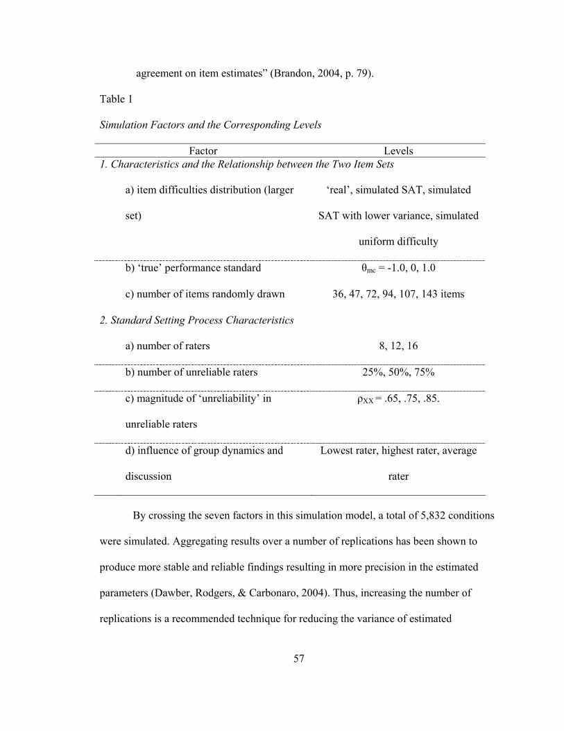
57
agreement on item estimates” (Brandon, 2004, p. 79).
Table 1
Simulation Factors and the Corresponding Levels
Factor Levels 1. Characteristics and the Relationship between the Two Item Sets
a) item difficulties distribution (larger
set)
‘real’, simulated SAT, simulated
SAT with lower variance, simulated
uniform difficulty
b) ‘true’ performance standard θmc = -1.0, 0, 1.0
c) number of items randomly drawn 36, 47, 72, 94, 107, 143 items
2. Standard Setting Process Characteristics
a) number of raters 8, 12, 16
b) number of unreliable raters 25%, 50%, 75%
c) magnitude of ‘unreliability’ in
unreliable raters
ρXX = .65, .75, .85.
d) influence of group dynamics and
discussion
Lowest rater, highest rater, average
rater
By crossing the seven factors in this simulation model, a total of 5,832 conditions
were simulated. Aggregating results over a number of replications has been shown to
produce more stable and reliable findings resulting in more precision in the estimated
parameters (Dawber, Rodgers, & Carbonaro, 2004). Thus, increasing the number of
replications is a recommended technique for reducing the variance of estimated
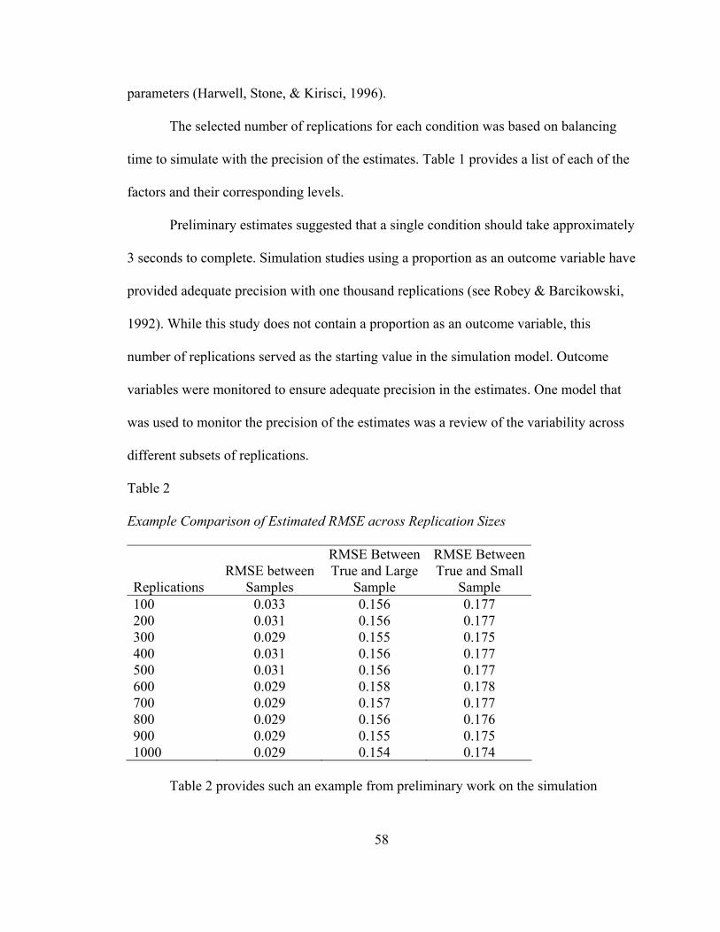
58
parameters (Harwell, Stone, & Kirisci, 1996).
The selected number of replications for each condition was based on balancing
time to simulate with the precision of the estimates. Table 1 provides a list of each of the
factors and their corresponding levels.
Preliminary estimates suggested that a single condition should take approximately
3 seconds to complete. Simulation studies using a proportion as an outcome variable have
provided adequate precision with one thousand replications (see Robey & Barcikowski,
1992). While this study does not contain a proportion as an outcome variable, this
number of replications served as the starting value in the simulation model. Outcome
variables were monitored to ensure adequate precision in the estimates. One model that
was used to monitor the precision of the estimates was a review of the variability across
different subsets of replications.
Table 2
Example Comparison of Estimated RMSE across Replication Sizes
Replications RMSE between
Samples
RMSE Between True and Large
Sample
RMSE Between True and Small
Sample 100 0.033 0.156 0.177 200 0.031 0.156 0.177 300 0.029 0.155 0.175 400 0.031 0.156 0.177 500 0.031 0.156 0.177 600 0.029 0.158 0.178 700 0.029 0.157 0.177 800 0.029 0.156 0.176 900 0.029 0.155 0.175 1000 0.029 0.154 0.174
Table 2 provides such an example from preliminary work on the simulation
59
model. The outcome variables such as the estimated root mean squared error (RMSE)
was compared across different sets of replications, 100 to 1,000 in increments of 100 in
this example. This change in the RMSE estimates across the different sets of replications
can be used to determine whether an appropriate level of precision has been achieved in
the estimates. For example, the estimated RMSE ‘across’ the two samples results in no
change (three decimal places) from 600 through 1,000 replications. The change in the
estimated RMSE for the other comparisons (between true and large; between true and
small) shows a difference of 0.004 over the same sets of replication sizes. Based on the
number of conditions and the 1,000 replications for each condition, the total number of
simulations was 5,832,000.
The original estimate was that the full simulation would take 3,037.5 hours of
computer time or roughly 31.6 days to complete the simulations using three computers
running non-stop 24 hours per day. This original estimate was very close to the actual
time it took to run the simulations.
Simulation Procedures
Figure 1 displays a flowchart containing each phase of the simulation process,
including the two rounds involved in data generation, the creation of the datasets, and the
evaluation of the results. In addition to the phases in the simulation process, the
simulation constants and various design factors points in the process are noted as well.
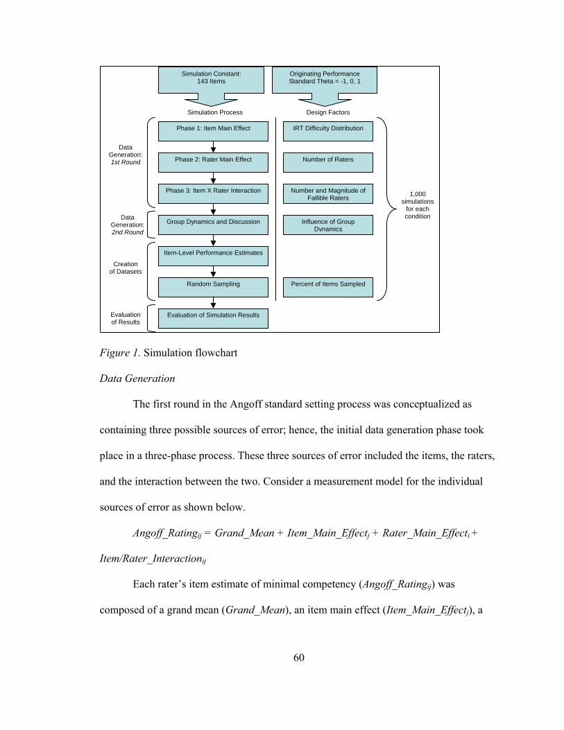
60
Figure 1. Simulation flowchart
Data Generation
The first round in the Angoff standard setting process was conceptualized as
containing three possible sources of error; hence, the initial data generation phase took
place in a three-phase process. These three sources of error included the items, the raters,
and the interaction between the two. Consider a measurement model for the individual
sources of error as shown below.
Angoff_Ratingij = Grand_Mean + Item_Main_Effectj + Rater_Main_Effecti +
Item/Rater_Interactionij
Each rater’s item estimate of minimal competency (Angoff_Ratingij) was
composed of a grand mean (Grand_Mean), an item main effect (Item_Main_Effectj), a
Phase 1: Item Main Effect
Phase 2: Rater Main Effect
Phase 3: Item X Rater Interaction
Data Generation: 1st Round
Group Dynamics and Discussion
Evaluation of Simulation Results
Item-Level Performance Estimates
1,000 simulations
for each condition Data
Generation: 2nd Round
Random Sampling
Creation of Datasets
Evaluation of Results
IRT Difficulty Distribution
Number of Raters
Number and Magnitude of Fallible Raters
Influence of Group Dynamics
Percent of Items Sampled
Simulation Process Design Factors
Simulation Constant: 143 Items
Originating Performance Standard Theta = -1, 0, 1
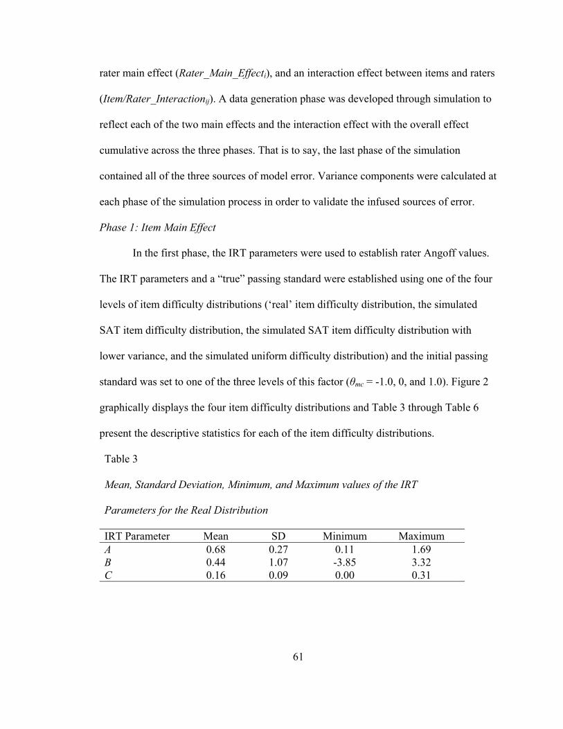
61
rater main effect (Rater_Main_Effecti), and an interaction effect between items and raters
(Item/Rater_Interactionij). A data generation phase was developed through simulation to
reflect each of the two main effects and the interaction effect with the overall effect
cumulative across the three phases. That is to say, the last phase of the simulation
contained all of the three sources of model error. Variance components were calculated at
each phase of the simulation process in order to validate the infused sources of error.
Phase 1: Item Main Effect
In the first phase, the IRT parameters were used to establish rater Angoff values.
The IRT parameters and a “true” passing standard were established using one of the four
levels of item difficulty distributions (‘real’ item difficulty distribution, the simulated
SAT item difficulty distribution, the simulated SAT item difficulty distribution with
lower variance, and the simulated uniform difficulty distribution) and the initial passing
standard was set to one of the three levels of this factor (θmc = -1.0, 0, and 1.0). Figure 2
graphically displays the four item difficulty distributions and Table 3 through Table 6
present the descriptive statistics for each of the item difficulty distributions.
Table 3
Mean, Standard Deviation, Minimum, and Maximum values of the IRT
Parameters for the Real Distribution
IRT Parameter Mean SD Minimum Maximum A 0.68 0.27 0.11 1.69 B 0.44 1.07 -3.85 3.32 C 0.16 0.09 0.00 0.31
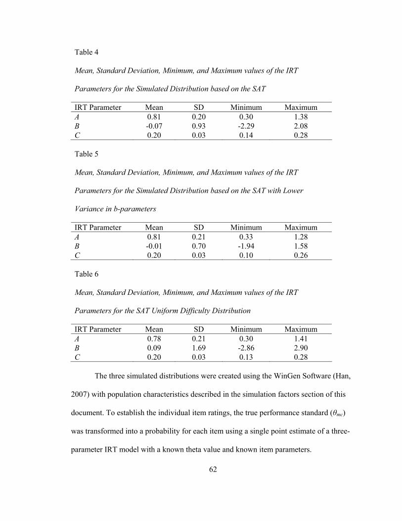
62
Table 4
Mean, Standard Deviation, Minimum, and Maximum values of the IRT
Parameters for the Simulated Distribution based on the SAT
IRT Parameter Mean SD Minimum Maximum A 0.81 0.20 0.30 1.38 B -0.07 0.93 -2.29 2.08 C 0.20 0.03 0.14 0.28
Table 5
Mean, Standard Deviation, Minimum, and Maximum values of the IRT
Parameters for the Simulated Distribution based on the SAT with Lower
Variance in b-parameters
IRT Parameter Mean SD Minimum Maximum A 0.81 0.21 0.33 1.28 B -0.01 0.70 -1.94 1.58 C 0.20 0.03 0.10 0.26
Table 6
Mean, Standard Deviation, Minimum, and Maximum values of the IRT
Parameters for the SAT Uniform Difficulty Distribution
IRT Parameter Mean SD Minimum Maximum A 0.78 0.21 0.30 1.41 B 0.09 1.69 -2.86 2.90 C 0.20 0.03 0.13 0.28
The three simulated distributions were created using the WinGen Software (Han,
2007) with population characteristics described in the simulation factors section of this
document. To establish the individual item ratings, the true performance standard (θmc)
was transformed into a probability for each item using a single point estimate of a three-
parameter IRT model with a known theta value and known item parameters.
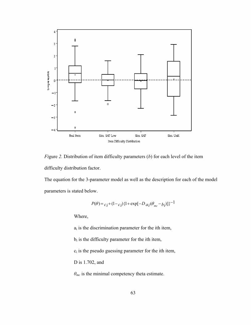
63
Figure 2. Distribution of item difficulty parameters (b) for each level of the item
difficulty distribution factor.
The equation for the 3-parameter model as well as the description for each of the model
parameters is stated below.
1)]}(exp[1){1()( −−−+−+= biaiDciciP mcθθ
Where,
ai is the discrimination parameter for the ith item,
bi is the difficulty parameter for the ith item,
ci is the pseudo guessing parameter for the ith item,
D is 1.702, and
θmc is the minimal competency theta estimate.
64
The three IRT parameters in the model are further described as follows: (1) the a-
parameter is the discrimination index of the item, (2) the b-parameter is the difficulty of
the item and, (3) the c-parameter is the index of the pseudo guessing parameter for the
item.
The derived probability, p(θ), was then averaged across all items and this value
represented the grand mean (Grand_Mean) in the model. To establish the individual
items means, the grand mean was subtracted from the overall item effect. The scale of the
Angoff ratings was then changed to reflect practice (multiplied by 100). Raters are
normally instructed to contemplate 100 minimally competent examinees and determine
the number out of a hundred that would correctly respond to the item as opposed to
determining a probability of success.
An example has been constructed to demonstrate the changes to the data structure
through each phase in the simulation process. Each phase will be displayed as a table
displaying six items with their corresponding item IRT parameters items, simulated
Angoff values, estimated item-level theta performance estimates ( imcθ̂ ) as well as the
estimated overall theta performance estimate for the six-item set ( kmcθ̂ ). The estimated
overall theta performance estimate for the six items, kmcθ̂ , is the mean imcθ̂ across items.
The calculation of the item level performance estimates, imcθ̂ , will be discussed later in
this section. For example purposes, the originating theta in the sample tables will be 0
and the calculated grand mean is 0.476.
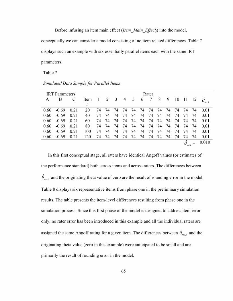
65
Before infusing an item main effect (Item_Main_Effectj) into the model,
conceptually we can consider a model consisting of no item related differences. Table 7
displays such an example with six essentially parallel items each with the same IRT
parameters.
Table 7
Simulated Data Sample for Parallel Items
IRT Parameters Rater A B C Item
# 1 2 3 4 5 6 7 8 9 10 11 12
imcθ̂
0.60 -0.69 0.21 20 74 74 74 74 74 74 74 74 74 74 74 74 0.01 0.60 -0.69 0.21 40 74 74 74 74 74 74 74 74 74 74 74 74 0.01 0.60 -0.69 0.21 60 74 74 74 74 74 74 74 74 74 74 74 74 0.01 0.60 -0.69 0.21 80 74 74 74 74 74 74 74 74 74 74 74 74 0.01 0.60 -0.69 0.21 100 74 74 74 74 74 74 74 74 74 74 74 74 0.01 0.60 -0.69 0.21 120 74 74 74 74 74 74 74 74 74 74 74 74 0.01
kmcθ̂ = 0.010
In this first conceptual stage, all raters have identical Angoff values (or estimates of
the performance standard) both across items and across raters. The differences between
kmcθ̂ and the originating theta value of zero are the result of rounding error in the model.
Table 8 displays six representative items from phase one in the preliminary simulation
results. The table presents the item-level differences resulting from phase one in the
simulation process. Since this first phase of the model is designed to address item error
only, no rater error has been introduced in this example and all the individual raters are
assigned the same Angoff rating for a given item. The differences between kmcθ̂ and the
originating theta value (zero in this example) were anticipated to be small and are
primarily the result of rounding error in the model.
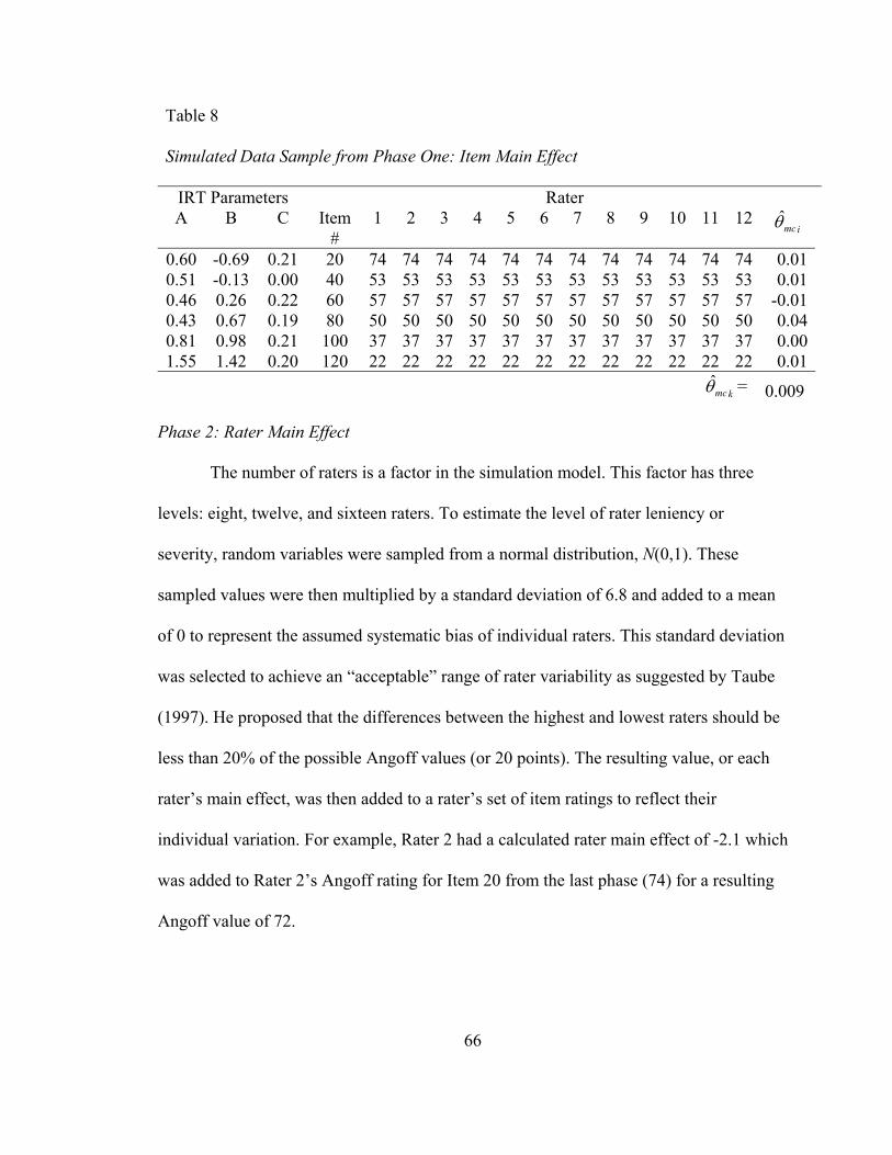
66
Table 8
Simulated Data Sample from Phase One: Item Main Effect
IRT Parameters Rater A B C Item
# 1 2 3 4 5 6 7 8 9 10 11 12
imcθ̂
0.60 -0.69 0.21 20 74 74 74 74 74 74 74 74 74 74 74 74 0.010.51 -0.13 0.00 40 53 53 53 53 53 53 53 53 53 53 53 53 0.010.46 0.26 0.22 60 57 57 57 57 57 57 57 57 57 57 57 57 -0.010.43 0.67 0.19 80 50 50 50 50 50 50 50 50 50 50 50 50 0.040.81 0.98 0.21 100 37 37 37 37 37 37 37 37 37 37 37 37 0.001.55 1.42 0.20 120 22 22 22 22 22 22 22 22 22 22 22 22 0.01
kmcθ̂ = 0.009
Phase 2: Rater Main Effect
The number of raters is a factor in the simulation model. This factor has three
levels: eight, twelve, and sixteen raters. To estimate the level of rater leniency or
severity, random variables were sampled from a normal distribution, N(0,1). These
sampled values were then multiplied by a standard deviation of 6.8 and added to a mean
of 0 to represent the assumed systematic bias of individual raters. This standard deviation
was selected to achieve an “acceptable” range of rater variability as suggested by Taube
(1997). He proposed that the differences between the highest and lowest raters should be
less than 20% of the possible Angoff values (or 20 points). The resulting value, or each
rater’s main effect, was then added to a rater’s set of item ratings to reflect their
individual variation. For example, Rater 2 had a calculated rater main effect of -2.1 which
was added to Rater 2’s Angoff rating for Item 20 from the last phase (74) for a resulting
Angoff value of 72.
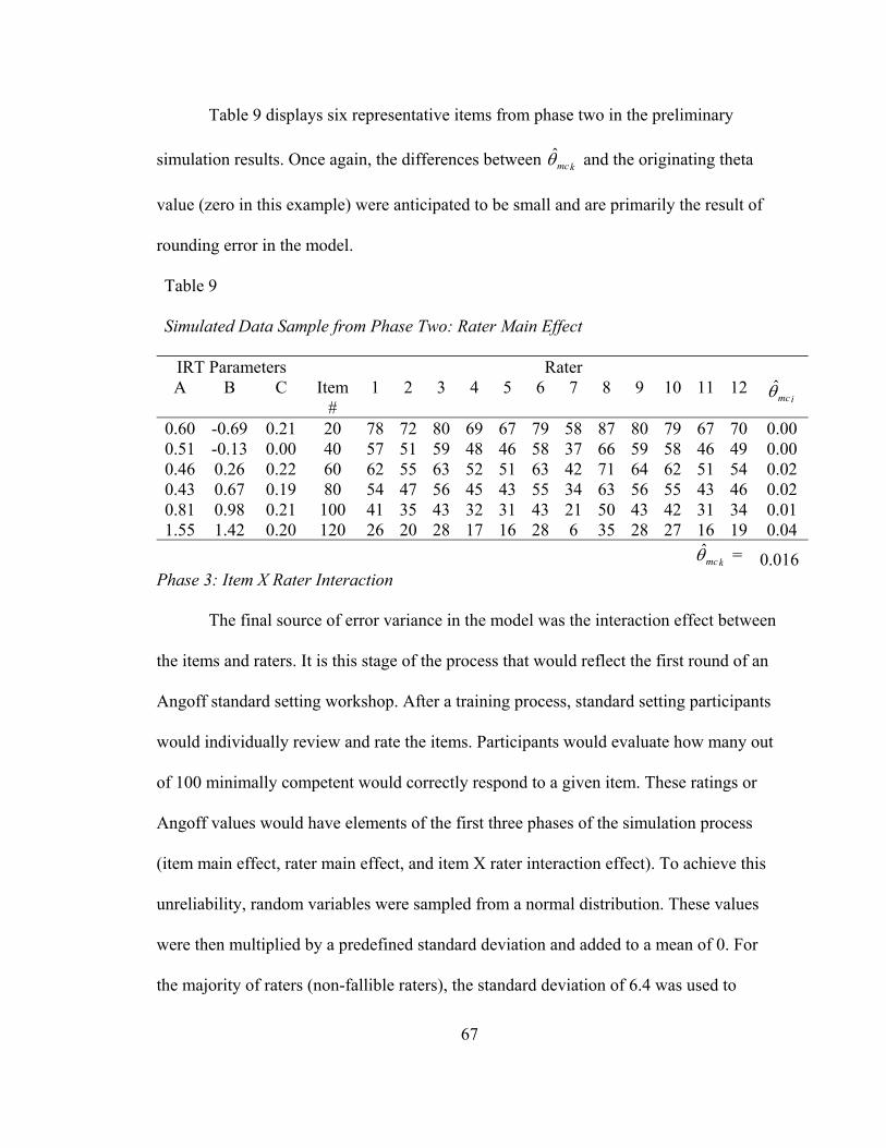
67
Table 9 displays six representative items from phase two in the preliminary
simulation results. Once again, the differences between kmcθ̂ and the originating theta
value (zero in this example) were anticipated to be small and are primarily the result of
rounding error in the model.
Table 9
Simulated Data Sample from Phase Two: Rater Main Effect
IRT Parameters Rater A B C Item
# 1 2 3 4 5 6 7 8 9 10 11 12
imcθ̂
0.60 -0.69 0.21 20 78 72 80 69 67 79 58 87 80 79 67 70 0.00 0.51 -0.13 0.00 40 57 51 59 48 46 58 37 66 59 58 46 49 0.00 0.46 0.26 0.22 60 62 55 63 52 51 63 42 71 64 62 51 54 0.02 0.43 0.67 0.19 80 54 47 56 45 43 55 34 63 56 55 43 46 0.02 0.81 0.98 0.21 100 41 35 43 32 31 43 21 50 43 42 31 34 0.01 1.55 1.42 0.20 120 26 20 28 17 16 28 6 35 28 27 16 19 0.04
kmcθ̂ = 0.016
Phase 3: Item X Rater Interaction
The final source of error variance in the model was the interaction effect between
the items and raters. It is this stage of the process that would reflect the first round of an
Angoff standard setting workshop. After a training process, standard setting participants
would individually review and rate the items. Participants would evaluate how many out
of 100 minimally competent would correctly respond to a given item. These ratings or
Angoff values would have elements of the first three phases of the simulation process
(item main effect, rater main effect, and item X rater interaction effect). To achieve this
unreliability, random variables were sampled from a normal distribution. These values
were then multiplied by a predefined standard deviation and added to a mean of 0. For
the majority of raters (non-fallible raters), the standard deviation of 6.4 was used to
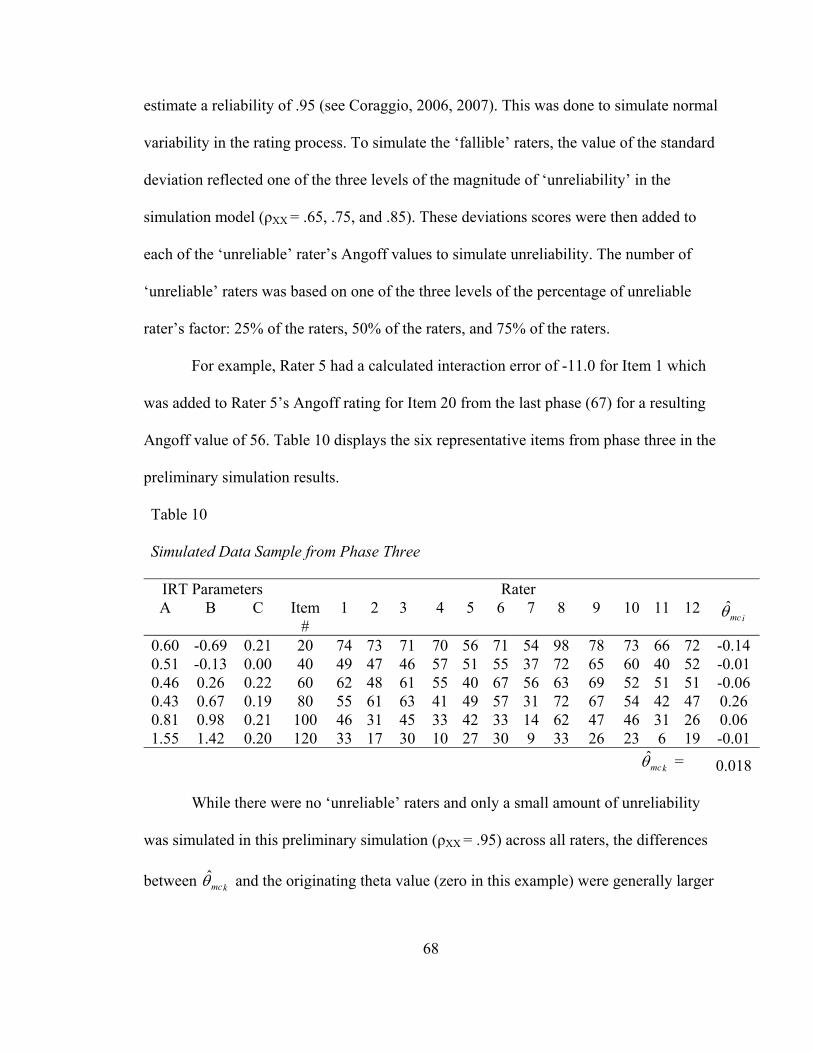
68
estimate a reliability of .95 (see Coraggio, 2006, 2007). This was done to simulate normal
variability in the rating process. To simulate the ‘fallible’ raters, the value of the standard
deviation reflected one of the three levels of the magnitude of ‘unreliability’ in the
simulation model (ρXX = .65, .75, and .85). These deviations scores were then added to
each of the ‘unreliable’ rater’s Angoff values to simulate unreliability. The number of
‘unreliable’ raters was based on one of the three levels of the percentage of unreliable
rater’s factor: 25% of the raters, 50% of the raters, and 75% of the raters.
For example, Rater 5 had a calculated interaction error of -11.0 for Item 1 which
was added to Rater 5’s Angoff rating for Item 20 from the last phase (67) for a resulting
Angoff value of 56. Table 10 displays the six representative items from phase three in the
preliminary simulation results.
Table 10
Simulated Data Sample from Phase Three
IRT Parameters Rater A B C Item
# 1 2 3 4 5 6 7 8 9 10 11 12
imcθ̂
0.60 -0.69 0.21 20 74 73 71 70 56 71 54 98 78 73 66 72 -0.14 0.51 -0.13 0.00 40 49 47 46 57 51 55 37 72 65 60 40 52 -0.01 0.46 0.26 0.22 60 62 48 61 55 40 67 56 63 69 52 51 51 -0.06 0.43 0.67 0.19 80 55 61 63 41 49 57 31 72 67 54 42 47 0.26 0.81 0.98 0.21 100 46 31 45 33 42 33 14 62 47 46 31 26 0.06 1.55 1.42 0.20 120 33 17 30 10 27 30 9 33 26 23 6 19 -0.01
kmcθ̂ = 0.018
While there were no ‘unreliable’ raters and only a small amount of unreliability
was simulated in this preliminary simulation (ρXX = .95) across all raters, the differences
between kmcθ̂ and the originating theta value (zero in this example) were generally larger
69
at this phase depending on the number of ‘unreliable’ raters and the magnitude of their
unreliability. Even in this preliminary simulation, however, differences as a result of the
unreliability can be seen for specific items such as Item 80. This is largely due to the
restricted number of raters and items in the simulation model.
Group Dynamics and Discussion
After the conditions for the initial standard setting round was complete, the
second round or discussion round was simulated. The discussion round of the Angoff
standard setting workshop usually includes a group discussion regarding those items that
did not meet some predetermined level of group consensus. This process usually involves
an item-by-item review of those highlighted items with a statement from the highest and
the lowest rater regarding their justifications for their individual ratings. Other
participants generally add to the discussion as well. Finally, standard setting participants
are asked to review their individual ratings for a given item and are permitted to change
their ratings if they so choose. Standard setting research on second round performance
suggests that providing information to raters will generally produce “small and
inconsistent” changes in the overall mean performance standard, but will result in lower
rater variability (Busch & Jaeger, 1990, p. 148). Brandon (2004) after conducting a
review of the empirical literature on modified Angoff standard setting also concluded that
the variability of rater estimates decreases after raters engage in between-round activities.
Researchers have also suggested a group-influenced biasing effect of regression to the
mean (Livingston, 1995) in addition to a group polarization effect during the discussion
phase (Fitzpatrick, 1989). To address the uniform rating regression and the directional
70
influence of dominant raters, individual rater performance estimates were adjusted
directionally based on one of the three levels of the influence factor: the lowest rater
influence, the highest rater influence, and the average rater influence. The following
formula based on an adjustment proposed by Reckase (2006b) was used to simulate this
group influence during the discussion phase of the standard setting process:
rating = ε + (rating - ε) * influence_factor
Where, ε is the rating of the influencing rater (lowest rater, the highest rater, or
the average rater) as mentioned in the three levels of the influence factor, and the rating
represents the individual item rating of the standard setting participant. To estimate the
level of variability for the rater’s level of influence, an influence_factor was calculated
using random variables sampled from a normal distribution, N(0,1). These sampled
values were then multiplied by a standard deviation of 0.1 and added to a mean of 0.7.
These values were selected to provide an acceptable amount of variability in the degree
of influence for each rater. This influence_factor was assigned to each individual rater
and used systematically in each of their item ratings for the discussion phase of the
simulation.
For example, the average rater was the level of the directional influence for the
preliminary simulation and the mean rating for Item 1 was 70.67. Rater 7 had a
calculated influence_factor of 0.84 and a rating for Item 1 of 54. The resulting calculation
was 70.67 + (54 -70.67) * 0.84 or 57. Table 11 displays six representative items from the
discussion phase in the preliminary simulation results. While there was little difference
between the kmcθ̂ calculated in the third phase and the kmcθ̂ calculated in the discussion
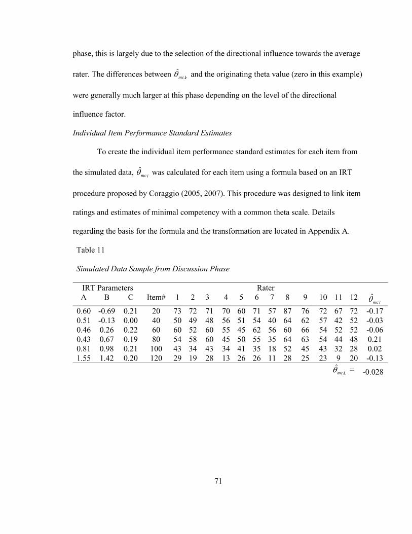
71
phase, this is largely due to the selection of the directional influence towards the average
rater. The differences between kmcθ̂ and the originating theta value (zero in this example)
were generally much larger at this phase depending on the level of the directional
influence factor.
Individual Item Performance Standard Estimates
To create the individual item performance standard estimates for each item from
the simulated data, imcθ̂ was calculated for each item using a formula based on an IRT
procedure proposed by Coraggio (2005, 2007). This procedure was designed to link item
ratings and estimates of minimal competency with a common theta scale. Details
regarding the basis for the formula and the transformation are located in Appendix A.
Table 11
Simulated Data Sample from Discussion Phase
IRT Parameters Rater A B C Item# 1 2 3 4 5 6 7 8 9 10 11 12
imcθ̂ 0.60 -0.69 0.21 20 73 72 71 70 60 71 57 87 76 72 67 72 -0.17 0.51 -0.13 0.00 40 50 49 48 56 51 54 40 64 62 57 42 52 -0.03 0.46 0.26 0.22 60 60 52 60 55 45 62 56 60 66 54 52 52 -0.06 0.43 0.67 0.19 80 54 58 60 45 50 55 35 64 63 54 44 48 0.21 0.81 0.98 0.21 100 43 34 43 34 41 35 18 52 45 43 32 28 0.02 1.55 1.42 0.20 120 29 19 28 13 26 26 11 28 25 23 9 20 -0.13
kmcθ̂ = -0.028
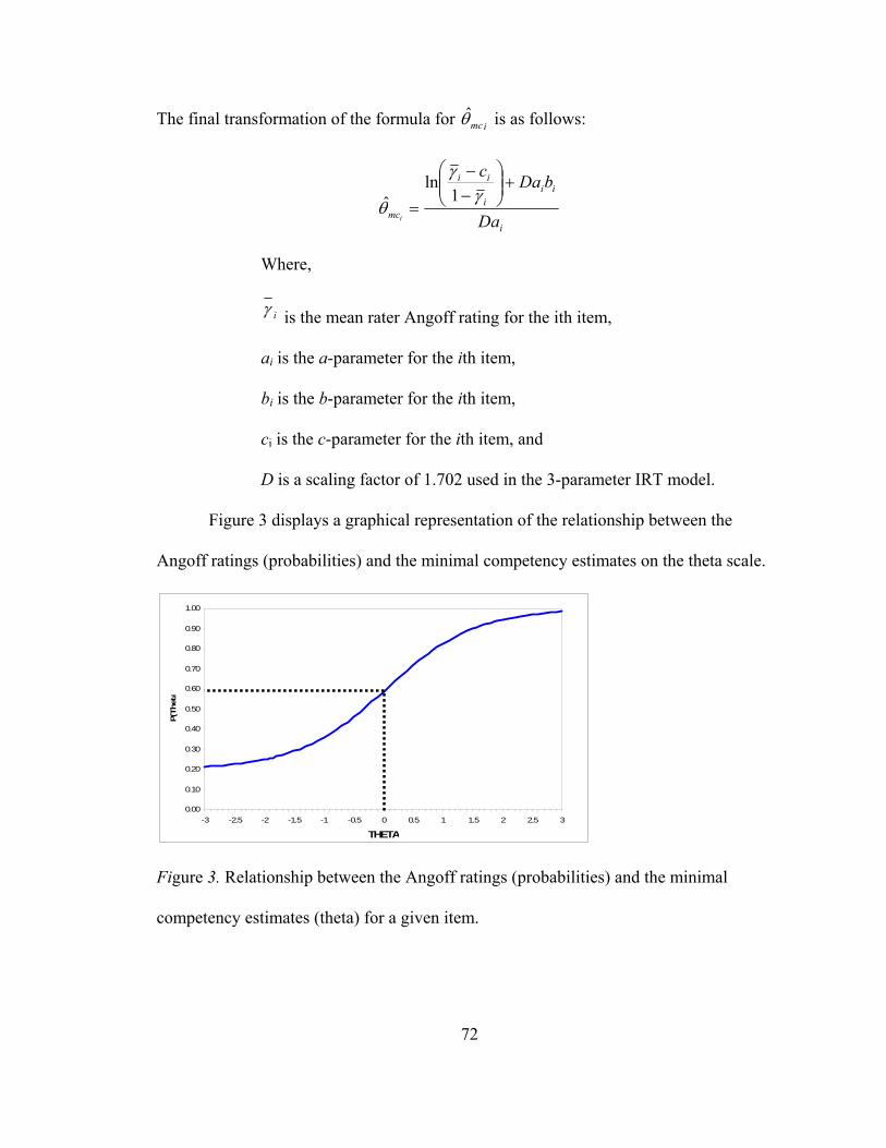
72
The final transformation of the formula for imcθ̂ is as follows:
i
iii
ii
mc Da
bDac
i
+⎟⎟⎠
⎞⎜⎜⎝
⎛−−
=γ
γ
θ1
lnˆ
Where,
iγ is the mean rater Angoff rating for the ith item,
ai is the a-parameter for the ith item,
bi is the b-parameter for the ith item,
ci is the c-parameter for the ith item, and
D is a scaling factor of 1.702 used in the 3-parameter IRT model.
Figure 3 displays a graphical representation of the relationship between the
Angoff ratings (probabilities) and the minimal competency estimates on the theta scale.
0.00
0.10
0.20
0.30
0.40
0.50
0.60
0.70
0.80
0.90
1.00
-3 -2.5 -2 -1.5 -1 -0.5 0 0.5 1 1.5 2 2.5 3
THETA
P(Th
eta
Figure 3. Relationship between the Angoff ratings (probabilities) and the minimal
competency estimates (theta) for a given item.
73
The simulation program produced 143 item-level performance standard estimates
( imcθ̂ ). A sampling macro, samplethetas2, was run to perform stratified random sampling
on the full 143-item dataset. A stratified sampling model was designed to create a sample
that was similar in terms of item difficulty and item discrimination as the original 143-
item set. This model is consistent with the current literature in item selection strategies
for standard setting. Ferdous and Plake (2007) used a similar sampling method that
stratified samples according to content, item p-values, and item discrimination levels.
Smith and Ferdous (2007) found that sampling models that stratified on p-value intervals
and p-value density assist in reducing the standard error of the cutscore. The previous
methods have predominately used classical statistics with pre-existing datasets in
employing their stratified sampling models. This study sought to build on this previous
research by employing a sampling model that stratified on item difficulty (b-parameters)
and item discrimination (a-parameters).
Item difficulty distributions were separated into thirds by item difficulty and item
discrimination parameters. A three-by-three stratification matrix was then constructed for
each individual item difficulty distribution. The corresponding percentages of items in
each cell were used along with the surveyselect procedure in SAS to create the individual
samples. This ensured that the samples were similar to the full 143-item set in terms of
item difficulty and item discrimination. The size of the sample varied depending on the
level of the factor. The number of items sampled was 36, 47, 72, 94, and 107. The sample
sizes represented approximately 25%, 33%, 50%, 66%, and 75% of the total number of
items. The full 143-item set was also included as a comparison group. The difference
74
between the sample performance estimate, the performance estimate derived from the
complete 143 item set, and the ‘true’ originating performance estimate was stored and
aggregated across the simulations. Appendix B contains the SAS code for one set of
conditions from the generalizability study.
Simulation Model Validation
The first criticism of any simulation procedure is whether the results can be
generalized to ‘real life’ situations. Without any real life generalizability, the results of
the simulation study add little or no contribution to the body of research literature. The
ideal approach is to begin with a simulation model that has already been validated
through previous research. Unfortunately, little research exists in the area of standard
setting simulation studies and the basis for this proposed simulation model has only
recently been explored. In order to begin to establish the validity of this proposed
simulation process, multiple sources of internal and external validity evidence are
presented below. While individually each source may not provide enough evidence to
validate the model on its own merit, cumulatively they begin to provide a solid basis of
support.
Internal Sources of Validity Evidence
Sources of Error. To validate the sources of error in the model (item, rater, and
item/rater interaction), variance components were used to verify that error was
appropriately applied to the originating source. These variance components were
calculated as an element of the simulation process and were periodically reviewed during
preliminary simulations to ensure that the process was operating as intended.
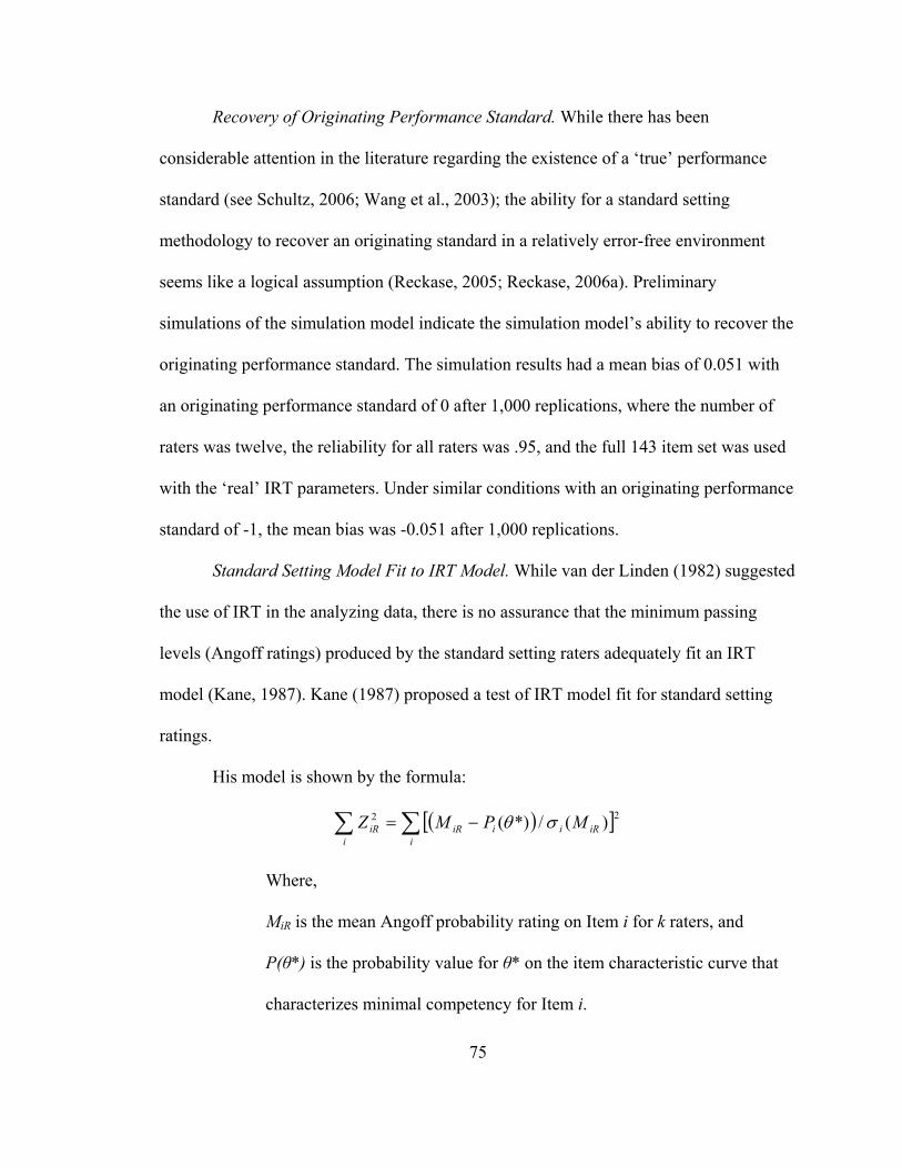
75
Recovery of Originating Performance Standard. While there has been
considerable attention in the literature regarding the existence of a ‘true’ performance
standard (see Schultz, 2006; Wang et al., 2003); the ability for a standard setting
methodology to recover an originating standard in a relatively error-free environment
seems like a logical assumption (Reckase, 2005; Reckase, 2006a). Preliminary
simulations of the simulation model indicate the simulation model’s ability to recover the
originating performance standard. The simulation results had a mean bias of 0.051 with
an originating performance standard of 0 after 1,000 replications, where the number of
raters was twelve, the reliability for all raters was .95, and the full 143 item set was used
with the ‘real’ IRT parameters. Under similar conditions with an originating performance
standard of -1, the mean bias was -0.051 after 1,000 replications.
Standard Setting Model Fit to IRT Model. While van der Linden (1982) suggested
the use of IRT in the analyzing data, there is no assurance that the minimum passing
levels (Angoff ratings) produced by the standard setting raters adequately fit an IRT
model (Kane, 1987). Kane (1987) proposed a test of IRT model fit for standard setting
ratings.
His model is shown by the formula:
( )[ ]∑ ∑ −=i i
iRiiiRiR MPMZ 22 )(/*)( σθ
Where,
MiR is the mean Angoff probability rating on Item i for k raters, and
P(θ*) is the probability value for θ* on the item characteristic curve that
characterizes minimal competency for Item i.
76
The resulting value is distributed as a chi-square with n -1 degrees of freedom.
While Kane (1987) did not provide an example using actual data, he did suggest that the
issue of independence could be “problematic when all items are reviewed by the same
raters” (p. 336). He felt that the independence assumption should be robust as long as the
correlated errors are small compared to the random errors, specifically, the variation in
specific raters rating specific items over different occasions. Preliminary simulation
results were evaluated using Kane’s IRT fit model. Results suggest that these standard
setting data correctly fit an IRT framework. This result is not completely unexpected as
IRT was used to initially determine the estimates, however, it does provide additional
validation evidence for the simulation model.
External Sources of Validity Evidence
Research Basis for Simulation Factors and Corresponding Levels. When
possible, each factor and its associated levels were related to actual standard setting
conditions as discussed earlier in the simulation factors section of this document. For
example, the ‘real’ IRT parameters were previously published parameters and the other
simulated distributions were established from published information on the SAT
examination. Other examples include the number of raters and the influence of group
dynamics conditions.
Similarity of Simulation Data Characteristics with Performance Data in the
Literature. Simulation data characteristics were similar to those presented in the research
literature. For example, the variance in rater estimates decreased between the first and
second round while little change occurred in overall performance standard estimate. This
77
finding is consistent with published research (Busch & Jaeger, 1990; Hurtz & Auerbach,
2003).
Review by Content Expert. A preliminary study using a similar version of the
simulation model (Coraggio, 2007) was reviewed by a notable expert in the area of
standard setting and generalizing performance standards, his comments regarding the
methodology were very favorable with no suggested changes to the simulation
methodology (S. G. Sireci, personal interview, April 11, 2007).
Comparisons to ‘Real’ Standard Setting Datasets. The availability of Angoff
datasets is limited in the existing research for reasons of privacy and test security. For
purposes of model validity, comparisons were made between an actual two round Angoff
dataset (provided by S. G. Sireci) and simulated dataset with similar characteristics. The
actual Angoff dataset contained 13 raters. One rater was randomly selected and removed
in order to match simulation parameters.
Comparisons were made between the phase 3 of the simulation (item X rater
interaction phase) and the initial round (independent ratings) of the actual Angoff dataset.
Since the simulation was designed to represent a number of factors across various
conditions, research was conducted to find the condition which had the closest
representation to the actual Angoff dataset. Due to the nature of simulation study,
individual conditions contained replication results which had a certain amount of
variability. Therefore, multiple replications were also simulated for conditions which
produced similar results.
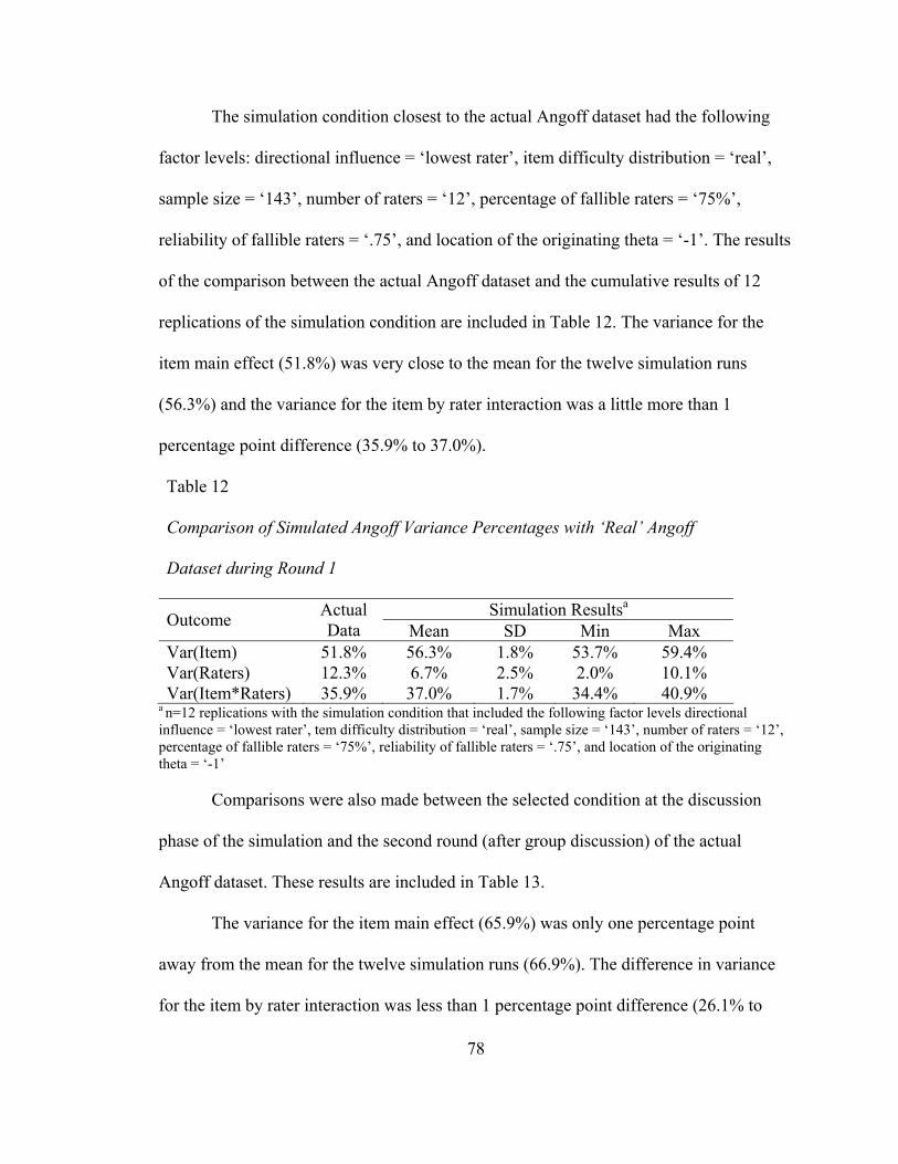
78
The simulation condition closest to the actual Angoff dataset had the following
factor levels: directional influence = ‘lowest rater’, item difficulty distribution = ‘real’,
sample size = ‘143’, number of raters = ‘12’, percentage of fallible raters = ‘75%’,
reliability of fallible raters = ‘.75’, and location of the originating theta = ‘-1’. The results
of the comparison between the actual Angoff dataset and the cumulative results of 12
replications of the simulation condition are included in Table 12. The variance for the
item main effect (51.8%) was very close to the mean for the twelve simulation runs
(56.3%) and the variance for the item by rater interaction was a little more than 1
percentage point difference (35.9% to 37.0%).
Table 12
Comparison of Simulated Angoff Variance Percentages with ‘Real’ Angoff
Dataset during Round 1
Simulation Resultsa Outcome Actual Data Mean SD Min Max
Var(Item) 51.8% 56.3% 1.8% 53.7% 59.4% Var(Raters) 12.3% 6.7% 2.5% 2.0% 10.1% Var(Item*Raters) 35.9% 37.0% 1.7% 34.4% 40.9%
a n=12 replications with the simulation condition that included the following factor levels directional influence = ‘lowest rater’, tem difficulty distribution = ‘real’, sample size = ‘143’, number of raters = ‘12’, percentage of fallible raters = ‘75%’, reliability of fallible raters = ‘.75’, and location of the originating theta = ‘-1’ Comparisons were also made between the selected condition at the discussion
phase of the simulation and the second round (after group discussion) of the actual
Angoff dataset. These results are included in Table 13.
The variance for the item main effect (65.9%) was only one percentage point
away from the mean for the twelve simulation runs (66.9%). The difference in variance
for the item by rater interaction was less than 1 percentage point difference (26.1% to
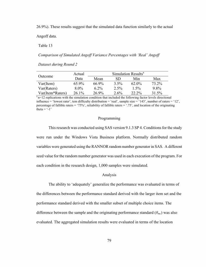
79
26.9%). These results suggest that the simulated data function similarly to the actual
Angoff data.
Table 13
Comparison of Simulated Angoff Variance Percentages with ‘Real’ Angoff
Dataset during Round 2
Simulation Resultsa Outcome Actual Data Mean SD Min Max
Var(Item) 65.9% 66.9% 3.5% 62.0% 73.2% Var(Raters) 8.0% 6.2% 2.5% 1.5% 9.8% Var(Item*Raters) 26.1% 26.9% 2.6% 22.2% 31.5%
a n=12 replications with the simulation condition that included the following factor levels directional influence = ‘lowest rater’, tem difficulty distribution = ‘real’, sample size = ‘143’, number of raters = ‘12’, percentage of fallible raters = ‘75%’, reliability of fallible raters = ‘.75’, and location of the originating theta = ‘-1’
Programming
This research was conducted using SAS version 9.1.3 SP 4. Conditions for the study
were run under the Windows Vista Business platform. Normally distributed random
variables were generated using the RANNOR random number generator in SAS. A different
seed value for the random number generator was used in each execution of the program. For
each condition in the research design, 1,000 samples were simulated.
Analysis
The ability to ‘adequately’ generalize the performance was evaluated in terms of
the differences between the performance standard derived with the larger item set and the
performance standard derived with the smaller subset of multiple choice items. The
difference between the sample and the originating performance standard (θmc) was also
evaluated. The aggregated simulation results were evaluated in terms of the location
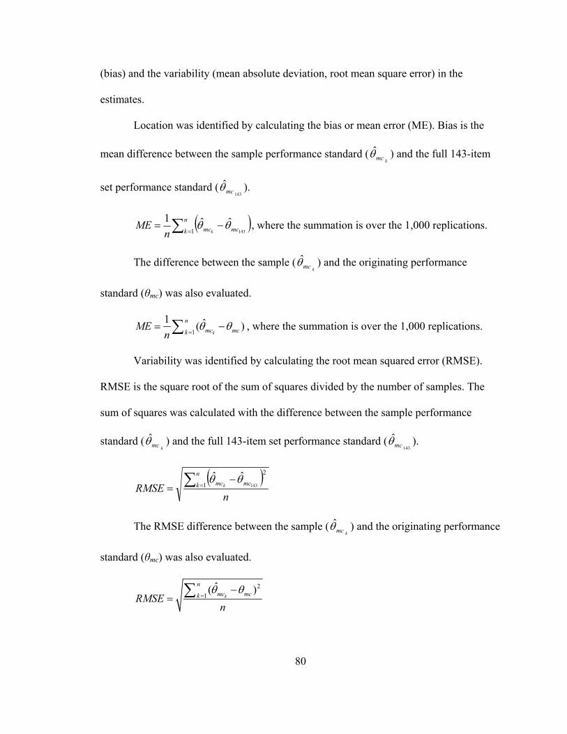
80
(bias) and the variability (mean absolute deviation, root mean square error) in the
estimates.
Location was identified by calculating the bias or mean error (ME). Bias is the
mean difference between the sample performance standard (kmcθ̂ ) and the full 143-item
set performance standard (143
ˆmcθ ).
( )∑ =−=
n
k mcmcknME
1 143ˆˆ1 θθ , where the summation is over the 1,000 replications.
The difference between the sample (kmcθ̂ ) and the originating performance
standard (θmc) was also evaluated.
1
1 ˆ( )k
nmc mck
MEn
θ θ=
= −∑ , where the summation is over the 1,000 replications.
Variability was identified by calculating the root mean squared error (RMSE).
RMSE is the square root of the sum of squares divided by the number of samples. The
sum of squares was calculated with the difference between the sample performance
standard (kmcθ̂ ) and the full 143-item set performance standard (
143
ˆmcθ ).
( )n
RMSEn
k mcmck∑ =−
= 1
2
143ˆˆ θθ
The RMSE difference between the sample (kmcθ̂ ) and the originating performance
standard (θmc) was also evaluated.
21
ˆ( )k
nmc mckRMSEn
θ θ=
−= ∑
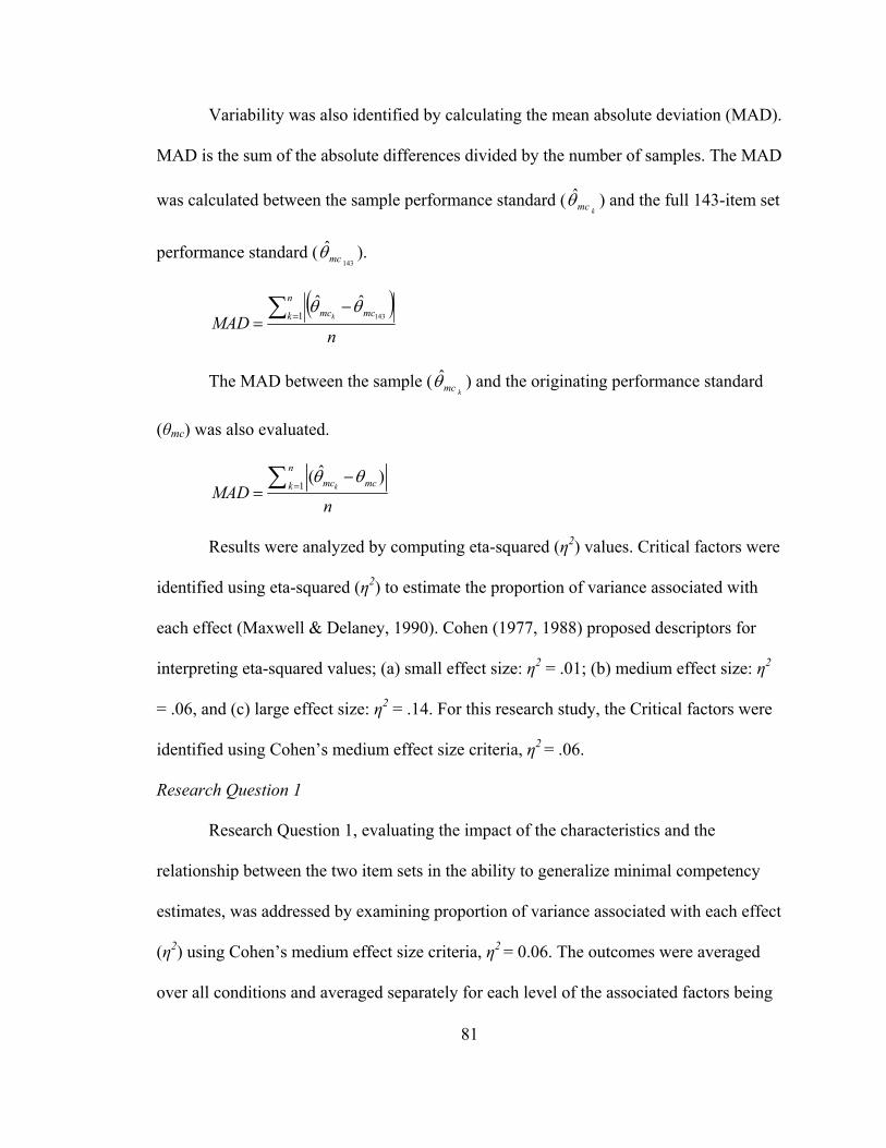
81
Variability was also identified by calculating the mean absolute deviation (MAD).
MAD is the sum of the absolute differences divided by the number of samples. The MAD
was calculated between the sample performance standard (kmcθ̂ ) and the full 143-item set
performance standard (143
ˆmcθ ).
( )n
MADn
k mcmck∑ =−
= 1 143ˆˆ θθ
The MAD between the sample (kmcθ̂ ) and the originating performance standard
(θmc) was also evaluated.
1ˆ( )
k
nmc mckMADn
θ θ=
−=∑
Results were analyzed by computing eta-squared (η2) values. Critical factors were
identified using eta-squared (η2) to estimate the proportion of variance associated with
each effect (Maxwell & Delaney, 1990). Cohen (1977, 1988) proposed descriptors for
interpreting eta-squared values; (a) small effect size: η2 = .01; (b) medium effect size: η2
= .06, and (c) large effect size: η2 = .14. For this research study, the Critical factors were
identified using Cohen’s medium effect size criteria, η2 = .06.
Research Question 1
Research Question 1, evaluating the impact of the characteristics and the
relationship between the two item sets in the ability to generalize minimal competency
estimates, was addressed by examining proportion of variance associated with each effect
(η2) using Cohen’s medium effect size criteria, η2 = 0.06. The outcomes were averaged
over all conditions and averaged separately for each level of the associated factors being
82
examined (the distribution of item difficulties in the larger item set, the placement of the
‘true’ performance standard, and the number of items randomly drawn from the larger
item set). If there were significant interactions between factors in research question 1,
graphs were constructed to display these relationships.
Research Question 2
Research Question 2, evaluating the impact of the characteristics of the standard
setting process in the ability to generalize minimal competency estimates, were addressed
by examining proportion of variance associated with each effect (η2) using Cohen’s
medium effect size criteria, η2 = 0.06. The outcomes were averaged over all conditions
and averaged separately for each level of the associated factors being examined (the
number of raters, the ‘unreliability’ of individual raters in terms of the percentage of
unreliable raters and their magnitude of ‘unreliability’, and the influence of group
dynamics and discussion). If there were significant interactions between factors in
research question 2, graphs were constructed to display these relationships.
83
Chapter Four:
Results
This chapter presents the results of the study as they relate to each of the
individual research questions. The chapter initially begins by describing how the results
were evaluated and then presents the results in two sections, one section for each
generalizability comparison. The first generalizability comparison is evaluating the
difference between the small sample performance estimate and the performance estimate
derived from the complete 143-item set. The second generalizability comparison is
evaluating the difference between the small sample performance estimate and the ‘true’
originating performance estimate. Each generalizability comparison section will be
subdivided by the outcome measures (bias, mean absolute deviation, and root mean
square error) and results will be presented in the order of the research questions.
Following the discussion on the results of the generalizability comparisons, performance
standards derived from the simulation study will be compared to performance standards
set with 112 Angoff values from an actual standard setting study. Random stratified
sampling will be performed on this population of Angoff values and then compared with
the results of the simulation. The last section of the chapter will be a summary of the
results presented.
The two research questions relate to the extent to which various factors impact the
ability to generalize minimal competency estimates. The first research question involves
factors related to the characteristics and the relationship between the two item sets. The
84
second research question involves factors related to the standard setting process. The
following research questions are addressed by the results:
Research Questions
1. To what extent do the characteristics and the relationship between the two item sets
impact the ability to generalize minimal competency estimates?
a. To what extent does the distribution of item difficulties in the larger item set
influence the ability to generalize the estimate of minimal competency?
b. To what extent does the placement of the ‘true’ performance standard influence
the ability to generalize the estimate of minimal competency?
c. To what extent does the number of items drawn from the larger item set
influence the ability to generalize the estimate of minimal competency?
2. To what extent do the characteristics of the standard setting process impact the ability to
generalize minimal competency estimates?
a. To what extent does the number of raters in the standard setting process
influence the ability to generalize the estimate of minimal competency?
b. To what extent does the percentage of ‘unreliable’ raters influence the ability to
generalize the estimate of minimal competency?
c. To what extent does the magnitude of ‘unreliability’ in the designated
‘unreliable’ raters influence the ability to generalize the estimate of minimal
competency?
d. To what extent do group dynamics and discussion during the later rounds of the
standard setting process influence the ability to generalize the estimate of
85
minimal competency?
Results Evaluation
There were 5,832 conditions simulated using the seven factors of this Monte
Carlo study. The seven factors were the item difficulty distributions in the larger 143-
item set (‘real’ item difficulty distribution, simulated SAT item difficulty distribution,
simulated SAT item difficulty distribution with reduced variance, and simulated uniform
item difficulty distribution), location of the ‘true’ performance standard (θmc = -1.0, 0,
1.0), number of items randomly drawn in the sample (36, 47, 72, 94, 107, and the full
item set), number of raters (8, 12, 16), percentage of unreliable raters (25%, 50%, 75%),
magnitude of ‘unreliability’ in unreliable raters (ρXX = .65, .75, .85), and the directional
influence of group dynamics and discussion (lowest rater, highest rater, average rater).
This resulted in 4 (item difficulty distributions) x 3 (originating performance standards) x
6 (item sample sizes) x 3 (rater configurations) x 3 (percentage of unreliable raters) x 3
(directional group dynamics) = 5,832 conditions.
The results of the simulation were evaluated using PROC GLM in SAS such that
the dependent variables were Bias, RMSE, and MAD and the independent variables were
the seven different factors. The effect size, eta-squared (η2), was calculated to measure
the degree of the association between the independent variables main effects and the
dependent variables along with the two-way and three-way interaction effects between
the independent variables and the dependent variables. Eta-squared is the estimated
proportion of variability in each of the outcomes associated with each factor in the
simulation design. It is calculated as the ratio of the effect variance (SSeffect) to the total
86
variance (SStotal).
total
effect
SSSS
=2η
Generalizability Comparison I
Each generalizability comparison section will be subdivided by the outcome
measures (bias, mean absolute deviation, and root mean square error) and results will be
presented in the order of the research questions. The first generalizability comparison
evaluated the difference between the small sample performance estimate and the
performance estimate derived from the complete 143-item set. The first research question
involves the extent to which the characteristics and the relationship between the two item
sets impacted the ability to generalize minimal competency estimates. This is followed by
the second research question which involves the extent to which the characteristics of the
standard setting process impacted the ability to generalize minimal competency
estimates. The text of the research questions will be repeated verbatim in each section in
order to provide a proper reference for the reader. Table 14 displays the descriptive
statistics for each of the outcome measures across the 5,832 conditions for
Generalizability Comparison I.
The mean for estimated bias was 0.000 (SD = 0.004) with a range from -0.022 to
0.024. The mean for estimated RMSE was 0.035 (SD = 0.028) with a range from 0.000 to
0.178 and the mean for estimated MAD was 0.026 (SD = 0.020) with a range from 0.000
to 0.130.
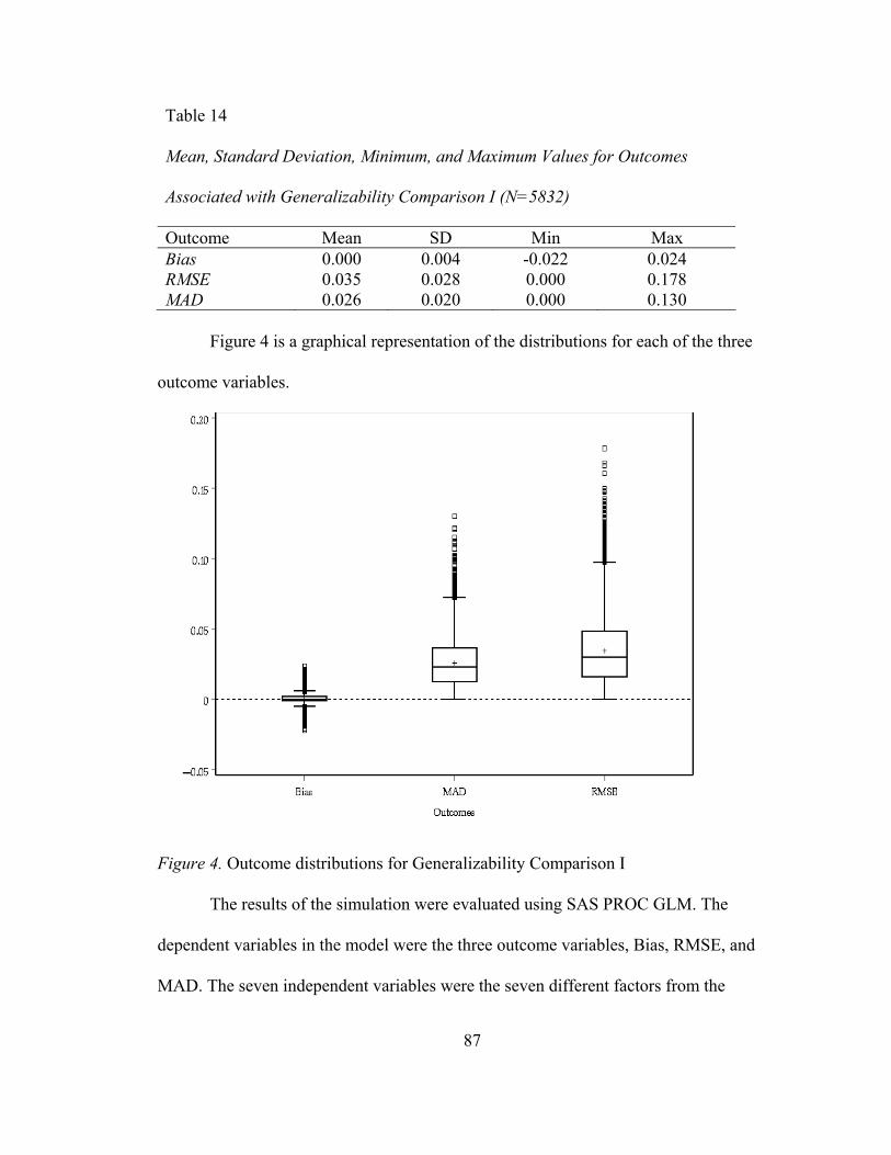
87
Table 14
Mean, Standard Deviation, Minimum, and Maximum Values for Outcomes
Associated with Generalizability Comparison I (N=5832)
Outcome Mean SD Min Max Bias 0.000 0.004 -0.022 0.024 RMSE 0.035 0.028 0.000 0.178 MAD 0.026 0.020 0.000 0.130
Figure 4 is a graphical representation of the distributions for each of the three
outcome variables.
Figure 4. Outcome distributions for Generalizability Comparison I
The results of the simulation were evaluated using SAS PROC GLM. The
dependent variables in the model were the three outcome variables, Bias, RMSE, and
MAD. The seven independent variables were the seven different factors from the
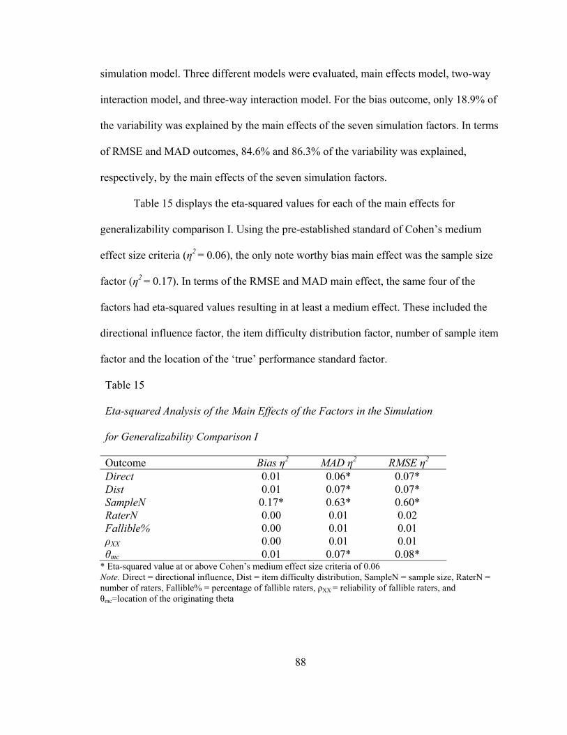
88
simulation model. Three different models were evaluated, main effects model, two-way
interaction model, and three-way interaction model. For the bias outcome, only 18.9% of
the variability was explained by the main effects of the seven simulation factors. In terms
of RMSE and MAD outcomes, 84.6% and 86.3% of the variability was explained,
respectively, by the main effects of the seven simulation factors.
Table 15 displays the eta-squared values for each of the main effects for
generalizability comparison I. Using the pre-established standard of Cohen’s medium
effect size criteria (η2 = 0.06), the only note worthy bias main effect was the sample size
factor (η2 = 0.17). In terms of the RMSE and MAD main effect, the same four of the
factors had eta-squared values resulting in at least a medium effect. These included the
directional influence factor, the item difficulty distribution factor, number of sample item
factor and the location of the ‘true’ performance standard factor.
Table 15
Eta-squared Analysis of the Main Effects of the Factors in the Simulation
for Generalizability Comparison I
Outcome Bias η2 MAD η2 RMSE η2 Direct 0.01 0.06* 0.07* Dist 0.01 0.07* 0.07* SampleN 0.17* 0.63* 0.60* RaterN 0.00 0.01 0.02 Fallible% 0.00 0.01 0.01 ρXX 0.00 0.01 0.01 θmc 0.01 0.07* 0.08*
* Eta-squared value at or above Cohen’s medium effect size criteria of 0.06 Note. Direct = directional influence, Dist = item difficulty distribution, SampleN = sample size, RaterN = number of raters, Fallible% = percentage of fallible raters, ρXX = reliability of fallible raters, and θmc=location of the originating theta
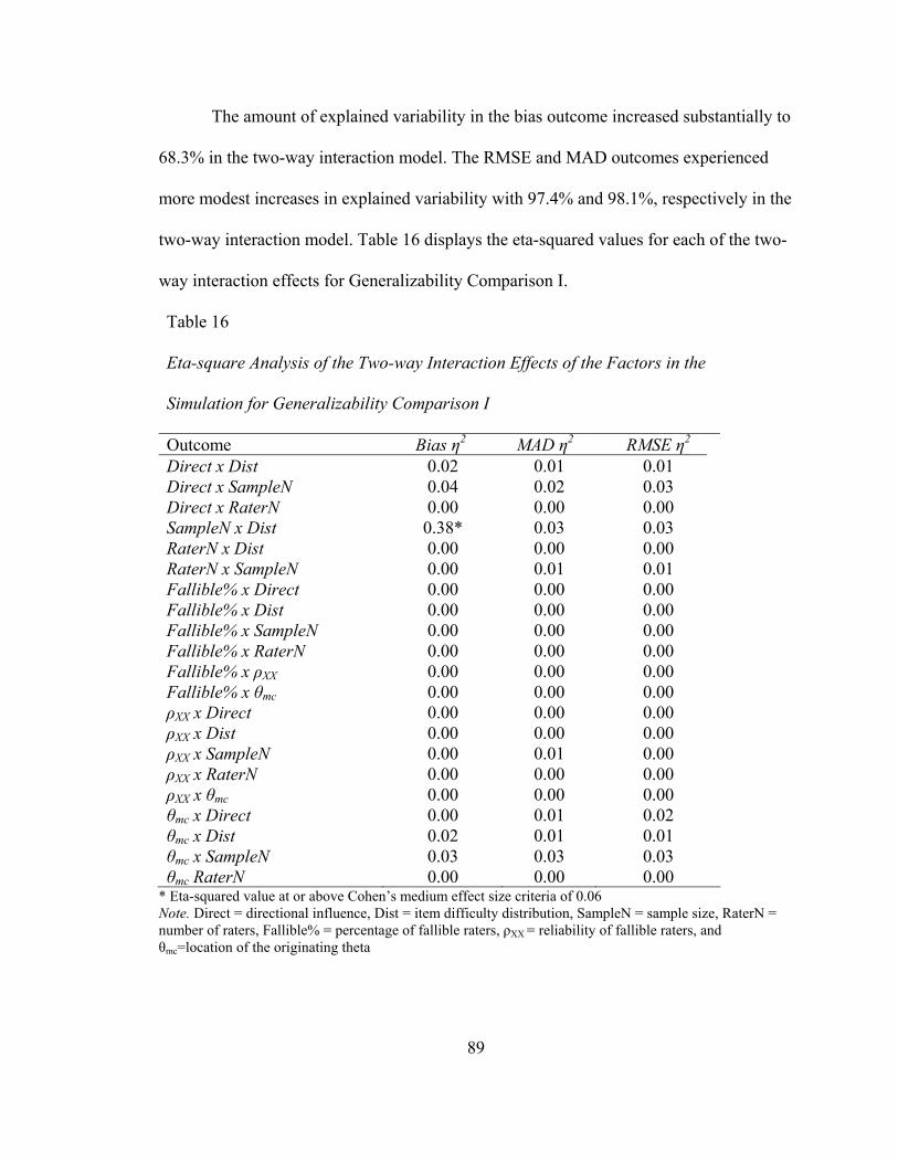
89
The amount of explained variability in the bias outcome increased substantially to
68.3% in the two-way interaction model. The RMSE and MAD outcomes experienced
more modest increases in explained variability with 97.4% and 98.1%, respectively in the
two-way interaction model. Table 16 displays the eta-squared values for each of the two-
way interaction effects for Generalizability Comparison I.
Table 16
Eta-square Analysis of the Two-way Interaction Effects of the Factors in the
Simulation for Generalizability Comparison I
Outcome Bias η2 MAD η2 RMSE η2 Direct x Dist 0.02 0.01 0.01 Direct x SampleN 0.04 0.02 0.03 Direct x RaterN 0.00 0.00 0.00 SampleN x Dist 0.38* 0.03 0.03 RaterN x Dist 0.00 0.00 0.00 RaterN x SampleN 0.00 0.01 0.01 Fallible% x Direct 0.00 0.00 0.00 Fallible% x Dist 0.00 0.00 0.00 Fallible% x SampleN 0.00 0.00 0.00 Fallible% x RaterN 0.00 0.00 0.00 Fallible% x ρXX 0.00 0.00 0.00 Fallible% x θmc 0.00 0.00 0.00 ρXX x Direct 0.00 0.00 0.00 ρXX x Dist 0.00 0.00 0.00 ρXX x SampleN 0.00 0.01 0.00 ρXX x RaterN 0.00 0.00 0.00 ρXX x θmc 0.00 0.00 0.00 θmc x Direct 0.00 0.01 0.02 θmc x Dist 0.02 0.01 0.01 θmc x SampleN 0.03 0.03 0.03 θmc RaterN 0.00 0.00 0.00
* Eta-squared value at or above Cohen’s medium effect size criteria of 0.06 Note. Direct = directional influence, Dist = item difficulty distribution, SampleN = sample size, RaterN = number of raters, Fallible% = percentage of fallible raters, ρXX = reliability of fallible raters, and θmc=location of the originating theta
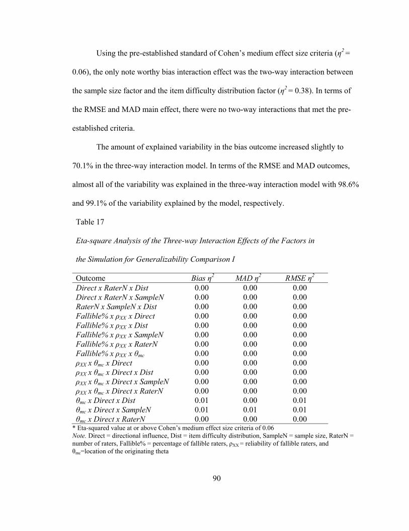
90
Using the pre-established standard of Cohen’s medium effect size criteria (η2 =
0.06), the only note worthy bias interaction effect was the two-way interaction between
the sample size factor and the item difficulty distribution factor (η2 = 0.38). In terms of
the RMSE and MAD main effect, there were no two-way interactions that met the pre-
established criteria.
The amount of explained variability in the bias outcome increased slightly to
70.1% in the three-way interaction model. In terms of the RMSE and MAD outcomes,
almost all of the variability was explained in the three-way interaction model with 98.6%
and 99.1% of the variability explained by the model, respectively.
Table 17
Eta-square Analysis of the Three-way Interaction Effects of the Factors in
the Simulation for Generalizability Comparison I
Outcome Bias η2 MAD η2 RMSE η2 Direct x RaterN x Dist 0.00 0.00 0.00 Direct x RaterN x SampleN 0.00 0.00 0.00 RaterN x SampleN x Dist 0.00 0.00 0.00 Fallible% x ρXX x Direct 0.00 0.00 0.00 Fallible% x ρXX x Dist 0.00 0.00 0.00 Fallible% x ρXX x SampleN 0.00 0.00 0.00 Fallible% x ρXX x RaterN 0.00 0.00 0.00 Fallible% x ρXX x θmc 0.00 0.00 0.00 ρXX x θmc x Direct 0.00 0.00 0.00 ρXX x θmc x Direct x Dist 0.00 0.00 0.00 ρXX x θmc x Direct x SampleN 0.00 0.00 0.00 ρXX x θmc x Direct x RaterN 0.00 0.00 0.00 θmc x Direct x Dist 0.01 0.00 0.01 θmc x Direct x SampleN 0.01 0.01 0.01 θmc x Direct x RaterN 0.00 0.00 0.00
* Eta-squared value at or above Cohen’s medium effect size criteria of 0.06 Note. Direct = directional influence, Dist = item difficulty distribution, SampleN = sample size, RaterN = number of raters, Fallible% = percentage of fallible raters, ρXX = reliability of fallible raters, and θmc=location of the originating theta
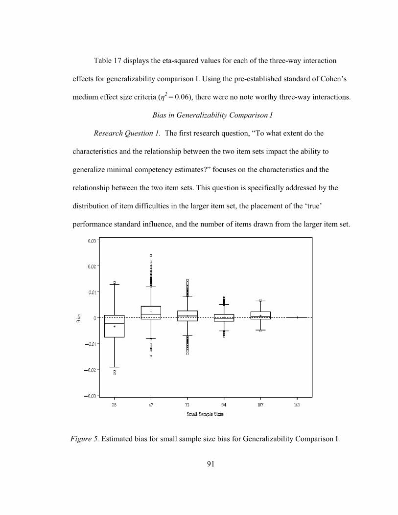
91
Table 17 displays the eta-squared values for each of the three-way interaction
effects for generalizability comparison I. Using the pre-established standard of Cohen’s
medium effect size criteria (η2 = 0.06), there were no note worthy three-way interactions.
Bias in Generalizability Comparison I
Research Question 1. The first research question, “To what extent do the
characteristics and the relationship between the two item sets impact the ability to
generalize minimal competency estimates?” focuses on the characteristics and the
relationship between the two item sets. This question is specifically addressed by the
distribution of item difficulties in the larger item set, the placement of the ‘true’
performance standard influence, and the number of items drawn from the larger item set.
Figure 5. Estimated bias for small sample size bias for Generalizability Comparison I.
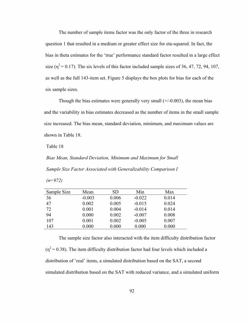
92
The number of sample items factor was the only factor of the three in research
question 1 that resulted in a medium or greater effect size for eta-squared. In fact, the
bias in theta estimates for the ‘true’ performance standard factor resulted in a large effect
size (η2 = 0.17). The six levels of this factor included sample sizes of 36, 47, 72, 94, 107,
as well as the full 143-item set. Figure 5 displays the box plots for bias for each of the
six sample sizes.
Though the bias estimates were generally very small (+/-0.003), the mean bias
and the variability in bias estimates decreased as the number of items in the small sample
size increased. The bias mean, standard deviation, minimum, and maximum values are
shown in Table 18.
Table 18
Bias Mean, Standard Deviation, Minimum and Maximum for Small
Sample Size Factor Associated with Generalizability Comparison I
(n=972)
Sample Size Mean SD Min Max 36 -0.003 0.006 -0.022 0.014 47 0.002 0.005 -0.015 0.024 72 0.001 0.004 -0.014 0.014 94 0.000 0.002 -0.007 0.008 107 0.001 0.002 -0.005 0.007 143 0.000 0.000 0.000 0.000
The sample size factor also interacted with the item difficulty distribution factor
(η2 = 0.38). The item difficulty distribution factor had four levels which included a
distribution of ‘real’ items, a simulated distribution based on the SAT, a second
simulated distribution based on the SAT with reduced variance, and a simulated uniform
93
distribution. The bias in theta estimates for the item difficulty distributions factor was
relatively small (η2 = 0.01). Figure 6 graphically displays this two-way interaction
between the sample size and item difficulty distribution factor. The results of the
simulation suggest that there was more variability in average bias estimates when the
sample size was small with the variability in average bias estimates decreasing as the
sample size increased. The average bias was the greatest in the simulated uniform
distribution, which initially was negatively bias in the 36-item small and was positively
bias for the remaining samples.
Figure 6. Two-way bias interaction between item difficulty distributions and small
sample size for Generalizability Comparison I.
94
The last factor in research question 1, placement of the ‘true’ performance
standard, had three levels which included an originating theta of -1, 0, and 1. The
variance in bias in theta estimates associated with the ‘true’ performance standard factor
was relatively small (η2 = 0.01).
Research Question 2. The second research question, “To what extent do the
characteristics of the standard setting process impact the ability to generalize minimal
competency estimates?” focuses on the characteristics of the standard setting process.
This question is specifically addressed by the number of raters, the percentage and
magnitude of ‘unreliable’ raters, and the impact of group dynamics and discussion
during the later rounds of the standard setting process.
None of the four factors in research question 2 resulted in a medium or larger
effect size in eta-squared. The number of raters factor had three levels which included 8,
12, and 16 raters involved in the standard setting process. The variance in estimated bias
in theta estimates associated with the number of raters factor was very small (η2 = 0.00).
The percentage of unreliable raters factor also had three levels which included 25%,
50%, and 75% of raters which were unreliable in their estimates. The effect size for the
estimated bias in theta estimates associated with the percentage of unreliable raters
factor was also small (η2 = 0.00). The magnitude of ‘unreliability’ factor had three levels
which included reliabilities (ρXX) of .65, .75, and .85. The variance in estimated bias in
theta estimates associated with the magnitude of ‘unreliability’ factor was also very
small (η2 = 0.00). The directional influence factor had three levels of this factor for the
directional impact of group dynamics and discussion. They included influence towards
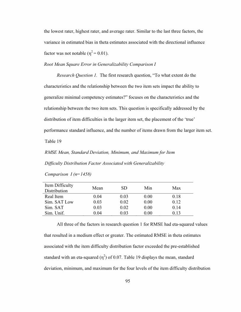
95
the lowest rater, highest rater, and average rater. Similar to the last three factors, the
variance in estimated bias in theta estimates associated with the directional influence
factor was not notable (η2 = 0.01).
Root Mean Square Error in Generalizability Comparison I
Research Question 1. The first research question, “To what extent do the
characteristics and the relationship between the two item sets impact the ability to
generalize minimal competency estimates?” focuses on the characteristics and the
relationship between the two item sets. This question is specifically addressed by the
distribution of item difficulties in the larger item set, the placement of the ‘true’
performance standard influence, and the number of items drawn from the larger item set.
Table 19
RMSE Mean, Standard Deviation, Minimum, and Maximum for Item
Difficulty Distribution Factor Associated with Generalizability
Comparison I (n=1458)
Item Difficulty Distribution Mean SD Min Max
Real Item 0.04 0.03 0.00 0.18 Sim. SAT Low 0.03 0.02 0.00 0.12 Sim. SAT 0.03 0.02 0.00 0.14 Sim. Unif. 0.04 0.03 0.00 0.13
All three of the factors in research question 1 for RMSE had eta-squared values
that resulted in a medium effect or greater. The estimated RMSE in theta estimates
associated with the item difficulty distribution factor exceeded the pre-established
standard with an eta-squared (η2) of 0.07. Table 19 displays the mean, standard
deviation, minimum, and maximum for the four levels of the item difficulty distribution
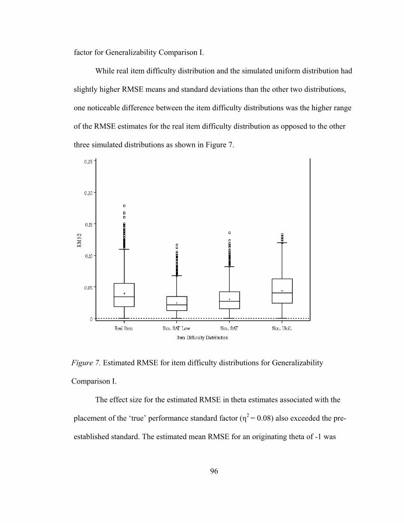
96
factor for Generalizability Comparison I.
While real item difficulty distribution and the simulated uniform distribution had
slightly higher RMSE means and standard deviations than the other two distributions,
one noticeable difference between the item difficulty distributions was the higher range
of the RMSE estimates for the real item difficulty distribution as opposed to the other
three simulated distributions as shown in Figure 7.
Figure 7. Estimated RMSE for item difficulty distributions for Generalizability
Comparison I.
The effect size for the estimated RMSE in theta estimates associated with the
placement of the ‘true’ performance standard factor (η2 = 0.08) also exceeded the pre-
established standard. The estimated mean RMSE for an originating theta of -1 was
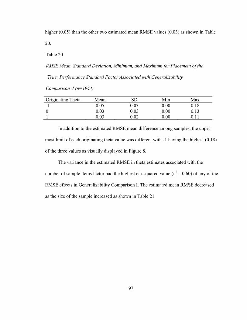
97
higher (0.05) than the other two estimated mean RMSE values (0.03) as shown in Table
20.
Table 20
RMSE Mean, Standard Deviation, Minimum, and Maximum for Placement of the
‘True’ Performance Standard Factor Associated with Generalizability
Comparison I (n=1944)
Originating Theta Mean SD Min Max -1 0.05 0.03 0.00 0.18 0 0.03 0.03 0.00 0.13 1 0.03 0.02 0.00 0.11
In addition to the estimated RMSE mean difference among samples, the upper
most limit of each originating theta value was different with -1 having the highest (0.18)
of the three values as visually displayed in Figure 8.
The variance in the estimated RMSE in theta estimates associated with the
number of sample items factor had the highest eta-squared value (η2 = 0.60) of any of the
RMSE effects in Generalizability Comparison I. The estimated mean RMSE decreased
as the size of the sample increased as shown in Table 21.
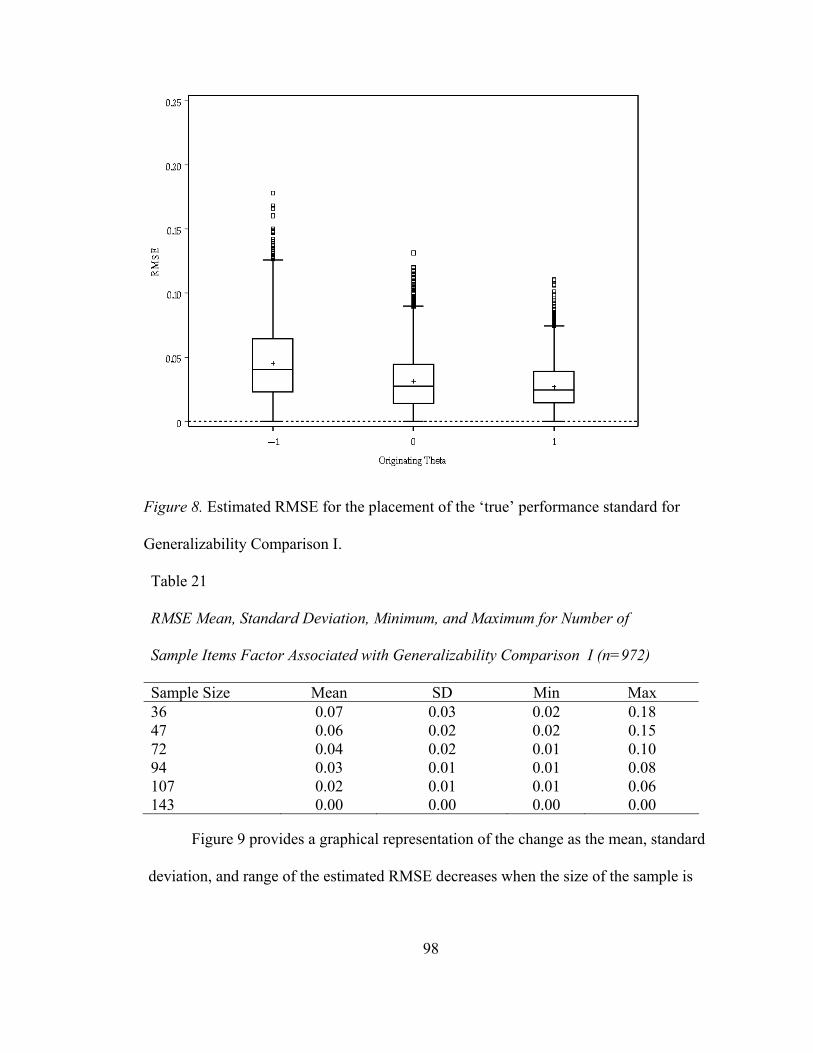
98
Figure 8. Estimated RMSE for the placement of the ‘true’ performance standard for
Generalizability Comparison I.
Table 21
RMSE Mean, Standard Deviation, Minimum, and Maximum for Number of
Sample Items Factor Associated with Generalizability Comparison I (n=972)
Sample Size Mean SD Min Max 36 0.07 0.03 0.02 0.18 47 0.06 0.02 0.02 0.15 72 0.04 0.02 0.01 0.10 94 0.03 0.01 0.01 0.08 107 0.02 0.01 0.01 0.06 143 0.00 0.00 0.00 0.00
Figure 9 provides a graphical representation of the change as the mean, standard
deviation, and range of the estimated RMSE decreases when the size of the sample is
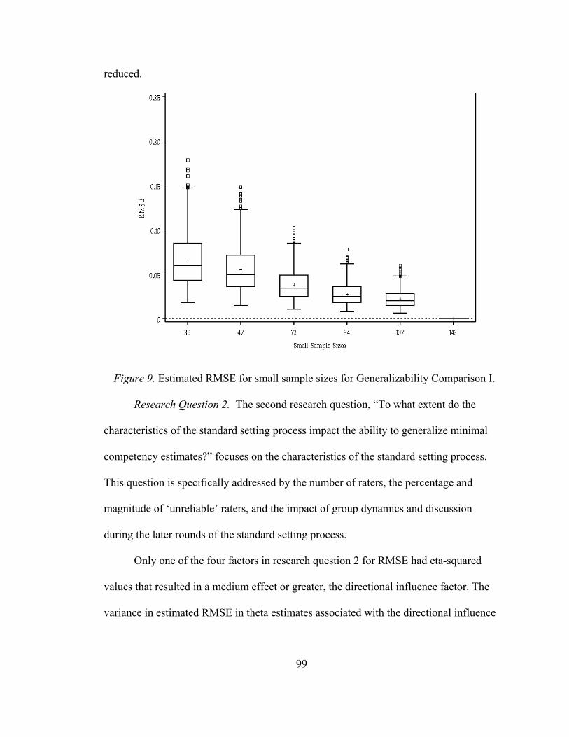
99
reduced.
Figure 9. Estimated RMSE for small sample sizes for Generalizability Comparison I.
Research Question 2. The second research question, “To what extent do the
characteristics of the standard setting process impact the ability to generalize minimal
competency estimates?” focuses on the characteristics of the standard setting process.
This question is specifically addressed by the number of raters, the percentage and
magnitude of ‘unreliable’ raters, and the impact of group dynamics and discussion
during the later rounds of the standard setting process.
Only one of the four factors in research question 2 for RMSE had eta-squared
values that resulted in a medium effect or greater, the directional influence factor. The
variance in estimated RMSE in theta estimates associated with the directional influence
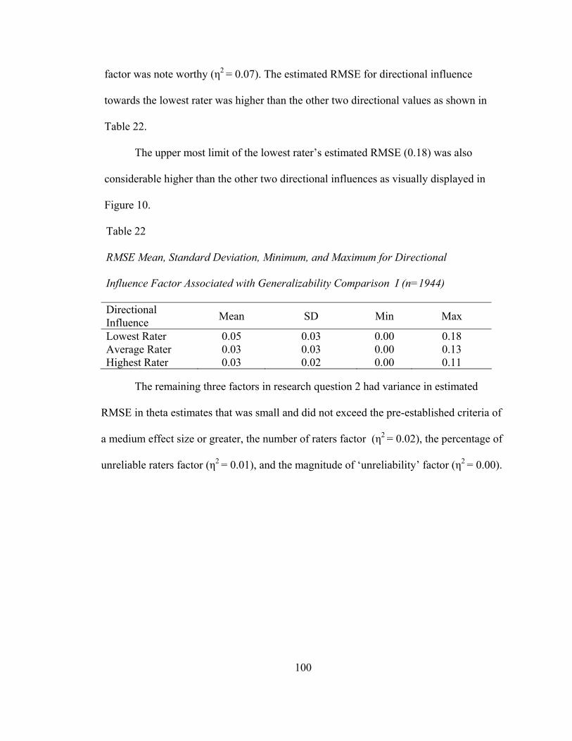
100
factor was note worthy (η2 = 0.07). The estimated RMSE for directional influence
towards the lowest rater was higher than the other two directional values as shown in
Table 22.
The upper most limit of the lowest rater’s estimated RMSE (0.18) was also
considerable higher than the other two directional influences as visually displayed in
Figure 10.
Table 22
RMSE Mean, Standard Deviation, Minimum, and Maximum for Directional
Influence Factor Associated with Generalizability Comparison I (n=1944)
Directional Influence Mean SD Min Max
Lowest Rater 0.05 0.03 0.00 0.18 Average Rater 0.03 0.03 0.00 0.13 Highest Rater 0.03 0.02 0.00 0.11
The remaining three factors in research question 2 had variance in estimated
RMSE in theta estimates that was small and did not exceed the pre-established criteria of
a medium effect size or greater, the number of raters factor (η2 = 0.02), the percentage of
unreliable raters factor (η2 = 0.01), and the magnitude of ‘unreliability’ factor (η2 = 0.00).
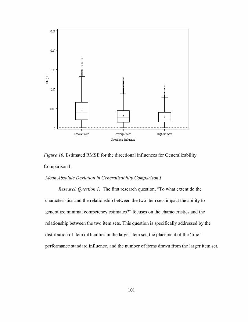
101
Figure 10. Estimated RMSE for the directional influences for Generalizability
Comparison I.
Mean Absolute Deviation in Generalizability Comparison I
Research Question 1. The first research question, “To what extent do the
characteristics and the relationship between the two item sets impact the ability to
generalize minimal competency estimates?” focuses on the characteristics and the
relationship between the two item sets. This question is specifically addressed by the
distribution of item difficulties in the larger item set, the placement of the ‘true’
performance standard influence, and the number of items drawn from the larger item set.
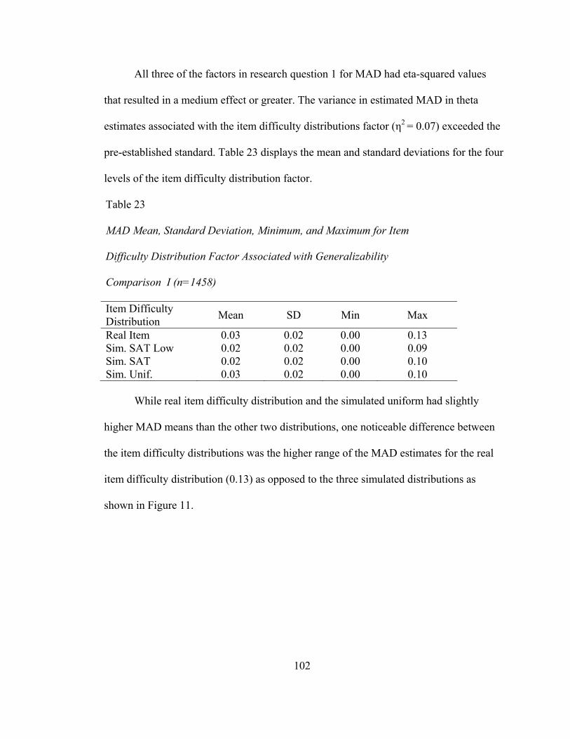
102
All three of the factors in research question 1 for MAD had eta-squared values
that resulted in a medium effect or greater. The variance in estimated MAD in theta
estimates associated with the item difficulty distributions factor (η2 = 0.07) exceeded the
pre-established standard. Table 23 displays the mean and standard deviations for the four
levels of the item difficulty distribution factor.
Table 23
MAD Mean, Standard Deviation, Minimum, and Maximum for Item
Difficulty Distribution Factor Associated with Generalizability
Comparison I (n=1458)
Item Difficulty Distribution Mean SD Min Max
Real Item 0.03 0.02 0.00 0.13 Sim. SAT Low 0.02 0.02 0.00 0.09 Sim. SAT 0.02 0.02 0.00 0.10 Sim. Unif. 0.03 0.02 0.00 0.10
While real item difficulty distribution and the simulated uniform had slightly
higher MAD means than the other two distributions, one noticeable difference between
the item difficulty distributions was the higher range of the MAD estimates for the real
item difficulty distribution (0.13) as opposed to the three simulated distributions as
shown in Figure 11.
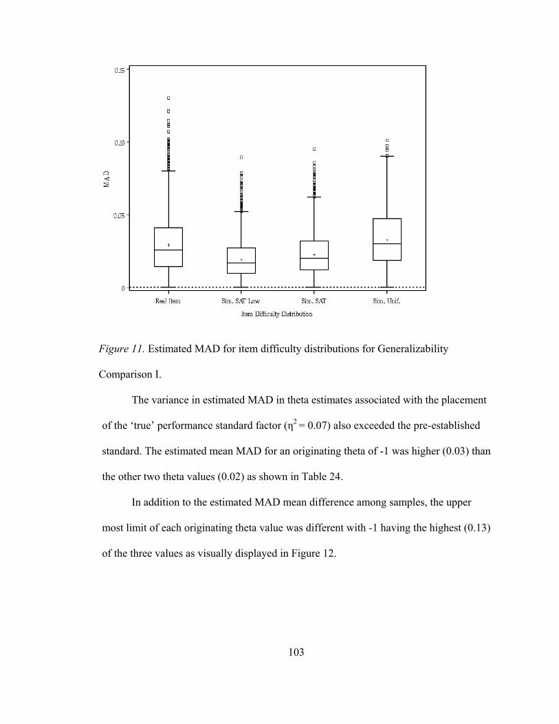
103
Figure 11. Estimated MAD for item difficulty distributions for Generalizability
Comparison I.
The variance in estimated MAD in theta estimates associated with the placement
of the ‘true’ performance standard factor (η2 = 0.07) also exceeded the pre-established
standard. The estimated mean MAD for an originating theta of -1 was higher (0.03) than
the other two theta values (0.02) as shown in Table 24.
In addition to the estimated MAD mean difference among samples, the upper
most limit of each originating theta value was different with -1 having the highest (0.13)
of the three values as visually displayed in Figure 12.
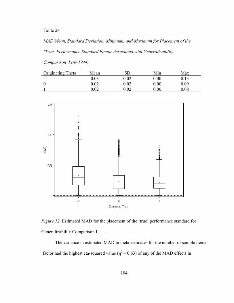
104
Table 24
MAD Mean, Standard Deviation, Minimum, and Maximum for Placement of the
‘True’ Performance Standard Factor Associated with Generalizability
Comparison I (n=1944)
Originating Theta Mean SD Min Max -1 0.03 0.02 0.00 0.13 0 0.02 0.02 0.00 0.09 1 0.02 0.02 0.00 0.08
Figure 12. Estimated MAD for the placement of the ‘true’ performance standard for
Generalizability Comparison I.
The variance in estimated MAD in theta estimates for the number of sample items
factor had the highest eta-squared value (η2 = 0.63) of any of the MAD effects in
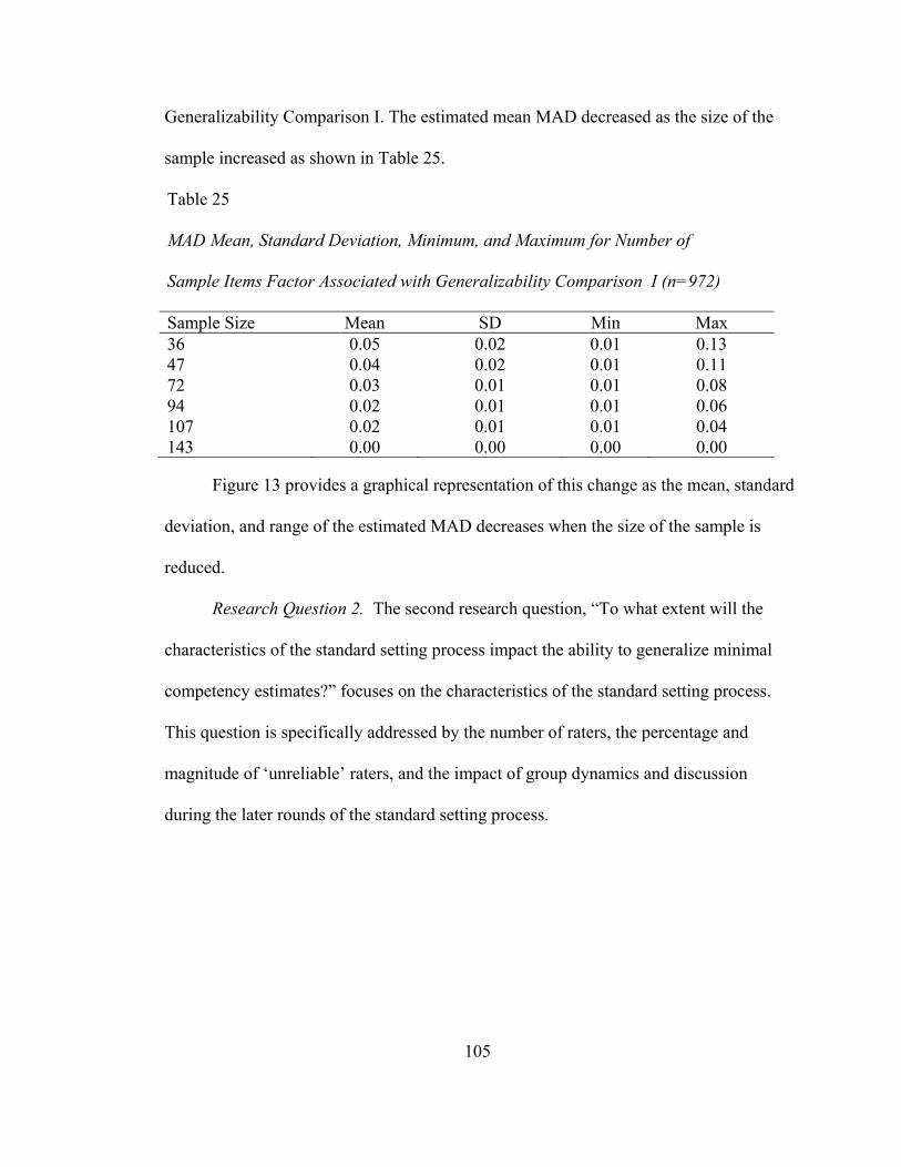
105
Generalizability Comparison I. The estimated mean MAD decreased as the size of the
sample increased as shown in Table 25.
Table 25
MAD Mean, Standard Deviation, Minimum, and Maximum for Number of
Sample Items Factor Associated with Generalizability Comparison I (n=972)
Sample Size Mean SD Min Max 36 0.05 0.02 0.01 0.13 47 0.04 0.02 0.01 0.11 72 0.03 0.01 0.01 0.08 94 0.02 0.01 0.01 0.06 107 0.02 0.01 0.01 0.04 143 0.00 0.00 0.00 0.00
Figure 13 provides a graphical representation of this change as the mean, standard
deviation, and range of the estimated MAD decreases when the size of the sample is
reduced.
Research Question 2. The second research question, “To what extent will the
characteristics of the standard setting process impact the ability to generalize minimal
competency estimates?” focuses on the characteristics of the standard setting process.
This question is specifically addressed by the number of raters, the percentage and
magnitude of ‘unreliable’ raters, and the impact of group dynamics and discussion
during the later rounds of the standard setting process.
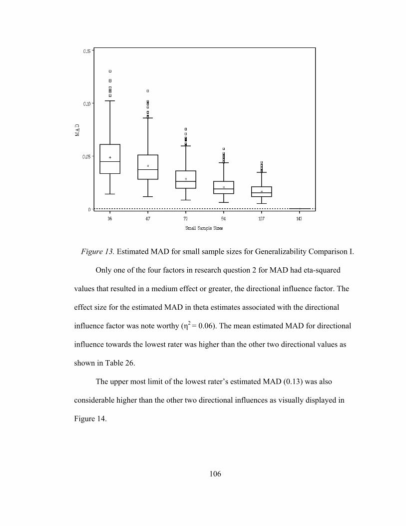
106
Figure 13. Estimated MAD for small sample sizes for Generalizability Comparison I.
Only one of the four factors in research question 2 for MAD had eta-squared
values that resulted in a medium effect or greater, the directional influence factor. The
effect size for the estimated MAD in theta estimates associated with the directional
influence factor was note worthy (η2 = 0.06). The mean estimated MAD for directional
influence towards the lowest rater was higher than the other two directional values as
shown in Table 26.
The upper most limit of the lowest rater’s estimated MAD (0.13) was also
considerable higher than the other two directional influences as visually displayed in
Figure 14.
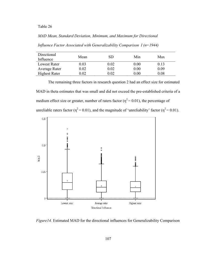
107
Table 26
MAD Mean, Standard Deviation, Minimum, and Maximum for Directional
Influence Factor Associated with Generalizability Comparison I (n=1944)
Directional Influence Mean SD Min Max
Lowest Rater 0.03 0.02 0.00 0.13 Average Rater 0.02 0.02 0.00 0.09 Highest Rater 0.02 0.02 0.00 0.08
The remaining three factors in research question 2 had an effect size for estimated
MAD in theta estimates that was small and did not exceed the pre-established criteria of a
medium effect size or greater, number of raters factor (η2 = 0.01), the percentage of
unreliable raters factor (η2 = 0.01), and the magnitude of ‘unreliability’ factor (η2 = 0.01).
Figure14. Estimated MAD for the directional influences for Generalizability Comparison
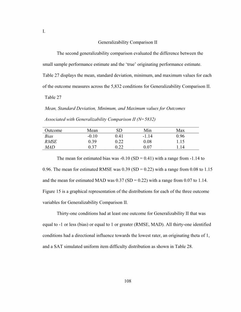
108
I.
Generalizability Comparison II
The second generalizability comparison evaluated the difference between the
small sample performance estimate and the ‘true’ originating performance estimate.
Table 27 displays the mean, standard deviation, minimum, and maximum values for each
of the outcome measures across the 5,832 conditions for Generalizability Comparison II.
Table 27
Mean, Standard Deviation, Minimum, and Maximum values for Outcomes
Associated with Generalizability Comparison II (N=5832)
Outcome Mean SD Min Max Bias -0.10 0.41 -1.14 0.96 RMSE 0.39 0.22 0.08 1.15 MAD 0.37 0.22 0.07 1.14
The mean for estimated bias was -0.10 (SD = 0.41) with a range from -1.14 to
0.96. The mean for estimated RMSE was 0.39 (SD = 0.22) with a range from 0.08 to 1.15
and the mean for estimated MAD was 0.37 (SD = 0.22) with a range from 0.07 to 1.14.
Figure 15 is a graphical representation of the distributions for each of the three outcome
variables for Generalizability Comparison II.
Thirty-one conditions had at least one outcome for Generalizability II that was
equal to -1 or less (bias) or equal to 1 or greater (RMSE, MAD). All thirty-one identified
conditions had a directional influence towards the lowest rater, an originating theta of 1,
and a SAT simulated uniform item difficulty distribution as shown in Table 28.
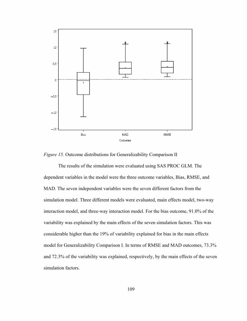
109
Figure 15. Outcome distributions for Generalizability Comparison II
The results of the simulation were evaluated using SAS PROC GLM. The
dependent variables in the model were the three outcome variables, Bias, RMSE, and
MAD. The seven independent variables were the seven different factors from the
simulation model. Three different models were evaluated, main effects model, two-way
interaction model, and three-way interaction model. For the bias outcome, 91.0% of the
variability was explained by the main effects of the seven simulation factors. This was
considerable higher than the 19% of variability explained for bias in the main effects
model for Generalizability Comparison I. In terms of RMSE and MAD outcomes, 73.3%
and 72.3% of the variability was explained, respectively, by the main effects of the seven
simulation factors.
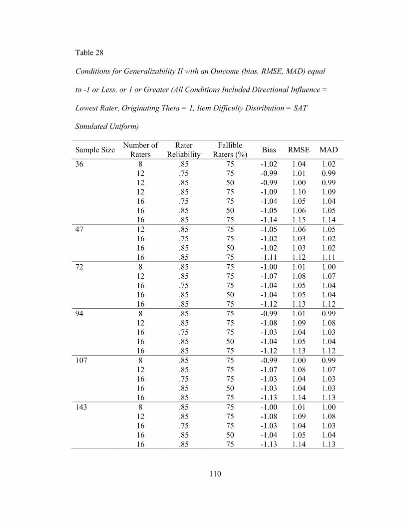
110
Table 28
Conditions for Generalizability II with an Outcome (bias, RMSE, MAD) equal
to -1 or Less, or 1 or Greater (All Conditions Included Directional Influence =
Lowest Rater, Originating Theta = 1, Item Difficulty Distribution = SAT
Simulated Uniform)
Sample Size Number of Raters
Rater Reliability
Fallible Raters (%) Bias RMSE MAD
36 8 .85 75 -1.02 1.04 1.02 12 .75 75 -0.99 1.01 0.99 12 .85 50 -0.99 1.00 0.99 12 .85 75 -1.09 1.10 1.09 16 .75 75 -1.04 1.05 1.04 16 .85 50 -1.05 1.06 1.05 16 .85 75 -1.14 1.15 1.14 47 12 .85 75 -1.05 1.06 1.05 16 .75 75 -1.02 1.03 1.02 16 .85 50 -1.02 1.03 1.02 16 .85 75 -1.11 1.12 1.11 72 8 .85 75 -1.00 1.01 1.00 12 .85 75 -1.07 1.08 1.07 16 .75 75 -1.04 1.05 1.04 16 .85 50 -1.04 1.05 1.04 16 .85 75 -1.12 1.13 1.12 94 8 .85 75 -0.99 1.01 0.99 12 .85 75 -1.08 1.09 1.08 16 .75 75 -1.03 1.04 1.03 16 .85 50 -1.04 1.05 1.04 16 .85 75 -1.12 1.13 1.12 107 8 .85 75 -0.99 1.00 0.99 12 .85 75 -1.07 1.08 1.07 16 .75 75 -1.03 1.04 1.03 16 .85 50 -1.03 1.04 1.03 16 .85 75 -1.13 1.14 1.13 143 8 .85 75 -1.00 1.01 1.00 12 .85 75 -1.08 1.09 1.08 16 .75 75 -1.03 1.04 1.03 16 .85 50 -1.04 1.05 1.04 16 .85 75 -1.13 1.14 1.13
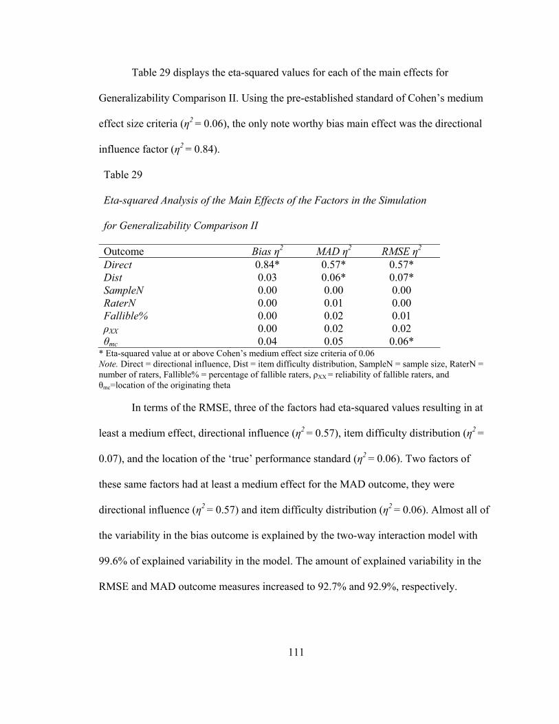
111
Table 29 displays the eta-squared values for each of the main effects for
Generalizability Comparison II. Using the pre-established standard of Cohen’s medium
effect size criteria (η2 = 0.06), the only note worthy bias main effect was the directional
influence factor (η2 = 0.84).
Table 29
Eta-squared Analysis of the Main Effects of the Factors in the Simulation
for Generalizability Comparison II
Outcome Bias η2 MAD η2 RMSE η2 Direct 0.84* 0.57* 0.57* Dist 0.03 0.06* 0.07* SampleN 0.00 0.00 0.00 RaterN 0.00 0.01 0.00 Fallible% 0.00 0.02 0.01 ρXX 0.00 0.02 0.02 θmc 0.04 0.05 0.06*
* Eta-squared value at or above Cohen’s medium effect size criteria of 0.06 Note. Direct = directional influence, Dist = item difficulty distribution, SampleN = sample size, RaterN = number of raters, Fallible% = percentage of fallible raters, ρXX = reliability of fallible raters, and θmc=location of the originating theta In terms of the RMSE, three of the factors had eta-squared values resulting in at
least a medium effect, directional influence (η2 = 0.57), item difficulty distribution (η2 =
0.07), and the location of the ‘true’ performance standard (η2 = 0.06). Two factors of
these same factors had at least a medium effect for the MAD outcome, they were
directional influence (η2 = 0.57) and item difficulty distribution (η2 = 0.06). Almost all of
the variability in the bias outcome is explained by the two-way interaction model with
99.6% of explained variability in the model. The amount of explained variability in the
RMSE and MAD outcome measures increased to 92.7% and 92.9%, respectively.
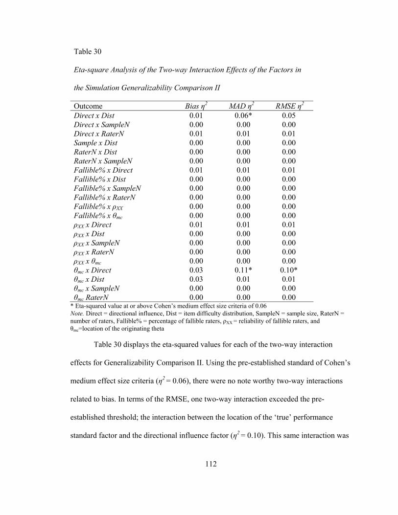
112
Table 30
Eta-square Analysis of the Two-way Interaction Effects of the Factors in
the Simulation Generalizability Comparison II
Outcome Bias η2 MAD η2 RMSE η2 Direct x Dist 0.01 0.06* 0.05 Direct x SampleN 0.00 0.00 0.00 Direct x RaterN 0.01 0.01 0.01 Sample x Dist 0.00 0.00 0.00 RaterN x Dist 0.00 0.00 0.00 RaterN x SampleN 0.00 0.00 0.00 Fallible% x Direct 0.01 0.01 0.01 Fallible% x Dist 0.00 0.00 0.00 Fallible% x SampleN 0.00 0.00 0.00 Fallible% x RaterN 0.00 0.00 0.00 Fallible% x ρXX 0.00 0.00 0.00 Fallible% x θmc 0.00 0.00 0.00 ρXX x Direct 0.01 0.01 0.01 ρXX x Dist 0.00 0.00 0.00 ρXX x SampleN 0.00 0.00 0.00 ρXX x RaterN 0.00 0.00 0.00 ρXX x θmc 0.00 0.00 0.00 θmc x Direct 0.03 0.11* 0.10* θmc x Dist 0.03 0.01 0.01 θmc x SampleN 0.00 0.00 0.00 θmc RaterN 0.00 0.00 0.00
* Eta-squared value at or above Cohen’s medium effect size criteria of 0.06 Note. Direct = directional influence, Dist = item difficulty distribution, SampleN = sample size, RaterN = number of raters, Fallible% = percentage of fallible raters, ρXX = reliability of fallible raters, and θmc=location of the originating theta Table 30 displays the eta-squared values for each of the two-way interaction
effects for Generalizability Comparison II. Using the pre-established standard of Cohen’s
medium effect size criteria (η2 = 0.06), there were no note worthy two-way interactions
related to bias. In terms of the RMSE, one two-way interaction exceeded the pre-
established threshold; the interaction between the location of the ‘true’ performance
standard factor and the directional influence factor (η2 = 0.10). This same interaction was
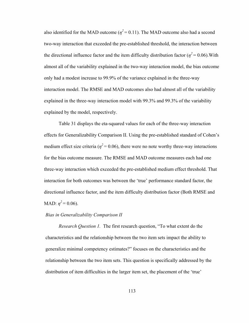
113
also identified for the MAD outcome (η2 = 0.11). The MAD outcome also had a second
two-way interaction that exceeded the pre-established threshold, the interaction between
the directional influence factor and the item difficulty distribution factor (η2 = 0.06).With
almost all of the variability explained in the two-way interaction model, the bias outcome
only had a modest increase to 99.9% of the variance explained in the three-way
interaction model. The RMSE and MAD outcomes also had almost all of the variability
explained in the three-way interaction model with 99.3% and 99.3% of the variability
explained by the model, respectively.
Table 31 displays the eta-squared values for each of the three-way interaction
effects for Generalizability Comparison II. Using the pre-established standard of Cohen’s
medium effect size criteria (η2 = 0.06), there were no note worthy three-way interactions
for the bias outcome measure. The RMSE and MAD outcome measures each had one
three-way interaction which exceeded the pre-established medium effect threshold. That
interaction for both outcomes was between the ‘true’ performance standard factor, the
directional influence factor, and the item difficulty distribution factor (Both RMSE and
MAD: η2 = 0.06).
Bias in Generalizability Comparison II
Research Question 1. The first research question, “To what extent do the
characteristics and the relationship between the two item sets impact the ability to
generalize minimal competency estimates?” focuses on the characteristics and the
relationship between the two item sets. This question is specifically addressed by the
distribution of item difficulties in the larger item set, the placement of the ‘true’
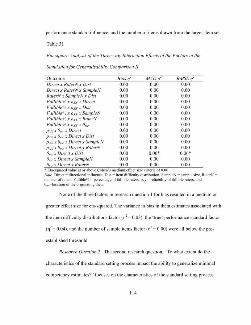
114
performance standard influence, and the number of items drawn from the larger item set.
Table 31
Eta-square Analysis of the Three-way Interaction Effects of the Factors in the
Simulation for Generalizability Comparison II
Outcome Bias η2 MAD η2 RMSE η2 Direct x RaterN x Dist 0.00 0.00 0.00 Direct x RaterN x SampleN 0.00 0.00 0.00 RaterN x SampleN x Dist 0.00 0.00 0.00 Fallible% x ρXX x Direct 0.00 0.00 0.00 Fallible% x ρXX x Dist 0.00 0.00 0.00 Fallible% x ρXX x SampleN 0.00 0.00 0.00 Fallible% x ρXX x RaterN 0.00 0.00 0.00 Fallible% x ρXX x θmc 0.00 0.00 0.00 ρXX x θmc x Direct 0.00 0.00 0.00 ρXX x θmc x Direct x Dist 0.00 0.00 0.00 ρXX x θmc x Direct x SampleN 0.00 0.00 0.00 ρXX x θmc x Direct x RaterN 0.00 0.00 0.00 θmc x Direct x Dist 0.00 0.06* 0.06* θmc x Direct x SampleN 0.00 0.00 0.00 θmc x Direct x RaterN 0.00 0.00 0.00
* Eta-squared value at or above Cohen’s medium effect size criteria of 0.06 Note. Direct = directional influence, Dist = item difficulty distribution, SampleN = sample size, RaterN = number of raters, Fallible% = percentage of fallible raters, ρXX = reliability of fallible raters, and θmc=location of the originating theta
None of the three factors in research question 1 for bias resulted in a medium or
greater effect size for eta-squared. The variance in bias in theta estimates associated with
the item difficulty distributions factor (η2 = 0.03), the ‘true’ performance standard factor
(η2 = 0.04), and the number of sample items factor (η2 = 0.00) were all below the pre-
established threshold.
Research Question 2. The second research question, “To what extent do the
characteristics of the standard setting process impact the ability to generalize minimal
competency estimates?” focuses on the characteristics of the standard setting process.
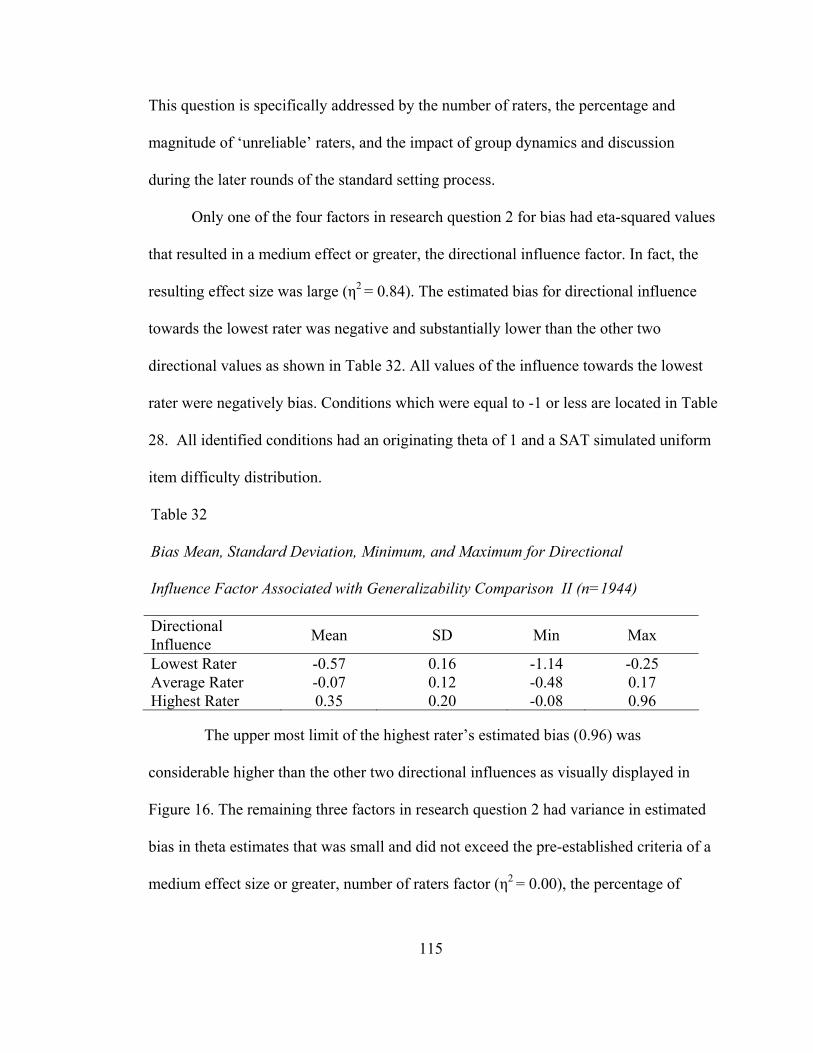
115
This question is specifically addressed by the number of raters, the percentage and
magnitude of ‘unreliable’ raters, and the impact of group dynamics and discussion
during the later rounds of the standard setting process.
Only one of the four factors in research question 2 for bias had eta-squared values
that resulted in a medium effect or greater, the directional influence factor. In fact, the
resulting effect size was large (η2 = 0.84). The estimated bias for directional influence
towards the lowest rater was negative and substantially lower than the other two
directional values as shown in Table 32. All values of the influence towards the lowest
rater were negatively bias. Conditions which were equal to -1 or less are located in Table
28. All identified conditions had an originating theta of 1 and a SAT simulated uniform
item difficulty distribution.
Table 32
Bias Mean, Standard Deviation, Minimum, and Maximum for Directional
Influence Factor Associated with Generalizability Comparison II (n=1944)
Directional Influence Mean SD Min Max
Lowest Rater -0.57 0.16 -1.14 -0.25 Average Rater -0.07 0.12 -0.48 0.17 Highest Rater 0.35 0.20 -0.08 0.96
The upper most limit of the highest rater’s estimated bias (0.96) was
considerable higher than the other two directional influences as visually displayed in
Figure 16. The remaining three factors in research question 2 had variance in estimated
bias in theta estimates that was small and did not exceed the pre-established criteria of a
medium effect size or greater, number of raters factor (η2 = 0.00), the percentage of
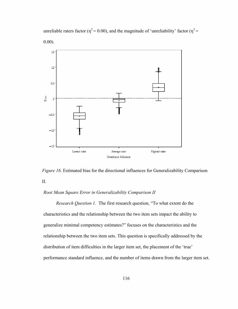
116
unreliable raters factor (η2 = 0.00), and the magnitude of ‘unreliability’ factor (η2 =
0.00).
Figure 16. Estimated bias for the directional influences for Generalizability Comparison
II.
Root Mean Square Error in Generalizability Comparison II
Research Question 1. The first research question, “To what extent do the
characteristics and the relationship between the two item sets impact the ability to
generalize minimal competency estimates?” focuses on the characteristics and the
relationship between the two item sets. This question is specifically addressed by the
distribution of item difficulties in the larger item set, the placement of the ‘true’
performance standard influence, and the number of items drawn from the larger item set.
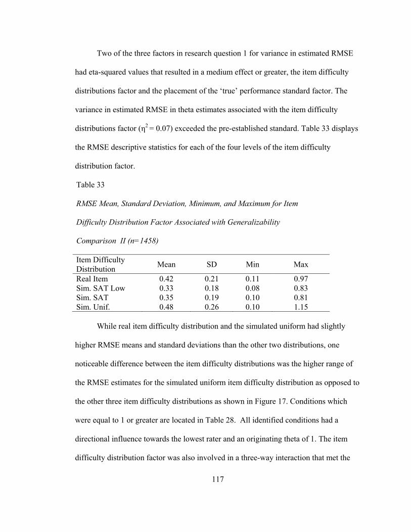
117
Two of the three factors in research question 1 for variance in estimated RMSE
had eta-squared values that resulted in a medium effect or greater, the item difficulty
distributions factor and the placement of the ‘true’ performance standard factor. The
variance in estimated RMSE in theta estimates associated with the item difficulty
distributions factor (η2 = 0.07) exceeded the pre-established standard. Table 33 displays
the RMSE descriptive statistics for each of the four levels of the item difficulty
distribution factor.
Table 33
RMSE Mean, Standard Deviation, Minimum, and Maximum for Item
Difficulty Distribution Factor Associated with Generalizability
Comparison II (n=1458)
Item Difficulty Distribution Mean SD Min Max
Real Item 0.42 0.21 0.11 0.97 Sim. SAT Low 0.33 0.18 0.08 0.83 Sim. SAT 0.35 0.19 0.10 0.81 Sim. Unif. 0.48 0.26 0.10 1.15
While real item difficulty distribution and the simulated uniform had slightly
higher RMSE means and standard deviations than the other two distributions, one
noticeable difference between the item difficulty distributions was the higher range of
the RMSE estimates for the simulated uniform item difficulty distribution as opposed to
the other three item difficulty distributions as shown in Figure 17. Conditions which
were equal to 1 or greater are located in Table 28. All identified conditions had a
directional influence towards the lowest rater and an originating theta of 1. The item
difficulty distribution factor was also involved in a three-way interaction that met the
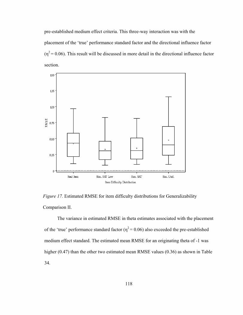
118
pre-established medium effect criteria. This three-way interaction was with the
placement of the ‘true’ performance standard factor and the directional influence factor
(η2 = 0.06). This result will be discussed in more detail in the directional influence factor
section.
Figure 17. Estimated RMSE for item difficulty distributions for Generalizability
Comparison II.
The variance in estimated RMSE in theta estimates associated with the placement
of the ‘true’ performance standard factor (η2 = 0.06) also exceeded the pre-established
medium effect standard. The estimated mean RMSE for an originating theta of -1 was
higher (0.47) than the other two estimated mean RMSE values (0.36) as shown in Table
34.
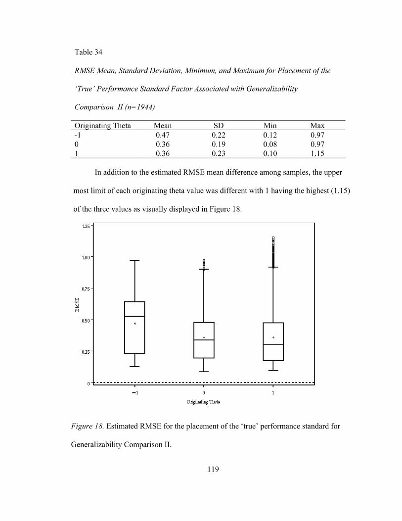
119
Table 34
RMSE Mean, Standard Deviation, Minimum, and Maximum for Placement of the
‘True’ Performance Standard Factor Associated with Generalizability
Comparison II (n=1944)
Originating Theta Mean SD Min Max -1 0.47 0.22 0.12 0.97 0 0.36 0.19 0.08 0.97 1 0.36 0.23 0.10 1.15
In addition to the estimated RMSE mean difference among samples, the upper
most limit of each originating theta value was different with 1 having the highest (1.15)
of the three values as visually displayed in Figure 18.
Figure 18. Estimated RMSE for the placement of the ‘true’ performance standard for
Generalizability Comparison II.
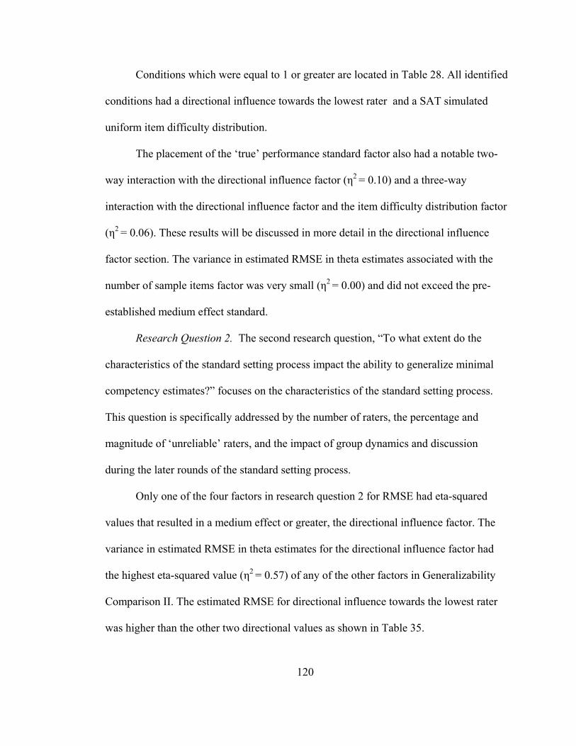
120
Conditions which were equal to 1 or greater are located in Table 28. All identified
conditions had a directional influence towards the lowest rater and a SAT simulated
uniform item difficulty distribution.
The placement of the ‘true’ performance standard factor also had a notable two-
way interaction with the directional influence factor (η2 = 0.10) and a three-way
interaction with the directional influence factor and the item difficulty distribution factor
(η2 = 0.06). These results will be discussed in more detail in the directional influence
factor section. The variance in estimated RMSE in theta estimates associated with the
number of sample items factor was very small (η2 = 0.00) and did not exceed the pre-
established medium effect standard.
Research Question 2. The second research question, “To what extent do the
characteristics of the standard setting process impact the ability to generalize minimal
competency estimates?” focuses on the characteristics of the standard setting process.
This question is specifically addressed by the number of raters, the percentage and
magnitude of ‘unreliable’ raters, and the impact of group dynamics and discussion
during the later rounds of the standard setting process.
Only one of the four factors in research question 2 for RMSE had eta-squared
values that resulted in a medium effect or greater, the directional influence factor. The
variance in estimated RMSE in theta estimates for the directional influence factor had
the highest eta-squared value (η2 = 0.57) of any of the other factors in Generalizability
Comparison II. The estimated RMSE for directional influence towards the lowest rater
was higher than the other two directional values as shown in Table 35.
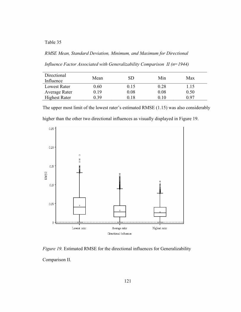
121
Table 35
RMSE Mean, Standard Deviation, Minimum, and Maximum for Directional
Influence Factor Associated with Generalizability Comparison II (n=1944)
Directional Influence Mean SD Min Max
Lowest Rater 0.60 0.15 0.28 1.15 Average Rater 0.19 0.08 0.08 0.50 Highest Rater 0.39 0.18 0.10 0.97
The upper most limit of the lowest rater’s estimated RMSE (1.15) was also considerably
higher than the other two directional influences as visually displayed in Figure 19.
Figure 19. Estimated RMSE for the directional influences for Generalizability
Comparison II.
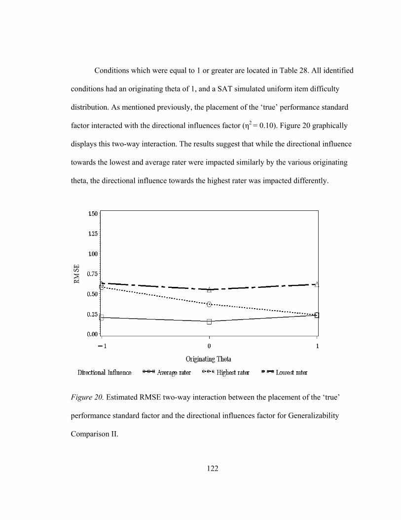
122
Conditions which were equal to 1 or greater are located in Table 28. All identified
conditions had an originating theta of 1, and a SAT simulated uniform item difficulty
distribution. As mentioned previously, the placement of the ‘true’ performance standard
factor interacted with the directional influences factor (η2 = 0.10). Figure 20 graphically
displays this two-way interaction. The results suggest that while the directional influence
towards the lowest and average rater were impacted similarly by the various originating
theta, the directional influence towards the highest rater was impacted differently.
Figure 20. Estimated RMSE two-way interaction between the placement of the ‘true’
performance standard factor and the directional influences factor for Generalizability
Comparison II.
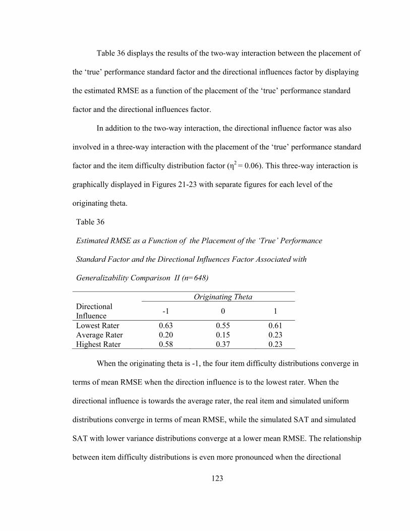
123
Table 36 displays the results of the two-way interaction between the placement of
the ‘true’ performance standard factor and the directional influences factor by displaying
the estimated RMSE as a function of the placement of the ‘true’ performance standard
factor and the directional influences factor.
In addition to the two-way interaction, the directional influence factor was also
involved in a three-way interaction with the placement of the ‘true’ performance standard
factor and the item difficulty distribution factor (η2 = 0.06). This three-way interaction is
graphically displayed in Figures 21-23 with separate figures for each level of the
originating theta.
Table 36
Estimated RMSE as a Function of the Placement of the ‘True’ Performance
Standard Factor and the Directional Influences Factor Associated with
Generalizability Comparison II (n=648)
Originating Theta Directional Influence -1 0 1
Lowest Rater 0.63 0.55 0.61 Average Rater 0.20 0.15 0.23 Highest Rater 0.58 0.37 0.23
When the originating theta is -1, the four item difficulty distributions converge in
terms of mean RMSE when the direction influence is to the lowest rater. When the
directional influence is towards the average rater, the real item and simulated uniform
distributions converge in terms of mean RMSE, while the simulated SAT and simulated
SAT with lower variance distributions converge at a lower mean RMSE. The relationship
between item difficulty distributions is even more pronounced when the directional
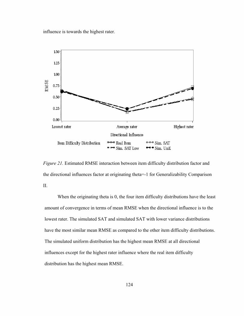
124
influence is towards the highest rater.
Figure 21. Estimated RMSE interaction between item difficulty distribution factor and
the directional influences factor at originating theta=-1 for Generalizability Comparison
II.
When the originating theta is 0, the four item difficulty distributions have the least
amount of convergence in terms of mean RMSE when the directional influence is to the
lowest rater. The simulated SAT and simulated SAT with lower variance distributions
have the most similar mean RMSE as compared to the other item difficulty distributions.
The simulated uniform distribution has the highest mean RMSE at all directional
influences except for the highest rater influence where the real item difficulty
distribution has the highest mean RMSE.
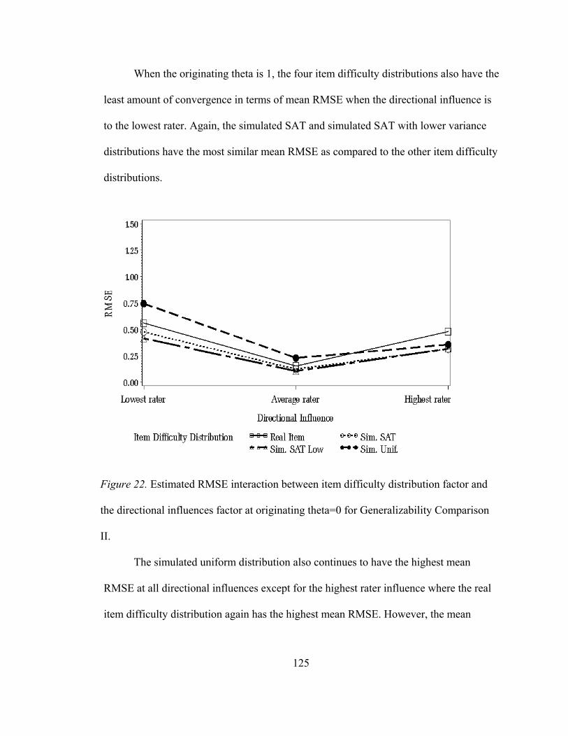
125
When the originating theta is 1, the four item difficulty distributions also have the
least amount of convergence in terms of mean RMSE when the directional influence is
to the lowest rater. Again, the simulated SAT and simulated SAT with lower variance
distributions have the most similar mean RMSE as compared to the other item difficulty
distributions.
Figure 22. Estimated RMSE interaction between item difficulty distribution factor and
the directional influences factor at originating theta=0 for Generalizability Comparison
II.
The simulated uniform distribution also continues to have the highest mean
RMSE at all directional influences except for the highest rater influence where the real
item difficulty distribution again has the highest mean RMSE. However, the mean
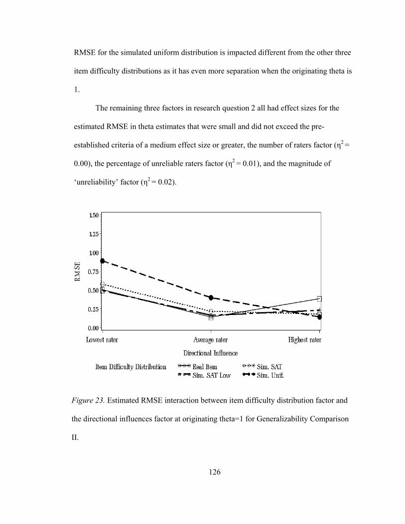
126
RMSE for the simulated uniform distribution is impacted different from the other three
item difficulty distributions as it has even more separation when the originating theta is
1.
The remaining three factors in research question 2 all had effect sizes for the
estimated RMSE in theta estimates that were small and did not exceed the pre-
established criteria of a medium effect size or greater, the number of raters factor (η2 =
0.00), the percentage of unreliable raters factor (η2 = 0.01), and the magnitude of
‘unreliability’ factor (η2 = 0.02).
Figure 23. Estimated RMSE interaction between item difficulty distribution factor and
the directional influences factor at originating theta=1 for Generalizability Comparison
II.
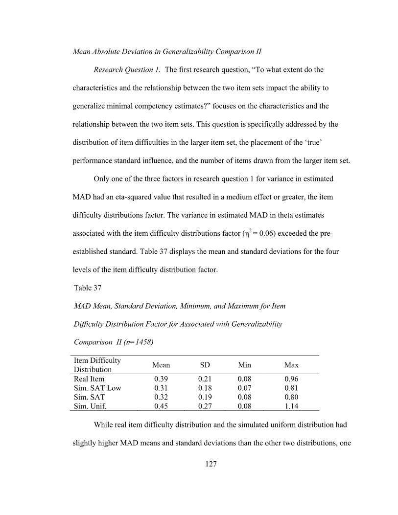
127
Mean Absolute Deviation in Generalizability Comparison II
Research Question 1. The first research question, “To what extent do the
characteristics and the relationship between the two item sets impact the ability to
generalize minimal competency estimates?” focuses on the characteristics and the
relationship between the two item sets. This question is specifically addressed by the
distribution of item difficulties in the larger item set, the placement of the ‘true’
performance standard influence, and the number of items drawn from the larger item set.
Only one of the three factors in research question 1 for variance in estimated
MAD had an eta-squared value that resulted in a medium effect or greater, the item
difficulty distributions factor. The variance in estimated MAD in theta estimates
associated with the item difficulty distributions factor (η2 = 0.06) exceeded the pre-
established standard. Table 37 displays the mean and standard deviations for the four
levels of the item difficulty distribution factor.
Table 37
MAD Mean, Standard Deviation, Minimum, and Maximum for Item
Difficulty Distribution Factor for Associated with Generalizability
Comparison II (n=1458)
Item Difficulty Distribution Mean SD Min Max
Real Item 0.39 0.21 0.08 0.96 Sim. SAT Low 0.31 0.18 0.07 0.81 Sim. SAT 0.32 0.19 0.08 0.80 Sim. Unif. 0.45 0.27 0.08 1.14
While real item difficulty distribution and the simulated uniform distribution had
slightly higher MAD means and standard deviations than the other two distributions, one
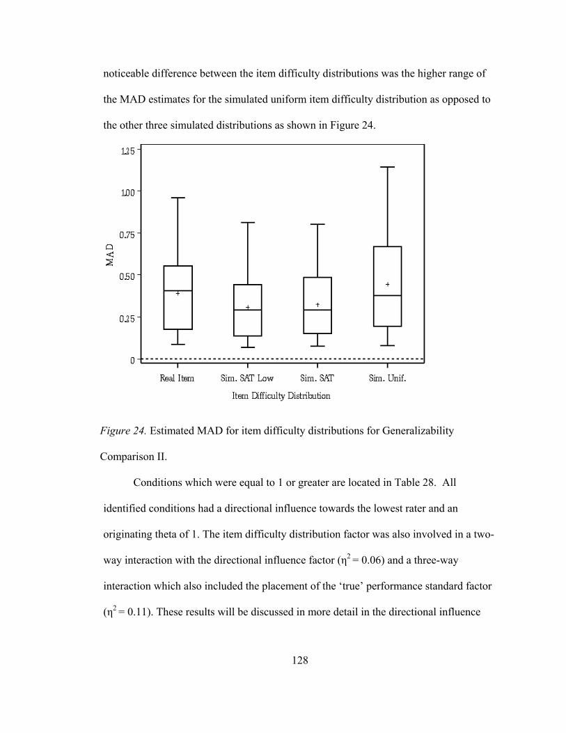
128
noticeable difference between the item difficulty distributions was the higher range of
the MAD estimates for the simulated uniform item difficulty distribution as opposed to
the other three simulated distributions as shown in Figure 24.
Figure 24. Estimated MAD for item difficulty distributions for Generalizability
Comparison II.
Conditions which were equal to 1 or greater are located in Table 28. All
identified conditions had a directional influence towards the lowest rater and an
originating theta of 1. The item difficulty distribution factor was also involved in a two-
way interaction with the directional influence factor (η2 = 0.06) and a three-way
interaction which also included the placement of the ‘true’ performance standard factor
(η2 = 0.11). These results will be discussed in more detail in the directional influence
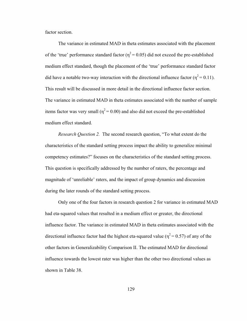
129
factor section.
The variance in estimated MAD in theta estimates associated with the placement
of the ‘true’ performance standard factor (η2 = 0.05) did not exceed the pre-established
medium effect standard, though the placement of the ‘true’ performance standard factor
did have a notable two-way interaction with the directional influence factor (η2 = 0.11).
This result will be discussed in more detail in the directional influence factor section.
The variance in estimated MAD in theta estimates associated with the number of sample
items factor was very small (η2 = 0.00) and also did not exceed the pre-established
medium effect standard.
Research Question 2. The second research question, “To what extent do the
characteristics of the standard setting process impact the ability to generalize minimal
competency estimates?” focuses on the characteristics of the standard setting process.
This question is specifically addressed by the number of raters, the percentage and
magnitude of ‘unreliable’ raters, and the impact of group dynamics and discussion
during the later rounds of the standard setting process.
Only one of the four factors in research question 2 for variance in estimated MAD
had eta-squared values that resulted in a medium effect or greater, the directional
influence factor. The variance in estimated MAD in theta estimates associated with the
directional influence factor had the highest eta-squared value (η2 = 0.57) of any of the
other factors in Generalizability Comparison II. The estimated MAD for directional
influence towards the lowest rater was higher than the other two directional values as
shown in Table 38.
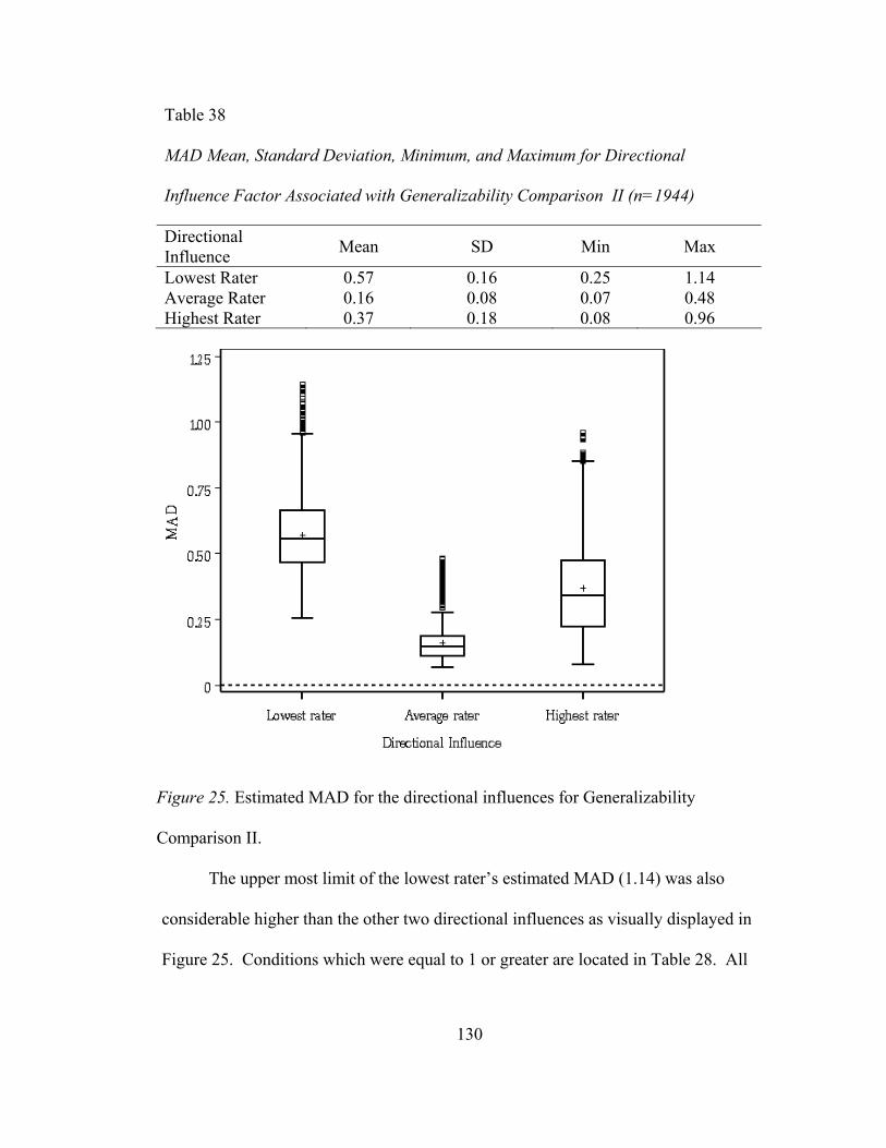
130
Table 38
MAD Mean, Standard Deviation, Minimum, and Maximum for Directional
Influence Factor Associated with Generalizability Comparison II (n=1944)
Directional Influence Mean SD Min Max
Lowest Rater 0.57 0.16 0.25 1.14 Average Rater 0.16 0.08 0.07 0.48 Highest Rater 0.37 0.18 0.08 0.96
Figure 25. Estimated MAD for the directional influences for Generalizability
Comparison II.
The upper most limit of the lowest rater’s estimated MAD (1.14) was also
considerable higher than the other two directional influences as visually displayed in
Figure 25. Conditions which were equal to 1 or greater are located in Table 28. All
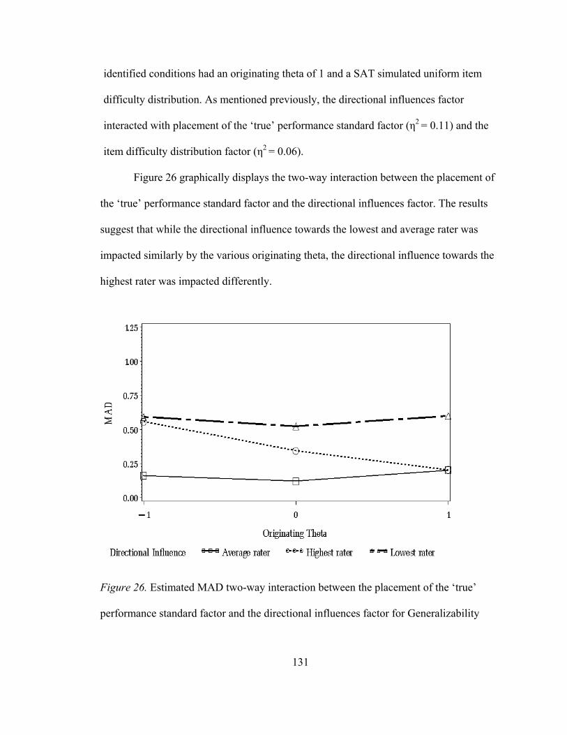
131
identified conditions had an originating theta of 1 and a SAT simulated uniform item
difficulty distribution. As mentioned previously, the directional influences factor
interacted with placement of the ‘true’ performance standard factor (η2 = 0.11) and the
item difficulty distribution factor (η2 = 0.06).
Figure 26 graphically displays the two-way interaction between the placement of
the ‘true’ performance standard factor and the directional influences factor. The results
suggest that while the directional influence towards the lowest and average rater was
impacted similarly by the various originating theta, the directional influence towards the
highest rater was impacted differently.
Figure 26. Estimated MAD two-way interaction between the placement of the ‘true’
performance standard factor and the directional influences factor for Generalizability
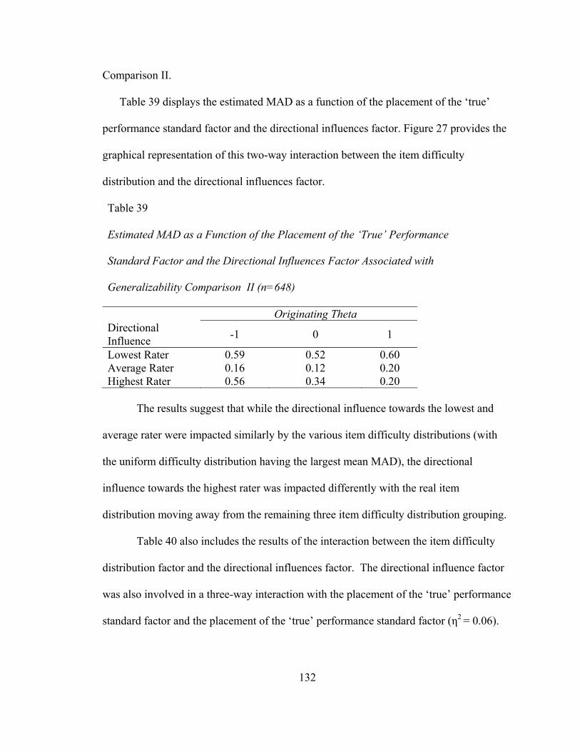
132
Comparison II.
Table 39 displays the estimated MAD as a function of the placement of the ‘true’
performance standard factor and the directional influences factor. Figure 27 provides the
graphical representation of this two-way interaction between the item difficulty
distribution and the directional influences factor.
Table 39
Estimated MAD as a Function of the Placement of the ‘True’ Performance
Standard Factor and the Directional Influences Factor Associated with
Generalizability Comparison II (n=648)
Originating Theta Directional Influence -1 0 1
Lowest Rater 0.59 0.52 0.60 Average Rater 0.16 0.12 0.20 Highest Rater 0.56 0.34 0.20
The results suggest that while the directional influence towards the lowest and
average rater were impacted similarly by the various item difficulty distributions (with
the uniform difficulty distribution having the largest mean MAD), the directional
influence towards the highest rater was impacted differently with the real item
distribution moving away from the remaining three item difficulty distribution grouping.
Table 40 also includes the results of the interaction between the item difficulty
distribution factor and the directional influences factor. The directional influence factor
was also involved in a three-way interaction with the placement of the ‘true’ performance
standard factor and the placement of the ‘true’ performance standard factor (η2 = 0.06).
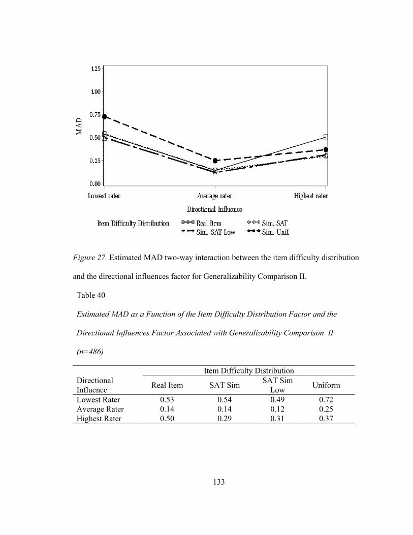
133
Figure 27. Estimated MAD two-way interaction between the item difficulty distribution
and the directional influences factor for Generalizability Comparison II.
Table 40
Estimated MAD as a Function of the Item Difficulty Distribution Factor and the
Directional Influences Factor Associated with Generalizability Comparison II
(n=486)
Item Difficulty Distribution Directional Influence Real Item SAT Sim SAT Sim
Low Uniform
Lowest Rater 0.53 0.54 0.49 0.72 Average Rater 0.14 0.14 0.12 0.25 Highest Rater 0.50 0.29 0.31 0.37
134
Figures 28-30 display the results of this three-way interaction for each level of the
originating theta. When the originating theta is -1, the four item difficulty distributions
converge in terms of mean MAD when the direction influence is to the lowest rater.
Figure 28. Estimated MAD interaction between item difficulty distribution factor and the
directional influences factor at originating theta=-1 for Generalizability Comparison II.
When the directional influence is towards the average rater, the real item and
simulated uniform distributions converge in terms of mean MAD, while the simulated
SAT and simulated SAT with lower variance distributions converge at a lower mean
MAD. The relationship between item difficulty distributions is even more pronounced
when the directional influence is towards the highest rater. When the originating theta is
0, the four item difficulty distributions have the least amount of convergence in terms of
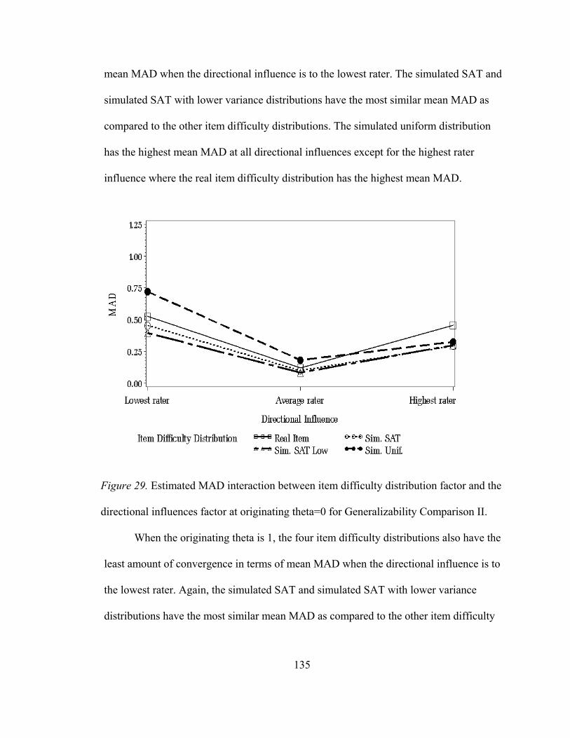
135
mean MAD when the directional influence is to the lowest rater. The simulated SAT and
simulated SAT with lower variance distributions have the most similar mean MAD as
compared to the other item difficulty distributions. The simulated uniform distribution
has the highest mean MAD at all directional influences except for the highest rater
influence where the real item difficulty distribution has the highest mean MAD.
Figure 29. Estimated MAD interaction between item difficulty distribution factor and the
directional influences factor at originating theta=0 for Generalizability Comparison II.
When the originating theta is 1, the four item difficulty distributions also have the
least amount of convergence in terms of mean MAD when the directional influence is to
the lowest rater. Again, the simulated SAT and simulated SAT with lower variance
distributions have the most similar mean MAD as compared to the other item difficulty
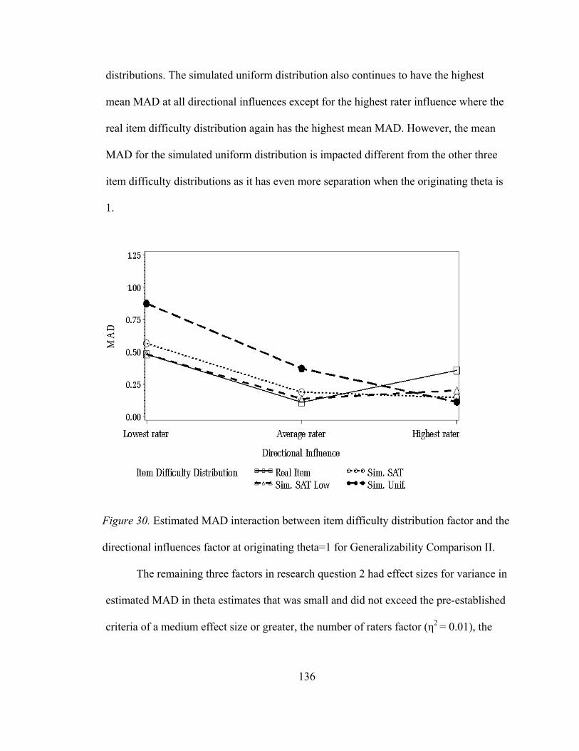
136
distributions. The simulated uniform distribution also continues to have the highest
mean MAD at all directional influences except for the highest rater influence where the
real item difficulty distribution again has the highest mean MAD. However, the mean
MAD for the simulated uniform distribution is impacted different from the other three
item difficulty distributions as it has even more separation when the originating theta is
1.
Figure 30. Estimated MAD interaction between item difficulty distribution factor and the
directional influences factor at originating theta=1 for Generalizability Comparison II.
The remaining three factors in research question 2 had effect sizes for variance in
estimated MAD in theta estimates that was small and did not exceed the pre-established
criteria of a medium effect size or greater, the number of raters factor (η2 = 0.01), the
137
percentage of unreliable raters factor (η2 = 0.02), and the magnitude of ‘unreliability’
factor (η2 = 0.02).
Actual Standard Setting Results Comparison
Results from an actual Angoff standard setting process were used as a ‘pseudo’
population. Samples were then drawn using a similar stratified random sampling
methodology and comparisons were made to the results of the simulation study.
Comparisons were made between an actual 112-item Angoff dataset (provided by S. G.
Sireci) and the simulation results. The actual Angoff dataset contained 13 raters. One
rater was randomly selected and removed in order to match the simulation parameters
for rater size. The 112-item set contained one-parameter IRT values. The mean b-
parameter was 0.01 (SD = 0.91) with a minimum value of -3.83 and a maximum value of
1.61.
The ability to generalize the performance standard was evaluated using a model
similar to that used in the simulation. Since the items were calibrated under a one-
parameter IRT model, only the difficulty parameters could be used for the stratification.
The individual item difficulty parameters (b-values) were separated into three groups
and stratified random samples were extracted based on one of the three item difficulty
groupings. This ensured representative groups of item difficulty in the drawn samples.
The sample sizes were based on the sample size factor used in the simulation. To match
the characteristics of the simulation design and ensure stable results, one thousand
samples were taken from each sample size. The three outcomes (bias, RMSE, and MAD)
were calculated for each sample size across the one thousand samples.
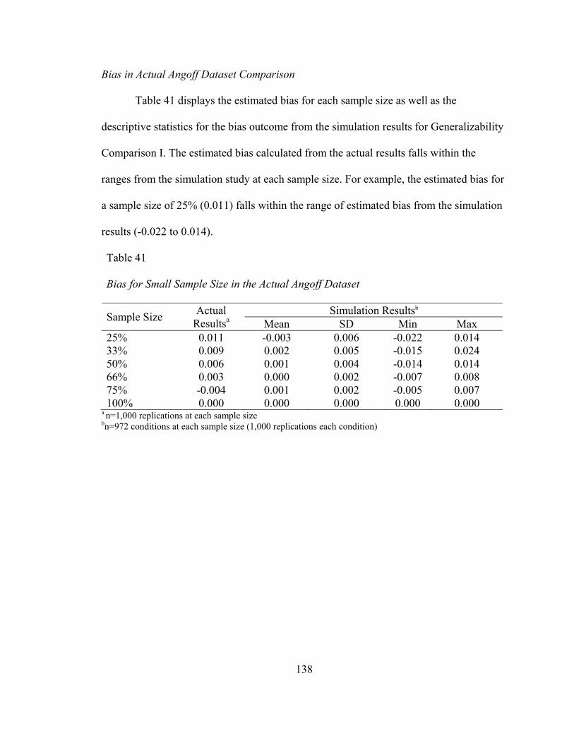
138
Bias in Actual Angoff Dataset Comparison
Table 41 displays the estimated bias for each sample size as well as the
descriptive statistics for the bias outcome from the simulation results for Generalizability
Comparison I. The estimated bias calculated from the actual results falls within the
ranges from the simulation study at each sample size. For example, the estimated bias for
a sample size of 25% (0.011) falls within the range of estimated bias from the simulation
results (-0.022 to 0.014).
Table 41
Bias for Small Sample Size in the Actual Angoff Dataset
Simulation Resultsb Sample Size Actual Resultsa Mean SD Min Max
25% 0.011 -0.003 0.006 -0.022 0.014 33% 0.009 0.002 0.005 -0.015 0.024 50% 0.006 0.001 0.004 -0.014 0.014 66% 0.003 0.000 0.002 -0.007 0.008 75% -0.004 0.001 0.002 -0.005 0.007 100% 0.000 0.000 0.000 0.000 0.000
a n=1,000 replications at each sample size
bn=972 conditions at each sample size (1,000 replications each condition)
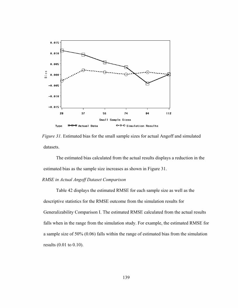
139
Figure 31. Estimated bias for the small sample sizes for actual Angoff and simulated
datasets.
The estimated bias calculated from the actual results displays a reduction in the
estimated bias as the sample size increases as shown in Figure 31.
RMSE in Actual Angoff Dataset Comparison Table 42 displays the estimated RMSE for each sample size as well as the
descriptive statistics for the RMSE outcome from the simulation results for
Generalizability Comparison I. The estimated RMSE calculated from the actual results
falls when in the range from the simulation study. For example, the estimated RMSE for
a sample size of 50% (0.06) falls within the range of estimated bias from the simulation
results (0.01 to 0.10).
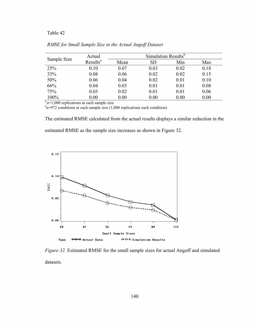
140
Table 42
RMSE for Small Sample Size in the Actual Angoff Dataset
Simulation Resultsb Sample Size Actual Resultsa Mean SD Min Max
25% 0.10 0.07 0.03 0.02 0.18 33% 0.08 0.06 0.02 0.02 0.15 50% 0.06 0.04 0.02 0.01 0.10 66% 0.04 0.03 0.01 0.01 0.08 75% 0.03 0.02 0.01 0.01 0.06 100% 0.00 0.00 0.00 0.00 0.00
a n=1,000 replications at each sample size
bn=972 conditions at each sample size (1,000 replications each condition)
The estimated RMSE calculated from the actual results displays a similar reduction in the
estimated RMSE as the sample size increases as shown in Figure 32.
Figure 32. Estimated RMSE for the small sample sizes for actual Angoff and simulated
datasets.
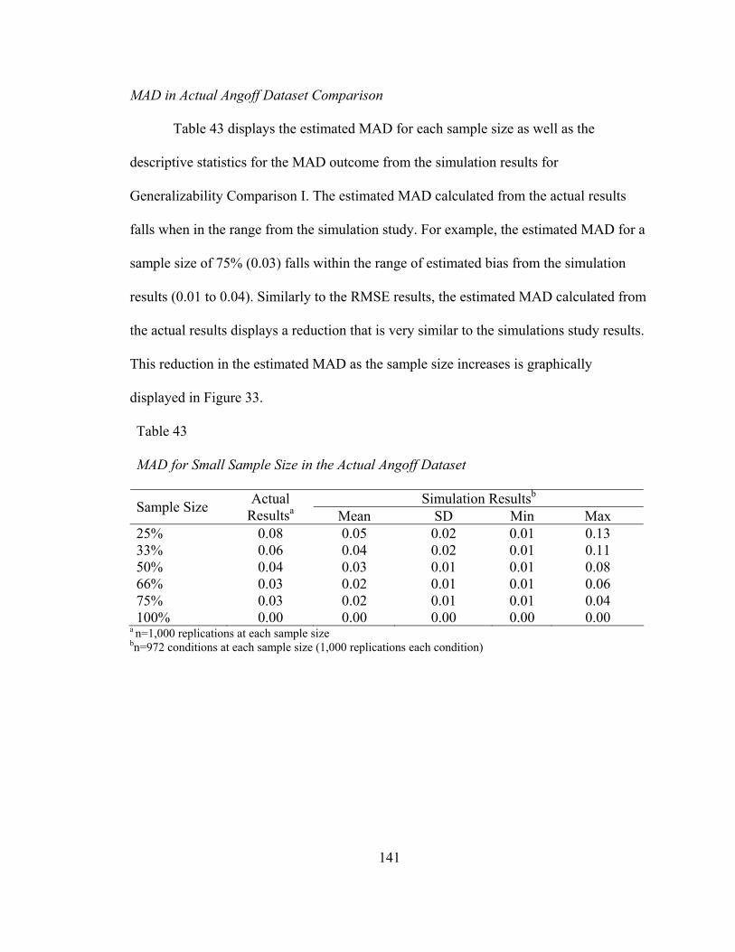
141
MAD in Actual Angoff Dataset Comparison
Table 43 displays the estimated MAD for each sample size as well as the
descriptive statistics for the MAD outcome from the simulation results for
Generalizability Comparison I. The estimated MAD calculated from the actual results
falls when in the range from the simulation study. For example, the estimated MAD for a
sample size of 75% (0.03) falls within the range of estimated bias from the simulation
results (0.01 to 0.04). Similarly to the RMSE results, the estimated MAD calculated from
the actual results displays a reduction that is very similar to the simulations study results.
This reduction in the estimated MAD as the sample size increases is graphically
displayed in Figure 33.
Table 43
MAD for Small Sample Size in the Actual Angoff Dataset
Simulation Resultsb Sample Size Actual Resultsa Mean SD Min Max
25% 0.08 0.05 0.02 0.01 0.13 33% 0.06 0.04 0.02 0.01 0.11 50% 0.04 0.03 0.01 0.01 0.08 66% 0.03 0.02 0.01 0.01 0.06 75% 0.03 0.02 0.01 0.01 0.04 100% 0.00 0.00 0.00 0.00 0.00
a n=1,000 replications at each sample size
bn=972 conditions at each sample size (1,000 replications each condition)
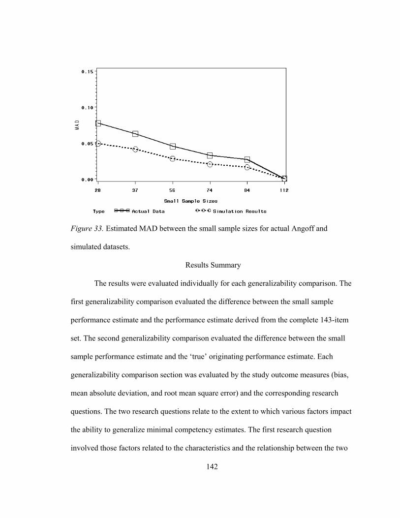
142
Figure 33. Estimated MAD between the small sample sizes for actual Angoff and
simulated datasets.
Results Summary
The results were evaluated individually for each generalizability comparison. The
first generalizability comparison evaluated the difference between the small sample
performance estimate and the performance estimate derived from the complete 143-item
set. The second generalizability comparison evaluated the difference between the small
sample performance estimate and the ‘true’ originating performance estimate. Each
generalizability comparison section was evaluated by the study outcome measures (bias,
mean absolute deviation, and root mean square error) and the corresponding research
questions. The two research questions relate to the extent to which various factors impact
the ability to generalize minimal competency estimates. The first research question
involved those factors related to the characteristics and the relationship between the two
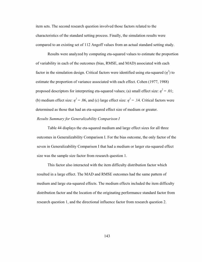
143
item sets. The second research question involved those factors related to the
characteristics of the standard setting process. Finally, the simulation results were
compared to an existing set of 112 Angoff values from an actual standard setting study.
Results were analyzed by computing eta-squared values to estimate the proportion
of variability in each of the outcomes (bias, RMSE, and MAD) associated with each
factor in the simulation design. Critical factors were identified using eta-squared (η2) to
estimate the proportion of variance associated with each effect. Cohen (1977, 1988)
proposed descriptors for interpreting eta-squared values; (a) small effect size: η2 = .01;
(b) medium effect size: η2 = .06, and (c) large effect size: η2 = .14. Critical factors were
determined as those that had an eta-squared effect size of medium or greater.
Results Summary for Generalizability Comparison I
Table 44 displays the eta-squared medium and large effect sizes for all three
outcomes in Generalizability Comparison I. For the bias outcome, the only factor of the
seven in Generalizability Comparison I that had a medium or larger eta-squared effect
size was the sample size factor from research question 1.
This factor also interacted with the item difficulty distribution factor which
resulted in a large effect. The MAD and RMSE outcomes had the same pattern of
medium and large eta-squared effects. The medium effects included the item difficulty
distribution factor and the location of the originating performance standard factor from
research question 1, and the directional influence factor from research question 2.
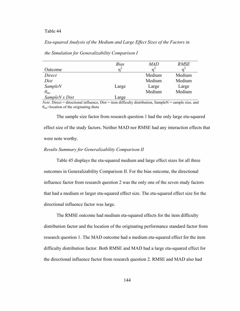
144
Table 44
Eta-squared Analysis of the Medium and Large Effect Sizes of the Factors in
the Simulation for Generalizability Comparison I
Bias MAD RMSE Outcome η2 η2 η2 Direct Medium Medium Dist Medium Medium SampleN Large Large Large θmc Medium Medium SampleN x Dist Large
Note. Direct = directional influence, Dist = item difficulty distribution, SampleN = sample size, and θmc=location of the originating theta
The sample size factor from research question 1 had the only large eta-squared
effect size of the study factors. Neither MAD nor RMSE had any interaction effects that
were note worthy.
Results Summary for Generalizability Comparison II
Table 45 displays the eta-squared medium and large effect sizes for all three
outcomes in Generalizability Comparison II. For the bias outcome, the directional
influence factor from research question 2 was the only one of the seven study factors
that had a medium or larger eta-squared effect size. The eta-squared effect size for the
directional influence factor was large.
The RMSE outcome had medium eta-squared effects for the item difficulty
distribution factor and the location of the originating performance standard factor from
research question 1. The MAD outcome had a medium eta-squared effect for the item
difficulty distribution factor. Both RMSE and MAD had a large eta-squared effect for
the directional influence factor from research question 2. RMSE and MAD also had
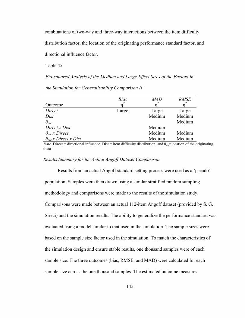
145
combinations of two-way and three-way interactions between the item difficulty
distribution factor, the location of the originating performance standard factor, and
directional influence factor.
Table 45
Eta-squared Analysis of the Medium and Large Effect Sizes of the Factors in
the Simulation for Generalizability Comparison II
Bias MAD RMSE Outcome η2 η2 η2 Direct Large Large Large Dist Medium Medium θmc Medium Direct x Dist Medium θmc x Direct Medium Medium θmc x Direct x Dist Medium Medium
Note. Direct = directional influence, Dist = item difficulty distribution, and θmc=location of the originating theta Results Summary for the Actual Angoff Dataset Comparison
Results from an actual Angoff standard setting process were used as a ‘pseudo’
population. Samples were then drawn using a similar stratified random sampling
methodology and comparisons were made to the results of the simulation study.
Comparisons were made between an actual 112-item Angoff dataset (provided by S. G.
Sireci) and the simulation results. The ability to generalize the performance standard was
evaluated using a model similar to that used in the simulation. The sample sizes were
based on the sample size factor used in the simulation. To match the characteristics of
the simulation design and ensure stable results, one thousand samples were of each
sample size. The three outcomes (bias, RMSE, and MAD) were calculated for each
sample size across the one thousand samples. The estimated outcome measures

146
calculated from the actual results all fell when in the range from the simulation study.
The outcome measures from the actual results also displayed similar reductions to the
simulation study as the samples increased in size.
147
Chapter Five:
Conclusions
Summary of the Study
While each phase of the test development process is crucial to the validity of the
examination, one phase tends to stand out among the others; the standard setting process.
It has continually received the most attention in the literature among any of the technical
issues related to criterion-referenced measurement (Berk, 1986). Little research attention,
however, has been given to generalizing the resulting performance standards. In essence,
can the estimate of minimal competency that is established with one subset of multiple
choice items be applied to the larger set of items from which it was derived? The ability
to generalize performance standards has profound implications both from a psychometric
as well as a practicality standpoint.
The standard setting process is a time-consuming and expensive endeavor. It
requires the involvement of number of professionals both in the context of participants
such as subject matter experts (SME) as well as those involved in the test development
process such as psychometricians and workshop facilitators. The standard setting process
can also be cognitively taxing on participants (Lewis et al., 1998). Generalizing
performance standards may improve the quality of the standard setting process. By
reducing the number of items that a rater needs to review, the quality of their ratings
might improve as the raters are “less fatigued” and have “more time” to review the
148
smaller dataset (Ferdous & Plake, 2005, p. 186). Reducing the time it takes to conduct
the process also translates into a savings of time and money for the presenting agency as
well as the raters, who are generally practitioners in the profession.
While IRT-based models such as the Bookmark and other variations have been
created to addresses some of these the deficiencies, research suggests that these newer
IRT-based methods have inadvertently introduced other flaws. In a multimethod study of
standard setting methodologies by Buckendahl et al. (2000), the Bookmark standard
setting method did not produce levels of confidence and comfort with the process that
were very different than the popular Angoff method. Reckase (2006a) conducted a
simulation study of standard setting processes using Angoff and Bookmark methods
which attempted to recover the originating performance standard in the simulation model.
He found that error-free conditions during the first round of Bookmark cut scores were
statistically lower than the simulated cut scores (Reckase, 2006a). The Bookmark
estimates of the performance standard from his research study were ‘uniformly
negatively statistically biased’ (Reckase, 2006a, p. 14). These results are consistent with
other Bookmark research (Green et al., 2003; Yin & Schulz, 2005). While the IRT-based
standard setting methods do use a common scale, they all have a potential issue with
reliability. Raters are only given one opportunity per round to determine an estimate of
minimal competency as they select a single place between items rather than setting
performance estimates for each individual item as in the case of the Angoff method.
Setting a performance standard with the Angoff method on a smaller sample of
items and accurately applying it to the larger test form may address some of these
149
standard setting issues (e.g., cognitively taxing process, high expense, time consuming).
In fact, it may improve the standard setting process by limiting the number of items and
the individual rater decisions. It also has the potential to save time and money as fewer
individual items would be used in the process.
The primary purpose of this research was to evaluate the extent to which a single
minimal competency estimate derived from a subset of multiple choice items would
generalize to the larger item set. There were two primary goals for this research
endeavor: (1) evaluating the degree to which the characteristics of the two item sets and
their relationship impact the ability to generalize minimal competency estimates, and (2)
evaluating the degree to which the characteristics of the standard setting process impact
the ability to generalize minimal competency estimates.
First, the characteristics and the relationship between the two item sets were
evaluated in terms of their effect on generalizability. This included the distribution of
item difficulties in the larger item set, the placement of the ‘true’ performance standard,
and the number of items randomly drawn from the larger item set. Second, the
characteristics of the standard setting process were evaluated in terms of their effect on
generalizability: specifically, elements such as the number of raters, the ‘unreliability’ of
individual raters in terms of the percentage of unreliable raters and their magnitude of
‘unreliability’, and the influence of group dynamics and discussion.
Individual item-level estimates of minimal competency were simulated using a
Monte Carlo approach. This type of approach allowed the control and manipulation of
research design factors. Every simulation study begins with various decision points.
150
These decision points represent the researcher’s attempt to ground the simulation process
in current theory and provide a foundation for the creation of ‘real life’ data and results
that can be correctly generalized to specific populations. The initial decision points
involved in this simulation are the type of standard setting method, the type of IRT
model, and the number of items evaluated. The Angoff method was selected over the
Bookmark method as the standard setting method for this study due to its popularity of
use (Ferdous & Plake, 2005), stronger ability to replicate the performance standard
(Reckase, 2006a), and greater amount of general research as well as research on the
ability to generalize performance standards. The IRT method selected was based on the
characteristics of the items. Multiple choice items were used and the three-parameter IRT
model which incorporates a pseudo guessing parameter was the most appropriate IRT
model for this type of item. The decision to use a large number of items for the larger
item set was based on the research questions. There would be less economic value in
dividing a smaller number of items into even smaller samples.
The simulation took place in two distinct steps: data generation and data analysis.
The data generation step consisted of simulating the standard setting participant’s
individual estimates of minimal competency and calculating the resulting item-level
estimates of minimal competency. The second step or data analysis step of the simulation
process consisted of forming a smaller item set by drawing a stratified random sample
from the larger item set. The resulting performance standard established with this smaller
item set was then compared to the performance standard from the larger item set as well
as the ‘true’ performance standard used to originally simulate the data. The Monte Carlo
151
study involved seven factors. The simulation factors were separated into two areas: those
related to the characteristics and relationship between the item sets, and those related to
the standard setting process. The characteristics and the relationship between the two
item sets included three factors: (a) the item difficulty distributions in the larger 143-item
set (‘real’ item distribution, simulated SAT item distribution, simulated SAT item
distribution with reduced variance, and simulated uniform difficulty), (b) location of the
‘true’ performance standard (θmc = -1.0, 0, 1.0), (c) number of items randomly drawn in
the sample (36, 47, 72, 94, 107, and the full item set). The characteristics of the standard
setting process included four factors: (a) number of raters (8, 12, 16), (b) percentage of
unreliable raters (25%, 50%, 75%), (c) magnitude of ‘unreliability’ in unreliable raters
(ρXX = .65, .75, .85.), and (d) and the directional influence of group dynamics and
discussion (lowest rater, highest rater, average rater).
The ability to ‘adequately’ generalize the performance was evaluated in terms of
the differences between the performance standard derived with the larger item set and the
performance standard derived with the smaller subset of multiple choice items. The
difference between the originating performance standard and the performance standard
derived with the smaller subset of items was also examined. The aggregated simulation
results were evaluated in terms of the location (bias) and the variability (mean absolute
deviation, root mean square error) in the estimates. The examining proportion of variance
associated with each effect (η2) was evaluated using Cohen’s medium effect size criteria,
η2 = 0.06.
152
Research Questions
1. To what extent do the characteristics and the relationship between the two item sets
impact the ability to generalize minimal competency estimates?
a. To what extent does the distribution of item difficulties in the larger item set
influence the ability to generalize the estimate of minimal competency?
b. To what extent does the placement of the ‘true’ performance standard influence
the ability to generalize the estimate of minimal competency?
c. To what extent does the number of items drawn from the larger item set
influence the ability to generalize the estimate of minimal competency?
2. To what extent do the characteristics of the standard setting process impact the ability to
generalize minimal competency estimates?
a. To what extent does the number of raters in the standard setting process
influence the ability to generalize the estimate of minimal competency?
b. To what extent does the percentage of ‘unreliable’ raters influence the ability to
generalize the estimate of minimal competency?
c. To what extent does the magnitude of ‘unreliability’ in the designated
‘unreliable’ raters influence the ability to generalize the estimate of minimal
competency?
d. To what extent do group dynamics and discussion during the later rounds of the
standard setting process influence the ability to generalize the estimate of
minimal competency?
153
Summary of Results
Generalizability Comparison I
For the bias outcome, the only factor of the seven in Generalizability Comparison
I that had a medium or larger eta-squared effect size was the sample size factor from
research question 1. This factor also interacted with the item difficulty distribution factor
which resulted in a large effect. The MAD and RMSE outcomes had the same pattern of
medium and large eta-squared effects. The medium effects included the item difficulty
distribution factor and the location of the originating performance standard factor from
research question 1, and the directional influence factor from research question 2. The
sample size factor from research question 1 had the only large eta-squared effect size of
the study factors. Neither MAD nor RMSE had any interaction effects that were note
worthy.
Generalizability Comparison II
The directional influence factor from research question 2 was the only one of the
seven study factors that had a medium or larger eta-squared effect size. The eta-squared
effect size for the directional influence factor was large. The RMSE outcome had
medium eta-squared effects for the item difficulty distribution factor and the location of
the originating performance standard factor from research question 1. The MAD
outcome had a medium eta-squared effect for the item difficulty distribution factor. Both
RMSE and MAD had a large eta-squared effect for the directional influence factor from
research question 2. RMSE and MAD also had combinations of two-way and three-way
interactions between the item difficulty distribution factor, the location of the originating

154
performance standard factor, and directional influence factor.
Actual Angoff Dataset Comparison
Results from an actual Angoff standard setting process were used as a ‘pseudo’
population. Samples were then drawn using a similar stratified random sampling
methodology and comparisons were made to the results of the simulation study.
Comparisons were made between the minimal competency estimates derived from the
simulation results and those derived from an actual 112-item Angoff dataset (provided
by S. G. Sireci). The ability to generalize the performance standard was evaluated using
a model similar to that used in the simulation. The sample sizes were based on the
sample size factor used in the simulation. To match the characteristics of the simulation
design and ensure stable results, one thousand samples were taken from each sample
size. The three outcomes (bias, RMSE, and MAD) were calculated for each sample size
across the one thousand samples. The outcome measures calculated from the actual
results were all within the range of the simulation study results. The outcome measures
from the actual results also displayed similar reductions in variance as the sample size
increased.
Discussion
Previous research studies related to using subsets of items to set performance
standards have only been conducted on existing Angoff datasets. Little or no previous
research exists evaluating the extent to which various standard setting factors impact the
generalizability of performance standards. This simulation study sought to explore these
various factors within the standard setting process and their impact on generalizability.
155
Two different generalizability comparisons were made as a result of the study. The first
generalizability comparison evaluated the difference between the small sample
performance estimate and the performance estimate derived from the complete 143-item
set. The second generalizability comparison evaluated the difference between the small
sample performance estimate and the ‘true’ originating performance estimate. Because
of the uniqueness of each of the generalizability comparisons, each will be discussed
separately as they relate to the research questions and their associated study factors and
then differences will be compared at the end of the section.
Generalizability Comparison I
Three factors were associated with the characteristics and the relationship
between the two item sets as stated in research question 1. All three factors were
postulated to impact the ability to generalize minimal competency estimates between the
small sample performance estimate and the performance estimate derived from the
complete 143-item set. These three factors were the distribution of item difficulties in
the larger item set, the placement of the ‘true’ performance standard, and the number of
items drawn from the larger item set.
It was hypothesized that item difficulty distributions with a smaller variance in
item difficulty parameters will generalize better than item difficulty distributions with a
larger variance. The study results suggest that there is some value to this hypothesis.
While little bias was present in the item difficulty factor of the simulation study, the
variability in theta estimates (RMSE and MAD) was very noticeable. The mean RMSE
(0.025) was the smallest in the simulated SAT Low item difficulty distribution (lower
156
variance in item difficulty parameters). This item difficulty distribution also had the
lowest variability in item difficulty parameters (SD = 0.70). This suggests that the tighter
the item difficulty distribution, the better the generalizability of performance estimates.
Conversely, the item difficulty distribution with the largest variability in difficulty
parameters, the simulated SAT uniform distribution (SD = 1.69), had the highest mean
RMSE (0.044) of the four item difficulty distributions.
In terms of location of the ‘true’ performance standard, it was suggested that a ‘true’
performance standard which is closer to the center of the item difficulty distribution will
generalize better than a placement further away. The simulations study results also suggest
that this hypothesis has some merit. While little bias was present in the location of the ‘true’
performance factor, the variability (RMSE and MAD) in theta estimates was very noticeable.
Of the three originating theta values, an originating theta value of 1 had the lowest mean
RMSE (0.027) and lowest range of RMSE values (0.111) of the three originating theta
values. The mean item difficulty parameters (b-parameter) for the four item difficulty
distributions were -0.01(Simulated SAT Low), -0.07 (Simulated SAT), 0.09 (Simulated SAT
Uniform), and 0.44 (Real Item). While a strong interaction between the originating theta
factor and the item difficulty distribution factor was not present, this could explain why an
originating theta of 1 had a lower mean RMSE than an originating theta of -1. An originating
theta of 0 had the second lowest mean RMSE (0.031) of the three originating theta values.
It was also suggested that the larger the number of sample items drawn from the
143-item sample the better the generalizability of the estimate of minimal competency.
This was true in the study both in terms of the bias and the variability (RMSE and MAD)
157
in theta estimates. In fact, this factor had the largest outcome measure effect sizes of the
seven study factors in Generalizability Comparison I. The results of the simulation study
suggest that the larger the sample size the less bias and variability of theta estimates. This
result is consistent with the current literature (Coraggio, 2007; Ferdous & Plake, 2005,
2007; Sireci et al., 2000). The number of sample items factor also interacted with the
item difficulty distribution factor. The ability to generalize performance estimates
increased as the sample size increased, but not at the same rate for all four item difficulty
distributions. The item difficulty distribution that was impacted the most was the SAT
Uniform distribution which interestingly also had the most variability (SD = 1.69) in item
difficulty parameters (b-parameters).
Four factors were associated with the characteristics of the standard setting
process as stated in research question 2. All four factors were postulated to impact the
ability to generalize minimal competency estimates between the small sample
performance estimate and the performance estimate derived from the complete 143-item
set. These four factors were the number of raters, the percentage of ‘unreliable’ raters,
magnitude of ‘unreliability’ in the designated ‘unreliable’ raters, and the group dynamics
and discussion during the second round of the standard setting process.
It was hypothesized that the larger the numbers of raters in the standard setting
process the better the generalizability of the estimate of minimal competency. This was
based on the literature suggesting that at least 10 and ideally 15 to 20 should participate
(Brandon, 2004). The three levels in this study were selected to be representative and at
the same time economical based on the nature of the research topic. The number of raters
158
factor in the study did not produce any notable results in terms of the bias and variability
(RMSE and MAD) of theta estimates.
It was also suggested that the consistency of raters and magnitude of consistency
would impact the generalizability of the performance estimates. While this is also
suggested in the literature (Schultz, 2006; Shepard, 1995), the results of this study did not
support this hypothesis. None of these rater related factors produced notable results in
terms of the bias and variability (theta) of theta estimates. This included the percentage of
‘unreliable’ raters and the magnitude of unreliability in the fallible raters.
The group dynamics and discussion during the second round of the standard
setting process did produce noticeable results in the study. It was suggested that group
dynamics and discussion that influence the raters towards the center of the rating
distribution would generalize better than group dynamics and discussion that influence
the raters towards the outside of the rating distribution. Fitzpatrick (1989) had suggested
that a group polarization effect that occurs during the discussion phase of the Angoff
workshop and Livingston (1995) had reported that this effect was towards the mean
rating. The results of this study suggest that the directional influence towards the highest
rater had best generalizability of theta estimates. The directional influence towards the
highest rater had the lowest mean RMSE (0.027) and lowest range of RMSE values
(0.109). While it was hypothesized that the directional influence towards the average
rater would have the best generalizability of theta estimates, the reason for the slight
advantage in the directional results towards the highest rater is not immediately apparent.
Further research on the issue of the impact of directional influence should be conducted
159
to investigate this outcome. The directional influence towards the average rater was a
very close second with a mean RMSE of 0.032.
Generalizability Comparison II
Three factors were associated with the characteristics and the relationship
between the two item sets as stated in research question 1. All three factors were
postulated to impact the ability to generalize minimal competency estimates between the
small sample performance estimate and the ‘true’ originating performance estimate.
These three factors were the distribution of item difficulties in the larger item set, the
placement of the ‘true’ performance standard, and the number of items drawn from the
larger item set.
It was hypothesized that item difficulty distributions with a smaller variance in
item difficulty parameters will generalize better than item difficulty distributions with a
larger variance. The study results suggest that this hypothesis may be accurate for
Generalizability Comparison II as well as Generalizability Comparison I. While little
bias was present in the item difficulty factor of the simulation study, the variability
(RMSE and MAD) in theta estimates was very noticeable. The mean RMSE was the
smallest (0.33) in the simulated SAT with low item difficulty variance. This item
difficulty distribution also had the lowest variability in item difficulty parameters (SD =
0.70). Conversely, the item difficulty distribution with the largest variability in difficulty
parameters, the SAT Uniform distribution (SD = 1.69), had the highest mean RMSE
(0.48). The item difficulty distribution also had two note-worthy interactions, one with
the directional influence factor, and one with the directional influence factor and the
160
originating theta factor. In both cases, the SAT Uniform distribution displayed less
generalizability of performance estimates than the other four item difficulty
distributions.
In terms of location of the ‘true’ performance standard, it was also suggested that a
placement of the ‘true’ performance standard closer to the center of the item difficulty
distribution will generalize better than a placement further away. The simulation study
results also suggest that this hypothesis has some merit. While little bias was present in the
location of the ‘true’ performance factor of the simulation study, the variability (RMSE) in
theta estimates was very noticeable. Of the three originating theta values, an originating theta
value of 0 had the lowest mean RMSE (0.36) and lowest standard deviation of RMSE (0.19)
of the three originating theta values. As mentioned earlier, there was an interaction between
the originating theta factor and the item difficulty distribution factor. The mean item
difficulty parameters (b-parameter) for the four item difficulty distributions were -
0.01(Simulated SAT Low), -0.07 (Simulated SAT), 0.09 (Simulated SAT Uniform), and 0.44
(Real Item). All four item difficulty distributions center around an originating theta of 0 with
a slight skewness towards an originating theta of 1. An originating theta of 1 had the second
lowest mean RMSE (0.39) with a standard deviation of RMSE (0.23).
Regarding the number of items drawn, it was hypothesized that the larger the
number of items drawn the better the generalizability of the estimate of minimal
competency. The results of this study did not support this hypothesis in Generalizability
Comparison II. The sample size factor did not produce any notable results in terms of the
bias and the variability (RMSE and MAD) of theta estimates. This factor was very
161
noteworthy in Generalizability Comparison I for all three outcome measures, when
comparing the generalizability between the small sample and the full 143-item set.
However, this generalizability comparison was between the small sample and the
originating or ‘true’ theta. Little research exists on the concept of a true’ theta and
researchers are only able to determine the ‘true’ originating theta in simulation studies.
Some researchers even argue the existence of a ‘true’ originating theta (Schultz, 2006;
Wang et al., 2003). One possible reason for this difference in results between the
generalizability comparisons is that other factors (such as the directional influence factor)
may have accounted for such large shares of the explained variance in the outcome
measures that they essentially drown out the impact of the sample size factor in
Generalizability Comparison II.
Four factors were associated with the characteristics of the standard setting
process as stated in research question 2. All four factors were postulated to impact the
ability to generalize minimal competency estimates between the small sample
performance estimate and the ‘true’ originating performance estimate. These four factors
were the number of raters, the percentage of ‘unreliable’ raters, the magnitude of
‘unreliability’ in the designated ‘unreliable’ raters, and the group dynamics and
discussion during the second round of the standard setting process.
It was hypothesized that the larger the numbers of raters in the standard setting
process the better the generalizability of the estimate of minimal competency. While the
literature suggested minimum and recommended levels of the number of raters (Brandon,
2004), the three levels used in this study (8, 12, and 16) did not produce any notable
162
results in terms of the bias and variability (RMSE and MAD) of theta estimates for
Generalizability Comparison II. It was also hypothesized that the consistency of raters
and magnitude of consistency would impact the generalizability of the performance
estimates. While this is also suggested in the literature (Schultz, 2006; Shepard, 1995),
the results of this study did not support this hypothesis for Generalizability Comparison
II. As with the results of the first generalizability comparison, none of the rater related
factors produced notable results in terms of the bias and variability (RMSE and MAD) of
theta estimates.
It was also suggested that group dynamics and discussion that influence the raters
towards the center of the rating distribution would generalize better than group dynamics
and discussion that influence the raters towards the outside of the rating distribution. The
simulation study results suggest that this is an accurate hypothesis as the directional
influence towards the average rater had the lowest mean bias (-0.07) and mean RMSE
(0.19). This is consistent with the rater regression to the mean effect discussed in the
literature (Livingston, 1995). Directional influence towards the lowest rater was
negatively bias (-0.57), while directional influence towards the highest rater was
positively bias (0.35). This result was different than the result for the other
generalizability comparison. This factor had the largest outcome measure effect sizes of
the seven study factors in Generalizability Comparison II.
Limitations
Based on the design of the study, there are a number of limitations to consider in
relation to this research study. The simulation method implemented in this study provides
163
control of a number of factors intended to investigate performance in specific situations.
This benefit of control in simulation studies is also a limitation as it tends to limit the
generalizability of the study findings. Thus, the seven controlled factors (a) the item
difficulty distributions, (b) location of the ‘true’ performance standard, (c) number of
items randomly drawn in the sample, (d) number of raters, (e) percentage of unreliable
raters, (f) magnitude of ‘unreliability’ in unreliable raters, and (g) directional influence of
group dynamics and discussion dictate the types of standard setting environments to
which the study results can be generalized. Another inherent limitation of the simulation
study is the number of levels within each factor. These levels were selected to provide a
sense of the impact of each factor. They were not intended to be an exhaustive
representation of all the possible levels within each factor.
Another restriction on the ability to generalize the study results is related to the
study’s initial decision points. While the researcher attempted to ground the simulation
process in current theory and provide a foundation for the creation of ‘real life’ data in
order to generalize to specific populations, the initial decision points also provided
limitations. For example, the Angoff method was selected as the standard setting model.
The use of other models such as the Bookmark method may produce very different
results. The other two decisions points of IRT method (three-parameter) and larger item
sample size (143 items) also provide similar limitations on the generalizability of study
results.
The final consideration of limited generalizability is the level of rater subjectivity
involved in the standard setting process. While this study has contained a number of
164
factors to simulate the standard setting process, additional factors affecting the
subjectiveness of individual raters such as content biases, knowledge of minimal
competency, and fatigue may also play a role in determining the final passing standard.
These issues would likely affect the other raters in the standard setting process as well.
Implications
Implications for Standard Setting Practice
The intent of this research was to evaluate the model of setting performance
standards with partial items sets. This line of research has important implications for
standard setting practice as using a subset of multiple choice items to set the passing
standard has the potential to save time and money as well as improve the quality of the
standard setting process. This could be accomplished through limiting the number of
items and the number of individual rater decisions required for the process. The quality
of individual ratings might also improve as the raters are “less fatigued” and have “more
time” to review the items (Ferdous & Plake, 2005, p. 186). Financial savings could be
redirected to improving other areas of the test development process such as validation.
This simulation research made two comparisons of generalizability. The first
addressed the differences between the performance standard derived with the larger item
set and the performance standard derived with the smaller subset of multiple choice
items. This first comparison has implications that are directly apparent for practitioners
as they generally start with the larger set of items from which to subset. The implications
for the second comparison may not be as immediately apparent, but may be just as
important. It was the difference between the ‘true’ originating performance standard and
165
the performance standard derived with the smaller subset of multiple choice items. The
‘true’ performance standard is never known in practice and some researchers have even
questioned its existence (Schultz, 2006; Wang et al., 2003). It was simulated as a factor
in this study and has direct implications in terms of the ability of a standard setting model
to reproduce the intended standard (Reckase, 2006a, 2006b).
The simulation results suggest that the model of using partial item sets may have
some merit for practitioners as the resulting performance standard estimates may
generalize to those set with the larger item set. The results for the comparison between
the large and small item sets indicate large effect sizes (η2) for the sample size factor both
in terms of bias and variability (RMSE and MAD). The results also suggest that sample
sizes between 50% and 66% of the larger item set may be adequate. The estimated mean
bias for the sample size of 50% was 0.001 (SD=0.004) with an RMSE of 0.04 (SD=0.02),
while the mean bias for the sample size of 66% was less than 0.000 (SD=0.002) with an
RMSE of 0.03 (SD=0.01). This finding is consistent with non-simulated research
(Ferdous & Plake, 2005, 2007; Sireci et al., 2000). Interestingly enough the second
generalizability comparison, which evaluated the difference between the small sample
performance estimate and the ‘true’ originating performance estimate, did not produce
any note worthy results in the outcome measures. This suggests that the smallest sample
and the largest sample generalized to the ‘true’ originating performance standard equally
as well. These results do not seem very intuitive and may require additional research.
This simulation study by design has explored the conditions that may impact the
generalizability of performance standards. Previous research studies related to using
166
subsets of items to set performance standards have only been conducted on existing
datasets. This simulation study sought to explore various factors within the standard
setting process and their specific impact on generalizability. This included characteristics
related to the item sets as well as those related to the standard setting process. In fact, the
simulation results suggest that some elements of the process should be carefully
considered before attempting to set standards with subsets of items. Elements such as the
type of the item difficulty distribution in the larger item set (or original test form); the
direction of the group influence during the group discussion phase; and the location of
the ‘true’ performance standard may adversely impact generalizability.
The simulation results suggest that the item difficulty distribution can impact the
ability to generalize performance standards. The simulation study results suggest that
item difficulty distributions with a tighter variance such as those created for certification
and licensure examinations have better generalizability of performance standards. A test
of this nature would be designed to measure a more narrow range of abilities. Ideally, an
examination or bank of items for mastery testing would consist of items with item
difficulty parameters around the performance standard (Embretson & Reise, 2000). This
would provide a maximum amount of information (or conversely a low standard error)
around the performance standard. While the specific issues of computer adaptive testing
(CAT) are outside the realm of this paper (see van der Linden & Glas, 2000 for more
detail), different item selection, scoring (i.e., ML, MAP, EAP), and termination
procedures may require a wider range of item difficulty parameters than reflected by the
SAT simulated item difficulty distribution with low variance used in this study. This item
167
difficulty distribution factor had medium effect sizes (η2) in terms of variability (RMSE
and MAD) for both generalizability comparisons. This factor also interacted with the
sample size factor in Generalizability Comparison I as well as the directional influence
factor and the location of the originating performance standard in Generalizability
Comparison II.
The simulation results also suggest that directional influence by raters during the
discussion round can impact the ability to generalize performance standards. This result
is consistent with current research. Some researchers have suggested a group-influenced
biasing effect of regression to the mean (Livingston, 1995) during group discussion.
Other researchers have suggested a group polarization effect (Fitzpatrick, 1989) in which
a moderate group position becomes more extreme in that same direction after group
interaction and discussion (Myers & Lamm, 1976). Group discussion has resulted in
lower rating variability, and this lower variability has been traditionally used by
practitioners as one measure of standard setting quality. Lower variability, however, may
not guarantee valid results (McGinty, 2005). One question that has been periodically
explored in the literature is the need for the discussion round in the standard setting
process. The impact of the directional influence towards the lowest and highest raters in
Generalizability Comparison II suggests the need to revisit this question. This directional
influence factor had medium effect sizes (η2) in terms of variability (RMSE and MAD)
for Generalizability Comparison I and large effect sizes (η2) in terms of bias and
variability (RMSE and MAD) for Generalizability Comparison II. The results suggest
that directional influence while being an important consideration in terms of generalizing
168
across item sets may have an even bigger implication in terms of the ability of the
standard setting process to replicate the intended originating performance standard. This
factor also interacted with the item difficulty distribution factor and the location of the
originating performance standard factor in Generalizability Comparison II.
In addition to the item difficulty distribution and directional influence factors, the
simulation results suggest that the location of the originating performance standard factor
may also impact the ability to generalize performance standards. The simulation study
results suggest that a ‘true’ originating performance standard which is closer to the center
of the item difficulty distribution will generalize better than a placement which is further
away. This factor had medium effect sizes (η2) in terms of variability (RMSE and/or
MAD) for both generalizability comparisons. As previously mentioned, this factor
interacted with the item difficulty distribution factor and the directional influence factor
in Generalizability Comparison II.
This issue of a ‘true’ performance standard is controversial among standard
setting researchers. One way to operationalize this concept in terms of standard setting
practice is analogize it to a ‘true’ score in test theory. Normally, one would assume that
the location of the ‘true’ performance standard for a given program would not change
over time just as ‘true’ score would not change in test theory. A practitioner could
carefully consider the location of the performance standards from previous standard
settings. The average of these previous performance standards could then be considered a
‘true’ performance standard and taken into consideration when creating new test forms
and conducting future standard settings.
169
An interesting outcome of this study was the lack of noteworthy results regarding
the number and fallibility of standard setting participants. The number of raters within the
standard setting process did not seem significant in terms of impacting the
generalizability of the performance standard. Perhaps there is some validity to Livingston
and Zieky’s (1982) suggestion that as few as five participants may be adequate to set
performance standards. The study results also suggest that truly random rater error has
little impact on the ability to generalize performance standards at least in terms of the
levels used within this simulation study. The issue of non-random rater error was not as
extensively explored in this study with the exception of the factor related to directional
influence during the discussion phase of the standard setting process.
While the findings of this study are consistent with other non-simulated
generalizability research (Ferdous & Plake, 2005, 2007; Sireci et al., 2000), questions of
policy must be explored before implementing this partial item set standard setting model
in a ‘high-stakes’ testing environment. There have been few partial item set strategies
used operationally (see NAGB, 1994 for example). Questions regarding the ‘fairness’ of
setting performance standards with only partial item sets have been raised by other
researchers (Ferdous & Plake, 2007). Hambleton suggested that performance standards
set with only partial item sets would never be acceptable under today’s environment of
increased accountability (R. Hambleton, NCME session, April 10, 2007). Other ‘high
stake’ examination models have been established using partial item sets such as computer
adaptive testing (CAT) in which examinees are only presented partial item sets before a
determination of competency. CAT models have withstood judicial legislation. CAT
170
assessment models gained ‘acceptance’ after several decades of research (Embretson &
Reise, 2000). It is hoped that this study will contribute to the current limited body of
research study on setting performance standards with partial item sets.
Suggestions for Future Research
Future research should be conducted with additional combinations of raters with
different levels of fallibility to see if these rater-related results are consistent across
studies. Another suggestion for future research is to conduct standard setting research
with other item difficulty models such as items calibrated with different IRT models
(one-parameter, two-parameter, etc.) and p-value models. It would be interesting to see if
these other models produced comparable results. Clearly, the very use of IRT is a
limitation as IRT models require substantial quantities of examinee responses in order to
calibrate items. Many smaller testing programs do not have a sufficient test incident level
(responses) required for IRT.
Further research on different types of item difficulty distributions would also be
of interest. Clearly, while there were some differences in the mean and standard deviation
of the b-parameter distributions used in this study, the slight differences impacted the
results of the study. In addition, it would be interesting to further investigate the impact
of directional rater bias. This study evaluated systematic directional influence towards
another rater. Other directional bias error models should be considered. Such as models
that allow an individual rater to be randomly influenced. For example, influenced
towards the ‘highest’ rater on one item and then influenced towards the ‘lowest’ rater on
another item. It might also be interesting to evaluate the impact of a single or group of
171
raters that had a predetermined preference towards making the final performance
standard either high or low. Lastly, it would be interesting to conduct similar studies with
other types of standard setting methods such as the Bookmark method to see if they
would produce comparable results.
Conclusions Summary
The primary purpose of this research was to evaluate the extent to which a single
minimal competency estimate derived from a subset of multiple choice items would be
generalizable to the larger item set. The limited research on the subject of generalizability
of performance standards has concentrated on evaluating existing datasets. This study
sought to add to the current body of research on the subject in two ways: 1) by examining
the issue through the use of simulation and 2) by examining factors within the standard
setting process that may impact the ability to generalize performance standards.
The simulation results suggest that the model of setting performance standards
with partial item sets may have some merit as the resulting performance standard
estimates may generalize to those set with larger item sets. This finding was consistent
with the other non-simulated research (Ferdous & Plake, 2005, 2007; Sireci et al., 2000).
The simulation results also suggest that elements such as the item difficulty distribution
in the larger item set (or original test form) and the impact of directional group influence
during the group discussion phase of the process can impact generalizability. For
example, item difficulty distributions with a tighter variance and directional influence
during the discussion phase that was towards the average rater had the most favorable
results though there was often an interaction with the location of the originating
172
performance standard.
The simulation method implemented in this study provided control of a number of
factors intended to investigate performance in specific situations. However, this benefit
of control in simulation studies can also be a limitation. The seven controlled factors and
their associated levels dictate the types of standard setting environments to which the
study results can be generalized. The study’s initial decision points selected as an attempt
to ground the simulation process in current theory also created limitations. The results of
this study can only be generalized to similar environments (Angoff standard setting
method, larger item sample sizes, and three-parameter IRT models). The final
consideration of limited generalizability is the level of rater subjectivity involved in the
standard setting process. While this study has contained a number of factors to simulate
the standard setting process, additional factors affecting the subjectiveness of individual
raters such as content biases, knowledge of minimal competency, and fatigue may also
play a role in determining the final passing standard.
The number and fallibility of standard setting participants in this study had little
impact in terms of generalizability of performance standards. Future research should be
conducted with additional combinations of raters and different levels of fallibility to see
if these results are consistent across studies. Future research should also be conducted
with other item difficulty models such as items calibrated with other IRT models (one-
parameter, two-parameter, etc.) and p-value models. This study evaluated directional
influence towards another rater. It might be interesting to evaluate the impact of a single
or group of raters that had a predetermined preference towards making the final

173
performance standard either high or low. Lastly, it would be interesting to conduct
similar studies with other types of standard setting methods (e.g., Bookmark method).
174
References
Ad Hoc Committee on Confirming Test Results (2002, March). Using the National
Assessment of Educational Progress to confirm state test results. Washington,
DC: National Assessment Governing Board.
Angoff, W. H. (1971). Scales, norms, and equivalent scores. In R. L. Thorndike (Ed.),
Educational Measurement. (pp. 508-600).Washington, DC: American Council on
Education.
Behuniak, Jr., P., Archambault, F. X., & Gable R. K. (1982). Angoff and Nedelsky
standard setting procedures: Implications for the validity of proficiency test score
interpretation. Educational and Psychological Measurement, 42, 247-255.
Bejar, I. I. (1983). Subject matter experts’ assessment of item statistics. Applied
Psychological Measurement, 7, 303-310.
Beretvas, S. N. (2004). Comparison of Bookmark difficulty locations under different item
responses models. Applied Psychological Measurement, 28(1), 25-47.
Berk, R. A. (1986). A consumer’s guide to setting performance standards on criterion-
referenced tests. Review of Educational Research, 56, 137-172.
Berk, R. A. (1995). Something old, something new, something borrowed, a lot to do.
Applied Measurement in Education, 8(1), 99-109.
Berk, R. A. (1996). Standard setting: the next generation. Applied Measurement in
Education, 9(3), 215-235.
Boursicot, K., & Roberts, T. (2006). Setting standards in professional higher education
course: Defining the concept of the minimally competent student in performance-
based assessment at the level of graduation from medical school. Higher
Education Quarterly, 60 (1), 74-90.
Bowers, J. J., & Shindoll, R. R. (1989). A comparison of Angoff, Beuk, and Hofstee
methods for setting a passing score. ACT Research Report Series. 89-2.
Brandon, P. R. (2004). Conclusions about frequently studied modified Angoff standard
setting topics. Applied Measurement in Education, 17(1), 59-88.
175
Brennan, R. J., & Lockwood, R. E. (1979, April). A comparison of two cutting score
procedures using generalizability theory. Paper presented at the annual meeting
of the National Council on Measurement in Education. San Francisco, CA.
Brennan, R. J., & Lockwood, R. E. (1980). A comparison of the Nedelsky and Angoff
cutting score procedures using generalizability theory. Applied Psychological
Measurement, 4, 219-240.
Buckendahl, C. W., Impara, J. C., Giraud, G., & Irwin, P. M. (2000, April). The
consequences of judges making advanced estimates of impact on a cut score.
Paper presented at the annual meeting of American Educational Research
Association, New Orleans, LA.
Busch, J. C. & Jaeger, R. M. (1990). Influence of type of judge, normative information,
and discussion on standards recommended for the National Teachers
Examinations. Journal of Educational Measurement, 27(2), 145-163.
Cizek, G. J. (1996). An NCME instructional module on setting passing scores.
Educational Measurement: Issues and Practice, 15(2), 20-31.
Cizek, G. J., Bunch, M. B., & Koons, H. (2004). An NCME instructional module on
setting performance standards: Contemporary methods. Educational
Measurement: Issues and Practice, 23(4), 31-50.
Chang, L. (1999). Judgmental item analysis of the Nedelsky and Angoff standard setting
methods. Applied Measurement in Education, 12, 151-165.
Cohen, J. (1977). Statistical power analysis for the behavioral sciences. New York:
Academic Press.
Cohen, J. (1988). Statistical power analysis for the behavioral sciences (2nd ed.).
Hillsdale, NJ: Lawrence Erlbaum Associates.
Coraggio, J.T. (2005, November). An IRT Model for Reducing Variance in Angoff-Based
Predictions of Performance. Paper presented at the annual meeting of the Florida
Educational Research Association, Miami, FL.
176
Coraggio, J.T. (2006, November). Exploring the Generalizability of Performance
Standards using a Monte Carlo Approach. Paper presented at the annual meeting
of the Florida Educational Research Association, Jacksonville, FL.
Coraggio, J. T. (2007, April). Exploring the Generalizability of Performance Standards:
A Monte Carlo Study. Paper presented at the annual meeting of the National
Council on Measurement in Education, Chicago, IL.
Dawber, T., Rodgers, T. R., & Carbonaro, M. (2004). Robustness of Lord’s formulas for
item difficulty and discrimination conversions between classical and item
response theory models. Paper presented at the annual meeting of American
Educational Research Association, San Diego, CA.
Demauro, G. E. (2003, April). Developing a theory of performance: A two-stage
structure for the psychology of standard setting. Paper presented at the annual
meeting of the National Council on Measurement in Education, Chicago, IL.
Embretson, S. E., & Reise, S. P. (2000). Item Response Theory for Psychologists. New
Jersey: Lawrence Erlbaum Associates, Inc.
Engelhard, Jr., G., & Cramer, S. E. (1992, April). The influences of item characteristics
on judge consistency within the context of standard-setting committees. Paper
presented at the annual meeting of American Educational Research Association,
San Francisco, CA.
Equal Employment Opportunity Commission (1978). Uniform Guidelines on Employee
Selection Procedures, 41 CFR, Part 603. The Office of Personnel Management,
U.S. Department of Justice, and U.S. Department of Labor.
Fehrmann, M. L., Woehr, D. J., & Arthur, W., Jr. (1991). The Angoff cutscore method:
The impact of frame-of-reference rater training. Educational and Psychological
Measurement, 51, 857-872.
Ferrara, S. (2006) Editorial. Educational Measurement: Issues and Practices, 25(2), 1-3.
Ferdous, A. A. (2005, April). Use of an item selection strategy to estimate passing scores
in an Angoff standard setting study. Paper presented at the annual meeting of
National Council on Measurement in Education, Montreal, Canada.
177
Ferdous, A. A., & Plake, B. S. (2005). Understanding the factors that influence decisions
of panelist in standard-setting study. Applied Measurement in Education, 18(3),
257-267.
Ferdous, A. A., & Plake, B. S. (2007). Item selection strategy for reducing the number of
items rated in an Angoff standard setting study. Educational and Psychological
Measurement, 67(2), 193-206.
Fitzpatrick, A. R. (1989). Social influences in standard setting: The effects of social
interaction on group judgments. Review of Educational Research, 59, 315-328.
Gao, F., & Chen, L. (2005). Bayesian or non-Bayesian: A comparison study of item
parameter estimation in the three-parameter logistic model. Applied Measurement
in Education, 18(4), 351-380.
Gibson, W. M., &, Weiner, J. A. (1998). Generating random parallel test forms using
CTT in a computer-based environment. Journal of Educational Measurement,
35(4), 297-310.
Giraud, G., & Impara, J. C. (2000). Making the cut: A qualitative inquiry into the setting
of cut scores on school district assessments. Paper presented at the annual
meeting of Midwest Educational Research Association, Chicago, IL.
Giraud, G., Impara, J. C., & Plake, B. S. (April, 2000). A qualitative examination of
teacher’s conception of the just competent examinee in Angoff (1971) workshops.
Paper presented at the annual meeting of American Educational Research
Association, New Orleans, LA.
Giraud, G., Impara, J. C., & Plake, B. S. (2005). Teacher’s conceptions of the target
examinee in Angoff standard setting. Applied Measurement in Education, 18(3),
223-232.
Glass, G. V. (1978). Standards and criteria. Journal of Educational Measurement, 15(4),
237-261.
Goodwin, L. D. (1999). Relations between observed item difficulty levels and Angoff
minimum passing levels for a group of borderline candidates. Applied
Measurement in Education, 12(1), 13-28.
178
Green, D. R., Trimble, C. S., & Lewis, D. M. (2003). Interpreting the results of three
different standard setting procedures. Educational Measurement: Issues and
Practice, 22(1), 22–32.
Hambleton, R. K., & Swaminathan, H. (1985). Item Response Theory: Principles and
Applications. Boston: Kluwer Nijhoff Publishing.
Hambleton, R. K., Swaminathan, H., & Rodgers, H. J. (1991). Fundamentals of Item
Response Theory. Newbury Park: Sage Publications, Inc.
Han, K. T. (2007). WinGen2: Windows software that generates IRT parameters and item
responses [computer program]. Amherst, MA: Center for Educational
Assessment, University of Massachusetts Amherst. Retrieved April 1, 2007, from
http://people.umass.edu/kha/wingen/
Harwell, M., Stone, C. A., Hsu, T., & Kirisci, L. (1996). Monte Carlo studies in item
response theory. Applied Psychological Measurement, 20, 101-125.
Heldsinger, S. A., Humphry, S. M., & Andrich, D. (October, 2005). Reporting against
standards in the 21st Century: The matter of a consistent metric. Paper presented
at the 10th Annual National Roundtable Conference, Melbourne, Australia.
Hertz, N. R., & Chinn, R. N. (2002, April). The role of deliberation style in standard
setting for licensing and certification examinations. Paper presented at the annual
meeting of National Council on Measurement in Education, New Orleans, LA.
Horn, C., Ramos, M., Blumer, I., & Maduas, G. (2000). Cut scores: Results may vary.
National Board on Educational Testing and Public Policy Monographs, 1(1).
Chestnut Hill, MA: National Board on Educational Testing and Public Policy.
Hurtz, G. M., & Auerbach, M. A. (2003). A meta-analysis of the effects of modifications
to the Angoff method on cutoff scores and judgment consensus. Educational and
Psychological Measurement, 63(4), 584-601.
Huynh, H. (2000, April). On item mappings and statistical rules for selecting binary
items for criterion-referenced interpretation and Bookmark standard settings.
Paper presented at the annual meeting of National Council on Measurement in
Education, New Orleans, LA.
179
Impara, J. C. (1995). Licensure testing: purposes, procedures, and practices. Buros-
Nebraska Series on Measurement and Testing: Buros Institute.
Impara, J. C., & Plake, B. S. (1997). Standard setting: An alternative approach. Journal
of Educational Measurement, 34(4), 353-366.
Irwin, P. M., Plake, B. S., & Impara, J. C. (2000, April). Validity of item performance
estimates from an Angoff standard setting study. Paper presented at the annual
meeting of National Council on Measurement in Education, New Orleans, LA.
Jaeger, R. M. (1982). An iterative structured judgment process for establishing standards
on competency tests: Theory and application. Educational Evaluation and Policy
Analysis, 4, 461-475.
Jaeger, R. M. (1988). Use and effect of caution indices in detecting aberrant patterns of
standard-setting judgments. Applied Measurement in Education, 1, 17-31.
Jaeger, R. M. (1989a, April). Selection of judges for standard setting: What kinds? How
many? Paper presented at the annual meeting of National Council on
Measurement in Education, San Francisco, CA.
Jaeger, R. M. (1989b). Certification of student competence. In R. L. Linn (Ed.),
Educational measurement (3rd ed., pp. 485-514).Washington DC; American
Council on Education.
Jaeger, R. M. (1991). Selection of judges for standard setting. Educational
Measurement: Issues and Practice. 10(2), 3-14.
Kane, M. T. (1987). On the use of IRT models with judgmental standard setting
procedures. Journal of Educational Measurement, 24(4), 333-345.
Kane, M. T. (1994). Validating the performance standards associated with passing scores.
Review of Educational Research, 64, 425-461.
Kane, M. T. (1995). Examinee-centered vs. task-centered standard setting. Proceedings
of Joint Conference in Standard Setting for Large-Scale assessments:
Washington, DC.
180
Kane, M. T. (2001). So much remains the same: Conception and status of validation in
setting standards. In G. Cizek (Ed.), Setting performance standards: Concepts,
methods, and perspectives (pp 53-58). Mahwah, NJ: Erlbaum.
Kane, M. T., & Wilson, J. (1984). Errors of measurement and standard setting in mastery
testing. Applied Psychological Measurement, 8(1), 107-115.
Karantonis, A., & Sireci, S. G. (2006). The bookmark standard-setting method: A
literature review. Educational Measurement: Issues and Practice, 25(1), 4-12.
Lee, G., & Lewis, D. M. (2001, April). A generalizability theory approach toward
estimating standard error of cut scores set using the Bookmark standard setting
procedures. Paper presented at the annual meeting of National Council on
Measurement in Education, Seattle, WA.
Lewis, D. M. (1997). Overview of the standard errors associated with standard setting.
Unpublished manuscript. (Available from D. M. Lewis, CTB/McGraw-Hill, 20
Ryan Ranch Road, Monterey, CA 93940)
Lewis, D. M., Green, D. R., Mitzel, H. C., Baum, K., & Patz, R. J. (1998, April). The
Bookmark standard setting procedure: Methodology and recent implementations.
Paper presented at the annual meeting of the National Council for Measurement
in Education, San Diego, CA.
Lewis, D. M., Mitzel, H. C., & Green, D. R. (1996). Standard setting: A Bookmark
approach. Symposium presented at the Council of Chief State School Officers
National Conference on Large Scale Assessment, Phoenix, AZ.
Livingston, S. A. (1995). Standards for reporting the educational achievement of groups.
Proceedings of the joint committee on standard setting for large-scale
assessments of the National Assessment Governing Board (NAGB) and the
National Center for Educational Statistics (NCES).(pp. 39-51) Volume II.
Washington, DC: National Assessment Governing Board and the National Center
for Educational Statistics.
181
Livingston, S. A., & Zieky, M. J. (1982). Passing scores: A manual for setting standards
of performance on educational and occupational test. Princeton, NJ: Educational
Testing Service.
Lord, M.F. (1980). Applications of item response theory to practical testing problems.
Hillsdale NJ: Erlbaum.
Lorge, I., & Kruglov, L. K. (1953). The improvement of estimates of test difficulty.
Educational and Psychological Measurement, 13, 34-46.
McGinty, D. (2005). Illuminating the “black box” of standard setting: An exploratory
qualitative study. Applied Measurement in Education, 18(3), 269-287.
Mattar, J. D. (2000). Investigation of the validity of the Angoff standard setting
procedure for multiple choice items. Unpublished doctoral dissertation,
University of Massachusetts, Amherst, MA.
Maxwell, S. E., & Delaney, H. D. (1990). Designing experiments and analyzing data.
Belmont, CA: Wadsworth.
Mehrens, W. A. (1995). Methodological issues in standard setting for educational exams.
In Proceedings of Joint Conference on Standard setting for Large Scale
Assessments (pp 221-263). Washington, DC: National Assessment Governing
Board and National Center for Educational Statistics.
Mehrens, W. A. & Popham, W. J. (1992). How to evaluate the legal defensibility of high-
stakes tests. Applied Measurement in Education, 5(3), 265-283.
Mills, C. N., & Melican, G. J. (1988). Estimating and adjusting cutoff scores: Future of
selected methods. Applied Measurement in Education, 1, 261-275.
Mills, C. N., Melican, G. J., & Ahluwalia, N. T. (1991). Defining minimal competence.
Educational Measurement: Issues and Practice, 10(2), 7-10.
Mitzel, H. C., Lewis, D. M., Patz, R. J., & Green, D. R. (2001). The Bookmark
procedure: Psychological perspectives. In G. Cizek (Ed.), Setting performance
standards: Concepts, methods and perspectives (pp. 249-281). Mahwah, NJ:
Erlbaum.
182
Muijtjens, A. M., Kramer, A. W., Kaufman, D. M., & Van der Vleuten, C. P. (2003).
Using resampling to estimate the precision of an empirical standard-setting
method. Applied Measurement in Education, 16(3), 245-256.
Myers, D. G., & Lamm, H. (1976). The group polarization phenomenon. Psychological
Bulletin, 83(4), 602-627.
National Academy of Education. (1993). Setting performance standards for student
achievement. Stanford, CA: Author.
National Assessment Governing Board. (1994). Setting achievement levels on the 1994
National Assessment of Educational Progress in Geography and in US History
and the 1996 National Assessment of Educational Progress in Science. Final
Version. Washington, DC: Author.
Nedelsky, L. (1954). Absolute grading standards for objective tests. Educational and
Psychological Measurement, 14, 3-19.
No Child Left Behind Act of 2001, Pub. L. No. 107-110, 115 Stat.1425 (2002).
Pellegrino, J. W., Jones, L. R., & Mitchell, K. J. (1999). Grading the nation’s report
card. Washington, DC; National Academy Press.
Perie, M. (2005, April). Angoff and Bookmark methods. Paper presented at the annual
meeting of National Council on Measurement in Education, Montreal, Canada.
Plake, B. S. (1998). Setting performance standards for professional licensure and
certification. Applied Measurement in Education, 10(1), 39-59.
Plake, B. S. & Impara, J. C. (2001).Ability of panelists to estimate item performance for
a target group of candidates: An issue in judgmental standard setting. Educational
Assessment, 7(2), 87-97.
Plake, B. S., Melican, G. J., & Mills, C. N. (1991). Factors influencing intrajudge
consistency during standard setting. Educational Measurement: Issues and
Practice, 10(2), 15-25.
183
Reckase, M. D. (2000, April). The ACT/NAGB standard setting process: How "modified"
does it have to be before it is no longer a modified-Angoff process? Paper
presented at the annual meeting of the American Educational Research
Association, New Orleans, LA.
Reckase, M. D. (2005, April). A theoretical evaluation of an item rating method and a
Bookmark method for setting standards. Paper presented at the annual meeting of
the National Council on Measurement in Education, Montreal, Quebec.
Reckase, M. D. (2006a). A conceptual framework for a psychometric theory for standard
setting with examples of its use for evaluating the functioning of two standard
setting methods. Educational Measurement: Issues and Practices, 25(2), 4-18.
Reckase, M. D. (2006b). Rejoinder: Evaluating standard setting methods using error
models proposed by Schultz. Educational Measurement: Issues and Practices,
25(3), 14-17.
Reid, J. B. (1985, April). Establishing upper limits for item ratings for the Angoff
method: Are resulting standards more realistic? Paper presented at the annual
meeting of the National Council on Measurement in Education, Chicago, IL.
Reid, J. B. (1991). Training judges to generate standard-setting data. Educational
Measurement: Issues and Practices, 10(2), 11-14.
Robey, R. R. & Barcikowski, R. S. (1992). Type I error and the number of iterations in
Monte Carlo studies of robustness. British Journal of Mathematical and
Statistical Psychology, 45, 283-288.
Sato, T. (1975). The construction and interpretation of S-P tables. Tokyo: Meiji Tosho.
Schultz, E. M. (2006). Commentary: A response to Reckase’s conceptual framework and
examples for evaluating standard setting methods. Educational Measurement:
Issues and Practices, 25(3), 14-17.
Schultz, E. M., & Mitzel, H. C. (2005). The Mapmark standard setting method. Online
Submission to ERIC: Portions of this paper presented to the National Assessment
Governing Board for the National Assessment of Educational Progress.
184
Shepard, L. A. (1995). Implications for standard setting of the national academy of
education evaluation of the national assessment of educational progress
achievement levels. In Proceedings of the Joint Conference on Standard Setting
for Large Scale Assessments (pp.143-160).Washington, DC: The National
Assessment Governing Board (NAGB) and the National Center for Educational
Statistics (NCES).
Shepard, L. A., Glaser, R., Linn, R., & Bohrnstedt, G. (1993). Setting performance
standards for student achievement tests. Stanford, CA: National Academy of
Education.
Sireci, S. G., Patelis, T., Rizavi, S, Dillingham, A. M., & Rodriguez, G. (2000, April).
Setting standards on a computerized-adaptive placement examination. Paper
presented at the annual meeting of the National Council on Measurement in
Education, New Orleans, LA.
Skorupski, W. P., & Hambleton, R. K. (2005). What are panelist thinking when they
participate in standard-setting studies? Applied Measurement in Education, 18(3),
233-256.
Smith, R. L., & Smith, J. K. (1988). Differential use of item information by judges using
Angoff and Nedelsky procedures. Journal of Educational Measurement, 25(4),
259-274.
Smith, R. W., & Ferdous, A. A. (April, 2007). Using a subset of items for a modified
Angoff standard setting study: An item selection procedure. Paper presented at
the annual meeting of the National Council on Measurement in Education,
Chicago, IL.
Stark, S., Chernyshenko, O. S., & Drasgow, F. (2004). Examining the effects of
differential item (functioning and differential) test functioning on selection
decisions: When are statistically significant effects practically important? Journal
of Applied Psychology, 89(3), 497-508.
185
Swanson, D. B., Dillon, G. F., & Ross, L. E. (1990). Setting content-based standards for
national board exams: Initial research for the Comprehensive Part I Examinations.
Academic Medicine, 65, s17-s18.
Taube, K.T. (1997). The incorporation of empirical item difficulty data into the Angoff
standard-setting procedure. Evaluation & the Health Professions, 20, 479-498.
van der Linden, W. J. (1982). A latent trait method for determining intrajudge
inconsistency in the Angoff and Nedelsky techniques of standard setting. Journal
of Educational Measurement, 4, 295-305.
van der Linden, W. J. (1995). A conceptual analysis of standard setting in large scale
assessments. In L. Croker & Zieky (Eds.), Proceedings of the Joint Conference on
Standard Setting for Large Scale Assessments (Vol. 2, pp. 97-118). Washington,
DC: U.S. Government Printing Office.
van der Linden, W. J., & Glas, C. A. W. (Eds.) (2000). Computerized Adaptive Testing:
Theory and Practice. The Netherlands: Kluwer.
Wainer, H., Bradlow, E. T., & Du, Z. (2000). Testlet response theory: An analog for the
3PL model and useful in testlet-based adaptive testing. In W. J. van der Linden &
C. A. W. Glas (Eds.), Computerized adaptive testing: Theory and Practice (pp.
245-269). The Netherlands: Kluwer.
Wang, L., Pan, W., & Austin, J. T. (2003, April). Standards-setting procedures in
accountability research: Impacts of conceptual frameworks and mapping
procedures on passing rates. Paper presented at the annual meeting of the
American Educational Research Association, Chicago, IL.
Wang, X., Bradlow, E. T., & Wainer, H. (2002). A general Bayesian model for testlets:
Theory and applications. Applied Psychological Measurement, 26(1), 109-128.
Wang, N., Wiser, R. F., & Newman, L. S. (2001, April). Use of the Rasch IRT model in
standard setting: an item mapping method. Paper presented at the annual meeting
of the American Educational Research Association, Seattle, WA.
186
Wiley, A., & Guille, R. (2002, April). The occasion effect for “at-home” Angoff ratings.
Paper presented at the annual meeting of the National Council on Measurement in
Education, New Orleans, LA.
Williams, N. J., & Schultz, E. M. (2005, April). An investigation of response probability
(RP) values used in standard setting. Paper presented at the annual meeting of the
National Council on Measurement in Education, Montreal, Canada.
Yin, P., & Schultz, E. M. (2005, April). A comparison of cut scores and cut score
variability from Angoff-based and Bookmark-based procedures in standard
setting. Paper presented at the annual meeting of the National Council on
Measurement in Education, Montreal, Canada.
Zieky, M. J. (1995). A historical perspective on setting standards. In L. Crocker & M.
Zieky (Eds.), Proceedings of the Joint Conference on Standard Setting for Large
Scale Assessments (Vol. 2, pp. 1-37). Washington, DC: U. S. Government
Printing Office.
Zieky, M. J. (2001). So much has changed: How the setting of cut scores has evolved
since the 1980’s. In G. L. Cizek (Ed.), Setting performance standards: Concepts,
methods, and perspectives (pp. 19-51). Mahwah, NJ: Erlbaum.

187
Appendices
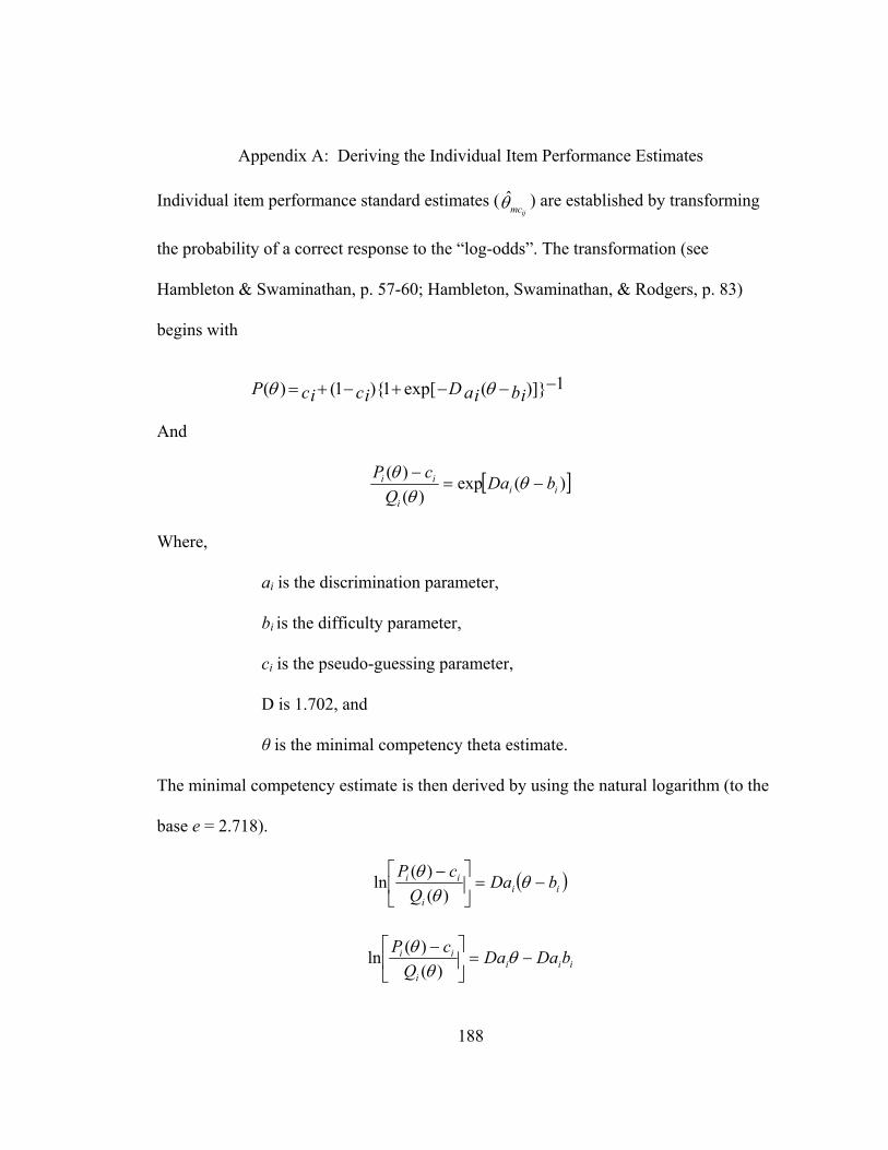
188
Appendix A: Deriving the Individual Item Performance Estimates
Individual item performance standard estimates ( ˆijmcθ ) are established by transforming
the probability of a correct response to the “log-odds”. The transformation (see
Hambleton & Swaminathan, p. 57-60; Hambleton, Swaminathan, & Rodgers, p. 83)
begins with
And
[ ])(exp)(
)(ii
i
ii bDaQ
cP−=
− θθ
θ
Where,
ai is the discrimination parameter,
bi is the difficulty parameter,
ci is the pseudo-guessing parameter,
D is 1.702, and
θ is the minimal competency theta estimate.
The minimal competency estimate is then derived by using the natural logarithm (to the
base e = 2.718).
( )iii
ii bDaQ
cP−=⎥
⎦
⎤⎢⎣
⎡ − θθ
θ)(
)(ln
iiii
ii bDaDaQ
cP−=⎥
⎦
⎤⎢⎣
⎡ − θθ
θ)(
)(ln
1)]}(exp[1){1()( −−−+−+= biaiDciciP θθ
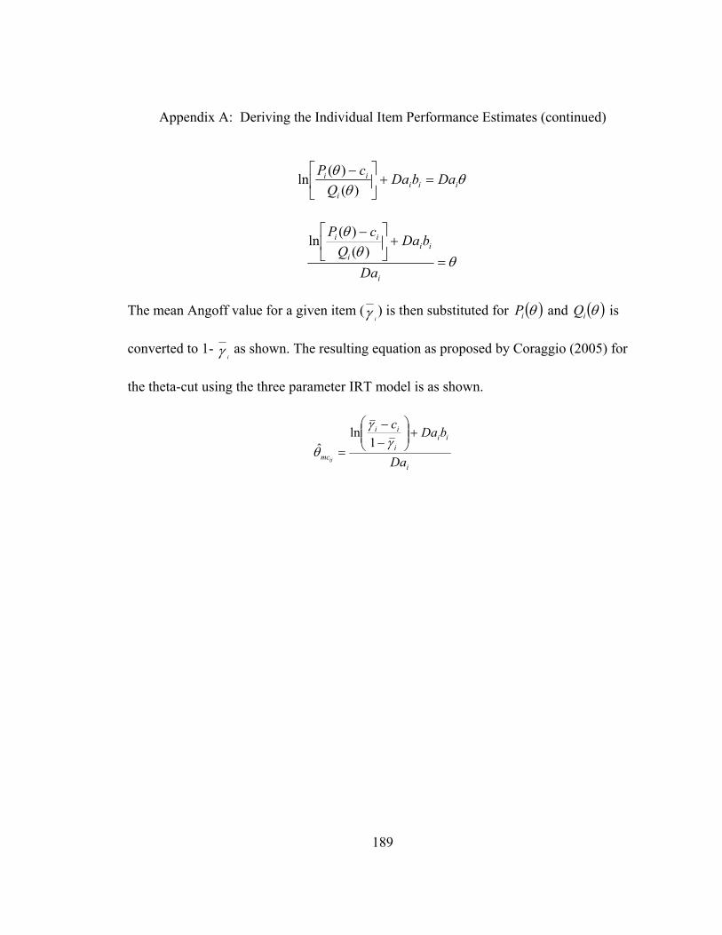
Appendix A: Deriving the Individual Item Performance Estimates (continued)
189
θθ
θiii
i
ii DabDaQ
cP=+⎥
⎦
⎤⎢⎣
⎡ −)(
)(ln
θθ
θ
=+⎥
⎦
⎤⎢⎣
⎡ −
i
iii
ii
Da
bDaQ
cP)(
)(ln
The mean Angoff value for a given item (iγ ) is then substituted for ( )θiP and ( )θiQ is
converted to 1- iγ as shown. The resulting equation as proposed by Coraggio (2005) for
the theta-cut using the three parameter IRT model is as shown.
i
iii
ii
mc Da
bDac
ij
+⎟⎟⎠
⎞⎜⎜⎝
⎛−−
=γ
γ
θ1
lnˆ
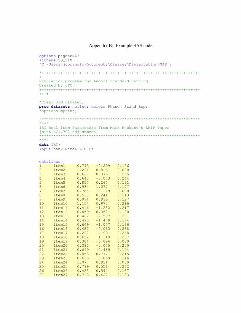
Appendix B: Example SAS code
options pageno=1; libname SS_SIM 'C:\Users\jcoraggio\Documents\Classes\Dissertation\SAS'; *++++++++++++++++++++++++++++++++++++++++++++++++++++++++++++++++++++ Simulation program for Angoff Standard Setting Created by JTC +++++++++++++++++++++++++++++++++++++++++++++++++++++++++++++++++++++++; *Clear Old dataset; proc datasets nolist; delete Phase4_Stand_Rep; *options mprint; /*********************************************************************** IRT Real Item Parameters from Mark Reckase's EMIP Paper [With A/1.702 adjustment] ***********************************************************************/ data IRT; Input bank Name$ A B C; datalines ; 1 item1 0.743 -0.299 0.186 2 item2 1.224 0.816 0.000 3 item3 0.617 0.376 0.255 4 item4 0.643 -0.003 0.244 5 item5 0.857 0.267 0.191 6 item6 0.934 1.077 0.127 7 item7 0.788 -0.149 0.000 8 item8 0.518 0.241 0.213 9 item9 0.894 0.939 0.127 10 item10 1.154 0.977 0.216 11 item11 0.416 -1.232 0.217 12 item12 0.459 0.352 0.180 13 item13 0.462 -2.597 0.201 14 item14 0.495 -1.470 0.164 15 item15 0.669 -1.047 0.186 16 item16 0.457 -0.063 0.238 17 item17 0.222 1.199 0.248 18 item18 0.652 -1.119 0.207 19 item19 0.304 -0.096 0.000 20 item20 0.335 -0.045 0.270 21 item21 0.699 -0.469 0.194 22 item22 0.853 0.777 0.215 23 item23 0.635 -0.069 0.246 24 item24 1.077 0.914 0.000 25 item25 0.799 0.556 0.202 26 item26 0.435 0.594 0.187 27 item27 0.713 0.427 0.133
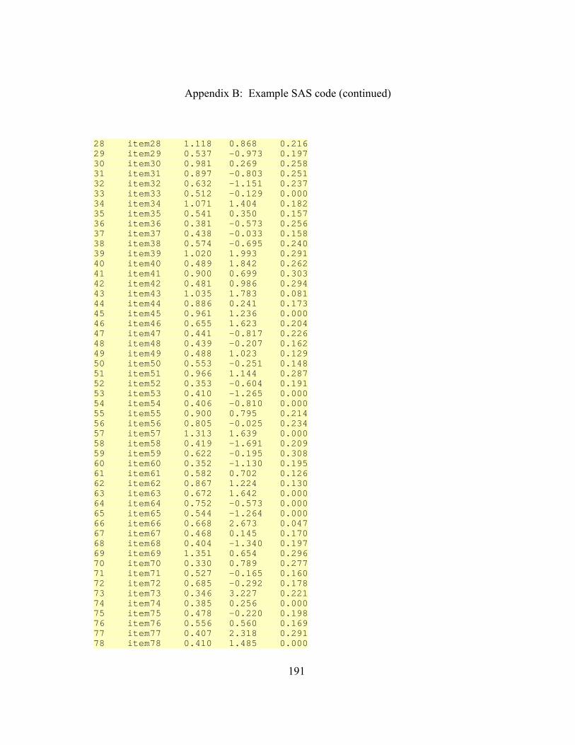
Appendix B: Example SAS code (continued)
191
28 item28 1.118 0.868 0.216 29 item29 0.537 -0.973 0.197 30 item30 0.981 0.269 0.258 31 item31 0.897 -0.803 0.251 32 item32 0.632 -1.151 0.237 33 item33 0.512 -0.129 0.000 34 item34 1.071 1.404 0.182 35 item35 0.541 0.350 0.157 36 item36 0.381 -0.573 0.256 37 item37 0.438 -0.033 0.158 38 item38 0.574 -0.695 0.240 39 item39 1.020 1.993 0.291 40 item40 0.489 1.842 0.262 41 item41 0.900 0.699 0.303 42 item42 0.481 0.986 0.294 43 item43 1.035 1.783 0.081 44 item44 0.886 0.241 0.173 45 item45 0.961 1.236 0.000 46 item46 0.655 1.623 0.204 47 item47 0.441 -0.817 0.226 48 item48 0.439 -0.207 0.162 49 item49 0.488 1.023 0.129 50 item50 0.553 -0.251 0.148 51 item51 0.966 1.144 0.287 52 item52 0.353 -0.604 0.191 53 item53 0.410 -1.265 0.000 54 item54 0.406 -0.810 0.000 55 item55 0.900 0.795 0.214 56 item56 0.805 -0.025 0.234 57 item57 1.313 1.639 0.000 58 item58 0.419 -1.691 0.209 59 item59 0.622 -0.195 0.308 60 item60 0.352 -1.130 0.195 61 item61 0.582 0.702 0.126 62 item62 0.867 1.224 0.130 63 item63 0.672 1.642 0.000 64 item64 0.752 -0.573 0.000 65 item65 0.544 -1.264 0.000 66 item66 0.668 2.673 0.047 67 item67 0.468 0.145 0.170 68 item68 0.404 -1.340 0.197 69 item69 1.351 0.654 0.296 70 item70 0.330 0.789 0.277 71 item71 0.527 -0.165 0.160 72 item72 0.685 -0.292 0.178 73 item73 0.346 3.227 0.221 74 item74 0.385 0.256 0.000 75 item75 0.478 -0.220 0.198 76 item76 0.556 0.560 0.169 77 item77 0.407 2.318 0.291 78 item78 0.410 1.485 0.000
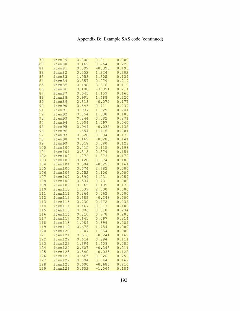
Appendix B: Example SAS code (continued)
192
79 item79 0.808 0.811 0.000 80 item80 0.462 0.264 0.223 81 item81 0.392 -0.320 0.195 82 item82 0.252 1.224 0.202 83 item83 1.058 1.305 0.134 84 item84 0.357 0.079 0.219 85 item85 0.498 3.316 0.110 86 item86 0.108 -3.851 0.211 87 item87 0.645 1.159 0.165 88 item88 0.991 1.488 0.220 89 item89 0.518 -0.072 0.177 90 item90 0.543 0.711 0.239 91 item91 0.937 1.829 0.241 92 item92 0.854 1.588 0.106 93 item93 0.844 0.582 0.271 94 item94 1.004 1.597 0.040 95 item95 0.944 -0.035 0.132 96 item96 1.554 1.416 0.201 97 item97 0.528 0.994 0.172 98 item98 0.462 -0.280 0.141 99 item99 0.518 0.580 0.123 100 item100 0.415 0.115 0.198 101 item101 0.513 0.379 0.151 102 item102 1.272 1.373 0.170 103 item103 0.428 0.674 0.186 104 item104 0.504 -0.250 0.161 105 item105 0.674 2.782 0.000 106 item106 0.752 2.100 0.000 107 item107 0.599 1.231 0.259 108 item108 0.534 0.731 0.000 109 item109 0.765 1.495 0.176 110 item110 1.039 2.000 0.000 111 item111 0.864 0.062 0.000 112 item112 0.585 -0.343 0.000 113 item113 0.730 0.472 0.232 114 item114 0.467 0.013 0.180 115 item115 0.906 0.310 0.234 116 item116 0.810 0.978 0.206 117 item117 0.641 0.597 0.314 118 item118 1.084 0.899 0.089 119 item119 0.675 1.754 0.000 120 item120 1.047 1.854 0.000 121 item121 0.616 -0.241 0.162 122 item122 0.614 0.894 0.111 123 item123 1.694 1.409 0.085 124 item124 0.607 -0.293 0.211 125 item125 0.540 -0.035 0.122 126 item126 0.565 0.226 0.256 127 item127 0.394 0.544 0.169 128 item128 0.600 -0.688 0.210 129 item129 0.602 -1.065 0.184
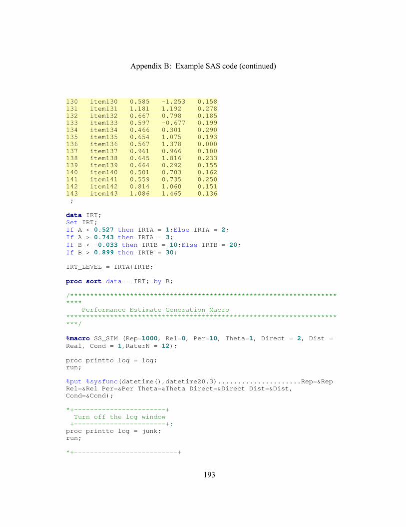
Appendix B: Example SAS code (continued)
193
130 item130 0.585 -1.253 0.158 131 item131 1.181 1.192 0.278 132 item132 0.667 0.798 0.185 133 item133 0.597 -0.677 0.199 134 item134 0.466 0.301 0.290 135 item135 0.654 1.075 0.193 136 item136 0.567 1.378 0.000 137 item137 0.961 0.966 0.100 138 item138 0.645 1.816 0.233 139 item139 0.664 0.292 0.155 140 item140 0.501 0.703 0.162 141 item141 0.559 0.735 0.250 142 item142 0.814 1.060 0.151 143 item143 1.086 1.465 0.136 ; data IRT; Set IRT; If A < 0.527 then IRTA = 1;Else IRTA = 2; If A > 0.743 then IRTA = 3; If B < -0.033 then IRTB = 10;Else IRTB = 20; If B > 0.899 then IRTB = 30; IRT_LEVEL = IRTA+IRTB; proc sort data = IRT; by B; /*********************************************************************** Performance Estimate Generation Macro ***********************************************************************/ %macro SS_SIM (Rep=1000, Rel=0, Per=10, Theta=1, Direct = 2, Dist = Real, Cond = 1,RaterN = 12); proc printto log = log; run; %put %sysfunc(datetime(),datetime20.3).....................Rep=&Rep Rel=&Rel Per=&Per Theta=&Theta Direct=&Direct Dist=&Dist, Cond=&Cond); *+-----------------------+ Turn off the log window +-----------------------+; proc printto log = junk; run; *+--------------------------+
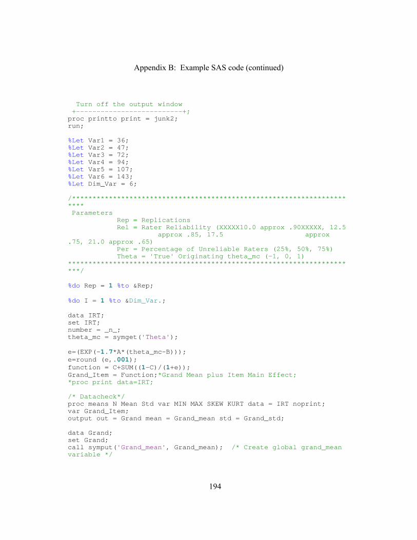
Appendix B: Example SAS code (continued)
194
Turn off the output window +--------------------------+; proc printto print = junk2; run; %Let Var1 = 36; %Let Var2 = 47; %Let Var3 = 72; %Let Var4 = 94; %Let Var5 = 107; %Let Var6 = 143; %Let Dim_Var = 6; /*********************************************************************** Parameters Rep = Replications Rel = Rater Reliability (XXXXX10.0 approx .90XXXXX, 12.5 approx .85, 17.5 approx .75, 21.0 approx .65) Per = Percentage of Unreliable Raters (25%, 50%, 75%) Theta = 'True' Originating theta_mc (-1, 0, 1) ***********************************************************************/ %do Rep = 1 %to &Rep; %do I = 1 %to &Dim_Var.; data IRT; set IRT; number = _n_; theta_mc = symget('Theta'); e=(EXP(-1.7*A*(theta_mc-B))); e=round (e,.001); function = C+SUM((1-C)/(1+e)); Grand_Item = Function;*Grand Mean plus Item Main Effect; *proc print data=IRT; /* Datacheck*/ proc means N Mean Std var MIN MAX SKEW KURT data = IRT noprint; var Grand_Item; output out = Grand mean = Grand_mean std = Grand_std; data Grand; set Grand; call symput('Grand_mean', Grand_mean); /* Create global grand_mean variable */
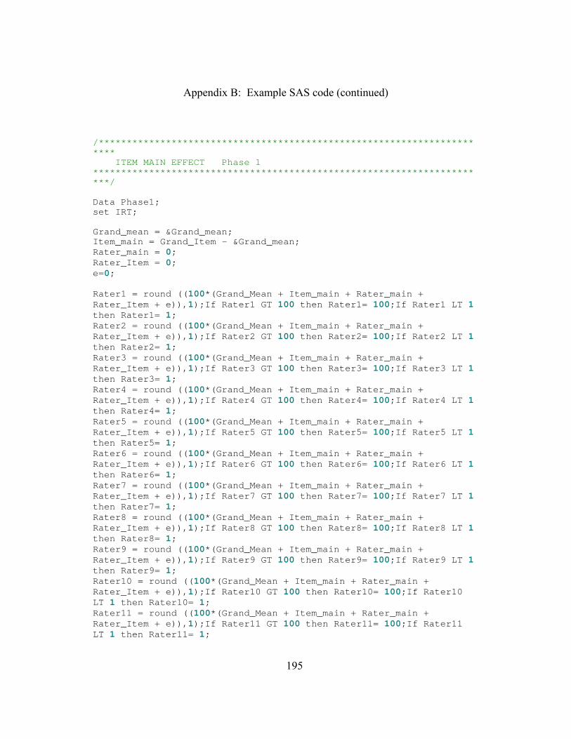
Appendix B: Example SAS code (continued)
195
/*********************************************************************** ITEM MAIN EFFECT Phase 1 ***********************************************************************/ Data Phase1; set IRT; Grand_mean = &Grand_mean; Item_main = Grand_Item - &Grand_mean; Rater_main = 0; Rater_Item = 0; e=0; Rater1 = round ((100*(Grand_Mean + Item_main + Rater_main + Rater_Item + e)),1);If Rater1 GT 100 then Rater1= 100;If Rater1 LT 1 then Rater1= 1; Rater2 = round ((100*(Grand_Mean + Item_main + Rater_main + Rater_Item + e)),1);If Rater2 GT 100 then Rater2= 100;If Rater2 LT 1 then Rater2= 1; Rater3 = round ((100*(Grand_Mean + Item_main + Rater_main + Rater_Item + e)),1);If Rater3 GT 100 then Rater3= 100;If Rater3 LT 1 then Rater3= 1; Rater4 = round ((100*(Grand_Mean + Item_main + Rater_main + Rater_Item + e)),1);If Rater4 GT 100 then Rater4= 100;If Rater4 LT 1 then Rater4= 1; Rater5 = round ((100*(Grand_Mean + Item_main + Rater_main + Rater_Item + e)),1);If Rater5 GT 100 then Rater5= 100;If Rater5 LT 1 then Rater5= 1; Rater6 = round ((100*(Grand_Mean + Item_main + Rater_main + Rater_Item + e)),1);If Rater6 GT 100 then Rater6= 100;If Rater6 LT 1 then Rater6= 1; Rater7 = round ((100*(Grand_Mean + Item_main + Rater_main + Rater_Item + e)),1);If Rater7 GT 100 then Rater7= 100;If Rater7 LT 1 then Rater7= 1; Rater8 = round ((100*(Grand_Mean + Item_main + Rater_main + Rater_Item + e)),1);If Rater8 GT 100 then Rater8= 100;If Rater8 LT 1 then Rater8= 1; Rater9 = round ((100*(Grand_Mean + Item_main + Rater_main + Rater_Item + e)),1);If Rater9 GT 100 then Rater9= 100;If Rater9 LT 1 then Rater9= 1; Rater10 = round ((100*(Grand_Mean + Item_main + Rater_main + Rater_Item + e)),1);If Rater10 GT 100 then Rater10= 100;If Rater10 LT 1 then Rater10= 1; Rater11 = round ((100*(Grand_Mean + Item_main + Rater_main + Rater_Item + e)),1);If Rater11 GT 100 then Rater11= 100;If Rater11 LT 1 then Rater11= 1;
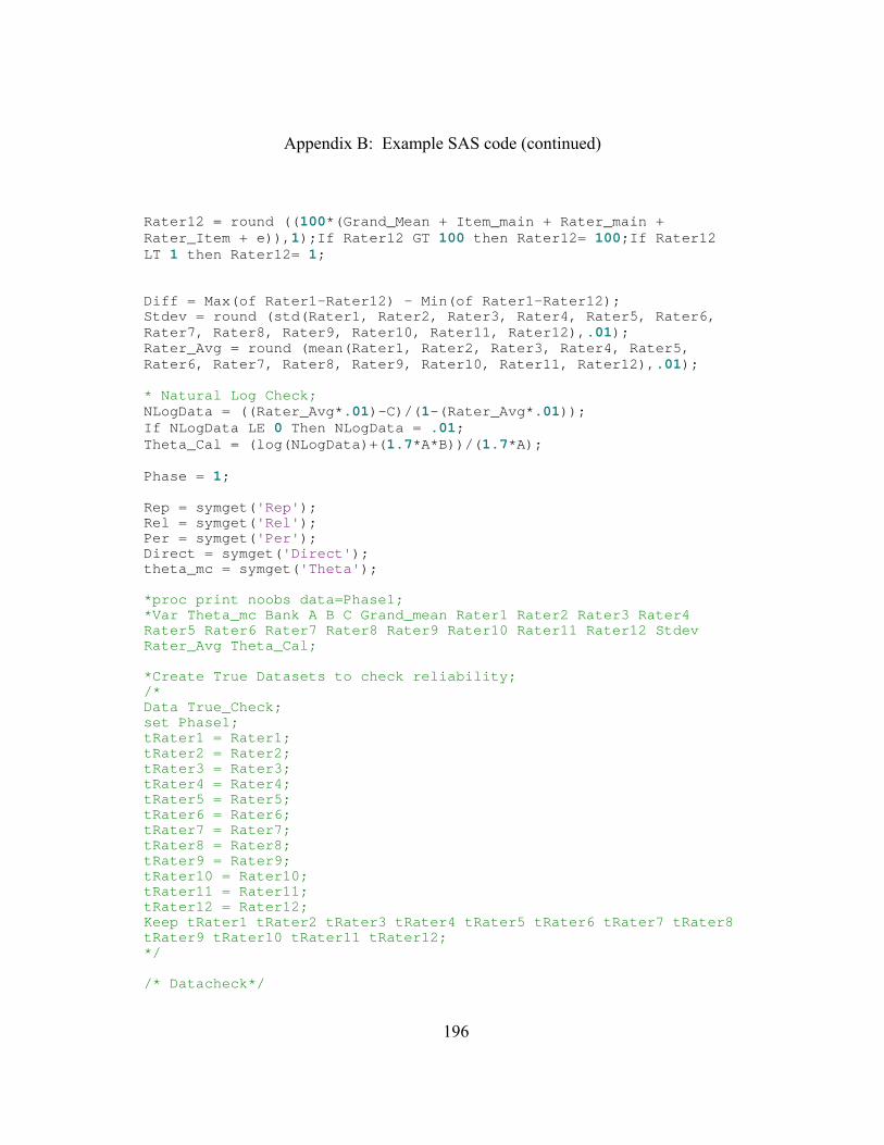
Appendix B: Example SAS code (continued)
196
Rater12 = round ((100*(Grand_Mean + Item_main + Rater_main + Rater_Item + e)),1);If Rater12 GT 100 then Rater12= 100;If Rater12 LT 1 then Rater12= 1; Diff = Max(of Rater1-Rater12) - Min(of Rater1-Rater12); Stdev = round (std(Rater1, Rater2, Rater3, Rater4, Rater5, Rater6, Rater7, Rater8, Rater9, Rater10, Rater11, Rater12),.01); Rater_Avg = round (mean(Rater1, Rater2, Rater3, Rater4, Rater5, Rater6, Rater7, Rater8, Rater9, Rater10, Rater11, Rater12),.01); * Natural Log Check; NLogData = ((Rater_Avg*.01)-C)/(1-(Rater_Avg*.01)); If NLogData LE 0 Then NLogData = .01; Theta_Cal = (log(NLogData)+(1.7*A*B))/(1.7*A); Phase = 1; Rep = symget('Rep'); Rel = symget('Rel'); Per = symget('Per'); Direct = symget('Direct'); theta_mc = symget('Theta'); *proc print noobs data=Phase1; *Var Theta_mc Bank A B C Grand_mean Rater1 Rater2 Rater3 Rater4 Rater5 Rater6 Rater7 Rater8 Rater9 Rater10 Rater11 Rater12 Stdev Rater_Avg Theta_Cal; *Create True Datasets to check reliability; /* Data True_Check; set Phase1; tRater1 = Rater1; tRater2 = Rater2; tRater3 = Rater3; tRater4 = Rater4; tRater5 = Rater5; tRater6 = Rater6; tRater7 = Rater7; tRater8 = Rater8; tRater9 = Rater9; tRater10 = Rater10; tRater11 = Rater11; tRater12 = Rater12; Keep tRater1 tRater2 tRater3 tRater4 tRater5 tRater6 tRater7 tRater8 tRater9 tRater10 tRater11 tRater12; */ /* Datacheck*/
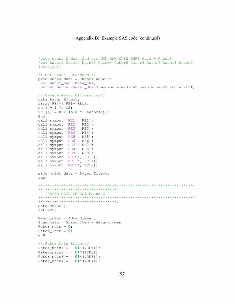
Appendix B: Example SAS code (continued)
197
*proc means N Mean Std var MIN MAX SKEW KURT data = Phase1; *var Rater1 Rater2 Rater3 Rater4 Rater5 Rater6 Rater7 Rater8 Rater9 Theta_cal; /* Get Phase1 Standard */ proc means data = Phase1 noprint; var Rater_Avg Theta_cal; output out = Phase1_Stand median = medianT mean = meanT std = stdT; /* Create Rater Differences*/ data Rater_Effect; array RE[*] RE1- RE12; do I = 1 To 12; RE [I] = 0 + (6.8 * rannor(0)); End; call symput('RE1', RE1); call symput('RE2', RE2); call symput('RE3', RE3); call symput('RE4', RE4); call symput('RE5', RE5); call symput('RE6', RE6); call symput('RE7', RE7); call symput('RE8', RE8); call symput('RE9', RE9); call symput('RE10', RE10); call symput('RE11', RE11); call symput('RE12', RE12); proc print data = Rater_Effect; run; /***************************************************************************************************** RATER MAIN EFFECT Phase 2 ******************************************************************************************************/ Data Phase2; set IRT; Grand_mean = &Grand_mean; Item_main = Grand_Item - &Grand_mean; Rater_main = 0; Rater_Item = 0; e=0; /* Rater Main Effect*/ Rater_main1 = (.01*(&RE1)); Rater_main2 = (.01*(&RE2)); Rater_main3 = (.01*(&RE3)); Rater_main4 = (.01*(&RE4));
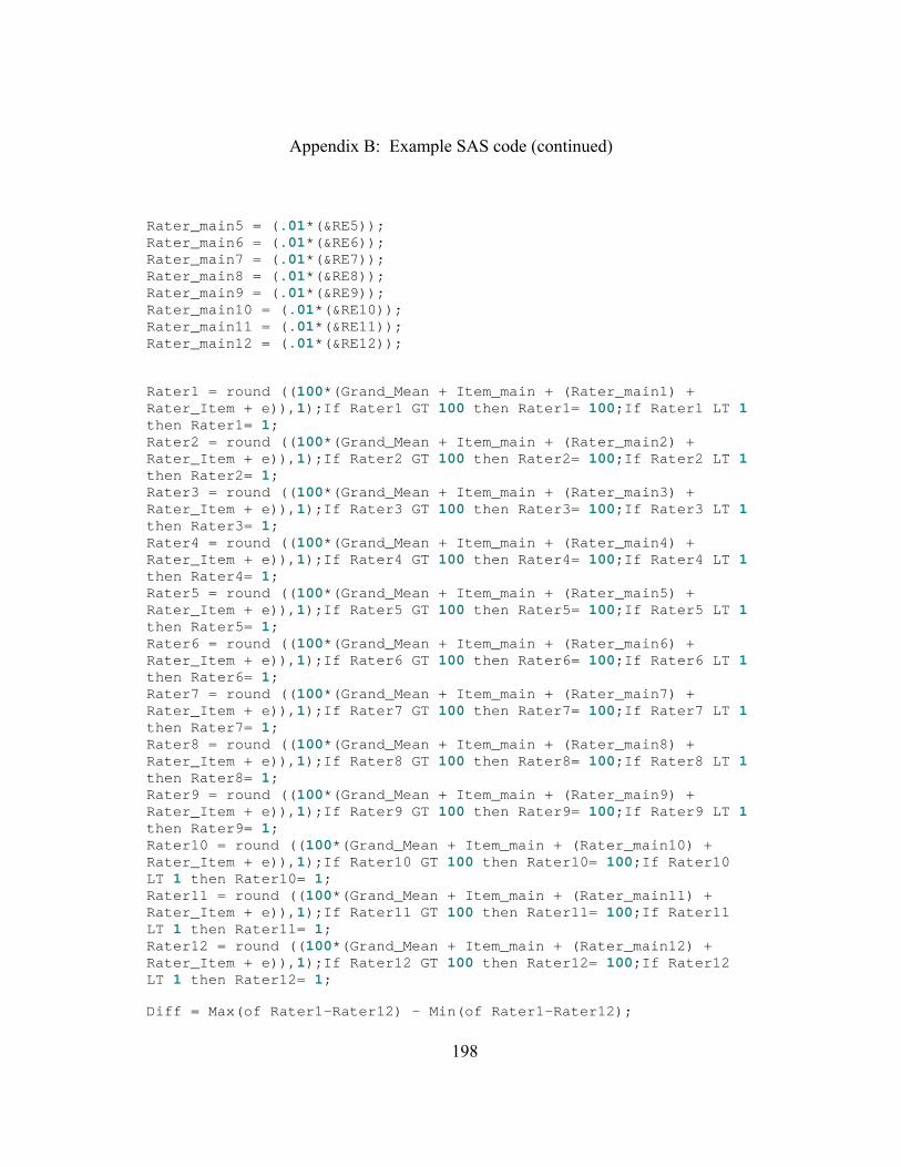
Appendix B: Example SAS code (continued)
198
Rater_main5 = (.01*(&RE5)); Rater_main6 = (.01*(&RE6)); Rater_main7 = (.01*(&RE7)); Rater_main8 = (.01*(&RE8)); Rater_main9 = (.01*(&RE9)); Rater_main10 = (.01*(&RE10)); Rater_main11 = (.01*(&RE11)); Rater_main12 = (.01*(&RE12)); Rater1 = round ((100*(Grand_Mean + Item_main + (Rater_main1) + Rater_Item + e)),1);If Rater1 GT 100 then Rater1= 100;If Rater1 LT 1 then Rater1= 1; Rater2 = round ((100*(Grand_Mean + Item_main + (Rater_main2) + Rater_Item + e)),1);If Rater2 GT 100 then Rater2= 100;If Rater2 LT 1 then Rater2= 1; Rater3 = round ((100*(Grand_Mean + Item_main + (Rater_main3) + Rater_Item + e)),1);If Rater3 GT 100 then Rater3= 100;If Rater3 LT 1 then Rater3= 1; Rater4 = round ((100*(Grand_Mean + Item_main + (Rater_main4) + Rater_Item + e)),1);If Rater4 GT 100 then Rater4= 100;If Rater4 LT 1 then Rater4= 1; Rater5 = round ((100*(Grand_Mean + Item_main + (Rater_main5) + Rater_Item + e)),1);If Rater5 GT 100 then Rater5= 100;If Rater5 LT 1 then Rater5= 1; Rater6 = round ((100*(Grand_Mean + Item_main + (Rater_main6) + Rater_Item + e)),1);If Rater6 GT 100 then Rater6= 100;If Rater6 LT 1 then Rater6= 1; Rater7 = round ((100*(Grand_Mean + Item_main + (Rater_main7) + Rater_Item + e)),1);If Rater7 GT 100 then Rater7= 100;If Rater7 LT 1 then Rater7= 1; Rater8 = round ((100*(Grand_Mean + Item_main + (Rater_main8) + Rater_Item + e)),1);If Rater8 GT 100 then Rater8= 100;If Rater8 LT 1 then Rater8= 1; Rater9 = round ((100*(Grand_Mean + Item_main + (Rater_main9) + Rater_Item + e)),1);If Rater9 GT 100 then Rater9= 100;If Rater9 LT 1 then Rater9= 1; Rater10 = round ((100*(Grand_Mean + Item_main + (Rater_main10) + Rater_Item + e)),1);If Rater10 GT 100 then Rater10= 100;If Rater10 LT 1 then Rater10= 1; Rater11 = round ((100*(Grand_Mean + Item_main + (Rater_main11) + Rater_Item + e)),1);If Rater11 GT 100 then Rater11= 100;If Rater11 LT 1 then Rater11= 1; Rater12 = round ((100*(Grand_Mean + Item_main + (Rater_main12) + Rater_Item + e)),1);If Rater12 GT 100 then Rater12= 100;If Rater12 LT 1 then Rater12= 1; Diff = Max(of Rater1-Rater12) - Min(of Rater1-Rater12);
Appendix B: Example SAS code (continued)
199
Stdev = round (std(Rater1, Rater2, Rater3, Rater4, Rater5, Rater6, Rater7, Rater8, Rater9, Rater10, Rater11, Rater12),.01); Rater_Avg = round (mean(Rater1, Rater2, Rater3, Rater4, Rater5, Rater6, Rater7, Rater8, Rater9, Rater10, Rater11, Rater12),.01); * Natural Log Check; NLogData = ((Rater_Avg*.01)-C)/(1-(Rater_Avg*.01)); If NLogData LE 0 Then NLogData = .01; Theta_Cal = (log(NLogData)+(1.7*A*B))/(1.7*A); Phase = 2; Rep = symget('Rep'); Rel = symget('Rel'); Per = symget('Per'); Direct = symget('Direct'); theta_mc = symget('Theta'); /* Datacheck proc means N Mean Std var MIN MAX SKEW KURT data = Phase2 ; var Rater1 Rater2 Rater3 Rater4 Rater5 Rater6 Rater7 Rater8 Rater9 Theta_cal; */ *proc print noobs data=Phase2; *Var Theta_mc Bank A B C Grand_mean Rater1 Rater2 Rater3 Rater4 Rater5 Rater6 Rater7 Rater8 Rater9 Rater10 Rater11 Rater12 Rater_Avg Stdev Theta_Cal Diff; /***************************************************************************************************** RATER X ITEM INTERACTION EFFECT Phase 3 ******************************************************************************************************/ Data Phase3; set IRT; Grand_mean = &Grand_mean; Item_main = Grand_Item - &Grand_mean; Rater_main = 0; Rater_Item = 0; e=0; /* Rater Main Effect */ Rater_main1 = (.01*(&RE1)); Rater_main2 = (.01*(&RE2)); Rater_main3 = (.01*(&RE3)); Rater_main4 = (.01*(&RE4)); Rater_main5 = (.01*(&RE5));
Appendix B: Example SAS code (continued)
200
Rater_main6 = (.01*(&RE6)); Rater_main7 = (.01*(&RE7)); Rater_main8 = (.01*(&RE8)); Rater_main9 = (.01*(&RE9)); Rater_main10 = (.01*(&RE10)); Rater_main11 = (.01*(&RE11)); Rater_main12 = (.01*(&RE12)); Rel = symget('Rel'); /* Rater X Item Interaction 1 Error */ Err_mean = 0; Err_SD = 6.4;****************************************Sim; I = 0; Array Ran_Err[*] Err1 - Err12; Do I = 1 To 12; Ran_Err [I] = (.01*(Err_mean + (Err_SD * rannor(0)))); End; Err_mean = 0; Err_SD2 = Rel;***************************************Sim; Per = symget('Per'); If Per = 25 then do; Err3 = (.01*(Err_mean + (Err_SD2 * rannor(0)))); Err6 = (.01*(Err_mean + (Err_SD2 * rannor(0)))); Err9 = (.01*(Err_mean + (Err_SD2 * rannor(0)))); end; If Per = 50 then do; Err1 = (.01*(Err_mean + (Err_SD2 * rannor(0)))); Err3 = (.01*(Err_mean + (Err_SD2 * rannor(0)))); Err5 = (.01*(Err_mean + (Err_SD2 * rannor(0)))); Err7 = (.01*(Err_mean + (Err_SD2 * rannor(0)))); Err9 = (.01*(Err_mean + (Err_SD2 * rannor(0)))); Err11 =(.01*(Err_mean + (Err_SD2 * rannor(0)))); end; If Per = 75 then do; Err1 = (.01*(Err_mean + (Err_SD2 * rannor(0)))); Err2 = (.01*(Err_mean + (Err_SD2 * rannor(0)))); Err4 = (.01*(Err_mean + (Err_SD2 * rannor(0)))); Err5 = (.01*(Err_mean + (Err_SD2 * rannor(0)))); Err7 = (.01*(Err_mean + (Err_SD2 * rannor(0)))); Err8 = (.01*(Err_mean + (Err_SD2 * rannor(0)))); Err10 = (.01*(Err_mean + (Err_SD2 * rannor(0)))); Err11 = (.01*(Err_mean + (Err_SD2 * rannor(0))));
Appendix B: Example SAS code (continued)
201
Err12 = (.01*(Err_mean + (Err_SD2 * rannor(0)))); end; *RI_Err = .01 * (Err_mean + (Err_SD2 * rannor(0))); Rater1 = round ((100*(Grand_Mean + Item_main + (Rater_main1) + (Rater_Item + Err1 + e))),1);If Rater1 GT 100 then Rater1= 100;If Rater1 LT 1 then Rater1= 1; Rater2 = round ((100*(Grand_Mean + Item_main + (Rater_main2) + (Rater_Item + Err2 + e))),1);If Rater2 GT 100 then Rater2= 100;If Rater2 LT 1 then Rater2= 1; Rater3 = round ((100*(Grand_Mean + Item_main + (Rater_main3) + (Rater_Item + Err3 + e))),1);If Rater3 GT 100 then Rater3= 100;If Rater3 LT 1 then Rater3= 1; Rater4 = round ((100*(Grand_Mean + Item_main + (Rater_main4) + (Rater_Item + Err4 + e))),1);If Rater4 GT 100 then Rater4= 100;If Rater4 LT 1 then Rater4= 1; Rater5 = round ((100*(Grand_Mean + Item_main + (Rater_main5) + (Rater_Item + Err5 + e))),1);If Rater5 GT 100 then Rater5= 100;If Rater5 LT 1 then Rater5= 1; Rater6 = round ((100*(Grand_Mean + Item_main + (Rater_main6) + (Rater_Item + Err6 + e))),1);If Rater6 GT 100 then Rater6= 100;If Rater6 LT 1 then Rater6= 1; Rater7 = round ((100*(Grand_Mean + Item_main + (Rater_main7) + (Rater_Item + Err7 + e))),1);If Rater7 GT 100 then Rater7= 100;If Rater7 LT 1 then Rater7= 1; Rater8 = round ((100*(Grand_Mean + Item_main + (Rater_main8) + (Rater_Item + Err8 + e))),1);If Rater8 GT 100 then Rater8= 100;If Rater8 LT 1 then Rater8= 1; Rater9 = round ((100*(Grand_Mean + Item_main + (Rater_main9) + (Rater_Item + Err9 + e))),1);If Rater9 GT 100 then Rater9= 100;If Rater9 LT 1 then Rater9= 1; Rater10 = round ((100*(Grand_Mean + Item_main + (Rater_main10) + (Rater_Item + Err10 + e))),1);If Rater10 GT 100 then Rater10= 100;If Rater10 LT 1 then Rater10= 1; Rater11 = round ((100*(Grand_Mean + Item_main + (Rater_main11) + (Rater_Item + Err11 + e))),1);If Rater11 GT 100 then Rater11= 100;If Rater11 LT 1 then Rater11= 1; Rater12 = round ((100*(Grand_Mean + Item_main + (Rater_main12) + (Rater_Item + Err12 + e))),1);If Rater12 GT 100 then Rater12= 100;If Rater12 LT 1 then Rater12= 1; Diff = Max(of Rater1-Rater12) - Min(of Rater1-Rater12); Stdev = round (std(Rater1, Rater2, Rater3, Rater4, Rater5, Rater6, Rater7, Rater8, Rater9, Rater10, Rater11, Rater12),.01); Rater_Avg = round (mean(Rater1, Rater2, Rater3, Rater4, Rater5, Rater6, Rater7, Rater8, Rater9, Rater10, Rater11, Rater12),.01);
Appendix B: Example SAS code (continued)
202
* Natural Log Check; NLogData = ((Rater_Avg*.01)-C)/(1-(Rater_Avg*.01)); If NLogData LE 0 Then NLogData = .01; Theta_Cal = (log(NLogData)+(1.7*A*B))/(1.7*A); Phase = 3; Rep = symget('Rep'); Direct = symget('Direct'); theta_mc = symget('Theta'); /***************************************************************************************************** Group Dynamics EFFECT Phase 4 ******************************************************************************************************/ /* Create Rater Influence Factor*/ data Influence_Factors; array RI[*] RI1- RI12; do I = 1 To 12; RI [I] = 0.7 + (0.1 * rannor(0)); End; call symput('RI1', RI1); call symput('RI2', RI2); call symput('RI3', RI3); call symput('RI4', RI4); call symput('RI5', RI5); call symput('RI6', RI6); call symput('RI7', RI7); call symput('RI8', RI8); call symput('RI9', RI9); call symput('RI10', RI10); call symput('RI11', RI11); call symput('RI12', RI12); Data Phase4; set Phase3; RMIN=min(of rater1-rater12); RMAX=max(of rater1-rater12); RMEAN=mean(of rater1-rater12); Direct = symget('Direct'); If Direct = 1 then XX=RMIN; If Direct = 2 then XX=RMEAN; If Direct = 3 then XX=RMAX; influ1 = (&RI1);
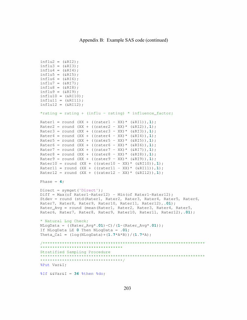
Appendix B: Example SAS code (continued)
203
influ2 = (&RI2); influ3 = (&RI3); influ4 = (&RI4); influ5 = (&RI5); influ6 = (&RI6); influ7 = (&RI7); influ8 = (&RI8); influ9 = (&RI9); influ10 = (&RI10); influ11 = (&RI11); influ12 = (&RI12); *rating = rating + (influ - rating) * influence_factor; Rater1 = round (XX + ((rater1 - XX)* (&RI1)),1); Rater2 = round (XX + ((rater2 - XX)* (&RI2)),1); Rater3 = round (XX + ((rater3 - XX)* (&RI3)),1); Rater4 = round (XX + ((rater4 - XX)* (&RI4)),1); Rater5 = round (XX + ((rater5 - XX)* (&RI5)),1); Rater6 = round (XX + ((rater6 - XX)* (&RI6)),1); Rater7 = round (XX + ((rater7 - XX)* (&RI7)),1); Rater8 = round (XX + ((rater8 - XX)* (&RI8)),1); Rater9 = round (XX + ((rater9 - XX)* (&RI9)),1); Rater10 = round (XX + ((rater10 - XX)* (&RI10)),1); Rater11 = round (XX + ((rater11 - XX)* (&RI11)),1); Rater12 = round (XX + ((rater12 - XX)* (&RI12)),1); Phase = 4; Direct = symget('Direct'); Diff = Max(of Rater1-Rater12) - Min(of Rater1-Rater12); Stdev = round (std(Rater1, Rater2, Rater3, Rater4, Rater5, Rater6, Rater7, Rater8, Rater9, Rater10, Rater11, Rater12),.01); Rater_Avg = round (mean(Rater1, Rater2, Rater3, Rater4, Rater5, Rater6, Rater7, Rater8, Rater9, Rater10, Rater11, Rater12),.01); * Natural Log Check; NLogData = ((Rater_Avg*.01)-C)/(1-(Rater_Avg*.01)); If NLogData LE 0 Then NLogData = .01; Theta_Cal = (log(NLogData)+(1.7*A*B))/(1.7*A); /***************************************************************************************************** Stratified Sampling Procedure ******************************************************************************************************/ %Put Var&I; %If &&Var&I = 36 %then %do;
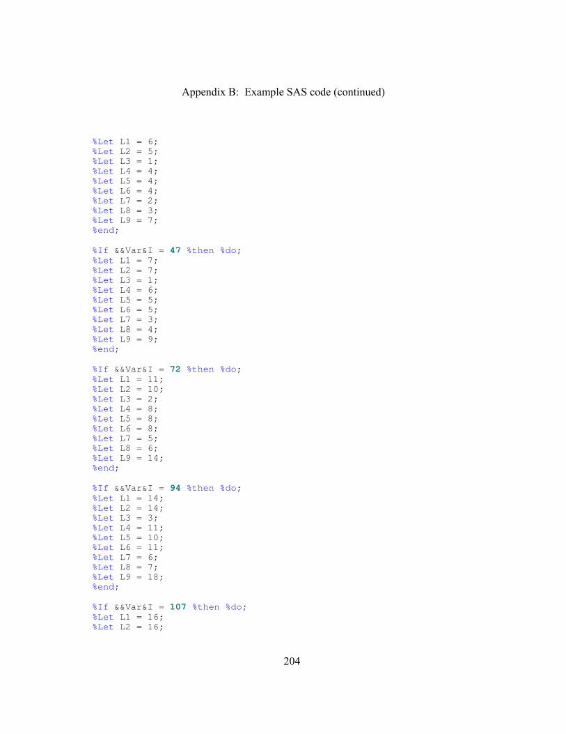
Appendix B: Example SAS code (continued)
204
%Let L1 = 6; %Let L2 = 5; %Let L3 = 1; %Let L4 = 4; %Let L5 = 4; %Let L6 = 4; %Let L7 = 2; %Let L8 = 3; %Let L9 = 7; %end; %If &&Var&I = 47 %then %do; %Let L1 = 7; %Let L2 = 7; %Let L3 = 1; %Let L4 = 6; %Let L5 = 5; %Let L6 = 5; %Let L7 = 3; %Let L8 = 4; %Let L9 = 9; %end; %If &&Var&I = 72 %then %do; %Let L1 = 11; %Let L2 = 10; %Let L3 = 2; %Let L4 = 8; %Let L5 = 8; %Let L6 = 8; %Let L7 = 5; %Let L8 = 6; %Let L9 = 14; %end; %If &&Var&I = 94 %then %do; %Let L1 = 14; %Let L2 = 14; %Let L3 = 3; %Let L4 = 11; %Let L5 = 10; %Let L6 = 11; %Let L7 = 6; %Let L8 = 7; %Let L9 = 18; %end; %If &&Var&I = 107 %then %do; %Let L1 = 16; %Let L2 = 16;
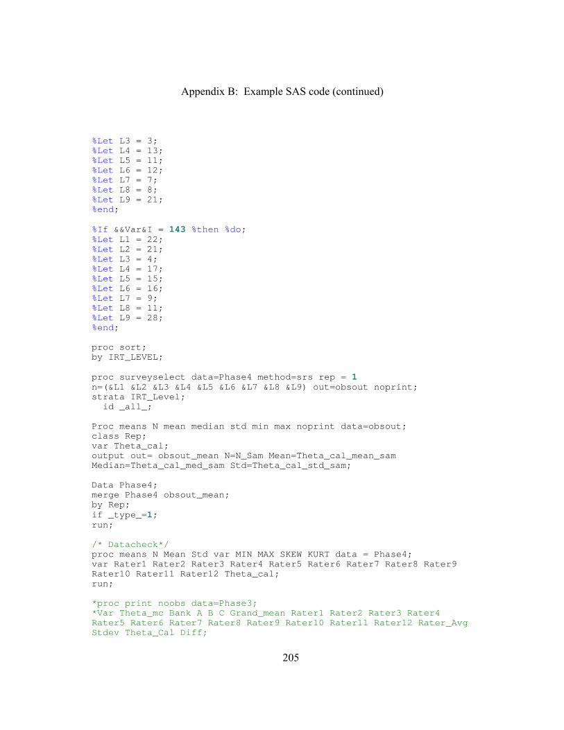
Appendix B: Example SAS code (continued)
205
%Let L3 = 3; %Let L4 = 13; %Let L5 = 11; %Let L6 = 12; %Let L7 = 7; %Let L8 = 8; %Let L9 = 21; %end; %If &&Var&I = 143 %then %do; %Let L1 = 22; %Let L2 = 21; %Let L3 = 4; %Let L4 = 17; %Let L5 = 15; %Let L6 = 16; %Let L7 = 9; %Let L8 = 11; %Let L9 = 28; %end; proc sort; by IRT_LEVEL; proc surveyselect data=Phase4 method=srs rep = 1 n=(&L1 &L2 &L3 &L4 &L5 &L6 &L7 &L8 &L9) out=obsout noprint; strata IRT_Level; id _all_; Proc means N mean median std min max noprint data=obsout; class Rep; var Theta_cal; output out= obsout_mean N=N_Sam Mean=Theta_cal_mean_sam Median=Theta_cal_med_sam Std=Theta_cal_std_sam; Data Phase4; merge Phase4 obsout_mean; by Rep; if _type_=1; run; /* Datacheck*/ proc means N Mean Std var MIN MAX SKEW KURT data = Phase4; var Rater1 Rater2 Rater3 Rater4 Rater5 Rater6 Rater7 Rater8 Rater9 Rater10 Rater11 Rater12 Theta_cal; run; *proc print noobs data=Phase3; *Var Theta_mc Bank A B C Grand_mean Rater1 Rater2 Rater3 Rater4 Rater5 Rater6 Rater7 Rater8 Rater9 Rater10 Rater11 Rater12 Rater_Avg Stdev Theta_Cal Diff;
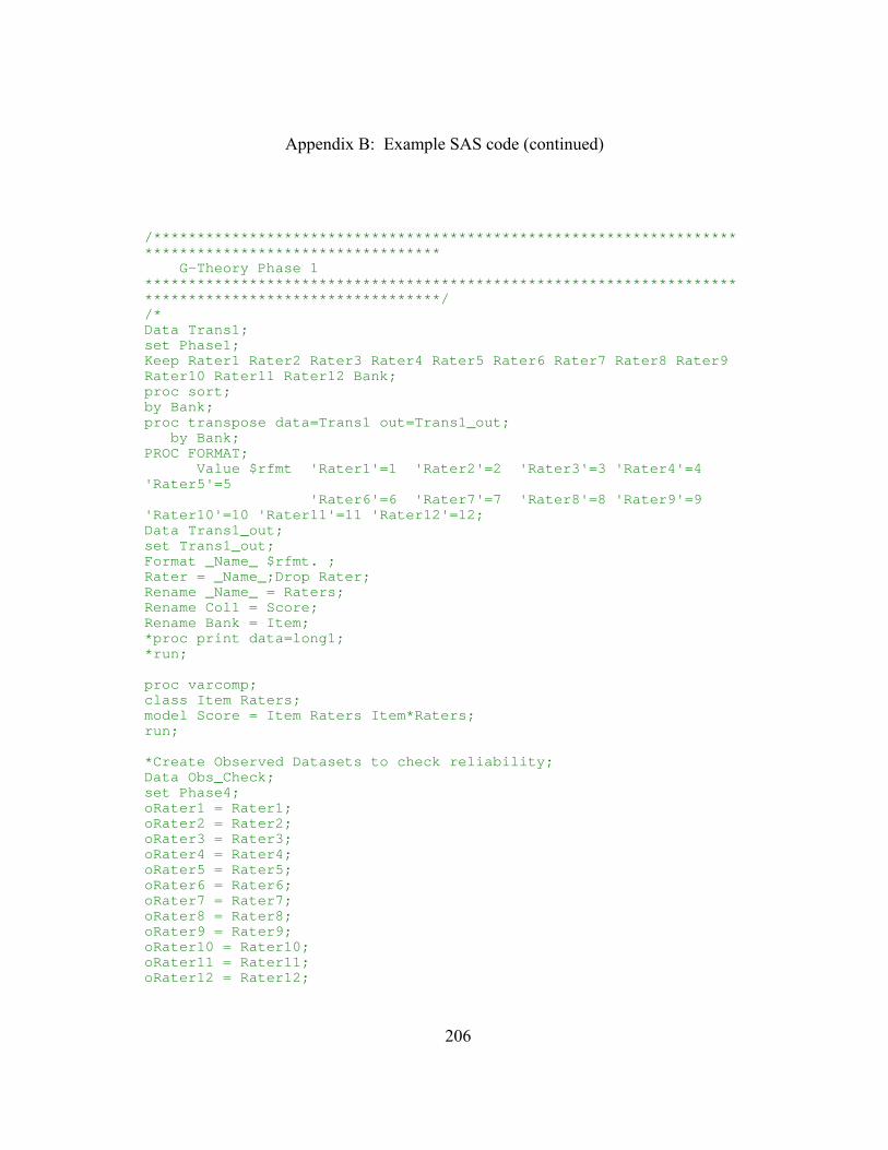
Appendix B: Example SAS code (continued)
206
/***************************************************************************************************** G-Theory Phase 1 ******************************************************************************************************/ /* Data Trans1; set Phase1; Keep Rater1 Rater2 Rater3 Rater4 Rater5 Rater6 Rater7 Rater8 Rater9 Rater10 Rater11 Rater12 Bank; proc sort; by Bank; proc transpose data=Trans1 out=Trans1_out; by Bank; PROC FORMAT; Value $rfmt 'Rater1'=1 'Rater2'=2 'Rater3'=3 'Rater4'=4 'Rater5'=5 'Rater6'=6 'Rater7'=7 'Rater8'=8 'Rater9'=9 'Rater10'=10 'Rater11'=11 'Rater12'=12; Data Trans1_out; set Trans1_out; Format _Name_ $rfmt. ; Rater = _Name_;Drop Rater; Rename _Name_ = Raters; Rename Col1 = Score; Rename Bank = Item; *proc print data=long1; *run; proc varcomp; class Item Raters; model Score = Item Raters Item*Raters; run; *Create Observed Datasets to check reliability; Data Obs_Check; set Phase4; oRater1 = Rater1; oRater2 = Rater2; oRater3 = Rater3; oRater4 = Rater4; oRater5 = Rater5; oRater6 = Rater6; oRater7 = Rater7; oRater8 = Rater8; oRater9 = Rater9; oRater10 = Rater10; oRater11 = Rater11; oRater12 = Rater12;
Appendix B: Example SAS code (continued)
207
Keep oRater1 oRater2 oRater3 oRater4 oRater5 oRater6 oRater7 oRater8 oRater9 oRater10 oRater11 oRater12; /***************************************************************************************************** G-Theory Phase 2 ******************************************************************************************************/ /* Data Trans2; set Phase2; Keep Rater1 Rater2 Rater3 Rater4 Rater5 Rater6 Rater7 Rater8 Rater9 Rater10 Rater11 Rater12 Bank; proc sort; by Bank; proc transpose data=Trans2 out=Trans2_out; by Bank; PROC FORMAT; Value $rfmt 'Rater1'=1 'Rater2'=2 'Rater3'=3 'Rater4'=4 'Rater5'=5 'Rater6'=6 'Rater7'=7 'Rater8'=8 'Rater9'=9 'Rater10'=10 'Rater11'=11 'Rater12'=12; Data Trans2_out; set Trans2_out; Format _Name_ $rfmt. ; Rater = _Name_;Drop Rater; Rename _Name_ = Raters; Rename Col1 = Score; Rename Bank = Item; proc varcomp data=Trans2_out; class Item Raters; model Score = Item Raters Item*Raters; run; /***************************************************************************************************** G-Theory Phase 3 ******************************************************************************************************/ /* Data Trans2; set Phase3; Keep Rater1 Rater2 Rater3 Rater4 Rater5 Rater6 Rater7 Rater8 Rater9 Rater10 Rater11 Rater12 Bank; proc sort; by Bank; proc transpose data=Trans2 out=Trans2_out; by Bank; PROC FORMAT;
Appendix B: Example SAS code (continued)
208
Value $rfmt 'Rater1'=1 'Rater2'=2 'Rater3'=3 'Rater4'=4 'Rater5'=5 'Rater6'=6 'Rater7'=7 'Rater8'=8 'Rater9'=9 'Rater10'=10 'Rater11'=11 'Rater12'=12; Data Trans2_out; set Trans2_out; Format _Name_ $rfmt. ; Rater = _Name_;Drop Rater; Rename _Name_ = Raters; Rename Col1 = Score; Rename Bank = Item; proc varcomp data=Trans2_out; class Item Raters; model Score = Item Raters Item*Raters; run; /***************************************************************************************************** G-Theory Phase 4 ******************************************************************************************************/ /* Data Trans2; set Phase4; Keep Rater1 Rater2 Rater3 Rater4 Rater5 Rater6 Rater7 Rater8 Rater9 Rater10 Rater11 Rater12 Bank; proc sort; by Bank; proc transpose data=Trans2 out=Trans2_out; by Bank; PROC FORMAT; Value $rfmt 'Rater1'=1 'Rater2'=2 'Rater3'=3 'Rater4'=4 'Rater5'=5 'Rater6'=6 'Rater7'=7 'Rater8'=8 'Rater9'=9 'Rater10'=10 'Rater11'=11 'Rater12'=12; Data Trans2_out; set Trans2_out; Format _Name_ $rfmt. ; Rater = _Name_;Drop Rater; Rename _Name_ = Raters; Rename Col1 = Score; Rename Bank = Item; proc varcomp data=Trans2_out; class Item Raters; model Score = Item Raters Item*Raters; run; /*****************************************************************************************************
Appendix B: Example SAS code (continued)
209
START Check Error ******************************************************************************************************/ /* Data rel_check&Rep; set Obs_check; keep oRater1 oRater3 oRater5 oRater6 oRater9 oRater12; Rename oRater1 = oRater1R&Rep; Rename oRater3 = oRater3R&Rep; Rename oRater5 = oRater5R&Rep; Rename oRater6 = oRater6R&Rep; Rename oRater9 = oRater9R&Rep; Rename oRater12 = oRater12R&Rep; Data Rater_Reliability; merge True_Check Obs_Check; proc corr data=Rater_Reliability noprint outp=error_check; *proc print data = Obs; *var r_xx2 Err_SD2 RI_Err rater5 rater6; proc corr data=Rater_Reliability; var oRater1 oRater2 oRater3 oRater5 oRater6 oRater9 oRater12; run; Data error_check2; set error_check; if _TYPE_ = 'CORR'; if _Name_ in ('tRater1', 'tRater2', 'tRater3', 'tRater4', 'tRater5', 'tRater6', 'tRater7', 'tRater8', 'tRater9', 'tRater10', 'tRater11', 'tRater12'); Drop tRater1 tRater2 tRater3 tRater4 tRater5 tRater6 tRater7 tRater8 tRater9 tRater10 tRater11 tRater12 _type_ ; data error_check3; set error_check; True =_n_; array vars[*] oRater1- oRater12; do Obs = 1 to 12; if Obs = True then do; r = vars[Obs]; output; end; end; Drop oRater1- oRater12; proc print data=error_check; run; /* END Check Error *************************************/
Appendix B: Example SAS code (continued)
210
/***************************************************************************************************** Phase Compare ******************************************************************************************************/ /* Get Phase1 Standard */ proc means data = Phase1 noprint; ID Rep Rel Per Direct theta_mc; var Rater_Avg Theta_cal Phase; output out = Phase1_Stand median = Rater_median Theta_median mean = Rater_mean Theta_mean Phase std = Rater_std Theta_std; /* Get Phase2 Standard */ proc means data = Phase2 noprint; ID Rep Rel Per Direct theta_mc; var Rater_Avg Theta_cal Phase; output out = Phase2_Stand median = Rater_median Theta_median mean = Rater_mean Theta_mean Phase std = Rater_std Theta_std; /* Get Phase3 Standard */ proc means data = Phase3 noprint; ID Rep Rel Per Direct theta_mc; var Rater_Avg Theta_cal Phase; output out = Phase3_Stand median = Rater_median Theta_median mean = Rater_mean Theta_mean Phase std = Rater_std Theta_std; /* Get Phase4 Standard */ proc means data = Phase4 noprint; ID Rep Rel Per Direct theta_mc; var Rater_Avg Theta_cal Theta_cal_mean_sam Theta_cal_med_sam Theta_cal_std_sam N_Sam Phase; output out = Phase4_Stand&Rep median = Rater_median Theta_median mean = Rater_mean Theta_mean Theta_cal_mean_sam_mean Theta_cal_med_sam_mean Theta_cal_std_sam_mean N_Sam Phase std = Rater_std Theta_std ; /* Merge data files */ PROC APPEND BASE=Phase1_Stand DATA=Phase2_Stand; PROC APPEND BASE=Phase1_Stand DATA=Phase3_Stand; Data Phase4_lite; Set Phase4_Stand&Rep; DROP Theta_cal_mean_sam_mean Theta_cal_med_sam_mean Theta_cal_std_sam_mean N_Sam;
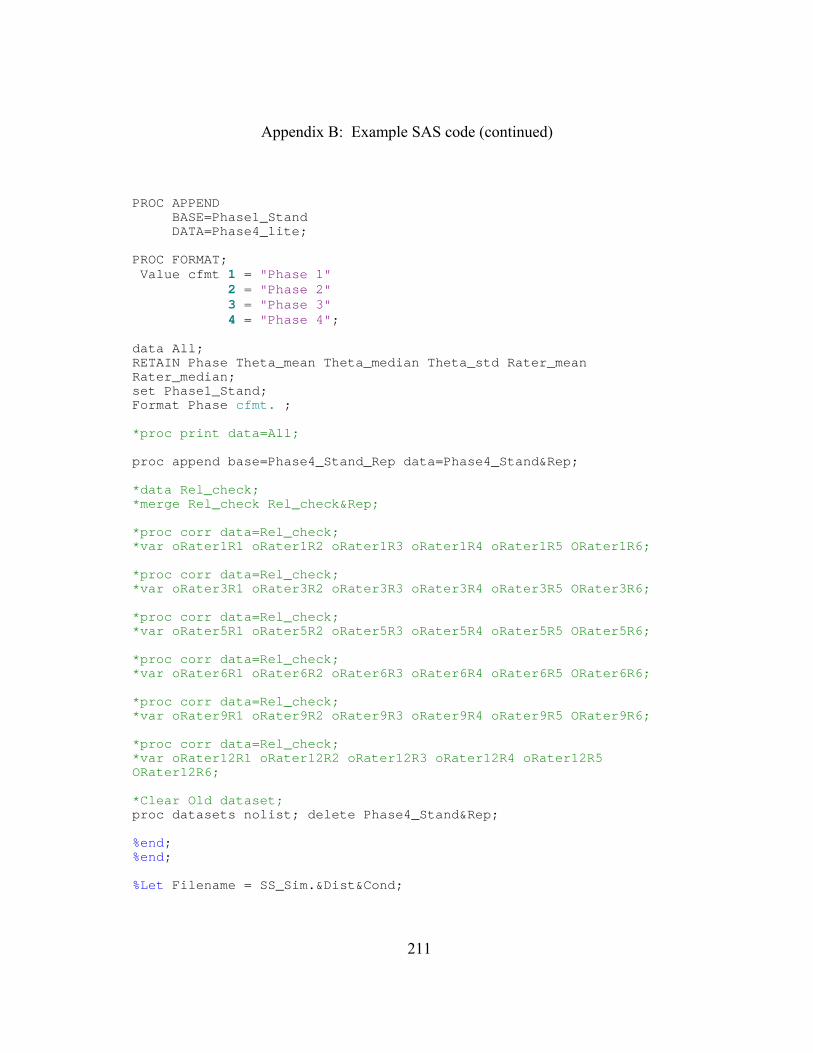
Appendix B: Example SAS code (continued)
211
PROC APPEND BASE=Phase1_Stand DATA=Phase4_lite; PROC FORMAT; Value cfmt 1 = "Phase 1" 2 = "Phase 2" 3 = "Phase 3" 4 = "Phase 4"; data All; RETAIN Phase Theta_mean Theta_median Theta_std Rater_mean Rater_median; set Phase1_Stand; Format Phase cfmt. ; *proc print data=All; proc append base=Phase4_Stand_Rep data=Phase4_Stand&Rep; *data Rel_check; *merge Rel_check Rel_check&Rep; *proc corr data=Rel_check; *var oRater1R1 oRater1R2 oRater1R3 oRater1R4 oRater1R5 ORater1R6; *proc corr data=Rel_check; *var oRater3R1 oRater3R2 oRater3R3 oRater3R4 oRater3R5 ORater3R6; *proc corr data=Rel_check; *var oRater5R1 oRater5R2 oRater5R3 oRater5R4 oRater5R5 ORater5R6; *proc corr data=Rel_check; *var oRater6R1 oRater6R2 oRater6R3 oRater6R4 oRater6R5 ORater6R6; *proc corr data=Rel_check; *var oRater9R1 oRater9R2 oRater9R3 oRater9R4 oRater9R5 ORater9R6; *proc corr data=Rel_check; *var oRater12R1 oRater12R2 oRater12R3 oRater12R4 oRater12R5 ORater12R6; *Clear Old dataset; proc datasets nolist; delete Phase4_Stand&Rep; %end; %end; %Let Filename = SS_Sim.&Dist&Cond;
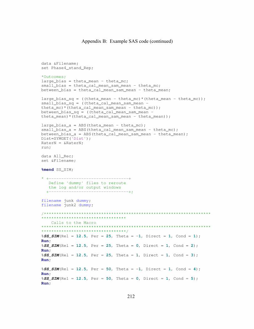
Appendix B: Example SAS code (continued)
212
data &Filename; set Phase4_stand_Rep; *Outcomes; large_bias = theta_mean - theta_mc; small_bias = theta_cal_mean_sam_mean - theta_mc; between_bias = theta_cal_mean_sam_mean - theta_mean; large_bias_sq = ((theta_mean - theta_mc)*(theta_mean - theta_mc)); small_bias_sq = ((theta_cal_mean_sam_mean - theta_mc)*(theta_cal_mean_sam_mean - theta_mc)); between_bias_sq = ((theta_cal_mean_sam_mean - theta_mean)*(theta_cal_mean_sam_mean - theta_mean)); large_bias_a = ABS(theta_mean - theta_mc); small_bias_a = ABS(theta_cal_mean_sam_mean - theta_mc); between_bias_a = ABS(theta_cal_mean_sam_mean - theta_mean); Dist=SYMGET('Dist'); RaterN = &RaterN; run; data All_Rec; set &Filename; %mend SS_SIM; * +--------------------------------+ Define 'dummy' files to reroute the log and/or output windows +--------------------------------+; filename junk dummy; filename junk2 dummy; /***************************************************************************************************** Calls to the Macro ******************************************************************************************************/ %SS_SIM(Rel = 12.5, Per = 25, Theta = -1, Direct = 1, Cond = 1); Run; %SS_SIM(Rel = 12.5, Per = 25, Theta = 0, Direct = 1, Cond = 2); Run; %SS_SIM(Rel = 12.5, Per = 25, Theta = 1, Direct = 1, Cond = 3); Run; %SS_SIM(Rel = 12.5, Per = 50, Theta = -1, Direct = 1, Cond = 4); Run; %SS_SIM(Rel = 12.5, Per = 50, Theta = 0, Direct = 1, Cond = 5); Run;
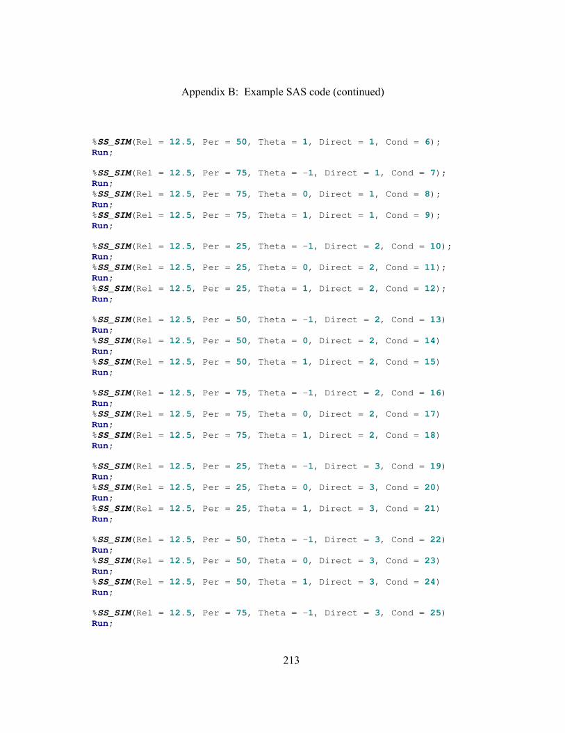
Appendix B: Example SAS code (continued)
213
%SS_SIM(Rel = 12.5, Per = 50, Theta = 1, Direct = 1, Cond = 6); Run; %SS_SIM(Rel = 12.5, Per = 75, Theta = -1, Direct = 1, Cond = 7); Run; %SS_SIM(Rel = 12.5, Per = 75, Theta = 0, Direct = 1, Cond = 8); Run; %SS_SIM(Rel = 12.5, Per = 75, Theta = 1, Direct = 1, Cond = 9); Run; %SS_SIM(Rel = 12.5, Per = 25, Theta = -1, Direct = 2, Cond = 10); Run; %SS_SIM(Rel = 12.5, Per = 25, Theta = 0, Direct = 2, Cond = 11); Run; %SS_SIM(Rel = 12.5, Per = 25, Theta = 1, Direct = 2, Cond = 12); Run; %SS_SIM(Rel = 12.5, Per = 50, Theta = -1, Direct = 2, Cond = 13) Run; %SS_SIM(Rel = 12.5, Per = 50, Theta = 0, Direct = 2, Cond = 14) Run; %SS_SIM(Rel = 12.5, Per = 50, Theta = 1, Direct = 2, Cond = 15) Run; %SS_SIM(Rel = 12.5, Per = 75, Theta = -1, Direct = 2, Cond = 16) Run; %SS_SIM(Rel = 12.5, Per = 75, Theta = 0, Direct = 2, Cond = 17) Run; %SS_SIM(Rel = 12.5, Per = 75, Theta = 1, Direct = 2, Cond = 18) Run; %SS_SIM(Rel = 12.5, Per = 25, Theta = -1, Direct = 3, Cond = 19) Run; %SS_SIM(Rel = 12.5, Per = 25, Theta = 0, Direct = 3, Cond = 20) Run; %SS_SIM(Rel = 12.5, Per = 25, Theta = 1, Direct = 3, Cond = 21) Run; %SS_SIM(Rel = 12.5, Per = 50, Theta = -1, Direct = 3, Cond = 22) Run; %SS_SIM(Rel = 12.5, Per = 50, Theta = 0, Direct = 3, Cond = 23) Run; %SS_SIM(Rel = 12.5, Per = 50, Theta = 1, Direct = 3, Cond = 24) Run; %SS_SIM(Rel = 12.5, Per = 75, Theta = -1, Direct = 3, Cond = 25) Run;
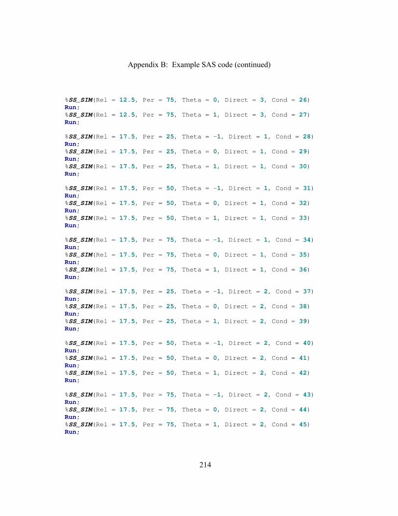
Appendix B: Example SAS code (continued)
214
%SS_SIM(Rel = 12.5, Per = 75, Theta = 0, Direct = 3, Cond = 26) Run; %SS_SIM(Rel = 12.5, Per = 75, Theta = 1, Direct = 3, Cond = 27) Run; %SS_SIM(Rel = 17.5, Per = 25, Theta = -1, Direct = 1, Cond = 28) Run; %SS_SIM(Rel = 17.5, Per = 25, Theta = 0, Direct = 1, Cond = 29) Run; %SS_SIM(Rel = 17.5, Per = 25, Theta = 1, Direct = 1, Cond = 30) Run; %SS_SIM(Rel = 17.5, Per = 50, Theta = -1, Direct = 1, Cond = 31) Run; %SS_SIM(Rel = 17.5, Per = 50, Theta = 0, Direct = 1, Cond = 32) Run; %SS_SIM(Rel = 17.5, Per = 50, Theta = 1, Direct = 1, Cond = 33) Run; %SS_SIM(Rel = 17.5, Per = 75, Theta = -1, Direct = 1, Cond = 34) Run; %SS_SIM(Rel = 17.5, Per = 75, Theta = 0, Direct = 1, Cond = 35) Run; %SS_SIM(Rel = 17.5, Per = 75, Theta = 1, Direct = 1, Cond = 36) Run; %SS_SIM(Rel = 17.5, Per = 25, Theta = -1, Direct = 2, Cond = 37) Run; %SS_SIM(Rel = 17.5, Per = 25, Theta = 0, Direct = 2, Cond = 38) Run; %SS_SIM(Rel = 17.5, Per = 25, Theta = 1, Direct = 2, Cond = 39) Run; %SS_SIM(Rel = 17.5, Per = 50, Theta = -1, Direct = 2, Cond = 40) Run; %SS_SIM(Rel = 17.5, Per = 50, Theta = 0, Direct = 2, Cond = 41) Run; %SS_SIM(Rel = 17.5, Per = 50, Theta = 1, Direct = 2, Cond = 42) Run; %SS_SIM(Rel = 17.5, Per = 75, Theta = -1, Direct = 2, Cond = 43) Run; %SS_SIM(Rel = 17.5, Per = 75, Theta = 0, Direct = 2, Cond = 44) Run; %SS_SIM(Rel = 17.5, Per = 75, Theta = 1, Direct = 2, Cond = 45) Run;
Appendix B: Example SAS code (continued)
215
%SS_SIM(Rel = 17.5, Per = 25, Theta = -1, Direct = 3, Cond = 46) Run; %SS_SIM(Rel = 17.5, Per = 25, Theta = 0, Direct = 3, Cond = 47) Run; %SS_SIM(Rel = 17.5, Per = 25, Theta = 1, Direct = 3, Cond = 48) Run; %SS_SIM(Rel = 17.5, Per = 50, Theta = -1, Direct = 3, Cond = 49) Run; %SS_SIM(Rel = 17.5, Per = 50, Theta = 0, Direct = 3, Cond = 50) Run; %SS_SIM(Rel = 17.5, Per = 50, Theta = 1, Direct = 3, Cond = 51) Run; %SS_SIM(Rel = 17.5, Per = 75, Theta = -1, Direct = 3, Cond = 52) Run; %SS_SIM(Rel = 17.5, Per = 75, Theta = 0, Direct = 3, Cond = 53) Run; %SS_SIM(Rel = 17.5, Per = 75, Theta = 1, Direct = 3, Cond = 54) Run; %SS_SIM(Rel = 21.0, Per = 25, Theta = -1, Direct = 1, Cond = 55) Run; %SS_SIM(Rel = 21.0, Per = 25, Theta = 0, Direct = 1, Cond = 56) Run; %SS_SIM(Rel = 21.0, Per = 25, Theta = 1, Direct = 1, Cond = 57) Run; %SS_SIM(Rel = 21.0, Per = 50, Theta = -1, Direct = 1, Cond = 58) Run; %SS_SIM(Rel = 21.0, Per = 50, Theta = 0, Direct = 1, Cond = 59) Run; %SS_SIM(Rel = 21.0, Per = 50, Theta = 1, Direct = 1, Cond = 60) Run; %SS_SIM(Rel = 21.0, Per = 75, Theta = -1, Direct = 1, Cond = 61) Run; %SS_SIM(Rel = 21.0, Per = 75, Theta = 0, Direct = 1, Cond = 62) Run; %SS_SIM(Rel = 21.0, Per = 75, Theta = 1, Direct = 1, Cond = 63) Run; %SS_SIM(Rel = 21.0, Per = 25, Theta = -1, Direct = 2, Cond = 64) Run; %SS_SIM(Rel = 21.0, Per = 25, Theta = 0, Direct = 2, Cond = 65) Run; %SS_SIM(Rel = 21.0, Per = 25, Theta = 1, Direct = 2, Cond = 66) Run;
Appendix B: Example SAS code (continued)
216
%SS_SIM(Rel = 21.0, Per = 50, Theta = -1, Direct = 2, Cond = 67) Run; %SS_SIM(Rel = 21.0, Per = 50, Theta = 0, Direct = 2, Cond = 68) Run; %SS_SIM(Rel = 21.0, Per = 50, Theta = 1, Direct = 2, Cond = 69) Run; %SS_SIM(Rel = 21.0, Per = 75, Theta = -1, Direct = 2, Cond = 70) Run; %SS_SIM(Rel = 21.0, Per = 75, Theta = 0, Direct = 2, Cond = 71) Run; %SS_SIM(Rel = 21.0, Per = 75, Theta = 1, Direct = 2, Cond = 72) Run; %SS_SIM(Rel = 21.0, Per = 25, Theta = -1, Direct = 3, Cond = 73) Run; %SS_SIM(Rel = 21.0, Per = 25, Theta = 0, Direct = 3, Cond = 74) Run; %SS_SIM(Rel = 21.0, Per = 25, Theta = 1, Direct = 3, Cond = 75) Run; %SS_SIM(Rel = 21.0, Per = 50, Theta = -1, Direct = 3, Cond = 76) Run; %SS_SIM(Rel = 21.0, Per = 50, Theta = 0, Direct = 3, Cond = 77) Run; %SS_SIM(Rel = 21.0, Per = 50, Theta = 1, Direct = 3, Cond = 78) Run; %SS_SIM(Rel = 21.0, Per = 75, Theta = -1, Direct = 3, Cond = 79) Run; %SS_SIM(Rel = 21.0, Per = 75, Theta = 0, Direct = 3, Cond = 80) Run; %SS_SIM(Rel = 21.0, Per = 75, Theta = 1, Direct = 3, Cond = 81) Run; *+--------------------------------+ Turn on the output window again +--------------------------------+; proc printto log = log; run; proc printto print = print; run; Proc means data=All_Rec n sum mean std; class rel per Direct N_Sam theta_mc;
Appendix B: Example SAS code (continued)
217
var theta_mean between_bias large_bias small_bias between_bias_sq large_bias_sq small_bias_sq between_bias_a large_bias_a small_bias_a; run;
About the Author
James Thomas Coraggio received a bachelor’s degree (BA) in Mass
Communications from the University of South Florida in 1994 and a master’s degree
(M.Ed.) in Curriculum and Instruction with an emphasis in measurement and research
from the University of South Florida in 2002. He has directed test development and
psychometric processes for standardized testing companies at Schroeder Measurement
Technologies and Pearson. He has also worked in the area of measurement, evaluation,
and assessment for Eckerd Youth Alternatives and St. Petersburg College. In addition, he
consulted with doctoral students on dissertation research through the Consulting Office
for Research in Education and taught undergraduate measurement courses both in face-
to-face and online formats. His research has been nominated for the Florida Educational
Research Association distinguished paper two times and recognized as Best Paper for the
Florida Association of Institutional Research Conference. He has been listed in Marquis
Who’s Who in the World (2008).