ANZIAM J. 54 (CTAC2012) pp.C699–C719, 2014 C699

A model of workplace safety incorporatingworker interactions and simple interventions

J. Thew1 T. Bopf2 D. G. Mallet3

(Received 22 December 2012; revised 30 November 2013)

Abstract

Although there was substantial research into the occupational healthand safety sector over the past forty years, this generally focused onstatistical analyses of data related to costs and/or fatalities and injuries.There is a lack of mathematical modelling of the interactions betweenworkers and the resulting safety dynamics of the workplace. There isalso little work investigating the potential impact of different safetyintervention programs prior to their implementation. In this article, wepresent a fundamental, differential equation-based model of workplacesafety that treats worker safety habits similarly to an infectious diseasein an epidemic model. Analytical results for the model, derived viaphase plane and stability analysis, are discussed. The model is coupledwith a model of a generic safety strategy aimed at minimising unsafe

http://journal.austms.org.au/ojs/index.php/ANZIAMJ/article/view/6565gives this article, c© Austral. Mathematical Soc. 2014. Published January 2, 2014, aspart of the Proceedings of the 16th Biennial Computational Techniques and ApplicationsConference. issn 1446-8735. (Print two pages per sheet of paper.) Copies of this articlemust not be made otherwise available on the internet; instead link directly to this url forthis article.

Contents C700

work habits, to produce an optimal control problem. The optimalcontrol model is solved using the forward-backward sweep numericalscheme implemented in Matlab.

Contents1 Introduction and background C700

2 Mathematical model C702

3 Computational implementation C705

4 Results C707

5 Discussion C716

References C717

1 Introduction and background

During the 2009–2010 financial year, out of a total workforce of approximately12 million Australians, 5.3% suffered a work-related injury or illness. Thisresulted in a loss of workplace productivity and cost the Australian governmentin workplace compensation payouts an estimated $60.6 billion or 4.8% of thegross domestic product of the nation.

Occupational Health and Safety (ohs) was studied relatively intensely forthe past four decades with an aim to minimise unsafe work practices andassociated costs. Researchers’ interests spanned a multitude of differentapproaches, including observational studies of existing programs [2, 3, 11],developing new approaches to safety improvement, analysis of governmentalreforms at both national and state levels [4, 5, 10] and analysis of data

1 Introduction and background C701

regarding ohs costs [6, 7, 8]. However, to the authors’ knowledge, therewas no attempt to mathematically model interactions between workers andthe resulting impact on safety dynamics and costs in the workplace. Theapparent shortage of mathematical models presents an opportunity to developa selection of tools to produce a deeper understanding of the effects of differentapproaches in minimising ohs costs. Here we present a preliminary model forthe dynamics of interacting populations of workers who are classified as either‘safe’ or ‘unsafe’. The model is proposed as a basis for further investigationregarding occupational health and safety.

The safety habits observed in a workplace depend greatly upon the regulationand maintenance of safety structures provided by management and govern-ment legislation. Without regulation, there is potential for unsafe practices tobecome more common, increasing the risk of injury or illness in the workplace.This results in decreased productivity through a loss of personnel as well asthe financial costs associated with sick leave, investigating the incident andtraining replacement staff. Independently as well as due to government legis-lation, businesses and industries employ intervention strategies to minimiseworkplace safety incidents and maximise safety. These methods include ohslegislation [21], on-site health and safety officers [20] and the incorporationof risk management into the agenda of the company [9]. While all of theseinterventions are in themselves costly, the objective of the company is to seekgreater benefit by reducing incident related costs by more than the cost ofthe intervention itself. An obvious but important pursuit in business practiceis to limit the cost of running the company, so mathematical models thatare able to describe workplace safety dynamics and investigate the impact ofsafety programs, a priori, are of great value to industry.

We consider the workforce to be split into four groups: safe and unsafe workerswho are currently either on some sort of sick leave or are actively working. Theworkers interact as part of their daily work activities and are able to alter eachothers’ behaviour, resulting in movement between the different populations.The dynamics are modeled using ordinary differential equations (odes) similarto those employed in infectious disease models [13, 16, e.g.]. To incorporate

2 Mathematical model C702

safety interventions and to attempt to investigate cost minimisation, weextend the ode model to an optimal control model.

2 Mathematical model

We explore the dynamics of the workforce, in terms of safety classifications,using a modelling strategy that is similar to the sir models of infectiousdisease modelling [13, 16]. Such models were used successfully to model manydiseases including the plague [13, 17] and measles [19], and modified to modelsexually transmitted diseases such as chlamydia [15]. sir models seek todescribe the spread of an infection in a population over time by trackingthe populations of susceptible (S), infected (I) and recovered (R) individuals.Infected individuals transmit the infection to the susceptibles through somesort of contact, which is modeled as being proportional to the product of thetwo populations. Further details on sir models are found in many sources,but Murray provides an excellent background [16].

The link that we make between sir models of infectious diseases and thestrategy used here to describe worker safety, is to propose that safe behaviourand unsafe behaviour is transmitted in a similar way to the infection in aninfectious disease model. That is, safeness is transmitted to unsafe workers ata rate proportional to the product of the safe and unsafe populations. Unsafebehaviour is transmitted in a similar way.

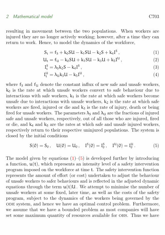
The model involves a system of four odes (1)–(4) where S(t) and U(t)represent the numbers of workers at time t who undertake their jobs in amostly safe manner (‘safe workers’) and unsafe manner (‘unsafe workers’),respectively. Similarly, IS(t) and IU(t) denote the numbers of injured workerswho undertake their jobs in a safe or unsafe way, respectively. We assumethat new workers are constantly entering the workforce, while workers arefired, injured and die at some rate. Safe and unsafe workers interact, passingon behavioral characteristics related to the safety of their work practices,

2 Mathematical model C703

resulting in movement between the two populations. When workers areinjured they are no longer actively working; however, after a time they canreturn to work. Hence, to model the dynamics of the workforce,

St = fS + k0SU− k1SU− k2S+ k4IS , (1)

Ut = fU − k0SU+ k1SU− k3U+ k5IU , (2)

ISt = λSk2S− k4IS , (3)

IUt = λUk3U− k5IU , (4)

where fS and fU denote the constant influx of new safe and unsafe workers,k0 is the rate at which unsafe workers convert to safe behaviour due tointeractions with safe workers, k1 is the rate at which safe workers becomeunsafe due to interactions with unsafe workers, k2 is the rate at which safeworkers are fired, injured or die and k3 is the rate of injury, death or beingfired for unsafe workers. The parameters λS and λU are the fractions of injuredsafe and unsafe workers, respectively, out of all those who are injured, firedor die, and k4 and k5 are the rates at which safe and unsafe injured workers,respectively return to their respective uninjured populations. The system isclosed by the initial conditions

S(0) = S0 , U(0) = U0 , IS(0) = IS0 , IU(0) = IU0 . (5)

The model given by equations (1)–(5) is developed further by introducinga function, u(t), which represents an intensity level of a safety interventionprogram imposed on the workforce at time t. The safety intervention functionrepresents the amount of effort (or cost) undertaken to adjust the behaviourof unsafe workers to safer behaviours and is reflected in the adjusted dynamicequations through the term u(t)U . We attempt to minimise the number ofunsafe workers at some fixed, later time, as well as the costs of the safetyprogram, subject to the dynamics of the workers being governed by theode system, and hence we have an optimal control problem. Furthermore,we assume that we have a bounded problem as most companies will haveset some maximum quantity of resources available for ohs. Thus we have

2 Mathematical model C704

0 6 u(t) 6 umax , where umax is the maximum amount of resources availablefor improving safety. The optimal control problem to be solved is

minu

∫ tend

0

u2(t) dt+U(tend) , 0 6 u(t) 6 umax , (6)

where tend is the fixed end time for the problem, and subject to equations

St = fS + k0SU− k1SU− k2S+ k4IS + u(t)U , (7)

Ut = fU − k0SU+ k1SU− k3U+ k5IU − u(t)U , (8)

ISt = λSk2S− k4IS , (9)

IUt = λUk3U− k5IU , (10)

with initial conditions (5) and free final conditions for all variables.

To solve the optimal control problem, we form the Hamiltonian H and theLagrangian L:

H(t, x,u,σ) = u2 + σ1St + σ2Ut + σ3ISt + σ4IUt , (11)

L(t, x,u,σ) = H(t, x,u,σ) +ω1(t)u(t) +ω2(t)[umax − u(t)], (12)

where σ1, . . . ,σ4 are the adjoint functions, and where the two penalty multi-pliers ω1(t) and ω2(t) satisfy

ω1(t),ω2(t) > 0 , (13)ω1(t),ω2(t) = 0 for 0 < u∗(t) < umax , (14)

ω1(t) = 0 , ω2(t) > 0 for u(t) = 0 , (15)ω2(t) = 0 , ω1(t) > 0 for u(t) = umax . (16)

The concavity condition on the Hamiltonian produces Huu = 2 > 0 , andhence any optimal control will produce a minimum for (6), as required. The

3 Computational implementation C705

adjoint equations are then

−∂H

∂S= σ ′1(t) = − σ1(t)[(k0 − k1)U(t) − k2]

− σ2(t)(k1 − k0)U(t) − σ3(t)λSk2 , (17)

−∂H

∂U= σ ′2(t) = − σ1(t)[(k0 − k1)S(t) + u(t)] − σ4(t)λUk3

− σ2(t)[(k1 − k0)S(t) − k3 − u(t)] , (18)

−∂H

∂IS= σ ′3(t) = k4[σ3(t) − σ1(t)] , (19)

−∂H

∂IU= σ ′4(t) = k5[σ4(t) − σ2(t)] . (20)

Equations (17)–(20) are subject to the tranversality conditions

σ1(tend) = 0 , σ2(tend) = 1 , σ3(tend) = 0 , σ4(tend) = 0 . (21)

The optimality condition is

∂L

∂u

∣∣∣∣u∗(t)

= 2u∗(t) + [σ1(t) − σ2(t)]U(t) +w1(t) −w2(t) = 0 .

Using the optimality condition, along with equations (13)–(16) we obtain theoptimal control

u∗(t) = min[umax, max

(U(t)[µ2(t) − µ1(t)]

2, 0)]

. (22)

When u = u∗ , the system is optimised in the sense of equation (6).

3 Computational implementation

Here we present the algorithm (the forward-backward sweep method) used tosolve the bounded optimal control problem of Section 2. We adapt the single

3 Computational implementation C706

equation scheme outlined by Lenhart [14] to solve the multispecies modelproposed here.

Consider the optimal control problem over time interval [t0, t1] ,

maxu

∫ t1t0

f[t, x(t),u(t)]dt subject to x ′ = g[t, x(t),u(t)] , x(t0) = x0 ,

where x ∈ Rn are the state variables, g is the vector of the right hand sides ofthe state differential equations, u ∈ Rm , n is the number of state equationsand m is the number of controls to be implemented on the system.

Introduce matrices X ∈ Rn×(N+1) , Λ ∈ Rn×(N+1) and U ∈ Rm×(N+1) , whereN+ 1 is the number of time steps to be taken, X is the approximation to xat the N + 1 time steps, and Λ is a matrix of the adjoint equations, suchas (17)–(20). Then the following steps solve the optimal control problem.

1. Make an initial guess U for u in a given time interval.

2. Using the initial condition X(1 : n, 1) = x(t0) and U, solve X forwardin time according to its differential equation in the optimality system.

3. Using the transversality condition, such as equation (21), Λ(1 : n,N+1) = σ(t1) = 0 (where σ are the adjoint functions) and the valuesfor u and X, solve Λ backward in time according to its differentialequation, σ, in the optimality system.

4. Update u and output the current values as solutions. If values are notsufficiently close, then return to step 3 using the updated X and Λvalues.

5. Check convergence. If values of the control variables in this iterationand the last iteration are negligibly close, then control is optimal.

Computationally, the problem is not expensive to solve. We use standard Mat-lab ode solvers to compute results and these are returned usually in 1–2 min-utes using an iMac with 3.1GHz Intel Core i5, 4Gb 1333MHz DDR3 memoryand Matlab 2012a.

4 Results C707

Table 1: Parameter values used in the solution of the optimal control modelobtained from the Australian Bureau of Statistics [1], Safe Work Australia [18]and via calculation and estimation (see main text).

parameter value sourceworkforce 10658000 workers [1]fatalities 254 workers per year [18]injuries 153562.5 workers per year [18]fired 600000 workers per year [18]k2 + k3 0.06626 per year Calc.k4 + k5 0.72 per year Calc.fS + fU 364020 workers per year Calc.λS + λU 0.20371 Calc.

4 Results

In this section, the optimal control problem set up in Section 2 is solved usingthe forward-backward sweep method as discussed in Section 3. First, theparameters of the model are specified in Table 1. Most of the parametersused are drawn from Safe Work Australia reports [18] and the AustralianBureau of Statistics [1].

The parameters that are not taken from the literature are obtained as follows.The rate of workers leaving the workforce is calculated using

k2 + k3 =(fatalities+ injuries+ fired)

workforce.

To accommodate the returning to work parameters of the model, k4 and k5 ,the durable return to work rate is used [12]. The return to work rate states thatan average of 72% of workers returned to work for more than seven monthsafter lodging their claim. As a first approximation we take the recruitmentparameters, fS and fU , to be the difference in the number of workers leavingthe workforce and the number of workers returning to the workforce. The

4 Results C708

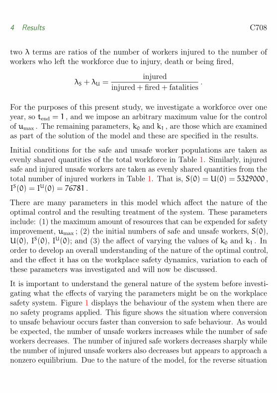
two λ terms are ratios of the number of workers injured to the number ofworkers who left the workforce due to injury, death or being fired,

λS + λU =injured

injured+ fired+ fatalities.

For the purposes of this present study, we investigate a workforce over oneyear, so tend = 1 , and we impose an arbitrary maximum value for the controlof umax . The remaining parameters, k0 and k1 , are those which are examinedas part of the solution of the model and these are specified in the results.

Initial conditions for the safe and unsafe worker populations are taken asevenly shared quantities of the total workforce in Table 1. Similarly, injuredsafe and injured unsafe workers are taken as evenly shared quantities from thetotal number of injured workers in Table 1. That is, S(0) = U(0) = 5329000 ,IS(0) = IU(0) = 76781 .

There are many parameters in this model which affect the nature of theoptimal control and the resulting treatment of the system. These parametersinclude: (1) the maximum amount of resources that can be expended for safetyimprovement, umax ; (2) the initial numbers of safe and unsafe workers, S(0),U(0), IS(0), IU(0); and (3) the affect of varying the values of k0 and k1 . Inorder to develop an overall understanding of the nature of the optimal control,and the effect it has on the workplace safety dynamics, variation to each ofthese parameters was investigated and will now be discussed.

It is important to understand the general nature of the system before investi-gating what the effects of varying the parameters might be on the workplacesafety system. Figure 1 displays the behaviour of the system when there areno safety programs applied. This figure shows the situation where conversionto unsafe behaviour occurs faster than conversion to safe behaviour. As wouldbe expected, the number of unsafe workers increases while the number of safeworkers decreases. The number of injured safe workers decreases sharply whilethe number of injured unsafe workers also decreases but appears to approach anonzero equilibrium. Due to the nature of the model, for the reverse situation

4 Results C709

0 0.2 0.4 0.6 0.8 1

4.5

5

5.5

6

6.5

Time (years)

Uninjured

workersS,U

7.05

7.1

7.15

7.2·10−2

InjuredworkersIS,IU

Figure 1: Solution curves (106 workers) with no safety interventions. Shownare S(t) (thick, solid), U(t) (thick, dash), IS(t) (solid), and IU(t) (dash) forstronger conversion to unsafe behaviour (k1 − k0 = 0.2).

where conversion to safe behaviour is faster, the exact opposite situationis observed with safe and unsafe populations switching curves (result notshown).

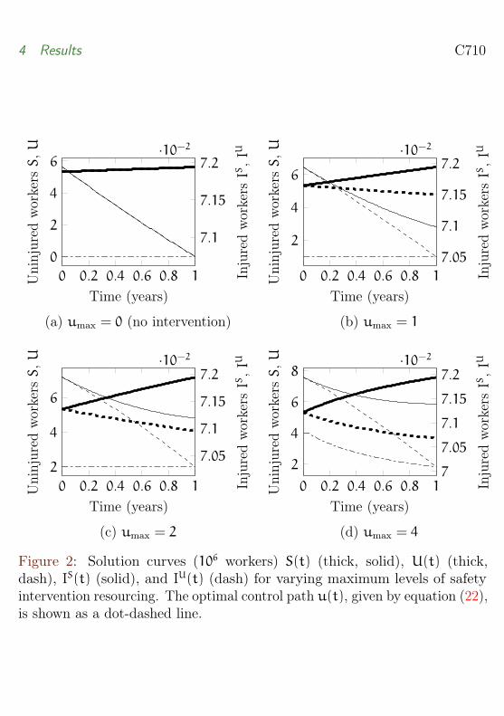
Now we introduce the safety intervention via the optimal control problem andconsider the effect of increasing the amount of resources available to implementthe safety program. Figure 2 shows that as the amount of resourcing appliedto safety interventions increases, solution behaviour changes markedly. Inparticular, we note (pleasingly) that the unsafe worker population decreaseswhile the safe worker population increases, with both approaching whatappears to be steady levels. Increasing the maximum amount of controlbeyond that shown in Figure 2 results in a surplus that is not utilised.Solutions quantitatively reproduce those shown in Figure 2.

4 Results C710

0 0.2 0.4 0.6 0.8 1

0

2

4

6

Time (years)

Uninjured

workersS,U

7.1

7.15

7.2·10−2

InjuredworkersIS,IU

(a) umax = 0 (no intervention)

0 0.2 0.4 0.6 0.8 1

2

4

6

Time (years)Uninjured

workersS,U

7.05

7.1

7.15

7.2·10−2

InjuredworkersIS,IU

(b) umax = 1

0 0.2 0.4 0.6 0.8 1

2

4

6

Time (years)

Uninjured

workersS,U

7.05

7.1

7.15

7.2·10−2

InjuredworkersIS,IU

(c) umax = 2

0 0.2 0.4 0.6 0.8 1

2

4

6

8

Time (years)

Uninjured

workersS,U

7

7.05

7.1

7.15

7.2·10−2

InjuredworkersIS,IU

(d) umax = 4

Figure 2: Solution curves (106 workers) S(t) (thick, solid), U(t) (thick,dash), IS(t) (solid), and IU(t) (dash) for varying maximum levels of safetyintervention resourcing. The optimal control path u(t), given by equation (22),is shown as a dot-dashed line.

4 Results C711

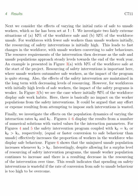
Next we consider the effects of varying the initial ratio of safe to unsafeworkers, which so far has been set at 1 : 1. We investigate two fairly extremesituations of (a) 10% of the workforce safe and (b) 10% of the workforceunsafe. For workforces with fewer safe workers than unsafe workers initially,the resourcing of safety interventions is initially high. This leads to fastchanges in the workforce, with unsafe workers converting to safer behaviours.The resource requirements of the intervention then decrease as the safe andunsafe populations approach steady levels towards the end of the work year.An example is presented in Figure 3(a) with 10% of the workforce safe atthe start of the project. Resourcing of safety interventions is important here,where unsafe workers outnumber safe workers, as the impact of the programis quite strong. Also, the effects of the safety intervention are maintained inthe long term with decreasing levels of resourcing. However, for workforceswith initially high levels of safe workers, the impact of the safety programs isweaker. In Figure 3(b) we see the case where initially 90% of the workforcedisplay safe work habits. Here, there is basically no impact on the workerpopulations from the safety interventions. It could be argued that any effortor expense resulting from attempting to impose such interventions is wasted.

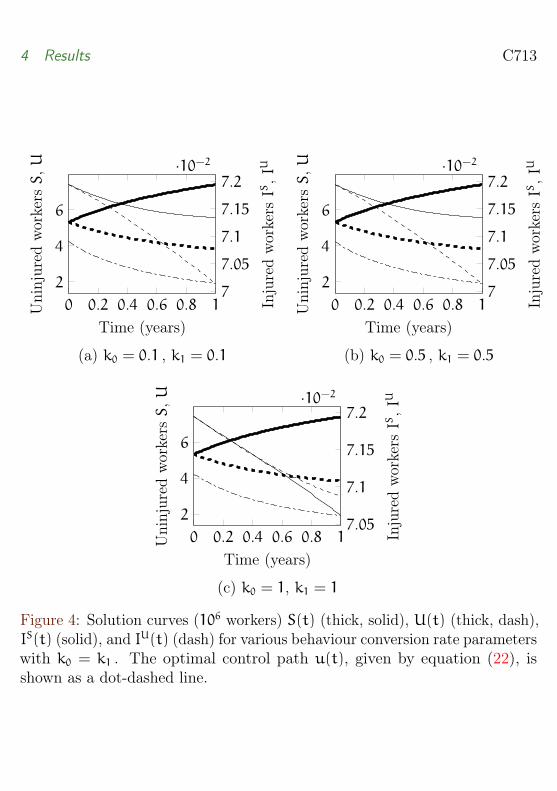
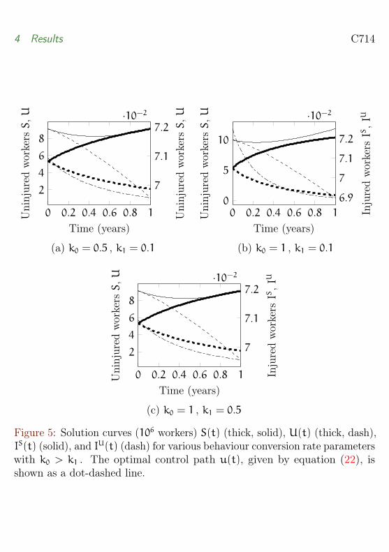
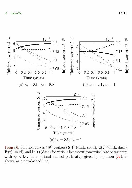
Finally, we investigate the effects on the population dynamics of varying theinteraction rates k0 and k1 . Figures 4–6 display the results from a numberof numerical solutions with varied values for the interaction parameters. ForFigures 4 and 5 the safety intervention program coupled with k0 = k1 ork0 > k1, respectively, (equal or faster conversion to safe behaviour thanunsafe) effectively increases the proportion of workers in the workforce whodisplay safe behaviour. Figure 6 shows that the uninjured unsafe populationincreases whenever k1 > k0 . Interestingly, despite allowing for a surplus levelof resourcing of safety intervention programs, the unsafe worker populationcontinues to increase and there is a resulting decrease in the resourcingof the intervention over time. This result indicates that spending on safetyinterventions is wasteful if the rate of conversion from safe to unsafe behaviouris too high to be overcome.

4 Results C712

0 0.2 0.4 0.6 0.8 1

2

4

6

8

10

Time (years)

Uninjured

workersS,U

5

10

·10−2

InjuredworkersIS,IU

(a) 10% safe workers

0 0.2 0.4 0.6 0.8 1

0

5

10

Time (years)

Uninjured

workersS,U

5

10

15·10−2

InjuredworkersIS,IU

(b) 90% safe workers

Figure 3: Solution curves (106 workers) S(t) (thick, solid), U(t) (thick, dash),IS(t) (solid), and IU(t) (dash) for varying initial ratios of safe : unsafe workers.The optimal control path u(t), given by equation (22), is shown as a dot-dashed line.

4 Results C713

0 0.2 0.4 0.6 0.8 1

2

4

6

Time (years)

Uninjured

workersS,U

7

7.05

7.1

7.15

7.2·10−2

InjuredworkersIS,IU

(a) k0 = 0.1 , k1 = 0.1

0 0.2 0.4 0.6 0.8 1

2

4

6

Time (years)Uninjured

workersS,U

7

7.05

7.1

7.15

7.2·10−2

InjuredworkersIS,IU

(b) k0 = 0.5 , k1 = 0.5

0 0.2 0.4 0.6 0.8 1

2

4

6

Time (years)

Uninjured

workersS,U

7.05

7.1

7.15

7.2·10−2

InjuredworkersIS,IU

(c) k0 = 1, k1 = 1

Figure 4: Solution curves (106 workers) S(t) (thick, solid), U(t) (thick, dash),IS(t) (solid), and IU(t) (dash) for various behaviour conversion rate parameterswith k0 = k1 . The optimal control path u(t), given by equation (22), isshown as a dot-dashed line.

4 Results C714

0 0.2 0.4 0.6 0.8 1

2

4

6

8

Time (years)

Uninjured

workersS,U

7

7.1

7.2·10−2

Uninjured

workersS,U

(a) k0 = 0.5 , k1 = 0.1

0 0.2 0.4 0.6 0.8 10

5

10

Time (years)

Uninjured

workersS,U

6.9

7

7.1

7.2

·10−2

InjuredworkersIS,IU

(b) k0 = 1 , k1 = 0.1

0 0.2 0.4 0.6 0.8 1

2

4

6

8

Time (years)

Uninjured

workersS,U

7

7.1

7.2·10−2

InjuredworkersIS,IU

(c) k0 = 1 , k1 = 0.5

Figure 5: Solution curves (106 workers) S(t) (thick, solid), U(t) (thick, dash),IS(t) (solid), and IU(t) (dash) for various behaviour conversion rate parameterswith k0 > k1 . The optimal control path u(t), given by equation (22), isshown as a dot-dashed line.

4 Results C715

0 0.2 0.4 0.6 0.8 1

3

4

5

6

Time (years)

Uninjured

workersS,U

7.05

7.1

7.15

7.2·10−2

InjuredworkersIS,IU

(a) k0 = 0.1 , k1 = 0.5

0 0.2 0.4 0.6 0.8 13

4

5

6

Time (years)Uninjured

workersS,U

7.05

7.1

7.15

7.2·10−2

InjuredworkersIS,IU

(b) k0 = 0.1 , k1 = 1

0 0.2 0.4 0.6 0.8 1

3

4

5

6

Time (years)

Uninjured

workersS,U

7.05

7.1

7.15

7.2·10−2

InjuredworkersIS,IU

(c) k0 = 0.5 , k1 = 1

Figure 6: Solution curves (106 workers) S(t) (thick, solid), U(t) (thick, dash),IS(t) (solid), and IU(t) (dash) for various behaviour conversion rate parameterswith k0 < k1 . The optimal control path u(t), given by equation (22), isshown as a dot-dashed line.

5 Discussion C716

5 Discussion

We presented a prototype model of the dynamics of populations of workers,classified according to their safety behaviour. The model draws on infectiousdisease modelling and treats safe and unsafe behaviour similarly to a diseasethat can be ‘caught’ from another worker who already displays that behaviour.We also incorporated simple safety intervention programs theoretically via anoptimal control problem that seeks to minimise unsafe workers and the costsdue to the safety interventions. This model was solved using a multispeciesimplementation of the forward-backward sweep method for solving optimallycontrolled systems of odes.

Our results focus on investigating the effects of varying the level of resourcingavailable to safety interventions, the initial ratio of safe to unsafe workers inthe workforce, and the safe and unsafe behavioural transmission rates. Wefound that increasing the amount of resourcing to provide safety interventionsis effective in reducing the unsafe worker population toward a stable levelthat is maintained with reduced levels of resourcing. We also found thatfor workforces with initially high proportions of safe workers, the impact ofsafety interventions is quite limited and perhaps not worth the cost of settingup such programs. This could be quite an important finding for industriesthat are known to have very few unsafe workers. Finally, the investigation ofthe rates of conversion between safe and unsafe practices indicated that forworkforces where the conversion to unsafe behaviour is very high, the safetyinterventions have little effect on the increasing unsafe worker populations. Assuch, again, the costs of imposing the type of simple interventions investigatedhere perhaps outweigh any benefits observed.

A goal of the ohs sector is to reduce the number of safety-related workplaceincidents so it is not surprising that substantial effort is directed towardsfinding the most at-risk industries. In Australia, two such industries are theconstruction industry and agricultural/logging industries [18]. Additionally,inexperienced workers are also classified as an at risk group for ohs. Future

References C717

research will adapt the modelling work carried out here to investigate suchspecific industries and worker cohorts.

References

[1] Australian Bureau of Statistics. Forms of employment. Commonwealthof Australia, 2010. http://www.abs.gov.au/AUSSTATS/abs@.nsf/DetailsPage/6359.0November%202010?OpenDocument C707

[2] Bahn, S. Power and Influence: Examining the Communication Pathwaysthat Impact on Safety in the Workplace. J. Occup. Health Safety—Aust.N.Z., 25(3):213–222, 2009. C700

[3] Bird, P. Reducing Manual Handling Workers Compensation Claims in aPublic Health Facility. J. Occup. Health Safety—Aust. N.Z.,25(6):451–459, 2009. C700

[4] Breslin, P. Improving ohs Standards in the Building and ConstructionIndustry through safe design. J. Occup. Health Safety—Aust. N.Z.,23(4):89–99, 2007. C700

[5] Breslin, P. National Harmonisation: Designers’ Duties of Care in theAustralian Building and Construction Industry. J. Occup. HealthSafety—Aust. N.Z., 25(6):495–504, 2009 . C700

[6] Driscoll, T., Mitchell, T., Mandryk, J., Healey, S., Hendrie, L. and Hull,B. Trends in Work-Related Fatalities in Australia, 1982 to 1992. J.Occup. Health Safety—Aust. N.Z., 18(1):21–33, 2002. C701

[7] Driscoll, T. Fatal Injury of young workers in Australia. J. Occup.Health Safety—Aust. N.Z., 22(2):151–161, 2006. C701

[8] Foley, G., Gale, J. and Gavenlock, L. The Cost of Work-Related Injuryand Disease. J. Occup. Health Safety—Aust. N.Z., 11(2):171–194, 1995.C701

References C718

[9] Glendon, I. and Waring, A. Risk management as a framework foroccupational health and safety. J. Occup. Health Safety—Aust. N.Z.,13(6):525–532, 1997. C701

[10] Gunningham, N. and Healy, P. Agricultural ohs Policy: TowardsSystemic Reform. J. Occup. Health Safety—Aust. N.Z., 20(4):311–318,2004. C700

[11] Hawkins, A., Eather, J. and Fragar, L. Improving Health and Safety inthe Farm Workshop. J. Occup. Health Safety—Aust. N.Z.,24(2):155–160, 2008. C700

[12] Heads of Workers’ Compensation Authorities. 2008/09 Australia andNew Zealand Return to Work Monitor.http://www.hwca.org.au/documents/Australia%20and%20New%20Zealand%20Return%20to%20Work%20Monitor%202008-2009.pdfC707

[13] Kermack, W. O. and McKendrick, A. G. A Contribution to theMathematical Theory of Epidemics. Proc. R. Soc. Lond. A.,115(772):700–721, 1927. doi:10.1098/rspa.1927.0118 C701, C702

[14] Lenhart, S. and Workman, J. T. Optimal control applied to biologicalmodels. Chapman & Hall CRC Mathematical and ComputationalBiology Series, 2007. C706

[15] Mallet, D. G., Bagher-Oskouei, M., Farr, A. C., Simpson, D. P. andSutton, K-J. A mathematical model of Chlamydial infectionincorporating movement of Chlamydial particles. B. Math. Biol.,75(11):2257–2270, 2013. doi:10.1007/s11538-013-9891-9 C702

[16] Murray, J. D. Mathematical Biology, I: An Introduction. Springer, 2002.C701, C702

[17] Raggett, G. F. Modelling the Eyam plague. B. I. Math. Appl.,18:221–226, 1982. C702

References C719

[18] Safe Work Australia. The cost of work-related injury and illness foraustralian employers, workers and the community:2008-2009.Commonwealth of Australia, 2012. http://www.safeworkaustralia.gov.au/sites/SWA/about/Publications/Documents/660/Cost%20of%20Work-related%20injury%20and%20disease.pdf C707, C716

[19] Shulgin, B., Stone, L. and Agur, Z. Pulse vaccination strategy in the sirEpidemic Model. B. Math. Biol., 60(6):1123–1148, 1998.doi:10.1006/S0092-8240(98)90005-2 C702

[20] Vanderkruk, R. Workplace health and safety officers: a Queenslandsuccess story. J. Occup. Health Safety—Aust. N.Z., 15(6):557–563, 1999.C701

[21] Winder, C. The development of ohs legislation in Australia. J. Occup.Health Safety—Aust. N.Z., 25(4):277–287, 2009. C701

Author addresses

1. J. Thew, Mathematical Sciences School, Queensland University ofTechnology, Queensland 4000, Australia.

2. T. Bopf, Mathematical Sciences School, Queensland University ofTechnology, Queensland 4000, Australia.

3. D. G. Mallet, Mathematical Sciences School, Queensland Universityof Technology, Queensland 4000, Australia.mailto:dg.mallet@qut.edu.au