A Model of Dynamic Compensation and Capital Structure

Zhiguo He�

April 2010

Abstract

This paper studies the optimal compensation problem between shareholders and the agent

in the Leland (1994) capital structure model, and �nds that the debt-overhang effect on the en-

dogenous managerial incentives lowers the optimal leverage. Consistent with data, our model

delivers a negative relation between pay-performance sensitivity and �rm size, and the interac-

tion between debt-overhang and agency issue leads smaller �rms to take less leverage relative

to their larger peers. During �nancial distress, a �rm's cash-�ow becomes more sensitive to

underlying performance shocks due to debt-overhang. The implications on credit spreads and

debt covenants are also considered.

Key Words: Continuous-time Contracting, Capital Structure, CARA (Exponential) Pref-

erence, Firm Growth, Size-Heterogeneity, Pay-Performance Sensitivity.

�University of Chicago, Booth School of Business, zhiguo.he@chicagobooth.edu. An earlier version of this paperwas circulated under the title �Agency Problems, Firm Valuation, and Capital Structure.� I thank an anonymous referee,Mike Fishman, Arvind Krishnamurthy, Patrick Bolton, Chris Hennessy, Debbie Lucas, Ilya Strabeleuv, and YuriTserlukevich (AFA 2009 discussant) for valuable suggestions. All errors are mine.

1 Introduction

This paper embeds optimal contracting between the agent (manager) and shareholders into the

cash-�ow framework commonly used in the literature of structural models of capital structure

(Leland (1994)). By connecting these two literatures, we provide a general framework to study the

impacts of agency characteristics on �rm valuation and capital structure. Moreover, the dynamic

nature of this framework allows us to calibrate our model, and in turn quantitatively assess the

agency impact on the �rm's leverage decision.

We characterize the optimal contract between shareholders and the agent explicitly. In deter-

mining the leverage level, debt bears an additional �debt-overhang� cost relative to the bankruptcy

cost in standard models (a la Leland (1994)): by interpreting the agent's effort as a form of invest-

ment, shareholders implement diminishing effort (as cut back investment) during �nancial distress.

As a result, the agency problem reduces the optimal leverage from 63:2% based on Leland (1994)

to as low as 39:5% in our calibration. Consistent with the data, our model predicts that small �rms

take less leverage relative to their large peers. The debt-overhang problem also implies that the

�rm's cash-�ow is more sensitive to underlying shocks, reinforcing the standard leverage effect.

In Section 2, we start by offering a general analysis in solving the optimal contracting prob-

lem. The analysis hinges on the agent's constant-absolute-risk-aversion (CARA, or exponential)

preference. In contrast to Holmstrom and Milgrom (1987) where the lump-sum compensation is

considered, the agent in our model has intermediate consumption �ows, and can privately save. To

solve for the optimal contract, we employ the approach in Sannikov (2008) and take the agent's

continuation value (continuation payoff, or promised utility) as one of our state variables. The ab-

sence of wealth effect under CARA preference allows us to characterize the optimal contract by

an Ordinary Differential Equation (ODE) in Section 2.3. We derive the (second-best) �rm value

and the agent's pay-performance sensitivity (the dollar-to-dollar measure as in Jensen and Murphy

(1990)) based on the optimal contracting. We also characterize the condition that ensures the em-

pirical regularity of an inverse relation between the agent's pay-performance sensitivity and �rm

size.

Section 3 applies the optimal contracting result to the cash-�ows framework in Leland (1994).

1

There, the �rm growth is endogenously affected by the agent's effort, and in the optimal contract

both the pay-performance sensitivity and the �rm growth are decreasing in �rm size. To investigate

the impact of agency issues on capital structure, Section 3.3 introduces debt into the baseline

model. For better comparison to Leland (1994) and other related work, we leave the debt contract

to take the same form as in Leland (1994)�speci�cally, only consol bond is considered, and

shareholders have the option to default when the �rm pro�tability deteriorates. On the contracting

side, we bond the agent and shareholders together through an optimal contract solved in Section

2,1 and shareholders and the agent can revise the compensation contract dynamically, so that the

compensation contract is a best response to the capital structure.2 Essentially, these simplifying

assumptions capture the key notion that, in US corporations, managers are only responsible to

shareholders (e.g., Allen, Brealey, and Myers (2006)).

We then solve for the optimal capital structure and the optimal employment contract in Sec-

tion 3.3. Compared to Leland (1994), our model features a debt-overhang problem. Speci�cally,

in our endogenous �rm growth framework where the �rm growth is controlled by the manager

and/or shareholders, when close to bankruptcy shareholders will assign diminishing incentives to

the agent. This corresponds to �debt-overhang,� i.e., reducing the �positive-NPV� effort invest-

ment in �nancially distressed �rms. In other words, beyond the standard bankruptcy cost, debt

bears another form of cost, as debt-overhang interferes with agency issues. As a result, our model

produces lower optimal leverage ratios relative to the Leland (1994) benchmark.

The debt-overhang generates a negative relation between leverage and agent's working incen-

tives, a prediction opposite to Cadenillas, Cvitanic, and Zapatero (2004) where the debt level and

agent's incentives are positively related. In that paper, they study a dynamic compensation/capital-

structure model where the agent controls both the drift (effort) and the volatility (project selection)

of the �rm value. There, the agent's compensation space is restricted to equity shares, and share-

holders commit to this static compensation scheme. Setting a higher leverage directly reduces the1In our model, the agent�once bonded with shareholders by an optimal contract�will have perfectly aligned

interest with shareholders when dealing with debt holders. As a result, the default policy will be independent ofwhether shareholders or the agent control the bankruptcy decision. This is different from Morellec (2004) where theagent tends to keep the �rm alive longer for more private bene�t.

2This assumption can be justi�ed by the fact that, under this CARA framework, the long-term contract isrenegotiation-proof and can be implemented by a sequence of short-term contracts (see Fudenburg, Holmstrom, andMilgrom (1990)).

2

value of the agent's equity compensation. Under their assumption of the agent's log utility, this

induces a higher sensitivity of the agent's value to his performance, therefore stronger working in-

centives. In contrast, we show that in a dynamic model, if shareholders and the agent can revise the

compensation contract ex-post,3 then there is an opposite effect in addition to these channels, and

it is an empirical question that which force indeed prevails under various economic circumstances.

Further, the interaction between agency issue and debt-overhang predicts that smaller �rms

take less leverage, which is consistent with empirical regularity. In our model, motivating the

agent is less costly in small �rms; this is a result of matching the empirically observed negative

relationship between pay-performance sensitivities and �rm sizes. Therefore, shareholders in small

�rms will implement a higher effort (or, higher investment) without debt. Since the presence of

debt cuts back effort investment, debt-overhang becomes more severe in small �rms. Taking this

higher debt-overhang cost into account, small �rms will choose a lower optimal leverage. In our

calibrations, for small �rms, the predicted optimal leverage ratios�with or without the agency

issue�can have a sizeable difference (63:2% vs. 39:5%).

In the literature, several attempts have been made to incorporate other important agency issues

into the corporate security pricing setting. For instance, Leland (1998) studies the �risk-shifting�

issue due to the endogenous choice of �rm's volatility; there, the agent and shareholders are treated

as one party. In this paper, we focus on debt-overhang.4 Our paper distinguishes itself from the

above-mentioned literature, in that we study the agency impact based on the optimal dynamic con-

tracting approach. Even though it seems appealing to restrict the compensation contract space

within commonly observed forms as in Cadenillas, Cvitanic, and Zapatero (2004), one might won-

der whether the derived impact of agency problems is sensitive to speci�c contract forms.5 The3This is consistent with both the practice of resetting the strike price of stock options, and the empirical results in

Bryan, Hwang, and Lilien (2000) who investigate the stock-based compensations in a panel of �rms.4Based on the free cash-�ow problem, Morellec (2004) introduces a tension between the agent and shareholders,

and the empire-building agent tends to set a lower leverage ratio for rent-maximizing purposes. Cadenillas, Cvitanic,and Zapatero (2004) study a different version of agency problem, where they restrict the compensation contract spaceto be equity. Because the equity payoff ties to the debt face value, in their model the capital structure becomes adirect compensation scheme. In contrast, in our model the impact of leverage decision on the compensation contractis indirect. Subramanian (2007) studies a similar question as this paper, but only allows for single-period employmentcontracts in his analysis.

5Technically speaking, in the aforementioned papers, either the volatility choice in Leland (1998) which is observ-able in Brownian setting, or the over-investment (observable) decision in Morellec (2004), can be easily resolved byoptimal contracting. These extreme examples illustrate the sensitivity of agency costs to the contracting space.

3

optimal contracting approach is free of this issue.

This paper is also related to the on-going continuous-time contracting literature. Sannikov

(2008) studies a general dynamic agency problemwithout private savings. Williams (2006) focuses

on the general hidden-state problem, and solves an example with CARA preference. In our paper,

based on the continuation value approach advocated in Sannikov (2008), we analyze the general

cash-�ow setup, and focus on the applications to corporate �nance. DeMarzo and Fishman (2006),

DeMarzo and Sannikov (2006), and Biais et al. (2007) solve a dynamic contracting problem with

a risk-neutral agent, where the limited liability restriction is imposed.6 In contrast, this paper

employes the Holmstrom and Milgrom (1987) framework, which not only allows for a risk-averse

agent, but also easily accommodates a second state variable to capture the �rm's time-varying

pro�tability.7 Compared to Holmstrom and Milgrom (1987), we allow for the agent's intermediate

consumption, and therefore their approach is no longer applicable.

The rest of this paper is organized as follows. Section 2 derives an ODE which characterizes

the optimal contracting, and Section 3 applies the contracting result to Leland (1994). Section 4

concludes. All proofs are in the Appendix.

2 General Model and Optimal Contracting

2.1 General Model

We study an in�nite-horizon, continuous-time agency problem. The �rm (shareholders) hires an

agent to operate the business. The �rm produces cash �ows �t per unit of time, where �t follows

the stochastic process

d�t = � (�t; at) dt+ � (�t) dZt: (1)

We will also interpret �t as �rm size in this paper. Through unobservable effort at 2 [0; a], the

agent controls the cash-�ow growth rate � (�t; at), where �a (�; a) �@�(�;a)@a

> 0 and �aa (�; a) �6For extensions, e.g., He (2009) studies the optimal executive compensation in a geometric Brownian cash-�ow

setting, and Piskorski and Tchistyi (2007) study the optimal mortgage design by considering the exogenous regimeswitching in the investors' discount rate.

7For another example among various extensions of Holmstrom and Milgrom (1987), Schattler and Sung (1993)offer a general treatment for the continuous-time contracting with CARA preference, but under the original Holm-strom and Milgrom (1987) setting, i.e., a �nite time horizon with a lump-sum compensation. Because the lump-sumcompensation (consumption) occurs at the end of employment period, as opposed to �ows studied in this paper, thereis no issue of private savings in Schattler and Sung (1993).

4

@2�(�;a)@a2

� 0. The performances f�tg are contractible.

Shareholders (the principal) are risk-neutral, and they discount future cash-�ows at the constant

market interest rate r. To focus on the optimal contracting, throughout this section the �rm is

unlevered; we introduce debt holders in Section 3.3.

The agent, with a CARA instantaneous utility and a time discounting factor r, maximizes his

expected life-time utility

E�Z 1

0

�1 e� (ct�g(�t;at))�rtdt

�,

where ct 2 R is the agent's consumption rate, and g (�; a) is the agent's monetary effort cost with

ga (�; a) =@g(�;a)@a

> 0 and gaa (�; a) = @2g(�;a)@a2

> 0. To ensure that pay-performance-sensitivity is

falling with �rm size in the optimal contract, later in Section 2.4.2 we will impose restrictions on

the dependence of � (�; a) and g (�; a) on �rm size �.

We allow for the agent's private (unobservable) savings. The agent can borrow and save at

the risk-free rate r in his personal savings account. The account balance, as well as the agent's

actual consumption, is unobservable to shareholders. It is the agent's intermediate consumption,

associated with the possibility of private savings, that distinguishes our analysis from the classic

Holmstrom and Milgrom (1987).

2.2 Contracting Problem

We distinguish the policies recommended by the contract, from the agent's actual policies; the

latter will be indicated by a �hat� on top of the relevant symbols.

The employment contract � = fc; ag speci�es the agent's recommended consumption process

c and the recommended effort process fag. The process fcg can also be interpreted as the wage

process. Both elements are adapted to the �ltration generated by f�g; in other words, they are

functions of the agent's performance history. To simplify the analysis, unless otherwise stated, in

this section we assume that the effort process fag takes interior solutions.

For simplicity we assume that the agent's initial wealth is 0.8 Given � = fc; ag, the agent's8This assumption is innocuous given the CARA preference. If the agent's initial wealth W0 is observable, then

the contract may ask the agent to hand his wealth over to the principal (shareholders) who can plan for the agentsubsequently through the contract. Even if the initial wealth W0 is the agent's private information, the absence ofwealth effect implies that facing any contract, the agent will take the same effort policy as another hypothetical agentwith 0 initial wealth (except consuming rW0 more each period)�see the argument in Section 2.3.2 and Lemma 3.

5

problem is:

V0 (�) = maxfbct;batg E

�Z 1

0

�1 e� (bct�g(�t;bat))�rtdt

�(2)

s:t: dSt = rStdt+ ctdt� bctdt; S0 = 0;d�t = � (�t;bat) dt+ � (�t) dZt;

where we impose transversality condition limT!1

E�e�rTST

�= 0 for all feasible policies, and V0 (�)

denotes the agent's time-0 value derived from the contract �. It is clear that both the consumption

policy fcg and effort policy fag are �recommended� only. For instance, the �rst constraint states

that the change of the agent's savings dSt, is the interest accrual rStdt, plus the wage deposit ctdt,

and minus the consumption withdrawal bctdt. To save, the agent can set his consumption bct strictlybelow the wage ct.

Suppose that the agent has a time-0 outside option v0. Shareholders solve the following prob-

lem:

max�

E�(�)�Z 1

0

e�rt (�t � ct) dt�

s:t: V0 (�) � v0,

where E�(�) [�] indicates the dependence of probability measure (over f�g) on the employment

contract � when the agent solves his problem (2). The second line is the agent's participation

constraint. As in Holmstrom and Milgrom (1987), under this CARA framework without limited

liability, the participation constraint always binds, and the outside option v0 only affects the optimal

contract by a constant transfer between these two parties.

We de�ne the class of incentive-compatible and no-savings contracts as follows.

De�nition 1 A contract � = fc; ag is incentive-compatible and no-savings if the solution to the

agent's problem (2) is fc; ag.

In words, a contract � is incentive-compatible and no-savings, if the agent, once facing the

contract�, �nds it optimal to exert the recommended effort (i.e., incentive-compatible), and follow

the recommended consumption plans (i.e., no-savings).

Therefore the principal can easily design an optimal scheme to induce truth-telling, in that the contract promises theagent rW0 more per period if at t = 0 the agent handsW0 over to the principal.

6

Because shareholders have the same saving technology (with rate r) as the agent, the following

lemma allows us to focus on incentive-compatible and no-savings contracts only, a result similar

to the Revelation Principle. Essentially, when shareholders can fully commit,9 they can save for

the agent on his behalf.

Lemma 2 Without loss of generality, we focus on the incentive-compatible and no-savings con-

tracts.

2.3 Model Solution2.3.1 Agent's Continuation Value

Following the literature, in solving the optimal contract, we take the agent's continuation value

(continuation payoff, or promised utility) as the state variable. Formally, given the contract � =

fc; ag, the agent's continuation value is de�ned as:

Vt (�; �t) = Et�Z 1

t

�1 e� (cs�g(�s;as))�r(s�t)ds

�. (3)

This payoff is a function of the compensation contract � and the current cash �ow level �t. To

be speci�c, it is the agent's payoff (given �t) obtained under the policies speci�ed by �: The

agent exerts effort policy fas : s � tg recommended by �, and consumes exactly his future wages

fcs : s � tg. In Section 2.3.3, we will invoke the important fact that, these recommended policies

have to be indeed optimal among all policies in the agent's problem stated in (2).

By the martingale representation theorem (e.g., Sannikov (2008)), Eq. (3) implies that the

agent's continuation value evolves as:

dVt = rVtdt� u (ct; at) dt+ �t (� rVt) [d�t � � (�t; at) dt] , (4)

where the agent's instantaneous utility u (ct; at) is u (ct; at) = �e� (ct�g(�t;at))= , and f�g is a

progressively measurable process. Here, � rVt > 0 (note that Vt < 0 in (3)) is a scaling factor

that facilitates the economic interpretation of �t in Section 2.3.3.9When we introduce bankruptcy later into this model, the full-commitment ability also requires that, even in the

event of bankruptcy, shareholders can ful�ll any promise that they have made to the agent before bankruptcy. For morediscussion on this issue, see Section 3.4.2.

7

To read the evolution of the agent's continuation value in (4), his expected total value change

is

Et [dVt + u (ct; at) dt] = rVtdt;

which is the required return for the agent. The key element in (4) lies in the volatility part. It is

the volatility of the agent's continuation value that controls the agent's working incentives. Intu-

itively, as clear from reading (4), the volatility part �t (� rVt) [d�t � � (�t; at) dt] directly links

to the observable performance d�t, and �t (� rVt) measures the punishing/rewarding extent in

the employment contract. As a result, in Section 2.3.3 we will connect �t (� rVt)�which is the

incentive imposed by the contract�to the implemented effort at.

2.3.2 Absence of Wealth Effect

The CARA preference plays a key role in solving for the optimal contract. In essence, the absence

of wealth effect allows us to derive the agent's deviation value (when he deviates to other off-

equilibrium non-zero savings) only based on the agent's equilibrium value V without savings.

Lemma 3 At any time t � 0, consider a deviating agent with savings S who faces the contract �,

and denote by Vt (S; �; �t) his deviation continuation value. We have

Vt (S; �; �t) = Vt (0; �; �t) � e� rS = Vt � e� rS , (5)

where we have used the fact that Vt (0; �; �t) is the agent's continuation value Vt along the no-

savings path de�ned in (3).

The intuition is rather simple. For a CARA agent without wealth effect, given the extra savings

S, his new optimal policy is to take the optimal consumption-effort policy without savings, but

consume an extra rS more for all future dates s � t. Since u (cs + rS; as) = e� rSu (cs; as),

this explains the factor e� rS in (5). Essentially, for CARA preference, the agent's problem is

translation-invariant to his underlying wealth level. Without CARA preference, the agent's work-

ing incentives will be wealth-dependent, and the deviation value representations�as simple as

(5)�are no longer available.

8

2.3.3 Equilibrium Evolution of V

For incentive-compatible and no-savings contracts, the recommended consumption-effort policies

speci�ed in � have to be optimal among all policies. Based on this requirement, we now derive

the necessary and suf�cient conditions for the equilibrium evolution of V in (4).

No savings. Fix the effort policy �rst. By the optimality of the agent's consumption-savings

policy in problem (2), his marginal utility from consumption must equal his marginal value of

wealth:

uc (ct; at) =@

@SVt (0; �; �t) :

Therefore, the necessary condition for � to rule out private savings is:

uc (ct; at) = e� (ct�g(�t;at)) =

@

@SVt (0; �; �t) = � rVt ) u (ct; at) = rVt; (6)

where the third equation uses the functional form of Vt (S; �; �t) in (5). Plugging this result into

(4), we observe that u (ct; at) just offsets rVt, and Eq. (4) becomes

dVt = �t (� rVt) [d�t � � (�t; at) dt] . (7)

Therefore, the agent's continuation value Vt follows a martingale.

Two points are note-worthy. First, because u (ct; at) = �e� (ct�g(�t;at))= , the relation u (ct; at) =

rVt implies that the equilibrium consumption (or the agent's wage) is

ct = g (�t; at)�ln r

� 1

ln (�Vt) . (8)

Second, because uc (ct; at) = � rVt as shown in (6), the agent's marginal utility also follows

a martingale. Naturally, this is a consequence of the agent's optimal consumption-savings policy,

which is in direct contrast to the optimal contracting with observable savings as studied in Rogerson

(1985) and Sannikov (2008). There, the principal can dictate the agent's consumption plan that are

suboptimal from the agent's view.

Incentive compatibility. Now we turn to incentive provision to pinpoint the diffusion loading �tin (7). As discussed before, �t (� rVt) measures the agent's continuation utility sensitivity with

9

respect to the unexpected performance d�t�� (�t; at) dt. Now the role of the scaling factor� rVtbecomes clear: since � rVt is the agent's marginal utility uc as shown in (6), by transforming

utilities to dollars, �t directly measures the (monetary) compensation sensitivity with respect to

his performance.

Consider the agent's effort decision. On one hand, choosing bat affects the agent's instantaneousutility u (ct;bat). On the other hand, bat sets the drift of his performance d�t which affects hisexpected continuation payoff Et [dVt (bat)] in (7) via �t �uc �� (�t;bat). By balancing the impacts onhis instantaneous utility and continuation payoff, the agent is solving:

maxbat u (ct;bat) + �t � uc � � (�t;bat) :Because u (ct;bat) = u (ct � g (bat)), we have ua = uc � (�ga (�t; at)). Therefore, implementingbat = at requires that10

�ga (�t; at) + �t�a (�t; at) = 0) �t =ga (�t; at)

�a (�t; at), (9)

and it is easy to check that this �rst-order condition is also suf�cient.

Eq. (9) gives an equilibrium relation between the recommended effort at and the incentive

loading �t. Intuitively, �a (�t; at) is the agent's effort impact on the instantaneous performance,

and �t�a (�t; at) gives the agent's monetary marginal bene�t of his effort. To be incentive com-

patible, the marginal bene�t must equal the agent's monetary marginal effort cost ga (�t; at). And,

because g (or �) is convex (or concave) in a, one can show that the required incentive loading �tis increasing in at. In other words, implementing a higher level of effort needs greater incentives.

In sum, for � to be incentive-compatible and no-savings, we must have (recall (7)):

dVt =ga (�t; at)

�a (�t; at) r (�Vt)� (�t) dZt, (10)

where we have replaced the innovation term in (7) by � (�t) dZt due to Eq. (1).

We have used the agent's First-Order-Conditions (FOCs) regarding the recommended con-

sumption and effort policies to derive necessary conditions for the dynamics of V . It is well known10Note that the main driving force underlying (9) is the monetary effort cost speci�cation, i.e., u (ct; at) =

u (ct � g (at)), rather than the CARA preference. To see this, if we write dVt = rVtdt � u (ct; at) dt + �t � uc �[d�t � � (�t; at) dt] in (4), then �t is still the monetary incentive loading measured in dollars, and the exact sameargument gives us the result in (9). However, as we show in (6), the CARA preference implies a convenient result thatuc = � rVt, which makes the evolution of the agent's continuation value V dependent on V itself.

10

that with private-savings, FOCs cannot guarantee the global optimality of the recommended poli-

cies (e.g., Kocherlakota (2004) and He (2010)). But for the case of CARA preference without

wealth effect, FOCs are both necessary and suf�cient, a result which we show in Appendix A.3.

2.3.4 Optimal Contracting

Shareholders' Value Function Given the state variables � and V , the shareholders' value func-

tion is

J (�; V ) = max E�Z 1

t

e�r(s�t) (�s � cs) ds���� �t = �� (11)

s:t: Vt (�; �) = V .

The absence of wealth effect, thanks to the CARA preference, leads us to guess that

J (�; V ) = f (�)� �1 rln (� rV ) ;

where �1 rln (� rV ) > 0 is the agent's certainty-equivalent given his continuation value V . We

will refer to the agent's certainty-equivalent as the agent's inside stake in later discussions.

Using (1) and (10), the HJB equation for the shareholders' problem in (11) is:

rJ (�; V )=maxa2[0;a]

(� � c (a; �; V ) + J� � � (�; a) + 1

2J��� (�)

2

J�Vga(�t;at)�a(�t;at)

r (�Vt)� (�t)2 + 12JV V

2r2V 2hga(�t;at)�(�t)�a(�t;at)

i2 ) ;where c (a; �; V ) takes the form in (8). Plugging (8) into the above equation, and noting that

J� = f0 (�), J�� = f 00 (�), JV V = � 1

r1V 2, and J�V = 0, we obtain the following ODE for f (�):

rf (�) = maxa2[0;a]

(� + f 0 (�)� (�; a) +

1

2f 00 (�)� (�)2 � g (�; a)� 1

2 r

�ga (�; a)� (�)

�a (�; a)

�2): (12)

Here, � is cash in�ow, the second and third terms capture the expected instantaneous change of

f (�) due to �, and the last two terms are the effort-related costs. The optimal effort a� is charac-

terized by:

argmaxa2[0;a]

(f 0 (�)� (�; a)� g (�; a)� 1

2 r

�ga (�; a)� (�)

�a (�; a)

�2)(13)

Similar to Holmstrom andMilgrom (1987), in (12) there are two kinds of costs in implementing

effort a. The �rst is the direct monetary effort cost g (�; a), and the second is the risk-compensation

11

term for the risk-averse agent to bear incentives:

1

2 r

�ga (�t; at)� (�t)

�a (�t; at)

�2: (14)

This additional agency-related cost, as in Holmstrom and Milgrom (1987), captures the key trade-

off between incentive provision and risk-sharing in the optimal contract.

The solution to (12), combined with (8), (10), and certain problem-speci�c boundary condi-

tions, characterizes the optimal contracting. In Appendix A.3 we give an example of square root

process where the optimal contract admits a closed form solution. More importantly, with certain

technical conditions, in Appendix A.3 we provide detailed veri�cation argument to show rigor-

ously that the derived contract is indeed optimal. The proof techniques also apply to other more

general cases.

2.4 Model Implications2.4.1 Firm Value and Agent's Deferred Compensation

We interpret f (�) as the �rm value. From the derivation in Section 2.3.4, we see that in our CARA

setting, maximizing shareholders' value J (�; V ) is equivalent to maximizing the �rm value f (�)

in this model, as both aim to minimize the agency cost.

The agency cost under the CARA setup has one particular feature. Given the promised contin-

uation value V to the agent, the cost of delivering V , from the shareholders' view, is its certainty

equivalent �1 rln (� rV ), plus some additional agency cost due to inef�cient incentive-risk alloca-

tion. Interestingly, under the CARA setup, this additional agency cost is independent of the agent's

continuation value V .11 In other words, the severity of agency problems are only re�ected in the

functional form of f as a solution to the ODE (12), not the agent's continuation value per se.

From the view of implementation, the �rm value f (�) is the sum of the (common) share-

holders' value J (�; V ), plus the agent's inside stake which is measured by his certainty equivalent

� 1 rln (� rVt). Speci�cally, in implementing the optimal contract, shareholders set up a deferred-

11This is different from other dynamic agency models with inef�cient termination (e.g., DeMarzo and Fishman(2008)) where the agency cost is linked to the agent's continuation value directly. There, the lower the agent's contin-uation value, the more likely the agent will be terminated, and therefore the higher the agency cost.

12

compensation fund inside the �rm with a balance

Wt = �1

rln (� rVt) ; (15)

and shareholders adjust this balance continuously according to the evolution of Vt in (10).12 By

keeping the agent's stake inside the �rm, the �rm (market) value becomes the total value enjoyed

by both the agent and shareholders. To the extent that in practice the agent's non-marketable rent

(e.g., future wages) is small relative to the �rm value, this treatment is a close approximation.13

Under the optimal employment contract, the deferred compensation fundW follows:

dWt =ga (�t; at)

�a (�t; at)� (�t) dZt +

1

2 r

�ga (�t; at)� (�t)

�a (�t; at)

�2dt: (16)

Here, the �rst diffusion term provides incentives, and the second drift term captures risk compensa-

tion. Interestingly, under the optimal contract the agent's consumption ct cancels with the interest

rWt earned by the deferred-compensation fund and the effort cost reimbursement gt (check Eq.

(8)).

2.4.2 Pay-Performance Sensitivity and Size Dependence

By interpreting the deferred-compensation balance Wt as the agent's �nancial wealth, we can

derive the agent's pay-performance sensitivity in this model. In the literature, the executive's

(dollar-to-dollar) pay-permeance sensitivity (later called PPS) has received great attention since

Jensen and Murphy (1992). The central question, whose answer is just PPS, is that: �how much

does the executive's wealth change when the �rm value changes by one dollar?�

In the current continuous-time framework, the agent's pay-performance sensitivity can be mea-

sured by the response of the balance of W , to a unit shock of the �rm value.14 Speci�cally, by12When we introduce bankruptcy in Section 3, it is important to ensure that this deferred compensation has priority

over debt in the event of default. As in Wester�eld (2006), this balance can also be interpreted as the committedseparation payment if either party wants to renege in the future. Theoretically, the CARA framework cannot rule outthe possibility of Wt < 0. We interpret this case as the agent to take a personal debt, and the debt is netted out incalculating the total �rm value.13In this implementation shareholders conduct all the savings for the agent, as his wealth is kept inside the �rm.

Another equivalent implementation is to put Wt into the agent's personal account, but allow for two-way transfersbetween the agent and shareholders according to (10). This corresponds to the case where the agent's entire rent isnon-marketable, and the �rm's market value becomes J (�; V ).14Strictly speaking, in the executive compensation literature, the pay-performance sensitivity is with respect to the

shareholders' value, which should exclude the agent's non-marketable stake. There are two reasons why this treatment

13

neglecting all drift terms, we have (recall that �t (�t; at) =ga(�t;at)�a(�t;at)

in (9)):

PPS =dWt

df (�t)=�t (�t; a

�t )� (�t) dZ

f 0 (�t)� (�t) dZ=�t (�t; a

�t )

f 0 (�t)=ga (�t; a

�t )

�a (�t; a�t )

1

f 0 (�t): (17)

Intuitively, PPS is the ratio between �t which is the agent's dollar incentive, and f 0 (�t) which

captures the value change (in dollars) of the �rm. Note that the optimal effort a�t in (17) is endoge-

nously determined by the optimization problem in (13).

The result in (17) implies that the agent's pay-performance-sensitivity PPS depends on �rm

size �t. Our later calibration aims to replicate the well-known empirical regularity that PPS is

negatively related to �rm size (e.g., Murphy (1999)).15 To this end, we now impose some structure

on our model to study the general pattern of relationship between PPS and �rm size.

When does PPS decrease with �rm size? Suppose that

� (�t; at) = �0 (�t) + at��1t , � (�t) = ��

�1t , and g (�t; at) = g0 (�t) +

�

2a2t �

g1t ,

which imply that

�a (�t; at) = ��1t , and ga (�t; at) = �at�

g1t ; (18)

Here, �1, �1, �, and g1 are constants. Note that this general speci�cation encompasses Baker and

Hall (2004) who argue that the effort impact on the �rm growth (which we will refer to as effort

bene�t) might be size-dependent, i.e., �1 > 0. We focus on �1, g1 and �1; they characterize the

dependence of the agent's effort bene�t, direct monetary effort cost, and indirect risk-compensation

cost on �rm size, respectively.

Given this structure, the �rst-order-condition for (13) (assuming an interior solution a�t ) is:

f 0 (�) ��1t � �a�t �

g1t � r�2�2a�t �

2(g1+�1��1)t = 0;

is inessential: 1) the magnitude of PPS is small (1 � 5%); 2) empirically, the executive's PPS mainly comesfrom his/her inside holdings which are marketable. For other de�nitions of pay-permeance sensitivities (e.g., pay-performance elasticities) and an agency model distinct from the Holmstrom and Milgrom (1987) framework, see therecent paper by Edmans, Gabaix, and Landier (2007).15The PPS in executive compensation literature only considers the CEO's incentive holdings. Our model takes this

interpretation as well, so that the agent is the single top manager of the �rm. Readers can also interpret the managerhere as a team of top managers, and the relevant PPS measure becomes the inside holdings of the �rm's of�cers anddirectors. Even though it is theoretically possible that a larger �rm might have more top managers who, as a team, holdmore inside shares, empirically the opposite holds. For instance, Holderness, Krosner, and Sheehan (1999) documenta negative relationship between the total ownership of of�cers and directors and �rm size.

14

which implies the optimal effort as:

a�t =f 0 (�) �

�1t

��g1t + r�2�2�

2(g1+�1��1)t

: (19)

Plugging (18) and (19) into (17), we �nd that f 0 (�) cancels, and

PPS =1

1 + � r�2�g1+2�1�2�1t

: (20)

Therefore, the necessary and suf�cient condition for a negative relation between PPS and �rm

size �t is

g1 + 2�1 � 2�1 > 0. (21)

In words, when the size-dependence of the effort cost (either direct cost part g1 or indirect cost

part �1) is suf�ciently large, or the size-dependence of effort bene�t is suf�ciently small, the �rm

should design an incentive contract whose power is decreasing in �rm size.

When we apply our optimal contracting results to the Leland framework in Section 3, we will

set

� (�; a) = (�+ a) �; � (�) = ��, and g (�; a) =�

2a2�.

Here, g1 = �1 = �1 = 1, and g1 + 2�1 � 2�1 = 1. Therefore the PPS in the optimal contract is

PPS =1

1 + � r�2�t;

which is falling with �rm size.16

There are some attempts in the literature to estimate these parameters. It is well-known (as the

�leverage� effect) that the large �rm has a greater dollar variance but a smaller return variance,

i.e., �1 2 (0; 1). Cheung and Ng (1992) �t an EGARCH model with CEV (constant-elasticity-

variance) speci�cation to a large sample of individual stocks (as opposed to certain stock index

which is common in this literature), and �nd that �1 falls in the range of 0:84 (in the 1960's) and

0:94 (in the 1980's). This estimation is subject to the caveat that we are approximating �t by the

�rm's stock price. For �1 and g1, Baker and Hall (2004) assume that the agent's effort cost is

independent of �rm size (i.e., g1 = 0), and �nd that �1 = 0:4. If we instead set g1 = 1, then one16On the other hand, if we consider another speci�cation g1 = �1 = 1 but �1 = 0:5 as in Appendix A.3, then

g1 + 2�1 � 2�1 = 0, and PPS = 11+� r�2 is a constant independent of �rm size.

15

can show that the effort bene�t measure that Baker and Hall (2004) are estimating is effectively

�1 � 0:5 (see Baker and Hall (2004) for details). Therefore, the estimate for �1 in our model (with

g1 = 1) is approximately 0:9 (close to the choice of �1 = 1 in Section 3).17 The bottom line is,

the condition (21) that guarantees a negative relation between PPS and �rm size holds for these

estimates, which extends indirect support to our model.

CRRA (power) preference Our entire analysis hinges on the assumption of CARA (constant-

absolute-risk-aversion, exponential) preference, which implies that the agent's risk absorbing ca-

pacity is independent of his wealth level. As an important ingredient for PPS, the risk absorbing

capacity directly determines the risk compensation cost in (14), which in turn pins down the size-

dependence of PPS in (20). What can we say if instead the agent has a CRRA (constant-relative-

risk-aversion, power) preference?

Unfortunately the wealth effect in the CRRA preference complicates the optimal contracting

signi�cantly, and we do not know much about the solution to that problem.18 In the literature there

are several attempts to accommodate this question. For example, Baker and Hall (2004) solve an

(static) optimal contracting problem as if the agent has an exponential utility; however, they specify

the agent's absolute-risk-aversion parameter (Wt) = 0Wt(where 0 is a positive constant) to be

proportional to the inverse of his wealth 1=Wt, as if the agent has a power utility. Here we will

take this simple approach as well.

It is important to note that the agent's wealth Wt is not necessarily proportional to �rm size

�t. Ideally we would like to derive the path of Wt endogenously from the model, but it is not

available in CRRA setting.19 Because the question at hand is a calibration question, we resort help

from data. We know empirically that managers in larger �rms�although get higher pay in terms

of dollar amounts�have lower inside stakes in their �rms. Most of literature (e.g., Baker and17Condition (21) is easier to be satis�ed if we take the Baker and Hall (2004) assumption of g1 = 0 and therefore

�1 = 0:4.18Edmans et al. (2009) consider a multiplicative effort cost model, and impose some modi�cation on the timing

structure to make the linear contract optimal in every instant. They solve a long-term optimal contracting problem inclosed-form if the optimal contract aims to implement a maximum target effort (exogenously given). In the optimalcontract, the implemented effort is the constant target effort level, and the returnPPS (i.e., the log change of manager'scompensation to the log change of �rm value) is also a constant independent of �rm size.19In our theretical result with CARA preference, Wt in (16) can be negative which is inappropriate to de�ne

(Wt) = 0Wt.

16

Hall (2004)) use the manager's total compensation Compt to approximate his wealthWt. In fact,

Gabaix and Landier (2008) calibrate that Compt / �1=3t , i.e., the elasticity between pay level and

�rm size is 1=3. Given this result, we estimate that

(Wt) = 0Wt

= b 0��1=3t ;

where b 0 is another positive constant potentially different from 0. Plugging this result into (20),we have

PPS =1

1 + �b 0r�2�g1+2�1�2�1�1=3t

:

Therefore, under the CRRA preference, the necessary and suf�cient condition that ensures a neg-

ative relation between PPS and �rm size �t becomes:

g1 + 2�1 � 2�1 >1

3. (22)

This condition holds for the case g1 = �1 = �1 = 1 that we are going to study in Section 3, as

well as for the empirical estimates of fg1; �1; �1g discussed in the end of Section 2.4.2. Thus, even

taking into account the fact that the agent might have a risk-aversion decreasing with his wealth (as

implied by CRRA preferences), our model has qualitatively similar predictions under reasonable

parameterizations.

3 Revisiting Leland (1994): Optimal Capital Structure

3.1 Model Speci�cation

Following Leland (1994), we consider the case that

d�t = (�+ at) �tdt+ ��tdZt,

where � and � are constants. In the language of Eq. (1), we have � (�; a) = (�+ a) �, and

� (�) = ��. Here, � is the baseline growth level, and by exerting effort the agent can accelerate

the �rm growth. The agent's effort cost takes the form g (�; a) = �2a2� which is quadratic in a and

linear in size �.

Recall that in Section 2.1 we restrict the agent's action space to a bounded interval [0; a], and

the calibration in the unlevered �rmmight call for a binding effort at = a in the optimal contract. In

17

fact, under the parametrization considered later, the �rst-best solution has aFBt = a. To characterize

the �rst-best solution, we can simply set = 0 in (12) (so there is no agency problem), and as a

result

rfFB (�) = maxa2[0;a]

�� + fFB0 (�) (�+ a) � +

1

2fFB00 (�)�2�2 � �

2a2�

�; (23)

where fFB (�) is the �rst-best �rm value without agency problems. Because all model elements are

proportional to �, we guess that fFB (�) = AFB�, where AFB is a constant to be solved. Plugging

into (23), we have

rAFB = maxa2[0;a]

�1 + AFB (�+ a)� �

2a2�;

which jointly determines aFB and AFB. In Appendix A.4 we give the exact condition under which

aFB binds at a.

Independent of whether aFB binds at a or not, the scale-invariance of this model implies that, in

the �rst-best case, the �rm's cash-�ow�as well as the �rm value�follows a geometric Brownian

motion. Due to its analytical convenience, this setup has become the workhorse in the literature of

structural models of capital structure (e.g., Leland (1994), Goldstein, Ju, and Leland (2001), and

Strebulaev (2006)).

3.2 Optimal Contracting in an Unlevered Firm

Before we introduces debt into this framework, we apply the optimal contracting results obtained

in Section 2 to an unlevered �rm. To implement effort at, Eq. (9) implies that the agent's incentive

slope �t = �at. Then Eq. (12) becomes:

rf (�) = maxa2[0;a]

�� + f 0 (�t) � (�+ a) � +

1

2f 00 (�t)�

2�2 � �2a2� � 1

2 r�2a2�2�2

�. (24)

Simple calculation yields the optimal effort as (the optimal effort might bind at a along the optimal

path):20

a�t = min

�f 0 (�t)

� (1 + � r�2�t); a

�. (25)

20When a binds at a, the same incentive loading �t = �a applies�investors can set a higher incentive loading, butit is costly to do so because the agent is risk-averse. And, because �rm value is increasing in the cash-�ow level �, onecan formally show that in this model f 0 (�) is always positive, therefore a� never binds at zero. For formal proofs, seeAppendix A.5.

18

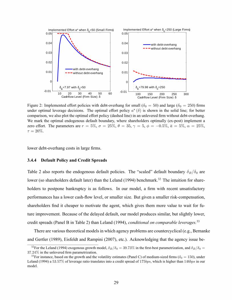
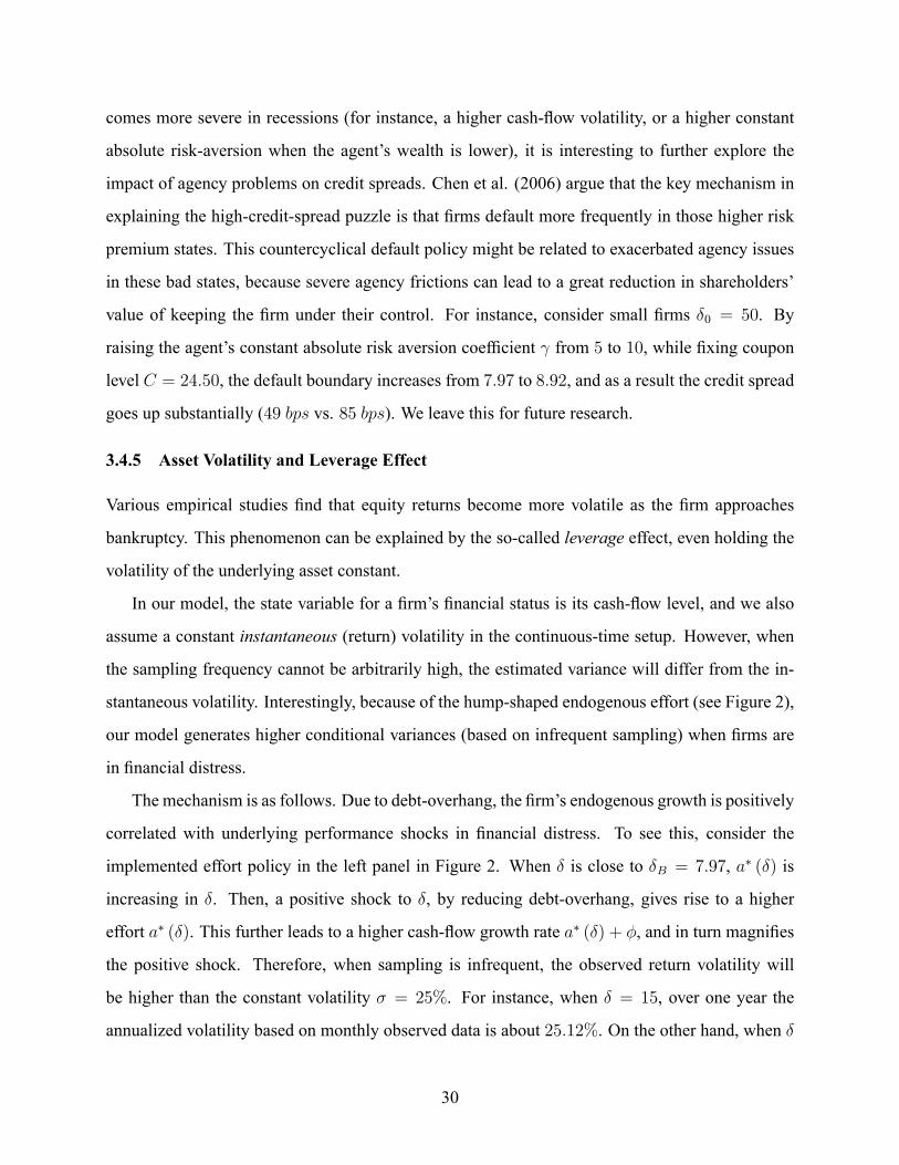
As discussed in Section 2.4.2, when the optimal effort level is interior, we have

PPS =1

1 + � r�2�t, (26)

which is decreasing in �rm size �t. Fundamentally, this result is due to the fact that as the �rm

grows, the quadratic risk-compensation cost 12 r�2a2�2�2t is in the order of �

2t , while the incentive

bene�t is in the order of �t (check (24); in Appendix A.6 we show that when �t ! 1, f 0 (�t) !1r��). This exactly re�ects the common wisdom that managers in larger �rms have lower-powered

incentive schemes due to risk considerations.21;22

Another appealing feature, which is closely related to the pattern of PPS falling in �rm size,

is that the endogenous �rm growth rate � + a�t is decreasing in �rm size �t as well (see Figure 2

in Section 3.4.3 for a numerical example). The negative relationship between �rm size and growth

is studied in, for instance, Cooley and Quadrini (2001). In this model, because incentivizing the

agent is more costly in larger �rms, the optimal contract implements a lower effort in larger �rms,

leading to a lower growth.

3.3 Optimal Employment Contract and Leverage3.3.1 Additional Assumptions

Now suppose that the �rm issues debt to take advantage of tax shields. Relative to the standard

bilateral contracting framework between investors (the principal) and the agent, now we have het-

erogenous investors�shareholders and debt holders. To abstract from complicated contracting

issues among three parties, we take the following treatment. First, the debt contract takes the form

studied in Leland (1994), i.e., only the consol bond (with a constant coupon rate C) is consid-

ered, and shareholders (with their perfectly-aligned agent when they are dealing with debt holders)21For instance, Murphy (1999) states that, �The inverse relation between company size and pay performance sen-

sitivities is not surprising, since risk-averse and wealth-constrained CEOs of large �rms can feasibly own only a tinyfraction of the company...the result merely underscores that increased agency problems are a cost of company sizethat must weighed against the bene�ts of expanded scale and scope.� Notice that under an optimal contracting frame-work, wealth-constrainedness is not an appealing justi�cation, because empirically CEOs receive a fair amount of�xed salaries in their compensation packages.22This loose reasoning is precise when the manager's risk-absorbing capacity is independent of �rm size, which

holds only for CARA preference. However, this statement is probably better interpreted as following: Even thoughthe managers in larger �rms might have greater risk-absorbing capacity (presumably because they recieve higher pay),their greater risk-absorbing capacity cannot offset the higher total risk in larger �rms. For a related discussion ofCRRA preference, see the end of Section 2.4.2.

19

can endogenously default when the �rm's �nancial status deteriorates. Second, we assume that

shareholders can ful�ll the promise of the agent's continuation value at bankruptcy as a part of

employment contract. In other words, when bankruptcy occurs, the agent is guaranteed with the

deferred-compensation fund W de�ned in (15). We will comment on this assumption in Section

3.4.2.

Another important timing assumption is that in this model, shareholders design the employment

contract as an optimal response to the leverage decision. Theoretically, this is consistent with the

fact that, in this CARA framework a long-term optimal contract can be implemented by a sequence

of short-term contracts (Fudenburg, Holmstrom, and Milgrom (1990)). Essentially, in the CARA

framework studied here, shareholders and the agent can revise the contract (as long as both parties

agree to do so) once the debt is issued,23 which generates the debt-overhang problem analyzed in

Section 3.4.2.

These assumptions represent a minimum, but essential, departure from Leland (1994). They

re�ect the key economic rationale regarding the manager's objective in US corporations: managers

are supposed to be responsible to shareholders only (Allen, Brealey, and Myers (2006)).

3.3.2 Equity Value and Endogenous Default

Similar to the case of unlevered �rms, the shareholders' value function is JE (�; V ) = fE (�) +

1 rln (� rV ). The separability between � and V hinges on the assumption that in the leveraged

�rm the shareholders can always keep the promise of delivering the continuation payoff V to the

agent, even when the �rm goes bankrupt at � = �B. In the implementation, the promise is guaran-

teed by the deferred-compensation fund which has priority over debt in the event of bankruptcy.

As in Section 2.3.4, by writing down the HJB equation for JE (�; V ), we reach the following

ODE for the equity value fE (�), where the control is over at and the bankruptcy boundary �B:

rfE (�) = maxa2[0;a];�B

�� � C (1� �) + fE0 (�) � (�+ a) � + 1

2fE00 (�)�2�2 � 1

2�a2� � 1

2 r�2a2�2�2

�,

(27)

where C is the coupon rate, and � is the corporate tax rate. The equity value fE (�) is the23In this CARA setup we allow for renegotiations in deriving the optimal contract. To see this, the resulting optimal

contract is renegotiation-proof, as the Pareto boundary is always downward-sloping, i.e., JV = 1 rV < 0 (note that

V < 0 in this model).

20

sum of (common) shareholders' value JE (�; V ), and the agent's deferred-compensation fund

� 1 rln (� rV ). Compared to (24) without debt, (27) has an additional cash out�ow C (1� �)

as the after-tax coupon payment. Similar to (25), the optimal effort is

a�t = min

�fE0 (�t)

� (1 + � r�2�t); a

�. (28)

Plugging it into (27), we have an ODE to characterize the optimal contracting.

When � falls to a certain level, say �B, shareholders refuse to serve the coupon payment by

simply declaring bankruptcy. This is captured by the value-matching boundary condition

fE (�B) = 0, (29)

and the smooth-pasting condition

fE0 (�B) = 0. (30)

Both conditions are standard in this literature (e.g., Leland (1994)). Note that these conditions

are a result of maximizing the shareholders' value JE (�; V ). But since these policies are toward

debt holders, it is equivalent to maximizing fE (�), i.e., the joint (ex-post) surplus enjoyed by

shareholders and the agent.24

For the boundary condition on the other end, when � takes a suf�ciently large value � ! 1,

the bankruptcy event is negligible. In the Appendix A.6 we show that,

fE���' f

���� C (1� �)

r; (31)

where f (�) captures the �rm value under a Gordon growth model with a growth rate � (see Eq.

(37) in the Appendix A.6), and C(1��)r

is the value for a perpetual after-tax coupon payment. Then

we can numerically solve for fE (�) and �B, based on conditions (29), (30), and (31). For detailed

numerical methods, see Appendix A.6.

3.3.3 Debt Value and Capital Structure

Given the implemented effort policy a� (�) in (28), we can evaluate the consol bond with a promised

coupon rate C. Since debt holders anticipate the optimal contracting between shareholders and the24This result implies that despite the agency con�icts between the agent and shareholders, under the optimal contract

they have perfectly aligned interests with respect to the policy toward debt holders. In other words, the default policywill not depend on whether shareholders or the agent is in charge of the bankruptcy decision. This differs fromMorellec (2004) where the agent tends to keep the �rm alive longer for more private bene�ts.

21

agent, the value of the corporate debt, D (�), satis�es:

rD (�) = C +D� (�) � (�+ a� (�)) � +1

2D�� (�)�

2�2,

with D (�B) = (1� �) f (�B) where � < 1 is the percentage bankruptcy cost, and D���! C

ras

� ! 1. Here we simply assume that, once bankruptcy occurs, debt holders pay the bankruptcy

cost �f (�B), and then keep running the project as an unlevered �rm.25

Given the time-0 cash-�ow level �0, shareholders choose coupon C to maximize the total lev-

ered �rm value fE (�0;C) + D (�0;C) before the debt issuance; they then design the optimal

contract with an agent who has an outside option v0. As discussed in Section 3.3.1, this timing

assumption is equivalent to allowing shareholders and the agent to revise the employment contract

ex-post after the debt issuance.

We de�ne the �rm's optimal leverage ratio as

LR (�0) �D (�0;C

� (�0))

fE (�0;C� (�0)) +D (�0;C� (�0)).

In Leland (1994), the scale invariance implies that the optimal leverage ratio LR is independent of

�rm size �0. However, we have seen that in our model the quadratic risk-compensation eliminates

the scale invariance. In fact, in the following calibration exercises, we will mainly investigate the

divergent leverage decisions for different-sized �rms.

3.3.4 Parameterization

Table 1 tabulates our baseline parametrization. Interest rate r = 5%, bankruptcy cost � = 25%,

and tax rate � = 20% (considering personal tax effect), are typical in the literature (e.g., Leland

(1998)).

We also record the average growth rate in the 50-year simulation, and this measure helps us

pin down � and a. In the literature with constant coef�cients, Goldstein, Ju, and Leland (2001)

calibrate a slightly negative �, and Leland (1998) chooses the growth rate � = 1%. Under the

choice of � = �0:5% and a = 5% (a is irrelevant for levered �rms as the optimal effort fa�g never

binds at 5%; see Figure 2), the simulated average growth rates �t these numbers squarely across

various �rm sizes (see Table 2).25Also, the new agent's outside option is v0 = �1

r , soW0 = 0. Our result is insensitive to the treatment of unlevered�rm after the bankruptcy.

22

Table 1: Baseline ParametersAgency Leland (1998)

Risk Aversion = 5 Volatility � = 25%

Effort Cost � = 35 Interest Rate r = 5%

Lower Bound Growth � = �0:5% Bankruptcy Cost � = 25%

Upper Bound Effort a = 5% Marginal Tax Rate � = 20%

Because in our calibration the optimal effort never binds at a in levered �rms, we have the

pay-performance sensitivity as in (26):26

PPS =1

1 + � r�2�t:

Based on this result, we choose the agency-related parameters (risk aversion = 5 which is the

median value used in Haubrich (1994), and effort cost � = 35) and the starting �rm size �0 to

match the PPS documented in the empirical literature. Jensen and Murphy (1990) report a PPS

of 0:3% in their sample (1969-1983), while Hall and Liebman (1998) document a higher PPS

with mean 2:5%. Aggarwal and Samwick (1998) control for the �rm risk, and report a mean PPS

of 6:94% from the OLS regression. For the size-dependence pattern of PPS, Murphy (1999) �nds

that for large S&P500 �rms, the PPS is approximately 1%; for Midcap �rms, it is 1:5%; and for

small �rms, it is 3%. Hall and Liebman (1998) document a mean PPS around 2:5%, and note that

in their sample, �the largest �rms (with market value over $10 billion) have a median PPS that

is more than an order of magnitude smaller than the smallest �rms (market value less than $500

million).�

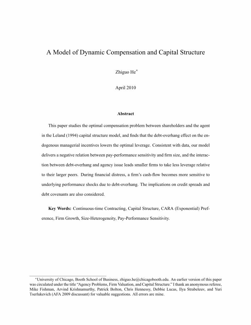
3.4 Results and Discussions3.4.1 Optimal Leverage Ratio

Because debt-overhang adversely affects the �rm's endogenous growth, relative to Leland (1994)

�rms will take less leverage for their optimal capital structure. Figure 1 shows the optimal leverage26The presence of debt does not affect the expression of PPS in (26). To see this, the agent's performance is

measured as the change of equity value fE (�). However, fE0 (�) cancels in the expression (26) when the optimaleffort a� (�) takes an interior solution (check the derivation in Eq. (20)).

23

ratio (the solid line) for �rms with different sizes. For better comparison, in Figure 1 we also pro-

vide two benchmark optimal leverage ratios predicted by the Leland (1994) model, with exogenous

constant growth. The dashed line with circles (63:21%) is the �rst-best case, where the cash-�ow

growth rate is a+ � = 4:5%. However, as we have seen in Section 3.2, the agency problem alone

reduces the �rm growth, which would lead to a lower leverage ratio even without debt-overhang.

To address this issue, we take the results of unlevered �rms from Section 3.2, simulate the model,

and obtain time-series averages of the cash-�ow growth and volatility.27 We then use these es-

timates as inputs to calculate the Leland leverage ratio, which is graphed in the dotted line with

asterisks (61:59%) in Figure 1.

The optimal leverage ratios are reported in Table 2 along with other measures. For each initial

cash-�ow level �0, we calculate the sample mean of growth and volatility of d�=� over 100 years

in 500 simulations (see Panel C in Table 1). We also report the sample average of pay-performance

sensitivity based on (26); these numbers �t the empirical estimates discussed in the last section

squarely. We �nd that for small �rms (�0 = 50), the optimal leverage ratio falls from 61:59%

(or 63:21% in the �rst-best case) to 39:35%.28 In contrast to small �rms, we �nd that the optimal

leverage ratio for large �rms is close to the result under Leland (1994), a cross-sectional result that

we will come back shortly.

3.4.2 Debt-Overhang

In Figure 1 we observe that the optimal leverage ratio is lower relative to Leland (1994). The

reason is debt-overhang, where we interpret the agent's effort as a form of �investment;� see Hen-27Speci�cally, to match the relevant range for � in levered �rms, we set the initial �0 = 250, and stop the process

once � reaches 7:97 (which is the lowest default boundary in our calibration). Also, the simulation length is 50 yearsto mitigate the impact of initial condition. We then average the time-series mean of growth rate and volatility across500 simulations, which gives an average growth rate (volatility) as 3:31% (25:02%). Other treatment gives similarresults.28This reduction is comparable to other modi�cations of the Leland (1994) benchmark. For instance, by combining

both the �callable� feature of the debt and upward capital restructuring together, Goldstein, Ju, and Leland (2001)reduce the optimal leverage from 49:8% to 37:1% in their baseline case.It is not easy to accommodate the dynamic capital restructuring into our framework, as we do not have scale-

invariance in this model. Certainly, as in Goldstein, Ju, and Leland (2001), the possibility of raising leverage in thefuture should reduce the �rm's initial leverage. In fact, dynamic capital restructuring would have an interesting impactto our model if the restructuring was downward, i.e., reducing debt when the �rm's cash �ow level drops. This isbecause in this model almost all the action is on the downside where debt overhang cuts down the ef�cient effort. Ifwe only allow for upward restructuring as in Goldstein, Ju, and Leland (2001), the interaction effect should be small.

24

50 100 150 200 2500.35

0.4

0.45

0.5

0.55

0.6

0.65

0.7

Inital Cashf low Lev el (Firm Size) δ0

Optimal Lev erage Ratio

with Agency and Debt­Overhang ProblemsLeland: First­Best CoefficientsLeland: (Simulated) Coefficients without Debt

Figure 1: Optimal leverage ratio as a function of initial cash-�ow level (�rm size). We plot the two bench-mark leverage ratios under Leland (1994). The �rst one is based on the �rst-best coef�cients (� = 4:5%and � = 25%), which gives a leverage ratio 63:21% plotted in the dashed line with circles. The secondone is based on the time-series averages in simulating the unlevered �rm in Section 3.2 (� = 3:31% and� = 25:02%; for simulation details, see footnote 27); this case yields a leverage ratio 61:59% plotted in thedotted line with asterisks. The parameters are r = 5%, � = 25%, � = 35, = 5, � = �0:5%, a = 5%,� = 25%, � = 20%.

nessy (2004) for a similar mechanism. In our model, shareholders design an employment contract

to maximize the ex-post equity value, and the smooth-pasting condition (30) implies that fE0 (�)

goes to zero as � approaches the default boundary �B. It implies that, once the �rm is close to

bankruptcy, shareholders gain almost nothing by improving the �rm's performance. Then, accord-

ing to (28) which says that the optimal effort a� is proportional to fE0 (�), shareholders implement

diminishing effort (through providing diminishing incentives) during �nancial distress. As a result,

in addition to the traditional bankruptcy cost, in our model the debt bears another form of cost due

to debt-overhang.

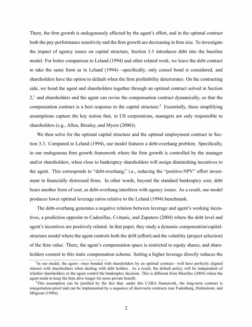
We illustrate the above mechanism in Figure 2. The left panel plots the implemented effort

investment a� in solid line as a function of �rm's �nancial status � for small �rms (�0 = 50). As

we will explain shortly, the debt-overhang problem is more severe in small �rms. We also plot the

optimal effort policy without debt-overhang (the dashed line), which corresponds to the case of

unlevered �rms studied in Section 3.2.

Relative to the effort policy without debt-overhang plotted in the dotted line, we observe an

25

Table 2: Optimal Capital Structure for Firms with Different Sizes

Initial Cash-�ow Level (Firm Size) �050 100 150 200 250

Panel A: Optimal Debt PoliciesOptimal Coupon C� 24:50 61:35 106:00 147:62 203:15

Default Boundary �B 7:97 22:79 40:58 57:28 79:98

Scaled Def. Boundary �B�0% 15:95 22:79 27:05 28:64 31:99

Panel B: Valuation and LeverageDebt Value D (�0) 446:05 997:44 1640:02 2267:70 3090:52

Lev. Ratio D(�0)D(�0)+fE(�0)

% 39:35 47:70 53:57 56:10 61:32

Credit Spreads bps 49:22 115:12 146:34 150:98 157:34

Panel C: Simulation ResultsAverage Growth % 1:95 0:50 0:12 �0:05 �0:17Average Volatility % 25:04 24:98 25:04 25:03 25:01

Pay-Perf. Sensitivity % 5:33 2:52 1:69 1:29 0:99

The parameters are r = 5%, � = 25%, � = 35, = 5, � = �0:5%, a = 5%, � = 25%, � = 20%.Credit spreads are calculated as (C=D � r)� 10000. We simulate the model for 50 years to obtain theaverage growth rate and volatility for d�=�, given the initial �0. We also calculate the agent's average pay-performance sensitivity based on (26).

abrupt drop of implemented effort when the �rm is in the verge of bankruptcy (� ! �B = 7:97).

From the view of social welfare, in this situation a higher effort is desirable, because it helps avoid

the costly bankruptcy once � hits �B. However, it is not in the shareholders' interest to ask the

agent to work hard. When the �rm approaches bankruptcy, shareholders obtain zero marginal

value from improving �. Consequently, they implement diminishing effort, a typical symptom of

debt-overhang.

We emphasize that the driving forces of the debt-overhang result are the endogenous nature

of �rm growth, and the smooth-pasting condition of the shareholders' value; both ingredients are

quite generic in practice. Therefore, if in reality the management gives place to existing share-

holders (like the board) during �nancial distress, then debt-overhang is still present without the

intermediate link of diminishing management incentives.

Leverage vs. management incentives. The debt-overhang generates a negative relation between

leverage and agent's working incentives. This result contrasts to Cadenillas, Cvitanic, and Zapatero

26

(2004), where the log agent's compensation space is restricted to equity shares, and shareholders

commit to this compensation scheme. In comparison, in our optimal dynamic contracting setup,

we do not place any restriction on the contracting space, and allow for dynamically revising the em-

ployment contract between the agent and shareholders. Finally, as we discussed in Section 3.3.1,

part of the implementation of the optimal contract requires the �rm to set the agent's deferred com-

pensation aside as cash; this way shareholders commit to fully insulate the agent's compensation

from bankruptcy. We now discuss these assumptions by relating them to �inside debt� documented

in Sundaram and Yermack (2007).

Inside debt. There are several interesting remarks regarding the above assumptions, which point

to the robustness of our debt-overhang result. First, in reality, although we do observe certain

revising activities such as resetting the strike price of executives' previously awarded options,

modifying compensation contract is not frictionless. For instance, managers' pensions�as a form

of deferred compensation�are calculated according to certain prespeci�ed formulae. More im-

portantly, these pensions represent unsecured, unfunded debt claims against �rm assets (�inside

debt� as advocated in Sundaram and Yermack (2007) and Edmans and Liu (2007)),29 rather than

a senior claim against a cash-based deferred compensation fund as in our implementation. As a

result, this portion of compensation scheme can potentially alleviate the debt-overhang problem in

this paper and the risk-shifting problem in Edmans and Liu (2009).30

Nevertheless, for �inside debt� to work, one also needs shareholders' and the agent's commit-

ment on other compensation schemes to prohibit undoing the �inside debt.� The important point is

that, to rule out ex-post revising, shareholders and the agent need �commitment� with debt holders

on all compensation schemes, rather than on one or some schemes. In other words, as long as

shareholders can modify the residual compensation freely, they can still undo the �inside-debt�,29This means that when the �rm becomes insolvent, pension bene�ciaries have the same priority as other unsecured

creditors. However, footnote 10 in Sundaram and Yermack (2007) gives an example of �secular� trust fund whichsecure an executive's pension in a bankruptcy-proof form.30These papers are closely related to the early theoretical work by John and John (1993) who consider a risk-

shifting problem. Essentially, for the agent to maximize the �rm's value, the compensation should be less alignedwith shareholders when the leverage is higher, which predicts a negative relation between leverage and PPS. There,commitment is also essential, even though it appears not so in a two-period model. In contrast, in our model, theagent is always perfectly aligned with shareholders in terms of incentives: when close to bankruptcy, even though theagent's incentives diminishes, the equity volatility vanishes in the same order as the agent's incentives, and PPS as aratio�which is always (26)�does not go to zero.

27

and theoretically we come back to the optimal contract without commitment. This implies that our

theoretical results are quite robust to the practice of �inside-debt.� And, there is some indirect em-

pirical evidence consistent with this view of �undoing� or �dynamically revising� the employment

contract, which can be a potential topic for future empirical studies.31

3.4.3 Size-Heterogeneity

Our model offers another explanation why small �rms take less leverage relative to their large

peers, a stylized fact documented in the literature (e.g., Frank and Goyal (2005)). The mechanism

here is rooted in divergent severities of the aforementioned debt-overhang problem for different

sized �rms. In this model, to be consistent with the inverse relation between PPS and �rm size,

larger �rms implement lower effort. This implies that, for larger �rms, debt-overhang�which

reduces the pro�table effort investment�is less of concern. Consequently, larger �rms will issue

more debt to maximize the ex-ante �rm value.

This point is illustrated in the right panel in Figure 2, where we plot the same effort policies with

and without debt-overhang for large �rms (�0 = 250). For better comparison, the right panel adopts

the same scale as the left panel where small �rms are considered. We �nd that debt-overhang

becomes moderate for large �rms. As shown, at their relatively high default boundary �B = 79:98,

the optimal effort even without debt-overhang is quite low (only about 1:14%). Therefore, the drop

of a�t when larger �rms approach bankruptcy�the exact force of debt-overhang�is less dramatic

compared to smaller �rms (the left panel). In sum, in smaller �rms the debt-overhang cost is

greater, leading to a lower predicted leverage ratio.

It is important to add that this result is not driven by CARA preference. Rather, we only

use CARA preference as the analytical tool to match the empirical pattern of pay-performance

sensitivity (PPS), and it is the negative relationship between PPS and �rm size that implies31Bryan, Hwang, and Lilien (2000) analyze the Incentive-Intensity (the change in the value of annual stock-based

compensation per change in equity value) andMix (ratio of the value of annual stock-based compensation to cash com-pensation) measures, which are based on the annual stock-based grants only (as opposed to cumulative inside holdingswhich relate to the agent's �wealth�). Interestingly, they �nd that both Incentive-Intensity and Mix decrease with �rmleverage. Under the debt-overhang framework studied in this paper, to the extent that working incentives generated by�inside debt� is increasing with leverage, these empirical result is consistent with the dynamic revising activity. Also,decreasing Mix with leverage implies that �nancially troubled �rms pay the agent more cash compensation, a resultconsistent with our model if the juniority of pensions force the �rm to start paying out deferred compensation to theagent in the form of cash.

28

10 20 30 40 50 60­0.01

0

0.01

0.02

0.03

0.04

0.05

Cashflow Level (Firm Size) δ

Implemented Effort a* when δ0=50 (Small Firms)

100 150 200 250 300­0.01

0

0.01

0.02

0.03

0.04

0.05

Cashflow Level (Firm Size) δ

Implemented Effort a* when δ0=250 (Large Firms)

with debt­overhangwithout debt­overhang

with debt­overhangwithout debt­overhang

δB=7.97 with δ

0=50 δ

B=79.98 with δ

0=250

Figure 2: Implemented effort policies with debt-overhang for small (�0 = 50) and large (�0 = 250) �rmsunder optimal leverage decisions. The optimal effort policy a� (�) is shown in the solid line; for bettercomparison, we also plot the optimal effort policy (dashed line) in an unlevered �rm without debt-overhang.We mark the optimal endogenous default boundary, where shareholders optimally (ex-post) implement azero effort. The parameters are r = 5%, � = 25%, � = 35, = 5, � = �0:5%, a = 5%, � = 25%,� = 20%.

lower debt-overhang costs in large �rms.

3.4.4 Default Policy and Credit Spreads

Table 2 also reports the endogenous default policies. The �scaled� default boundary �B=�0 are

lower (so shareholders default later) than the Leland (1994) benchmark.32 The intuition for share-

holders to postpone bankruptcy is as follows. In our model, a �rm with recent unsatisfactory

performances has a lower cash-�ow level, or smaller size. But given a smaller risk-compensation,

shareholders �nd it cheaper to motivate the agent, which gives them more value to wait for fu-

ture improvement. Because of the delayed default, our model produces similar, but slightly lower,

credit spreads (Panel B in Table 2) than Leland (1994), conditional on comparable leverages.33

There are various theoretical models in which agency problems are countercyclical (e.g., Bernanke

and Gertler (1989), Eisfeldt and Rampini (2007), etc.). Acknowledging that the agency issue be-32For the Leland (1994) exogenous growth model, �B=�0 = 39:73% in the �rst-best parametrization, and �B=�0 =

37:24% in the unlevered �rm parametrization.33For instance, based on the growth and the volatility estimates (Panel C) of medium-sized �rms (�0 = 150), under

Leland (1994) a 53:57% of leverage ratio translates into a credit spread of 175bps, which is higher than 146bps in ourmodel.

29

comes more severe in recessions (for instance, a higher cash-�ow volatility, or a higher constant

absolute risk-aversion when the agent's wealth is lower), it is interesting to further explore the

impact of agency problems on credit spreads. Chen et al. (2006) argue that the key mechanism in

explaining the high-credit-spread puzzle is that �rms default more frequently in those higher risk

premium states. This countercyclical default policy might be related to exacerbated agency issues

in these bad states, because severe agency frictions can lead to a great reduction in shareholders'

value of keeping the �rm under their control. For instance, consider small �rms �0 = 50. By

raising the agent's constant absolute risk aversion coef�cient from 5 to 10, while �xing coupon

level C = 24:50, the default boundary increases from 7:97 to 8:92, and as a result the credit spread

goes up substantially (49 bps vs. 85 bps). We leave this for future research.

3.4.5 Asset Volatility and Leverage Effect

Various empirical studies �nd that equity returns become more volatile as the �rm approaches

bankruptcy. This phenomenon can be explained by the so-called leverage effect, even holding the

volatility of the underlying asset constant.

In our model, the state variable for a �rm's �nancial status is its cash-�ow level, and we also

assume a constant instantaneous (return) volatility in the continuous-time setup. However, when

the sampling frequency cannot be arbitrarily high, the estimated variance will differ from the in-

stantaneous volatility. Interestingly, because of the hump-shaped endogenous effort (see Figure 2),

our model generates higher conditional variances (based on infrequent sampling) when �rms are

in �nancial distress.

The mechanism is as follows. Due to debt-overhang, the �rm's endogenous growth is positively

correlated with underlying performance shocks in �nancial distress. To see this, consider the

implemented effort policy in the left panel in Figure 2. When � is close to �B = 7:97, a� (�) is

increasing in �. Then, a positive shock to �, by reducing debt-overhang, gives rise to a higher

effort a� (�). This further leads to a higher cash-�ow growth rate a� (�) + �, and in turn magni�es

the positive shock. Therefore, when sampling is infrequent, the observed return volatility will

be higher than the constant volatility � = 25%. For instance, when � = 15, over one year the

annualized volatility based on monthly observed data is about 25:12%. On the other hand, when �

30

is far away from the bankruptcy threshold, a� (�) is decreasing in �, and the exact opposite force

leads to a lower volatility estimate (when � = 50, the above mentioned annualized volatility is

about 24:68%).

In sum, in our model, for a �rm near bankruptcy, its �nancial status becomes more sensitive

to underlying performance shocks. In fact, this general message does not depend on the discrete-

sampling, as in our model the �rm value (rather than the instantaneous cash �ow rate) displays a

higher instantaneous volatility during �nancial distress.34

3.4.6 Debt Covenants

A commonly observed debt covenant is that debt holders can force shareholders to go bankrupt

when the �rm's cash-�ow � hits a prespeci�ed level �bB. This covenant is along the same line as

�positive net-worth covenants for protected debt� in Leland (1994) which stipulates that the �rm

defaults whenever the asset value drops to the debt face value. Under our cash-�ow framework,

this can also be interpreted as a hard covenant on the interest coverage ratio, which, combined with

coupon C, gives the bankruptcy threshold.35

In the standard trade-off model as in Leland (1994), a forced earlier default always hurts �rm

value, because an earlier default reduces the tax bene�t and raises the bankruptcy cost. In fact, if

equity holders can fully commit in Leland (1994), then �no default� is the �rst-best outcome.

In contrast, due to the debt-overhang problem, in our model specifying �bB > �B might be

welfare improving. The reason is that now around �bB, we no longer have the smooth-pasting

condition as in (30), and shareholders will bene�t from improving the �rm performance. Then,

specifying �bB > �B is equivalent to committing to provide incentives (to the agent) even in the

deep �nancial distress, and it might be socially optimal to do so. For instance, for small �rms

�0 = 50, given the coupon C = 24:50, the optimal �bB = 8:05 > �B = 7:97, and the �rm value

becomes 1133:81 > 1133:67. Though small magnitude, this interesting �nding distinguishes our34The �rm's asset value, generated by future cash-�ows, can be de�ned as X (�t) =

EthR �(�=�B)

te�r(s�t)�sds+ f (�B)

i, where � (� = �B) is the �rst passage time of � hitting �B . Then, the

instantaneous return volatility of X (�t) will be larger when �t is close to �B . The reason is that X (�t) takes intoaccount the impact on the stochastic growth �, which positively correlates with �t during distress.35Because part of the coupon C can be interpreted as constant operating cost (in other words, the leverage derived

here includes operating leverage too), the effective interest coverage ratio can be much higher than implied by �bB=C.

31

model from Leland (1994) and its variations where the �rm growth is exogenously speci�ed.

4 Concluding Remarks

By generalizing the optimal contracting result to widely-used cash-�ow setups in �nance, this

paper offers a more tractable framework to investigate the impact of agency problems in various

economic contexts. The absence of wealth effect due to CARA preference simpli�es the optimal

contracting problem with private savings, and we characterize the optimal contract by an ODE.

When we apply our results to the geometric Brownian cash-�ow setup as a revisit to Leland (1994),

the underinvestment of effort due to debt-overhang produces a lower optimal leverage ratio, and

the interesting interaction between agency issue and debt-overhang leads smaller �rms to take less

debt in their leverage decisions.

The relatively simple structure in this paper leaves several directions for future research. For

instance, incorporating investment decisions would be desirable, as one can explore the invest-

ment distortion and its interaction with �nancing decisions under agency problems. Also, incor-

porating time-varying risk premia which is correlated with agency frictions (e.g., time-varying

risk-aversion) will be valuable to investigate the agency impacts on credit spreads.

ReferencesAggarwal, R., and A. Samwick, 1999, �The Other Side of the Tradeoff: The Impact of Risk on ExecutiveCompensation,� Journal of Political Economy 107, 65-105.

Allen, F., S. Myers, and R. Brealey, 2006, �Principles of Corporate Finance,� 8th Edition, New York, McGraw-Hill/Irwin.

Baker, G., and B. Hall, 2004, �CEO incentives and Firm Size,� Journal of Labor Economics 22, 767-798.

Bernanke, B., andM. Gertler, 1989, �Agency Costs, NetWorth, and Business Fluctuations,� American EconomicReview 79, 14-31.

Biais, B., T. Mariotti, G. Plantin, and J. Rochet, 2007, �Dynamic Security Design: Convergence to ContinuousTime and Asset Pricing Implications,� Review of Economic Studies 74, 345-390.

Bryan, S., L. Hwang, and S. Lilien, 2000, �CEO Stock-Based Compensation: An Empirical Analysis ofIncentive-Intensity, Relative Mix, and Economic Determinants,� Journal of Business 73, 661-693.

Cadenillas, A., J. Cvitanic, and F. Zapatero, 2004, �Leverage Decision and Manager Compensation with Choiceof Effort and Volatility,� Journal of Financial Economics 73, 71-92.

32

Chen, L., P. Collin-Dufresne, and R. Goldstein, 2006, �On the Relation between the Credit Spread Puzzle andthe Equity Premium Puzzle,� Working Paper, U.C. Berkeley.

Cheung, Y., and L. Ng, 1992, �Stock Price Dynamics and Firm Size: An empirical Investigation,� Journal ofFinance 47, 1985-1997.

Cooley, T., and V. Quadrini, 2001, �Financial Markets and Firm Dynamics,� American Economic Review 91,1286-1310.

DeMarzo, P., and M. Fishman, 2006, �Optimal Long-Term Financial Contracting,� forthcoming in Review ofFinancial Studies.

DeMarzo, P., and Y. Sannikov, 2006, �Optimal Security Design and Dynamic Capital Structure in a Continuous-Time Agency Model,� Journal of Finance, 61, 2681-2724.

Edmans, E. and Q. Liu, 2008, �Inside Debt,� forthcoming in Review of Finance.

Edmans, A., X. Gabaix, and A. Landier, 2007, �A Calibratable Model of Optimal CEO incentives in MarketEquilibrium,� Working paper, Wharton and NYU.

Edmans, A., X. Gabaix, T. Sadzik, and Y. Sannikov, 2009, �Dynamic Incentive Accounts,� Working paper,Wharton, NYU, and Princeton.

Eisfeldt, A. and A. Rampini, 2007, �Managerial Incentives, Capital Reallocation, and the Business Cycle,�forthcoming in Journal of Financial Economics.

Frank, M. and V. Goyal, 2005, �Trade-off and Pecking Order Theories of Debt,� Handbook of Corporate Fi-nance: Empirical Corporate Finance, Chapter 7, edited by B, Eckbo, Elsevier/North-holland, 2005.

Fudenberg, D., B. Holmstrom, and P. Milgrom, 1990, �Short-Term Contracts and Long-Term Agency Relation-ships,� Journal of Economic Theory 51, 1-31.

Gabaix, X., and A. Landier, 2008, �Why Has CEO Pay Increased So Much?� Quarterly Journal of Economics.

Goldstein R., N. Ju, and H. Leland, 2001, �An EBIT-Based Model of Dynamic Capital Structure,� Journal ofBusiness 74, 483-512.

Hall, B., and J. Liebman, 1998, �Are CEOs Really Paid Like Bureaucrats?� Quarterly Journal of Economics113, 653-69.

Haubrich, J., 1994, �Risk Aversion, Performance Pay, and the Principal-Agent Problem,� Journal of PoliticalEconomy 102, 258-276.

He, Z., 2009, �Optimal Executive Compensation when Firm Size Follows Geometric Brownian Motion,� Reviewof Financial Studies 22, 859-892.

He, Z., 2010, �Dynamic Compensation Contracts with Private Savings,� Working Paper, University of Chicago.

Hennessy, C., 2004, �Tobin's Q, Debt Overhang, and Investment,� Journal of Finance 59, 1717-1742.

33

Holderness, C., R. Kroszner, and D. Sheehan, 1999, �Were the Gold Old Days That Good? Changes in Man-agerial Stock Ownership Since the Great Depression,� Journal of Finance 54, 435-469.

Holmstrom, B., and P. Milgrom, 1987, �Aggregation and Linearity in the Provision of Intertemporal Incentives,�Econometrica 55, 303-328.

Jensen, M., and K. Murphy, 1990, �Performance Pay and Top-management Incentives,� Journal of PoliticalEconomy 98, 225-264.

John, T., and K. John, 1993, �Top-Management Compensation and Capital Structure,� Journal of Finance 48,949-974.

Leland, H., 1994, �Corporate Debt Value, Bond Covenants, and Optimal Capital Structure,� Journal of Finance49, 1213-1252.

Leland, H., 1998, �Agency Costs, Risk Management, and Capital Structure,� Journal of Finance 53, 1213-1243.

Morellec, E., 2004, �Can Managerial Discretion Explain Observed Leverage Ratios?� Review of Financial Stud-ies 17, 257-294.

Murphy, K., 1999, �Executive Compensation�, in Orley Ashenfelter and David Card (eds.), Handbook of LaborEconomics, Vol. 3, North Holland.

Piskorski, T., and A. Tchistyi, 2007, �Optimal Mortgage Design�, Working paper, NYU.

Rogerson, W., 1985, �Repeated Moral Hazard,� Econometrica 53, 69-76.

Sannikov, Y., 2008, �A Continuous-Time Version of the Principal-Agent Problem,� Review of Economic Studies75, 957-984.

Schattler, H., and J. Sung, 1993, �The First-Order Approach to the Continuous-Time Principal-Agent Problemwith Exponential Utility,� Journal of Economic Theory 61, 331-371.

Strebulaev, I. A., 2007, �Do Tests of Capital Structure Theory Mean What They Say?� Journal of Finance 62,1747-1787.

Subramanian, A., 2007, �Managerial Flexibility, Agency Costs and Optimal Capital Structure,� Working Paper,Georgia State University.

Sundaram, R., and D. Yermack, 2007, �Pay Me Later: Inside Debt and Its Role in Managerial Compensation,�Journal of Finance 62, 1551-1587.

Wester�eld, M., 2006, �Dynamic Contracts with Hidden Actions in Continuous Time,� Working Paper, USC.

Williams, N., 2006, �On Dynamic Principal-Agent Problems in Continuous Time,� Working Paper, Princeton.

34

A Appendix

A.1 Proof of Lemma 2Consider any contract� = fc; ag which induces an optimal policy fbc;bag from the agent with a value bV0. Fromthe agent's budget equation, we have

St =R t0er(t�s) (cs � bcs) ds;

which gives the agent's optimal savings path, with the transversality condition limT!1

E [e�rTST ] = 0. Note thatthe transversality condition holds for all measures induced by any feasible effort policies.

By invoking the replication argument similar to revelation principle, we consider giving the agent a directcontract b� = fbc;bag; notice that shareholders have the same cost to deliver this contract as � = fc; ag. Clearlytaking consumption-effort policy fbc;bag is feasible for the agent with no private-savings. We need to show thatfbc;bag is indeed optimal for the agent. Suppose that given the contract b�, the agent �nds that fc0; a0g yields astrictly higher payoff V 0

0 >bV0 in problem (2), with associated savings path

S0t =R t0er(t�s) (bcs � c0s) ds;

which satis�es transversality condition. However, consider the following saving path

S00t = St + S0t =

R t0er(t�s) (cs � c0s) ds;

which also satis�es the transversality condition. But this implies that given the original contract �, the savingrule S00t supports fc0; a0g but delivering a strictly higher payoff V 0

0 . This contradicts with the optimality of fbc;bagunder the contract �.

A.2 Proof of Lemma 3Given any savings St = S and a contract � = fc; ag, from time-t on the agent's problem is (recall problem(2))

maxfbcsg,fbasg E

�Z 1

t

�1 e� (bcs�g(�s;bas))�r(s�t)ds

�(32)

s:t: dSs = rSsds+ csds� bcsds; St = S; s > td�s = � (�s;bas) ds+ � (�s) dZs:

Denote by fbc�s;ba�sg the solution to the above problem, and by Vt (�; S) the resulting agent's value.Now consider the problem with S = 0, which is the continuation payoff along the equilibrium path:

maxfbcsg,fbasg E

�Z 1

t

�1 e� (bcs�g(�s;bas))�r(s�t)ds

�s:t: dSs = rSsds+ csds� bcsds; St = 0; s > t

d�s = � (�s;bas) ds+ � (�s) dZs:We claim that the solution to this problem is fbc�s � rS;ba�sg, and therefore the value is Vt (�; 0) = e rSVt (�; S).There are two steps to show this. First, this solution is feasible. Second, suppose that there exists another policy

35

fbc0s;ba0sg that is superior to fbc�s � rS;ba�sg, so that the associated value V 0t (�; 0) > e

� rSVt (�; S). Considerfbc0s + rS;ba0sg, which is feasible to the problem (32). But under this plan the agent's objective is

e� rS �maxEt�Z 1

t

�1 e� (bc0s�g(�s;ba0s))�r(s�t)ds

�= e� rSV 0

t (�; 0) > Vt (�; S) :

which contradicts with the optimality of fbc�s;ba�sg. As a result, Vt (�; S) = e� rSVt (�; 0).A.3 Appendix for Section 2.3.4A.3.1 An Example: Square-Root Mean-Reverting Cash-Flows

Suppose that � (�t; at) = (�� ��t) + at�t, and � (�t) = �p�t, where �, �, and � are positive constants.

The agent's effort cost g (�; a) = �2a2� which is quadratic in effort and linear in the cash-�ow level. We have

�t =ga(�t;at)

�a(�t;at)= �a, and the risk-compensation is linear in �rm size �:

1

2 r

�ga (�t; at)� (�t)

�a (�t; at)

�2=1

2 r�2a2�2�.

Since all elements in (12) are af�ne in �, we guess that the �rm value f (�) = A+B�, where A and B areconstants to be determined. Focusing on the interior solution, we have A = B�

r, and

B =2

r + �+q(r + �)

2 � 2(1+� r�2)�

.

In the optimal contract, the constant optimal effort a� is

a� =B

� (1 + � r�2).

The evolutions of the agent's wage (consumption) policy follows (8), and the agent's continuation value isgoverned by

dVt = r (�Vt)B�p�t

1 + � r�2dZt. (33)

This example gives a counterpart of Holmstrom and Milgrom (1987) who derive a constant optimal effort in aGaussian framework.

We can solve Eq. (33) to obtain:

Vt = V0 exp

��Z t

0

1

2 2r2�2a�2�2�sds�

Z t

0

r�a��p�tdZs

�< 0:

One can show that if (�� a�)2 � 2M2�2 where M 2 = 12 2r2�2a�2�2, then fV g is a indeed martingale.

The proof is available upon request. Whenever the expression of Vt is needed, we will focus on this case in thefollowing analysis.

36

A.3.2 Veri�cation of Optimality of Contract

Now we verify that the optimal contract derived above is indeed optimal. As usual, we denote by c (a) therecommended consumption (effort), and bc (ba) is the agent's actual policies. The main argument applies to moregeneral cases, with case-by-case technical requirement to ensure the transversality conditions.

Step 1. We show that the agent's policy stated in Section 2.3.3 is optimal, i.e., the contract is indeedincentive compatible and induce no savings. Given arbitrary policies fbc;bag, consider the following auxiliarygain process

GAt =

Z t

0

e� (bcs�g(bas))�rs

ds+ e�rte� rStVt;

where St =R t0er(t�s) (cs � bcs) ds is the agent's cumulative (deviation) wealth, and

dVt = �a� (� rVt) [d�t � � (�t; a�t ) dt]

according to the optimal contract. Then

e rStertdGAt =e� (bct�g(bat))

e rStdt� rVtdt+ r (rSt + ct � bct)Vtdt (34)

+�a� (� rVt)h(�� (�� bat) �t) dt+ �p�tdZt � � (�t; a�t ) dti :

We aim to show that Et [e rStertdGAt ] is zero under optimal contract, while nonpositive for other policies. First,it is easy to see that the RHS of Eq. (34) (with control variables bct and bat) is a well-de�ned concave problem,with FOC as

bct : �e� (bct�g(bat))

e rSt � rVt = 0;

bat : �e� (bct�g(bat))e rSt�bat�t + �a� (� rVt) �t = 0:These two conditions imply that the RHS of Eq. (34) takes its maximum value when bat = a0 = a�, and bct = c0(here we denote by c0 and a0 as the agent's optimal policies) such that

�e� (c0�g(a�))

e rSt = rVt:

Since in the optimal contract rVt = u (ct; a�) = e� (ct�g(a�))

, we have

c0 = rSt + ct;

which says that from time-t on it is optimal to consume future wages c and permanent interest income earnedfrom today's private wealth rSt. Plugging these results into Eq. (34), we have

e rStertdGAt = non-positive drift+ �a� (� rVt)�

p�tdZt, (35)

and when the agent takes the recommended effort and consumption policy the drift is zero.

Eq. (35) implies that E [GAT ] � GA0 +Z T

0

e�rte� rSt�a� (� rVt)�p�tdZt, for 8T . As usual, we impose

extra conditions on feasible St so that the second term is indeed a martingale (when St = 0 along the equilibrium

37

path, it isZ T

0

e�rtdVt, which is a martingale since fV g is a martingale.) Because GA0 = V0, then the value

from an arbitrary feasible policy delivers a value below V0, i.e.,

E�Z 1

0

e� (bcs�g(bas))�rs

ds

�� V0;

provided that the transversality condition EhlimT!1

e�rT e� rSTVT

i= 0 holds. When St = 0 along the equilib-

rium path, V is a martingale and therefore this transversality condition follows trivially.Step 2. Now we verify the optimality of shareholders' policy. De�ne the shareholders' gain process as

GIt =

Z t

0

e�rs (�s � cs) ds+ e�rtJ (�t; Vt)

where J (�t; Vt) = B�r+B�t +

ln(� rVt) r

. Due to construction, under any employment contract we have

dGIt = aGIdt+ e�rt (B � �t)�p�dZt:

It is easy to show that due to construction, aGI is nonpositive, and zero under the optimal contract. we impose ausual square-integrable condition on feasible employment contracts:

E�Z T

0

e�rt�2t�2�tdt

�<1 for 8T (36)

Notice that in the optimal contract, �t is the constant �a�; therefore the optimal contract satis�es condition (36),

and E�Z T

0

e�rtGIt

�= 0 for all T .

Finally we check the shareholders' transversality condition EhlimT!1

e�rTJ (�T ; VT )i= 0. Under the

optimal contract, since � is stationary, we only have to check the term associated with VT . But

ln (�VT ) r

= Constant�Z T

0

1

2 2r2�2a�2�2�tdt+

Z T

0

r�a��p�tdZt;

and again the second diffusion term is a martingale given the condition (�� a�)2 � 2M 2�2 (the proof is

available upon request.) Because E�Z T

0

�tdt

�is in the order of T when T ! 1 as the long-run mean of �t

is ���a� , transversality condition holds for the optimal contract. For general policies, notice that J (�T ; VT ) �

BFB�r

+BFB�T +ln(� rVT )

rwhich is the �rst-best result. Because � is mean-reverting, the suf�cient condition

is EhlimT!1

e�rT ln(� rVT ) r

i� 0, which is the condition that we impose in addition to (36) for any feasible

contract �.

A.4 Appendix for Section 3.1We have rAFB = max

a2[0;a]

�1 +AFB (�+ a)� �

2a2, and are interested in characterizing the condition for

the �rst-best effort aFB to bind at a. When a takes an interior solution, then a� = AFB

�, and AFB =

2

r��+p(r��)2� 2

�

. First, we need to ensure that (r � �)2 > 2�so that AFB is real; otherwise the �rm value

is unbounded, resulting in an unbounded aFB . Therefore, when (r � �)2 � 2�, aFBt = a. Second, even

when (r � �)2 > 2�, it is possible that the implied the �rst-best effort 1

�2

r��+p(r��)2� 2

�

> a. In this case, the

�rst-best effort also binds at aFBt = a. Under both scenarios, AFB = 1� �2a

2

r���a .

38

A.5 Appendix for Section 3.2Under the boundary conditions speci�ed in Section 3.2, f 0 is always positive in (24), therefore a� never binds atzero in this problem. To see this, clearly f 0 (0) > 0 (notice f (0) = 0, and for � > 0, even with zero effort (sowithout the agent) the value is positive). When when � !1, using (24) and (25) one can check that

f (�) ' f (�) � 1

r � �� +1

2 (r � �)2 �2 r�2. (37)

which is increasing in �. Now suppose that there exists �1 > 0 such that f 0 (�1) = 0; take the smallest oneso that f 00 (�1) < 0. Therefore we have rf (�1) = �1 +

12f 00 (�1)�

2�21 < �1. But there must exists anotherpoint �2 > �1, such that f is deceasing in [�1; �2], and f becomes increasing again after �2 (as f is increasingwhen � is large enough). This implies f (�2) < f (�1), f 0 (�2) = 0 and f 00 (�2) > 0. But (24) implies thatrf (�2) > �2 > �1 > rf (�1), contradiction with f (�2) < f (�1).

A.6 Appendix for Section 3.3.2When � ! 1, the probability of bankruptcy is negligible, and the �rm value can be viewed as the unlevered�rm value minus the present value of after-tax coupon payment. Eq. (37) gives the unlevered �rm value fwhen � ! 1; notice that f 0 approaches to 1

r�� similar to the standard Gordon growth model. ThereforefE (�) ' f (�)� (1��)C

rwhen � is suf�ciently large.

There is one technical issue under this geometric Brownian motion setup. As illustrated in Appendix A.3, werequire that the agent's continuation value V de�ned in (10) is indeed a martingale. Unfortunately, if � followsan unbounded geometric Brownian motion, we are unable to verify that fV g is martingale. To circumvent thistechnical issue, we simply assume that when the �rm's � reaches a suf�ciently large �, shareholders simply sellthe �rm at a price f

���, and the employment contract terminates once this upper threshold is reached. This

simplifying assumption can be interpreted as an successful exit option (e.g., M&A) in reality, and has no impacton the static capital structure decision at date 0. Finally, once the state space becomes bounded, following theargument in Section A.3 one can easily show the optimality of the contract.

We use Matlab built-in solver bvp4c to solve the model, setting the tolerance level to be 10�8. We set� = 500. In solving for the bankruptcy boundary �B , we �rst choose one candidate �1B , and solve fE based on(29), (30), and (31) using bvp4c. Then we evaluate fE0

��1B�; if fE0

��1B�>(<)0 which means that �1B is too

low (high), we adjust �1B upward (downward). We use a bisection method to search for �B , which convergesrather quickly.

39