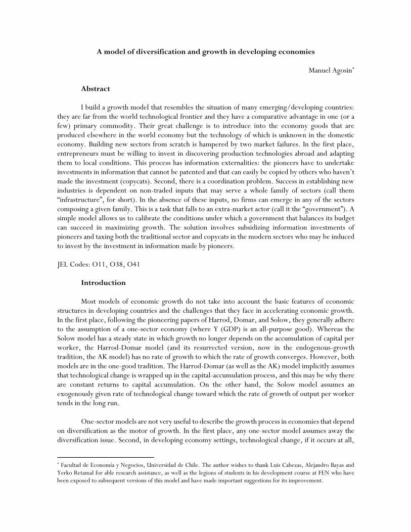
A Model of Diversification and Growth in Developing Economies

Autor:

Manuel Agosin

Santiago, Noviembre de 2017

SDT 455

A model of diversification and growth in developing economies

Manuel Agosin*

Abstract I build a growth model that resembles the situation of many emerging/developing countries: they are far from the world technological frontier and they have a comparative advantage in one (or a few) primary commodity. Their great challenge is to introduce into the economy goods that are produced elsewhere in the world economy but the technology of which is unknown in the domestic economy. Building new sectors from scratch is hampered by two market failures. In the first place, entrepreneurs must be willing to invest in discovering production technologies abroad and adapting them to local conditions. This process has information externalities: the pioneers have to undertake investments in information that cannot be patented and that can easily be copied by others who haven’t made the investment (copycats). Second, there is a coordination problem. Success in establishing new industries is dependent on non-traded inputs that may serve a whole family of sectors (call them “infrastructure”, for short). In the absence of these inputs, no firms can emerge in any of the sectors composing a given family. This is a task that falls to an extra-market actor (call it the “government”). A simple model allows us to calibrate the conditions under which a government that balances its budget can succeed in maximizing growth. The solution involves subsidizing information investments of pioneers and taxing both the traditional sector and copycats in the modern sectors who may be induced to invest by the investment in information made by pioneers. JEL Codes: O11, O38, O41

Introduction

Most models of economic growth do not take into account the basic features of economic structures in developing countries and the challenges that they face in accelerating economic growth. In the first place, following the pioneering papers of Harrod, Domar, and Solow, they generally adhere to the assumption of a one-sector economy (where Y (GDP) is an all-purpose good). Whereas the Solow model has a steady state in which growth no longer depends on the accumulation of capital per worker, the Harrod-Domar model (and its resurrected version, now in the endogenous-growth tradition, the AK model) has no rate of growth to which the rate of growth converges. However, both models are in the one-good tradition. The Harrod-Domar (as well as the AK) model implicitly assumes that technological change is wrapped up in the capital-accumulation process, and this may be why there are constant returns to capital accumulation. On the other hand, the Solow model assumes an exogenously given rate of technological change toward which the rate of growth of output per worker tends in the long run. One-sector models are not very useful to describe the growth process in economies that depend on diversification as the motor of growth. In the first place, any one-sector model assumes away the diversification issue. Second, in developing economy settings, technological change, if it occurs at all,

* Facultad de Economía y Negocios, Universidad de Chile. The author wishes to thank Luis Cabezas, Alejandro Bayas and Yerko Retamal for able research assistance, as well as the legions of students in his development course at FEN who have been exposed to subsequent versions of this model and have made important suggestions for its improvement.

2

is the result of factors of production moving from less productive to more productive uses in new sectors that didn’t exist previously. In fact, I would venture that much that is measured as technical change in developing countries is related to the introduction of new sectors which involve higher factor productivities and results from the diversification of production. In the view of development offered by Hausmann and Rodrik (2003), growth in developing countries is the result of self-discovery, which involves the incorporation of sectors that are new to the domestic economy but which exist elsewhere. Since these new sectors have higher factor productivities, measured technical change (or “total factor productivity”) reflects the shift of resources from lower- to higher productivity sectors.

Technical change, in the sense of most of the growth literature, has no place in models based on “self-discovery”. In these, the key to growth is the process by which goods produced elsewhere in the world economy are incorporated into specific developing country settings. The technology thus acquired is new to the recipient but not new to the world.

Self-discovery involves copying technologies that cannot be patented rather than adding new

products or technologies to the stock of world knowledge. This way of looking at development is a close cousin to Gerschenkron’s (1962) “advantages of backwardness”. Hausmann and Rodrik (2003) identify two reasons why the amount of self-discovery (i.e., the pace at which goods and technologies extant in the world economy are incorporated into a developing country setting) is sub-optimal. In the first place, the discovery that a product can be produced with comparative advantage in a specific country generates important informational externalities. In other words, the pioneers who make the investment in information may be unable to appropriate the entire return on their investment, because others can readily copy it. However, copying is key to the social benefits of the investment in information.

Second, there is a coordination externality. Any de novo endeavor involves the need to

coordinate the activities of many actors, some private, others public. In particular, the production of any new good will require the existence of non-tradable infrastructure. Think of exploiting a new mine. For exports to take place, roads and a port have to be built. Or of producing any new agricultural good for export: it requires phytosanitary controls to enable exports, transport links from producer to port, cold-storage facilities, knowledge of who the buyers are and the tastes of foreign consumers.

We place particular importance on exports, because we will be attempting to disentangle the

conditions under which developing countries can begin to produce goods already in existence in the world economy and do so with comparative advantage; (eventually) unaided exports are the best evidence of comparative advantage.

I. Some recent literature There hasn’t been a great volume of literature, either theoretical or empirical, emphasizing the

role that diversification of production and exports can play in the economic growth of countries well below the world technological frontier. Mention has been made of the paper by Hausmann and Rodrik (2003). An older contribution is Lucas (1993), which emphasizes learning by doing as a source of growth in developing economies. The gist of his paper is modeling the path of an economy that is not initially competitive but is able to become so through learning by doing. Lucas’ mechanism for learning by doing is the accumulation of human capital, which has a kinship to the model I develop below.

3

However, Lucas’s is still a one-sector model and, therefore, doesn’t capture the basic stylized fact that growth is associated with diversification.

The growth driver in both Rosenstein-Rodan’s classic 1943 paper and its formalization by

Murphy, Schleifer, and Vishny (1989) is the domestic market and the pecuniary external economies of investment in various sectors jointly. The emphasis on coordination externalities also has a certain resonance in this paper, which, however, has no place for domestic demand. The externalities involved here are those that relate to information useful in producing new goods, and the coordination that is necessary is at the level of efficient supply, not aggregate demand.

One study, by Imbs and Wacziarg (2003), show that countries that have higher incomes become

more diversified in both exports and output, but up to a point in their growth process, after which concentration begins to rise again. Our interest is the inverse of the relationship explored by Imbs and Wacziarg: we are interested in whether diversification of output and exports leads to higher growth. This issue is explored empirically by Hesse (2009), who finds that, with the use of panel data and a GMM econometric technology, indeed, countries that diversify their exports tend to grow more rapidly than those that do not. In addition, Hausmann and several colleagues show that initial diversification of exports leads to subsequent higher economic growth (see, for example, Hausmann, Hwang, and Rodrik, 2006; and Hausmann and Klinger, 2006).

II. The setup

The model I develop and simulate in this paper explicitly accounts for the centrality of

diversification in economic growth in countries at low levels of initial income. In keeping with the modest capabilities for innovation in most developing countries, I assume that there is no total factor productivity growth and no variable reflecting productivity. Instead, the “growth driver” in the model is the introduction into the economy of production functions from elsewhere. This process has two constraints: (1) the search for information on such production functions is costly for the pioneer and free for the copycat; and (b) new sectors require “infrastructure”, or non-tradable inputs.1

Assume, to start with, an economy producing a single commodity for export (“sugar”), the

production of which requires as inputs land and unskilled labor. The output of this sector is entirely exported and is fixed, perhaps because the economy in question has a significant share of the world market and the world economy (and, hence, demand) is not growing. This economy has “unlimited supplies of unskilled labor” of the Lewis (1954) type, owing to the existence of a large subsistence sector (self-consumption agriculture, informal commerce, or menial personal services). That is, labor can be drawn into non-sugar, emerging modern sectors with no reduction in production in the traditional export sector or in the informal sector. Its opportunity cost is zero.2

1 The first shot at developing a model like this can be found in Agosin (2009), who formulates the model but doesn’t calibrate it. 2 The Lewis model has been extremely influential in the thinking of development economists. It is not without logical flaws (Gollin, 2013). Perhaps the main one is that, even if the wage is set at the average product of labor in traditional agriculture, removing workers from it would nevertheless impact total output, since there is less labor to produce the same level of output, and the average product of labor (and hence wages) would have to rise and not remain constant at its “subsistence” level.

4

Growth occurs when new sectors arise. Assume that all production in new sectors requires unskilled and skilled labor, and that all of it is for export.3 All output is carried out by small firms that produce the same amount, regardless of the sector they are in. The existence of the sector requires a public non-tradable, non-rival, and non-excludable input. The emergence of these new sectors is the result of entrepreneurial activity to explore the possibility of copying technologies extant in other parts of the world but which require adaptation to local settings.

For simplicity, all production is for world markets and all consumption consists of imports.

This allows us to ignore domestic demand. The economy’s aggregate consumption is limited by its production (all exported). While the terms of trade will normally be an important determinant of aggregate demand, here we also assume, again for simplicity, that the terms of trade are constant. This allows us to concentrate on the conditions required for diversification of the production side of the economy.

We also assume that the government is in fiscal balance and that its expenditures consist only

of subsidizing information gathering and erecting new infrastructure. Infrastructure serves a variety of different sectors, and all the sectors using a particular infrastructure can be thought of as a “family” of sectors. There are j different infrastructure projects, each of which supports i sectors, where both j and i are large numbers.

The production side of the economy thus comprises two parts: the traditional sector (whose

production function uses land (T) and unskilled labor (L) as inputs, and a series of modern sectors (with production functions G), which may or may not exist, depending on entrepreneurial activity and on the availability of requisite infrastructure. Aij is a binary variable where unity represents the existence of a sector belonging to the family of sectors using infrastructure Bj, also a binary variable equal to one when the infrastructure exists (zero otherwise). The inputs of all of these sectors are unskilled labor (L) and skilled labor (H), which we assume arises as unskilled labor receives on-the-job training. Prices in the modern sector (pij) are expressed in terms of the price for the traditional commodity. For simplicity, we assume that training is generic enough that the worker can take it with her if and when she migrates to another sector. Since both traditional and modern sectors sell into the world market, we assume additionally that our country is a price taker, which allows us to ignore relative prices.

(1) 𝑌 = 𝐹(𝑇, 𝐿) + ∑[𝑝𝑖𝑗𝐺𝑖𝑘(𝐿𝑖𝑗, 𝐻𝑖𝑗)]𝐴𝑖𝑗𝐵𝑗

𝑖,𝑗

𝐴𝑖𝑗 , 𝐵𝑗 = 0,1

𝑖 = 1, … , 𝑛; 𝑗 = 1,… , 𝑚 The supply of skilled labor is assumed to grow at a rate of , and the initial level of skilled-labor supply is designated as Ho.4 The demand, on the othe hand, will depend on the emergence of

3 The export assumption allows us to ignore domestic demand, which we will assume is satisfied entirely by imports. The difference between this model and those centered on pecuniary external economies of the Rosenstein-Rodan (1943) type (for a formalization of these ideas, see also Murphy, Schleifer, and Vishny, 1989) lies in the fact that here we are dealing with a small open economy in which domestic demand plays no role in its general equilibrium. 4 There must be a small amount of skilled labor in the economy to begin with, since otherwise there would be no growth in the supply of skilled labor.

5

modern sectors. If the demand is higher than the supply, the price for skilled labor (s) will rise; the opposite happens if supply exceeds demand.

(2) 𝐻𝑡 = (1 + 𝜇)𝐻𝑡−1, 𝐻0 = �̅�

(3) 𝐻𝐷 = 𝐽 [(∑ 𝐺𝑖,𝑗𝑖,𝑗≠0

) , 𝑠] , 𝜕𝐻

𝜕𝐺> 0,

𝜕𝐻

𝜕𝑠< 0

Finally, we close the macroeconomic aspects of the model with the condition of public budget

balance (i.e., the public sector neither lends nor borrows). Tax rates on profits () in the traditional

sector (T), on profits of pioneering firms and on copycat firms (p and c) in the modern sector are

formally allowed to be different. In all simulations, we set T = 0.50. We consider that the only expenditures of the government are (a) potentially providing subsidies to investments in information (C, assumed to be equal for all sectors) by pioneering firms in modern sectors and (b) those involved in

setting up new infrastructure (where �̇� represents the number of new projects per period and is the cost of each project, assumed to be equal for each project). For simplicity, we assume that each new project of infrastructure costs the same in real terms. Formally:

(4) 𝜆�̇� + 𝛿(∑ 𝐶𝑖𝑗𝑖𝑗≠0 ) = 𝜏𝑇 ∗ 𝜋𝑇 + 𝜏𝑝 ∗ ∑ 𝜋𝑖𝑗𝑝

𝑖,𝑗≠0 + 𝜏𝑐 ∗ ∑ 𝜋𝑖𝑗𝑐

𝑖,𝑗≠0

where 𝛿 = 0, 0.5, 1. In other words, we are going to give the planner three choices with regard to

subsidizing information investment: not subsidizing them at all (=0), subsidizing 50 percent (=0.5)

or subsidizing 100 percent (=1).

Before moving on to specifying the microeconomic aspects of the model, it is worthwhile noting that all of the elements needed for self-discovery are already in place. Undiscovered sectors don’t enter into the production function. The addition of a sector will depend on entrepreneurial investment in information (the C’s) and on the existence of a complimentary public, non-tradable input (the B’s). Tax revenues come from profits from production in the traditional sector and in the modern sectors. In the latter, the planner can distinguish between those who make investments in information (pioneers) and those who take advantage of such investments made by others (copycats). Subsidies to information investment compete for resources with the costs of creating new infrastructure projects

(𝜆�̇�). We now add the microeconomics. Think of production and the realization of profits as a two-

period process. In the first period, the pioneer makes an investment in information, which takes the form of seeking out the coefficients of the production function G. In the second period, if it turns out to be profitable, production takes place if it turns out to be profitable (i.e., if profits exceed production costs and the net present value information investment).

Input-output coefficients are constant. Producers in new sectors maximize profits subject to

the constraint that they must be at least equal to the net present value of their investment costs (equation (5)). After a good has been “discovered”, the information is available to anyone. Copycats are free to enter, on condition that revenues exceed production costs (equation (6)). For copycats, the conditions for initiating production are less stringent than for pioneers, since the former don’t invest in

6

information gathering. Therefore, the copycat has two advantages: she saves on information costs, and she has no uncertainty as to whether the production technology is profitable. If the information obtained by the pioneer in unprofitable, neither the pioneer nor the copycat will invest; if the costly information obtained by the pioneer is profitable, the copycat will also invest, without having made any information investment. Ignoring sector and sector-family subscripts:

(5) (1 − 𝜏𝑝)𝐸(𝜋) ≥ 𝐶(1 + 𝑟) profitability condition for the pioneer

(6) (1 − 𝜏𝑐)𝜋 ≥ 0 profitability condition for the copycat where r is the rate of interest and C is the investment cost in information. There are no liquidity constraints, and, therefore, it is enough for production to be profitable for an investment to take place. Substituting the expected value of profits for the pioneer and the profits for the copycat, we obtain:

(5𝑎) (1 − 𝜏𝑝)(𝑝 − �̅�𝐸(𝑙) − 𝑠𝐸(ℎ))𝐺 ≥ 𝐶(1 + 𝑟)

(6𝑎) (1 − 𝜏𝑐)(𝑝 − �̅�𝑙 − 𝑠ℎ)𝐺 ≥ 0 where w = unskilled wage (assumed constant), s = skilled wage, l = coefficient of unskilled labor per unit of output, and h = coefficient of skilled labor per unit of output. E(l), E(h) refer to the ex-ante expectation of the pioneer. Discovering the set of feasible input-output coefficients that is profitable can be done by setting the inequality of (5a) to equality. It can be seen that this set is equal to the area under the triangle in the space of feasible l, s in Figure 1:

(7) 𝑙 = −𝑠

�̅�∗ ℎ + 𝐶′/�̅�

where 𝐶′= [𝑝 −𝐶(1+𝑟)

𝐺(1−𝜏𝑝)]

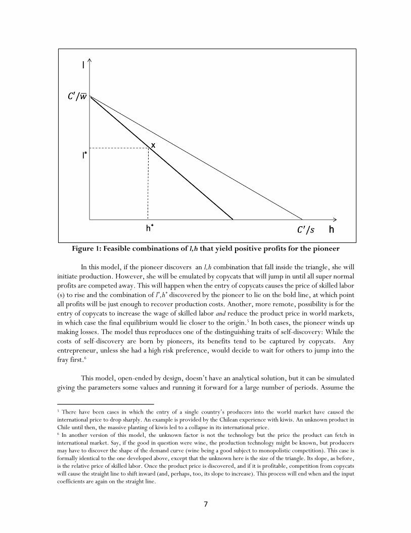
Equation (7) describes a straight line with – 𝑠/�̅� as its slope and intercepts 𝐶′/�̅� and 𝐶′/𝑠 in the vertical and horizontal axes respectively. Thus the area bounded by the axes and the hypotenuse of the triangle represent all the combinations of input coefficients that are profitable. All the combinations that lie on the straight line yield sufficient profits to recover investment costs (i.e., have zero rents).

7

Figure 1: Feasible combinations of l,h that yield positive profits for the pioneer

In this model, if the pioneer discovers an l,h combination that fall inside the triangle, she will initiate production. However, she will be emulated by copycats that will jump in until all super normal profits are competed away. This will happen when the entry of copycats causes the price of skilled labor (s) to rise and the combination of l*,h* discovered by the pioneer to lie on the bold line, at which point all profits will be just enough to recover production costs. Another, more remote, possibility is for the entry of copycats to increase the wage of skilled labor and reduce the product price in world markets, in which case the final equilibrium would lie closer to the origin.5 In both cases, the pioneer winds up making losses. The model thus reproduces one of the distinguishing traits of self-discovery: While the costs of self-discovery are born by pioneers, its benefits tend to be captured by copycats. Any entrepreneur, unless she had a high risk preference, would decide to wait for others to jump into the fray first.6 This model, open-ended by design, doesn’t have an analytical solution, but it can be simulated giving the parameters some values and running it forward for a large number of periods. Assume the

5 There have been cases in which the entry of a single country’s producers into the world market have caused the international price to drop sharply. An example is provided by the Chilean experience with kiwis. An unknown product in Chile until then, the massive planting of kiwis led to a collapse in its international price. 6 In another version of this model, the unknown factor is not the technology but the price the product can fetch in international market. Say, if the good in question were wine, the production technology might be known, but producers may have to discover the shape of the demand curve (wine being a good subject to monopolistic competition). This case is formally identical to the one developed above, except that the unknown here is the size of the triangle. Its slope, as before, is the relative price of skilled labor. Once the product price is discovered, and if it is profitable, competition from copycats will cause the straight line to shift inward (and, perhaps, too, its slope to increase). This process will end when and the input coefficients are again on the straight line.

8

planner’s objective function is to maximize growth through the introduction of modern sectors into the economy. The planner has a lower rate of time preference than the private entrepreneurs and are thus willing to subsidize, fully or in part, the investment in information gathering. The planner will also have to decide which infrastructure projects she will invest in. Finally, she can set tax rates on profits. Tax rates can be the same for the modern and traditional sectors, or they can be differentiated. In addition, in the modern sector the tax rate on pioneers can be different from the one that applies to copycats. As noted above, we assume that the government has no borrowing ability and that the public budget must balance. This setup makes for several interesting possibilities. In the first place, if taxes in the modern sector are set too high, it may not be profitable for pioneers to engage in search activities. Second, if the planner subsidizes search costs, she may not have sufficient resources left to build infrastructure. Third, low taxes may encourage search but they may not generate sufficient tax revenue to either subsidize search costs or new infrastructure projects. Finally, investment in skill-intensive production may put upward pressure on the skilled-labor wage, but only the emergence of skill-intensive output ensures the future growth in the availability of skilled labor.

III. The choices facing the planner

In this model, the planner has three policy levers. One is to choose the family of sectors for which she will provide infrastructure. Second, she can choose to subsidize part or all of search costs (in the model, C). Third, she can set the level and agents to which profit taxes will apply. The latter can be uniform for all sectors and types of agents. Alternatively, tax rates can be differentiated between pioneers and copycats within each sector, or between the traditional and the modern sector. To simplify, we will vary tax rates between pioneers and copycats and assume a fix tax rate on the traditional sector.

As regards the choice of infrastructure projects, we can distinguish two broad set of

possibilities. In the first one, the planner has no idea about the values of the input-output coefficients as between sectors. In this case, the infrastructure projects are chosen at random.

Alternatively, the planner can guess pretty accurately the expected mean level of the

coefficients of each family of sectors, but does not know their distribution by specific sector around that mean.

Therefore, the planner has to choose among the following set of alternatives of infrastructure

projects: 1. The easiest choice is to pick families of sectors at random. 2. Choose projects that serve families of sectors with the highest expected value of the labor

coefficient (highest E(l)). This would correspond to a choice based on comparative advantage.

3. Choose projects serving families of sectors with the highest E(h) and lowest E(l). Although somewhat counterintuitive, this choice would give pride of place to sectors with externalities in human capital formation.

4. Choose projects serving potential sectors with the lowest E(h), again on the basis of comparative advantage and for the sake of saving on the scarce factor.

9

As already noted, the planner must then decide to subsidize search costs (C) and what proportion of such costs, the values of the profit tax rates, and whether she will differentiate as between the traditional sector and pioneers and copycats in the modern sectors. The sequence of running the model is the following:

1. Start with initial values on subsidies and tax rates, traditional sector output, and the values

of the search investments (C’s); 2. The government then collects tax revenues and builds infrastructure; 3. Determine the sectors that emerge during the next period; 4. This generates supply and demand for skilled labor (H) in the next period, and determines

the wage for skilled labor (s); 5. The model is run for 50 periods ahead and one obtains a final output level and a final

accumulation of skilled labor; 6. The simulations are repeated for all possible combinations of a variety of choices of tax

rates and for two rates of information investment subsidy.

As can be seen in table 1, subsidizing search costs is a dominant strategy: no matter what the combination of tax rates used, the strategy with subsidy yields a larger final output and higher final skilled labor.

Table 1: Basic results of running the model for 50 periods

(growth rates per annum in percentage)

C subsidy

Strategy Growth rate of output

Growth rate of skilled labor

Tax on pioneers (%)

Tax on copycats (%)

NO

Random 1.5 1.6 0 50

Highest E(l) 1.0 1.4 0 50

Highest E(h), Lowest E(l) 1.6 1.6 0 50

Lowest E(h) 1.6 1.5 0 45

YES

Random 2.2 2.6 5 50

Highest E(l) 2.1 2.2 0 40

Highest E(h), lowest E(l) 2.5 2.6 5 50

Lowest E(h) 2.0 2.2 0 50

While the choice of subsidizing search costs is indeed the one that maximizes output over the period, the choice of infrastructure projects is much less of a determinant in final results. The rates of growth of output fluctuate about half of a percentage point depending on the choice of sector families made. In the absence of information with regard to the expected values of the input-output coefficients, the best choice for infrastructure would be a random one. Taxes don’t seem to deter copycats in the model. The optimal tax rate on copycats (that is, the one that maximizes growth) is 50 per cent of profits (which turns out to be equal to the rate assumed on traditional sector profits). On the other hand, the tax on pioneers should be kept low (5 per cent) if one wishes to maximize growth. In other words, the intuition is that, given the information externalities involved, the planner ought to subsidize the investment in information and, in addition, tax pioneers lightly, while recouping its investments on information and subsidies with high taxes on the traditional sector and on copycats.

10

In the following figures, I show some of the simulations that are behind the summary table 1. In all cases, subsidizing information costs leads to higher final output, so that I show only the graphs obtained under that assumption. The three-dimensional graphs show total output in the vertical axis and the tax rates on pioneers and copycats, respectively, on the horizontal axes.

Figure 2 Final output after 50 periods, with government subsidizing information and choosing

infrastructure projects that with highest E(h)/lowest E(l) jointly

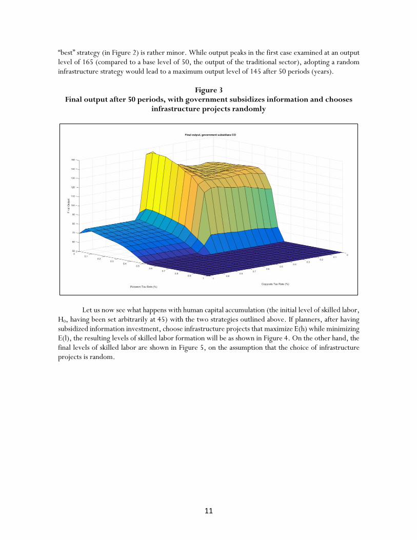
Figure 2 is built on the assumptions that the planner fully subsidizes information investment and chooses infrastructure projects that have meet the joint condition of having the highest expected value of the skilled-labor input coefficient and the lowest expected value of the unskilled labor coefficient. In this case, as the profit tax on pioneers rises above 5%, final output monotonically decreases and, at tax rates above 40%, it goes to zero, regardless of the profit tax on copycats. The latter, which is an important source of revenue to the government, shows interesting properties. If the rate on pioneers is above 50%, there is no output increase regardless of the tax rate on copycats. As the tax on pioneers falls, the economy’s total output increases together with the tax rate on copycats. The combination of tax rates that maximizes output is 5% for pioneers and 50% for copycats. Figure 3 is very similar, except that the selection of infrastructure projects is random. If one assumes, perhaps more realistically, that governments don’t know the input-output coefficients of different families of sectors – and not even their expected value – the strategy of randomly selecting infrastructure projects makes more sense.7 In fact, the loss in output from this strategy relative to the

7 Of course, one has to assume that the planner won’t choose projects where the country can’t hope to develop comparative advantage. For example, the planner is smart enough not to launch a policy such as Brazil’s information technology program in the 1980s, which had absolutely no positive results for the economy. See Crespi, Fernández-Arias, and Stein, 2014, pp. 16-18.

11

“best” strategy (in Figure 2) is rather minor. While output peaks in the first case examined at an output level of 165 (compared to a base level of 50, the output of the traditional sector), adopting a random infrastructure strategy would lead to a maximum output level of 145 after 50 periods (years).

Figure 3 Final output after 50 periods, with government subsidizes information and chooses

infrastructure projects randomly

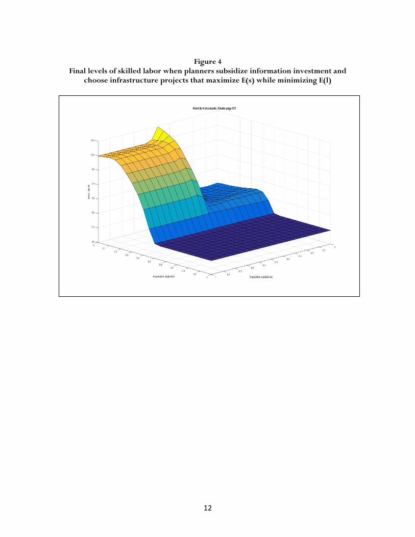
Let us now see what happens with human capital accumulation (the initial level of skilled labor, H0, having been set arbitrarily at 45) with the two strategies outlined above. If planners, after having subsidized information investment, choose infrastructure projects that maximize E(h) while minimizing E(l), the resulting levels of skilled labor formation will be as shown in Figure 4. On the other hand, the final levels of skilled labor are shown in Figure 5, on the assumption that the choice of infrastructure projects is random.

12

Figure 4

Final levels of skilled labor when planners subsidize information investment and choose infrastructure projects that maximize E(s) while minimizing E(l)

13

Figure 5

Final levels of skilled labor when planners subsidize information investment and choose infrastructure projects randomly

The results are quite similar than those for output. Human capital formation is maximized when taxes on pioneers are close to zero and taxes on copycats are in the 40-50% range.

IV. Changing some assumptions

We tried a large number of different assumptions on the percentage of information costs that is subsidized, subsidies on the hiring of skilled labor, and others. Here I report only those that are related to the introduction of a subsidy of 50% of information costs, rather than the full subsidy assumed in the first set of exercises. Why and under what circumstances should the planner withhold a full subsidy of information costs? In the first place, costs could be higher than assumed in the first set of simulations. We set information costs at 1.5, rather than at unity for this group of exercises. Second, full subsidies on information investments leave less resources for investments in infrastructure. Third, the planner may wish pioneers to have some “skin in the game”, for moral hazard reasons.

Then, here we assume that information costs are 50% higher than in the first group of

simulations and that the planner offers considers three sets of options: 0, 50% and 100% subsidies on information investment by pioneers. The results are shown in table 2.

14

Table 2: Results of running the model, assuming that information costs are 50% higher than those assumed in the first set of runs, and that the planner considers the option of

subsidizing 50% of information investments

C subsidy

Strategy Growth rate

of output Growth rate of

skilled labor Tax on

pioneers (%) Tax on

copycats (%)

0%

Random 1.5 1.6 0 50

Highest E(l) 1.0 1.4 0 25

Highest E(h), lowest E(l) 1.6 1.6 0 50

Lowest E(l) 1.7 2.7 0 50

50%

Random 2.2 2.6 0 50

Highest E(l) 1.9 1.9 0 25

Highest E(h), lowest E(l) 2.5 3.0 5 50

Lowest E(l) 2.3 2.6 0 50

100%

Random 2.1 2.6 0 50

Highest E(L) 2.1 2.2 0 40

Highest E(h), lowest E(l) 2.5 3.0 0 50

Lowest E(l) 2.3 1.2 0 50

As can be seen, the growth rate of the economy is about the same when the subsidy on

information investments is 50% of the total, when the planner chooses infrastructure projects that maximize the expected value of the skilled labor coefficient while minimizing the expected value of the labor coefficient, and when tax rates are 50% on copycats and zero on pioneers. The results don’t vary qualitatively from what we found in the first set of simulations. However, given the moral hazard incurred in subsidizing 100% of information investments (and not considered at all in these mechanical exercises), it is entirely reasonable that the planner will require a commitment from pioneers. The rationale for the same results being obtained with a 50% subsidy as with a 100% subsidy could be that the resources saved by the planner on subsidies leaves her with more room for further infrastructure investments.

The various combinations of tax rates for the options with a subsidy of 50% of the investment

in information and assuming a choice of infrastructure that maximizes the expected skilled-labor coefficient while minimizing the expected unskilled-labor coefficient are shown in figures 6 and 7. Figure 6 plots the final level of output for various choices of tax rates on pioneers and copycats, while figure 7 does the same for final levels of skilled labor.

15

Figure 6 Final output after 50 periods, with subsidy of 50% of information investment, with choice of infrastructure that maximizes E(h) and minimizes E(s)and under various

profit tax rates on pioneers and copycats

16

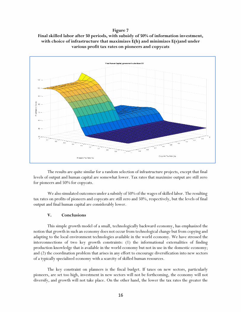
Figure 7 Final skilled labor after 50 periods, with subsidy of 50% of information investment,

with choice of infrastructure that maximizes E(h) and minimizes E(s)and under various profit tax rates on pioneers and copycats

The results are quite similar for a random selection of infrastructure projects, except that final levels of output and human capital are somewhat lower. Tax rates that maximize output are still zero for pioneers and 50% for copycats. We also simulated outcomes under a subsidy of 50% of the wages of skilled labor. The resulting tax rates on profits of pioneers and copycats are still zero and 50%, respectively, but the levels of final output and final human capital are considerably lower.

V. Conclusions

This simple growth model of a small, technologically backward economy, has emphasized the

notion that growth in such an economy does not occur from technological change but from copying and adapting to the local environment technologies available in the world economy. We have stressed the interconnections of two key growth constraints: (1) the informational externalities of finding production knowledge that is available in the world economy but not in use in the domestic economy; and (2) the coordination problem that arises in any effort to encourage diversification into new sectors of a typically specialized economy with a scarcity of skilled human resources.

The key constraint on planners is the fiscal budget. If taxes on new sectors, particularly

pioneers, are set too high, investment in new sectors will not be forthcoming, the economy will not diversify, and growth will not take place. On the other hand, the lower the tax rates the greater the

17

difficulty of planners in investing in infrastructure in subsequent periods. Such infrastructure is key to the emergence of new sectors and continued diversification.

We have seen that the dominant strategy is to subsidize investment in information leading to

the establishment of new sectors. There is no policy option without the subsidy that is better than any option with the subsidy. This is to be expected from the structure of the model, which emphasizes the incorporation into the economy of hitherto absent (and presumably higher-productivity) lines of production. The difference in growth rates of subsidizing the full costs of obtaining information and only 50% of such costs are more or less of the same order of magnitude. Given the moral hazard involved in full subsidization, it is probably wiser to opt for a partial subsidy.

There is another externality that is worth mentioning. Since the model assumes that skilled

labor is of the on-the-job-training type, demand from sectors that are skilled-labor-intensive has a positive spin-off on the economy. By construction, only new sectors demand skilled labor. Once labor is skilled, it is able to skill others. That is the reason that the best strategy for infrastructure selection involves choosing projects that serve skill-intensive families of sectors.

Clearly, this type of model is highly unrealistic. But so are one-sector models, which obscure

just as much as they illuminate. I hope that it will encourage others to build models that reflect the basic stylized facts of economic growth in a poor economy: the importance of copying existing technologies and the constraints that process faces.

18

Appendix: Initial values of the main variables, coefficients, and simulation procedure Initial values and coefficients C = 1 and 1.5, the latter when the simulation allows for a 50% subsidy of information investment; the

values of search costs are equal for all sectors

𝜆 = 75, equal for all projects pij = 1.4 times the price of the good in the traditional sector; equal for all new sectors YT = 50 (units of output, and value, of the traditional sector output, held constant)

T = 0.50 (for all runs of the model) H0 = 25 (initial levels of human capital)

𝜇 = 0.25 (increase in human capital per period) r = 0.10 (discount rate)

𝛽 =1

1+𝑟 (impatience factor of pioneers)

= 1/1.10 = 0.90, when the planner subsidizes partly or wholly information investment, and = 1/1.17 = 0.85, when there are no subsidies on information investment The model was programmed in Matlab following a certain sequence: During the first stage the aggregate output of the economy is calculated, and the skilled-labor wage is determined endogenously. Remember that in the first period only the traditional sector exists. Demand for unskilled and skilled labor in the modern sector is determined with a random uniform function. The

supply of skilled labor in period one is determined by equation 𝐻1 = (1 + 𝜇)𝐻0. In the second stage, the planner collects tax revenues from the traditional sector (and in later periods, from those modern sectors that arise). The calculations also allow for transferring to the period t+1 whatever tax revenue is left over from period t. In the third stage, the planner determines the infrastructure projects to be built. This is essential to the workings of the dynamic model, because subsectors can arise only if they belong to the general family of sectors for which the infrastructure is built. These two latter stages determine the variables in the following period. The full model is run for 50 periods. Growth rates are estimated for Y and H in the tables of results. The surfaces shown in figures 2 through 7 are expressed in final outputs and human capital relative to their initial values. In greater detail, the code is built with the following logic:

We first define a random function using a “twister”, which we use every time we create a normalized variable such as the levels of h and l for each sector. These take values in the continuum of zero to unity.

We also fix the number of repetitions of the model at 50 and take averages of the values of each variable.

19

We create the matrices that store the levels of aggregate output Y, H, the number of firms, the salary of skilled labor s, and the quantity of infrastructure projects built per period, for each of the 50 repetitions, for each possible combination of tax rates for pioneers and copycats. These are stored in 21x21 matrices.

We assume that there are 10 families of sectors and 10 sectors in each family; the parameters h and l are created as normalized variables derived from the random uniform functions.

Since we need to obtain the outputs of interest for each combination of tax rates that can be applied to pioneers and copycats, two rounds of iterations are nested, with the objective of filling in each ordered pair of the result matrices (containing Y, H, s, and l). This network of iterations contains 21 potential tax rates for pioneers and copycats per round, which is equivalent to testing the results of applying tax rate combinations by increasing them by 5 percentage points at a time.

Then we estimate the vectors indicating the coefficients h,l per unit of output required by each sector (and each family of sectors) in each repetition.

In the following step, we build the equations by which the planner orders families of sectors according to her infrastructure strategy. The planner has an idea of the expected values of the input coefficients of families of sectors, but she does not have the full information of those values for each sector within each family. She ranks the sectors according to the size of the h and l coefficients. In most cases, the optimal result is obtained when the planner maximizes the expected value of h (the skilled-labor coefficient per unit of output) while at the same time minimizing the expected value of l (the unskilled-labor coefficient per unit of output).

Vectors are created for each combination of tax rates that store the aggregate value of output and outputs of each sector and family of sectors. Other vectors that are created for each tax rate combinations are: (1) the government budget for infrastructure and subsidies to information investment; (2) firm profits; (3) the values of s that firms are willing to pay.

The quantity demanded of H and the skilled-wage salary (s) are jointly determined by ordering firms according to their willingness to pay, until all available supply of H is exhausted (market clearing assumption). Willingness to pay is determined by the following equation:

𝑠𝑖𝑗 =(𝑝𝑖𝑗−�̅�𝑙𝑖𝑗)

ℎ𝑖𝑗 (remembering that all Gi,j are set equal to 1). The supply of H is distributed to

the firms that make the cut and the model determines the family of sectors and, within them, the sectors that are active.

Each pioneer produces one unit of output. For every pioneer there are 10 copycats, also

producing one unit each. The output of pioneers is added to that of copycats, and to this the output

of the traditional sector (50) is added to obtain aggregate output.

The planner collects taxes on the basis of profits made by the three types of producers.

After deciding whether she will subsidize part or all of the costs of information investments,

the planner allocates her remaining budget to infrastructure projects, ranked according to various

sets of criteria (see text).

In the next round, the available H is brought up to date by adding up the H created in each

sector.

The planner needs to know whether the firms will be profitable during the next period. This

will depend on whether she has been willing to subsidize (fully or partially) the cost of information

investment.

20

The matrices mentioned above are filled and the planner determines which combination of tax

rates on pioneers and copycats result in the largest output after 50 periods.

References Agosin, M. R. (2009), “Export Diversification and Growth in Emerging Economies”, CEPAL Review 97: 115-131. Crespi, G., E. Fernández-Arias, and E. Stein, editors (2014), Rethinking Productive Development: Sound Policies and Institutions for Economic Transformation, Inter-American Development Bank, Washington, D.C. Gerschenkron, A (1962), Economic Backwardness in Historical Perspective, Harvard University Press, Cambridge, MA. Gollin, D. (2014), “The Lewis Model: A 60-Year Retrospective”, Journal of Economic Perspectives 28: 71-88. Hausmann, R. and D. Rodrik (2003), “Economic Development as Self-Discovery”, Journal of Development Economics 72: 603-633. Hausmann, R., J. Hwang, and D. Rodrik (2006), “What You Export Matters,” Working Paper, Center for International Development, Harvard University. Hausmann, R., and B. Klinger (2006), “Structural Transformation and Patterns of Comparative Advantage in the Product Space,” Working Paper No. 128, Center for International Development, Harvard University. Hesse, E. “Export Diversification and Economic Growth”, Commission on Growth and Development Working Paper No.21, World Bank, Washington, D.C., 2009. Imbs, J. and R. Wacziarg (2003), “Stages of Diversification”, American Economic Review 93: 63-86. Lewis, W. A. (1954), “Economic Development with Unlimited Supplies of Labour”, Manchester School, May: 400-449. Lucas Jr., R. E. (1993), “Making a Miracle”, Econometrica Vol. 61: 251-72. Murphy, K., A. Schleifer, and R. Vishny (1989), “Industrialization and the Big Push”, Journal of Political Economy 97: 1003-1026. Rosenstein-Rodan, P. N. (1943), “Problems of Industrialization of Eastern and South-Eastern Europe”, The Economic Journal 53: 202-211.