A Model of Airline Pricing: Capacity Constraints and · PDF file41 A Model of Airline Pricing: Capacity Constraints and Deadlines to departure, prices start rising. Instead of monotonically

Journal of Quantitative Economics, Vol. 5, No. 2, 2007 40

A Model of Airline Pricing: CapacityConstraints and Deadlines

Shubhro Sarkar∗†

Abstract

We study monopolistic pricing, with a capacity constraint, of a good thatloses its value after three periods. In each period a continuum of buyers, eachof whom might be one of two types, enter. Each of the buyers chooses eitherto make a purchase as soon as they enter, or to wait for a lower price. Theprice path is found to be strictly non-decreasing, u-shaped or horizontal fordifferent proportions of buyers with a higher willingness to pay. Any strategyinvolving ‘final sales’ is non-optimal. The predictions are empirically tested.

Keywords: Dynamic pricing, capacity constraints, time-sensitive goods, subgameperfection.JEL codes: L10, L93, C72.

1 IntroductionIt is a well-known fact that passengers on the same flight, traveling in the same class,often end up paying different prices for their tickets. This is because the prices ofsuch tickets vary over time, often within the span of a few hours. While buyershave the option of purchasing tickets months prior to the date of departure, casualobservation suggests that the prices offered by an airline are high if a purchase isattempted too early, drop after a period of time and then prior to departure theyrise again. An empirical study by Stavins (2001) indicates that five weeks prior

∗Indira Gandhi Institute of Development Research, Mumbai, 400065, India. Email:[email protected]

†I would like to thank Kalyan Chatterjee, Tomas Sjostrom, Mark Roberts, Susanna Esteban, JunXue, Alejandro Riano, Luis Martins and Sreya Kolay for several helpful suggestions and comments.I would also like to thank Sergio DeSouza for helping me write a program in order to verify theresults.

41 A Model of Airline Pricing: Capacity Constraints and Deadlines

to departure, prices start rising. Instead of monotonically reducing prices, sellingevery available seat and waiting for takeoff, the airline instead, chooses to save acertain number of seats for future buyers, who would be willing to pay a high pricefor the same seats. This shows, that in order to solve for the optimal price path ofsuch goods, we need a model with a finite time horizon, where one or many sellerswhile facing a capacity constraint, offer(s) a finite measure of units for sale. In eachperiod, a continuum of buyers, each of whom might be one of two types, enters themarket. The seller chooses, without precommitment, price and measure of units tooffer in each period, while each of the buyers choose either to make a purchase assoon as they enter, or to wait for a lower price which might be made available in thefuture.

The operations research literature identifies airline ticket pricing as dynamicpricing (also known as yield management), where the product ceases to exist ata certain point in time and capacity can only be added at a very high marginalcost. The product being discussed here is non-durable, non-storable and cannot beresold. We could consider an airline ticket to be a futures contract on a service tobe provided by the airline in the future. As the airline attempts to sell tickets overtime, it is in effect “signing” contracts with different customers on different terms.As the seller is unable to precommit to the terms of the contract in the future and isin effect competing against future versions of himself (herself), he (she) faces thesame intertemporal and time-consistency problems as a durable-goods monopolist.Other examples of such products include hotel rooms, generated electricity or other“sell before”goods where transactions occur through a futures contract (McAfee& Velde). Given the similarities in the problems facing an agent signing multiplefutures contracts (airline) and a durable goods monopolist, we can refer to the vastliterature on time-consistency issues in a durable-goods monopoly.

In this paper, we use a model which extends that of a durable-goods monopolymodel by Conlisk, Gerstner and Sobel (CGS, 1984). In their infinite time horizonmodel, a new cohort of consumers enters the market in each period. The consumersin each group differ amongst themselves in terms of the valuation for the good.Some of these buyers choose to make a purchase in the same period, while othersdecide to wait for a lower price. Usually the single seller, who does not face anycapacity constraint, prefers to sell the product at a price just low enough to sellimmediately to consumers with a high willingness to pay, as long as revenue earnedfrom selling to “high” type buyers exceeds revenue earned from selling to “low”type buyers. However, as sufficient number of consumers with a lower willingnessto pay accumulate in the market, the seller holds a ‘sale’ by dropping the price lowenough, so that buyers with lower willingness to pay can buy the product. Thisleads to an equilibrium where periodic ‘sales’ are held and the corresponding pricepath is cyclic. We extend this model, by introducing a capacity constraint for the


single seller and by solving for the equilibrium for a finite time horizon.The main predictions of the theoretical model are as follows. First, a sufficiently

patient seller never offers any ‘sale’ in the last period. This is because the sellerchooses to reserve some units for sale in the last period and offer them at highprices to high valuation buyers who enter the market in that period. Second, themeasure of units offered for sale in any period where the seller chooses to offer thegood to both types of buyers is a decreasing function of the proportion of high typebuyers in the market. Third, the shape of the price path is horizontal, u-shaped orstrictly non-decreasing for various ranges of parameter values. For example, forroutes with the highest proportion of high type buyers, sellers had no incentive tooffer a sale and the price path is horizontal. Routes with lower proportions of hightype buyers have price paths which are strictly non-decreasing or u-shaped.

We collected data on prices over 15 weeks for 30 routes in the US. While thefirst prediction was found to be empirically valid, we find little evidence to supportthe hypothesis that the price path should be horizontal for routes with the highestproportion of buyers with a higher willingness to pay. We classified the routes intolow, medium and high proportion of high type buyers and find that prices increase asthe date of departure grows closer for all three types of routes. The rate of increasewas highest for routes with the highest fraction of high type buyers. We did findsome evidence for a u-shaped price path for routes with low or medium proportionof high type buyers when we looked at the last 10 weeks of observations.

2 Review of LiteratureAs mentioned in the previous section, even though airline tickets are not durable,the intertemporal problems facing a seller of airline tickets are identical to thosefacing a durable goods monopolist. We thus begin the review of literature section byreferring to the literature on durable goods monopoly. The problem of intertemporalprice discrimination as faced by a durable-goods monopolist has been the focusof several papers over the years. In his seminal paper, Coase (1972) conjecturedthat a durable-goods monopolist would be unable to exert any monopoly power.This is because rational buyers would anticipate correctly that in the absence ofprecommitment to future prices, the monopolist would reduce prices in an attemptto cater to residual demand and would refuse to buy the product as long as pricesremained above the competitive level.

There are two assumptions, which are crucial to our model. The first is thatthe seller faces a capacity constraint, while the second is the constant influx ofnew buyers. It has been found that the Coase conjecture fails to hold under theseassumptions. McAfee and Wiseman (2003) show that capacity costs of arbitrarily


small degree can eliminate the zero profit conclusion. Capacity costs borne by theseller serve as a strong commitment device, as the choice of capacity enables theseller to slow the sales, reduce the fall in prices and thus permits the seller to setinitial prices above marginal costs. Papers by Sobel (1984), Conlisk, Gerstner andSobel (1984) show that the equilibrium in a model with a continual influx of newbuyers involves price cycles where each seller produces a homogeneous good andsells it to consumers with different willingness to pay. A cyclic price path is alsoobtained in a paper by Narasimhan (1989), who uses a framework similar to thatof CGS but assumes that the entry of new consumers is governed by a diffusionprocess. In his model, the number of buyers who enter the market in each period isa function of cumulative sales and is time variant. Unlike Conlisk et al. the marketsize in his model is fixed, such that after some time saturation effects set in.

An alternate outlook is presented in papers by Brumelle and McGill (1993)and Wollmer (1992), who solve for an optimum airline seat booking policy, wherelower fare class customers book tickets before higher fare class passengers. Inthese papers, airlines solve for a critical number of seats in each fare class, whichare reserved for potential future passengers who are willing to pay a higher price.Booking requests for a particular fare class are accepted if and only if the number ofempty seats is strictly greater than its critical level and rejected otherwise. Wollmershows that this critical value is a decreasing function of the fare price and is equalto zero for the highest fare (class). However, these papers lack the flavor of durablegoods, as buyers do not have the option of staying in the market to wait for a lowerprice, while sellers do not compete with future incarnations of themselves.

Stavins (2001) addresses the issue of how airline prices move over time in apaper in which she examines how price discrimination changes with market con-centration in the airline market. Price discrimination is found to increase as themarkets become more competitive. The data set included fares offered 35 daysprior to departure, followed by 21 days prior to departure, 14 days prior to depar-ture and finally 2 days prior to departure. The data thus allowed for examinationof how prices change as the departure date drew closer. From the OLS regressionit was discovered that cheaper fares disappear, leaving only more expensive ticketsfor sale.

McAfee and Velde (2004) provide an extensive survey of yield management re-search in operations research journals and then test the predictions of these modelswith airline pricing data collected from 1,260 flights. They test the following fivepropositions. First, prices fall as the date of departure approaches. Second, pricesrise initially. Third, competition reduces the variance in prices. Fourth, priceschange as the number of empty seats remaining change and finally fifth, prices offlights leaving from substitute airports or departing at substitute times are corre-lated. They find that prices increased $50 in the week before takeoff on top of a rise


of $28.20 the previous week. Thus the first proposition was empirically false andtheories which assume that customers arriving in the market at different points intime are identical are invalid. Overall, there was scant empirical evidence in favorof the major theoretical predictions. 1 However, the routes considered by them hadmultiple airlines serving them, such that their results are inapplicable for modelswith a single seller.

Etzioni et al (2003) devise an algorithm called Hamlet, which when trained ona data set comprising of over 12,000 observations over a 41 day period, was ableto generate a predictive model which enabled 607 simulated passengers an averagesavings of 27%. Flights were found to have discernible price tiers and the numberof such tiers varied from two to four, depending on the airline and the particularflight. They find that pricing policies tend to be similar for airlines belonging to thesame category and that the prices fluctuate more and are more expensive for biggerairlines. Finally, they observe that prices increase two weeks prior to departurewhich corroborates the empirical finding of Stavins.

The main contribution of this paper is to provide insights into the relationshipbetween the proportion of buyers with a higher willingness to pay and the corre-sponding shape of the price path, from a model which incorporates some essentialfeatures of an airline pricing problem. The paper proceeds as follows. In the follow-ing section a basic three-period model is developed and strategies for both playersoutlined. Section 4 identifies possible candidates for subgame perfect outcomesand describes conditions under which we get the different price paths. Section 5describes the data, 6 the empirical model while section 7 presents the results. Sec-tion 8 contains the conclusions.

3 Model

Setting. Time is discrete. We can consider a finite horizon model of T periods. Thegood has a lifetime of T periods, after which it is assumed to be lost forever. Inorder to consider a simple version, we assume that T = 3.

Supply side. There is a single seller of the product. The monopolist faces con-stant marginal cost, assumed without loss of generality to be zero. The total measureof units of the product (seats) available to the monopolist is 3. The seller chooses tooffer a continuum of units of measure qi ∈ [0,3] for i = 1,2,3 in period i. The selleralso chooses price pi for period i, so as to maximize sum of discounted revenueearned, calculated at discount factor ρ, with 0 < ρ < 1. The monopolist cannot rentthe product; at any given date, the monopolist cannot make binding commitments

1They do not specify as to whether the second proposition was found to be empirically valid.


about future prices and measure of units to be offered for sale.Demand side. A continuum of buyers of measure 2 enter the market in each

period, with each buyer having unit demand. Buyers in each cohort can be one oftwo types. A continuum of buyers of measure 2α (with 0 < α < 1) enter the marketin each period and have valuation for the product given by V1, while a continuumof buyers of measure 2(1−α) enter the market in each period and value the goodat V2, where V1 > V2 > 0. Buyers with valuation V1 are said to be of ‘high’ type,while buyers with valuation at V2 are said to be of ‘low’ type. We assume that themajority of buyers entering the market in each period are of low type and henceα ∈ (0,1/2).

Buyers are rational. Each buyer on entering the market decides either to pur-chase the product in the current period or to wait for a lower price, except for buyersin the last period, who either decide to buy or not to buy the product in the last pe-riod. In the event that the buyer is indifferent between buying in the current periodand waiting (or not to buy), the buyer is assumed to make the purchase immediately.Buyers assume that their own decision as to when to buy the product has no bearingon other buyer’s decision as to whether and when to buy the same product. This isa consequence of the assumption that we have a continuum of buyers in the market.The probability that the buyer will get the product in period i is given by Φi which isdetermined endogenously. Once a consumer buys the product, he or she leaves themarket forever. A consumer who has not bought the product stays in the market tillperiod 3, regardless of when he or she first entered the market. Finally, no resalesare allowed. All consumers are price takers, and they have no bargaining power.This, once again, is a consequence of the assumption that we have a continuum ofbuyers in the market.

Timing of events. At the beginning of period 1, the seller announces the price forthe first period, p1 and the measure of units available for purchase, q1. A continuumof buyers of measure 2 enter the market in the first period, of which buyers ofmeasure 2α are of ‘high’ type and buyers of measure 2(1−α) are of ‘low’ type.Each buyer decides whether to buy the product in the first period, or to wait for alower price which might be made available in the future. Based on p1 and q1, theseller knows the measure of units that were actually sold in the first period. At thebeginning of the second period, the seller announces price for period 2, p2 and themeasure of units available for sale in the second period, q2. A new cohort of buyers(of measure 2) enter the market in the second period. These buyers along with thebuyers who decided not to buy the product in period 1 and hence chose to remainin the market then constitute the total measure of buyers in the market in the secondperiod. Each of these buyers in turn decide either to purchase the product at pricep2 or to wait for a lower price in period 3. A similar sequence of events follow inperiod 3, except for the fact that buyers of both types in period 3, choose either to


purchase or not to purchase the good in the last period.We assume that the type of each buyer is publicly observable, such that we

have a complete information model. We further assume that, even though the sellerknows the type of each and every ‘active’ buyer in the market at any point of time, heor she is unable to price discriminate and must charge (or announce) a single pricein every period.2 We solve for the subgame perfect outcomes of the game describedabove for various combinations of parameter values. Conversely, we could haveassumed that the buyers’ types are not observable. In that case, Perfect Bayesianequilibrium would have been the appropriate equilibrium concept, where we wouldhave to explicitly specify how agents form beliefs for information sets on and offthe equilibrium path.

Notation. The following notation is introduced in order to describe the totalmeasure of ‘high’ and ‘low’ type buyers in the market at each point of time, as wellas the measure of units left with the seller at the beginning of each period.

bHi = Total measure of ‘high’ type buyers in the market including ones entering

the market in period i.bL

i = Total measure of ‘low’ type buyers in the market including ones enteringthe market in period i.

si = Measure of units left with the seller at the beginning of period which is afunction of pi−1,qi−1,bH

i−1,bLi−1 and si−1, where pi−1,qi−1 are control variables and

bHi−1,b

Li−1,si−1 are state variables for period i−1.

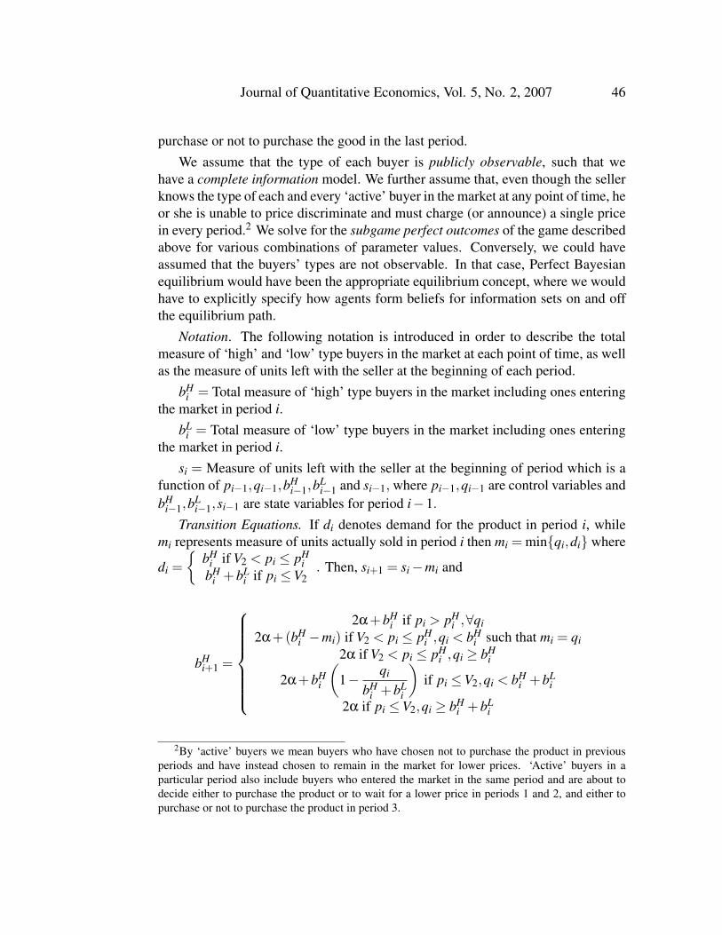
Transition Equations. If di denotes demand for the product in period i, whilemi represents measure of units actually sold in period i then mi = min{qi,di} where

di ={

bHi if V2 < pi ≤ pH

ibH

i +bLi if pi ≤V2

. Then, si+1 = si−mi and

bHi+1 =

2α+bHi if pi > pH

i ,∀qi2α+(bH

i −mi) if V2 < pi ≤ pHi ,qi < bH

i such that mi = qi2α if V2 < pi ≤ pH

i ,qi ≥ bHi

2α+bHi

(1− qi

bHi +bL

i

)if pi ≤V2,qi < bH

i +bLi

2α if pi ≤V2,qi ≥ bHi +bL

i

2By ‘active’ buyers we mean buyers who have chosen not to purchase the product in previousperiods and have instead chosen to remain in the market for lower prices. ‘Active’ buyers in aparticular period also include buyers who entered the market in the same period and are about todecide either to purchase the product or to wait for a lower price in periods 1 and 2, and either topurchase or not to purchase the product in period 3.


bLi+1 =

2(1−α) if pi ≤V2,qi ≥ bH

i +bLi

2(1−α)+bLi

(1− qi

bHi +bL

i

)if pi ≤V2,qi < bH

i +bLi

2(1−α)+bLi if pi > V2,∀qi

where pHi is the price in period i which makes ‘high’ type buyers indifferent be-

tween buying the product in period i and waiting for a lower price in period i+1.A strategy for the monopolist specifies for each period, price and measure of

units to be offered to the buyers as a function of the history of the game. A strategyfor the buyer of each type on the other hand, specifies at each time and after eachhistory (in which he or she has not previously purchased or in case he or she has justentered the market) whether to accept or to reject the monopolist’s offered price.

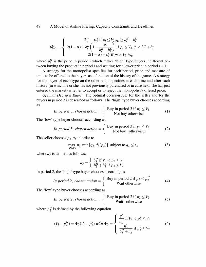
Optimal Decision Rules. The optimal decision rule for the seller and for thebuyers in period 3 is described as follows. The ‘high’ type buyer chooses accordingas

In period 3, chosen action ={

Buy in period 3 if p3 ≤V1Not buy otherwise (1)

The ‘low’ type buyer chooses according as,


Buy in period 3 if p3 ≤V2Not buy otherwise (2)

The seller chooses p3,q3 in order to

maxp3,q3

p3.min{q3,d3(p3)} subject to q3 ≤ s3 (3)

where d3 is defined as follows:

d3 ={

bH3 if V2 < p3 ≤V1

bH3 +bL

3 if p3 ≤V2

In period 2, the ‘high’ type buyer chooses according as


Buy in period 2 if p2 ≤ pH2

Wait otherwise (4)



Buy in period 2 if p2 ≤V2Wait otherwise (5)

where pH2 is defined by the following equation

(V1− pH2 ) = Φ3(V1− p∗3) with Φ3 =

q∗3bH

3if V2 < p∗3 ≤V1

q∗3bH

3 +bL3

if p∗3 ≤V2

(6)


Here, we use a fixed-point argument. In period 2, the ‘high’ type buyers knowbH

2 ,bL2 . For the time being they fix the pH

2 of all other ‘high’ type buyers and calcu-late the corresponding bH

3 and bL3 . Given bH

3 ,bL3 these buyers can calculate the price

and measure of units the seller will offer in period 3, p∗3 and q∗3. Using p∗3, q∗3 andequation (6) these buyers are able to recover a pH

2 which should be equal to the oneoriginally assumed. pH

2 is thus the price the seller can charge in order to make the‘high’ type buyers indifferent between buying in period 2 and waiting for a lowerprice in period 3. At the beginning of period 2, the seller announces p2 and q2 inorder to

maxp2,q2

p2.min{q2,d2(p2)}+ρW (bH3 ,bL

3 ,s3) subject to q2 ≤ s2 (7)

where W is the continuation payoff earned by the seller in period 3 and d2 is definedas

d2 ={

bH2 if V2 < p2 ≤ pH

2bH

2 +bL2 if p2 ≤V2

Finally, we describe the optimal decision rules for the seller and the buyers forperiod 1. The ‘high’ type buyer chooses according as


Buy in period 1 if p1 ≤ pH1

Wait otherwise (8)



Buy in period 1 if p1 ≤V2Wait otherwise (9)

where pH1 is defined by the following equation

(V1− pH1 ) = Φ2(V1− p∗2) with Φ2 =

q∗2bH

2if V2 < p∗2 ≤ pH∗

2

q∗2bH

2 +bL2

if p∗2 ≤V2

(10)

At the beginning of period 1, the seller announces p1 and q1 in order to

maxp1,q1

p1.min{q1,d1(p1)}+ρW (bH2 ,bL

2 ,s2) subject to q1 ≤ 3 (11)

where W is the continuation payoff earned by the seller in period 2 and d1 is definedas

d1 ={

bH1 if V2 < p1 ≤ pH

1bH

1 +bL1 if p1 ≤V2


A subgame perfect Nash Equilibrium (SPNE) of this game will thus consist of astrategy profile, σ = (S,B) where S specifies a strategy on the part of the sellerwhich satisfies equations (3), (7) and (11) while B specifies strategies on the partof each buyer who decides either to buy or to wait for a lower price in periods 1and 2, and either to buy or not to buy in period 3, which satisfies equations (1), (4),(8) for ‘high’ type buyers and equations (2), (5) and (9) for ‘low’ type buyers. Theequilibrium is a symmetric equilibrium in the sense that in equilibrium all buyersof the same type, choose the same action in each period. With non-atomic buyers,unilateral deviations made by them affect neither the actions of other buyers orthose of the monopolist. Thus, in order to check for subgame perfection, onlyunilateral deviations by the seller are considered. If the seller deviates, the playerskeep following the optimal rules described above from that point of time onwards.This means if a player discovers a history of the game at any stage, which is notconsistent with the one expected in equilibrium, the player continues to follow hisor her optimal decision rule from that time onwards.

As the seller announces pi and qi at the beginning of each period i, we definea pricing policy (p1, p2, p3,q1,q2,q3) which describes the prices charged and theunits offered for sale in each period. It is possible to derive eight such possibleprice paths, where in each period, the seller decides either to sell only to ‘high’ typebuyers or to sell to both ‘high’ and ‘low’ types.

4 Candidates for Subgame Perfect Outcome

In this section, we examine the different possible pricing policies and the associatedprice paths from which the seller might choose, under different combinations of theparameters V1,V2,α and ρ. Since we are interested in decisions made by a patientseller, we further assume that ρ→ 1.

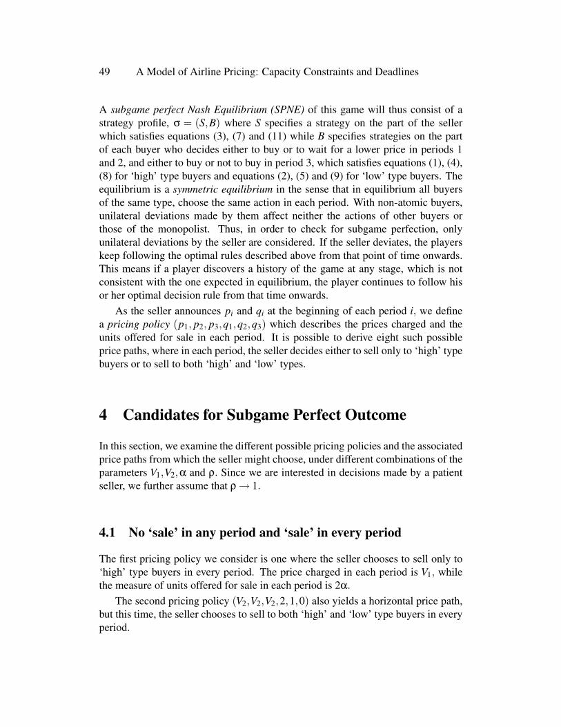
4.1 No ‘sale’ in any period and ‘sale’ in every period

The first pricing policy we consider is one where the seller chooses to sell only to‘high’ type buyers in every period. The price charged in each period is V1, whilethe measure of units offered for sale in each period is 2α.

The second pricing policy (V2,V2,V2,2,1,0) also yields a horizontal price path,but this time, the seller chooses to sell to both ‘high’ and ‘low’ type buyers in everyperiod.


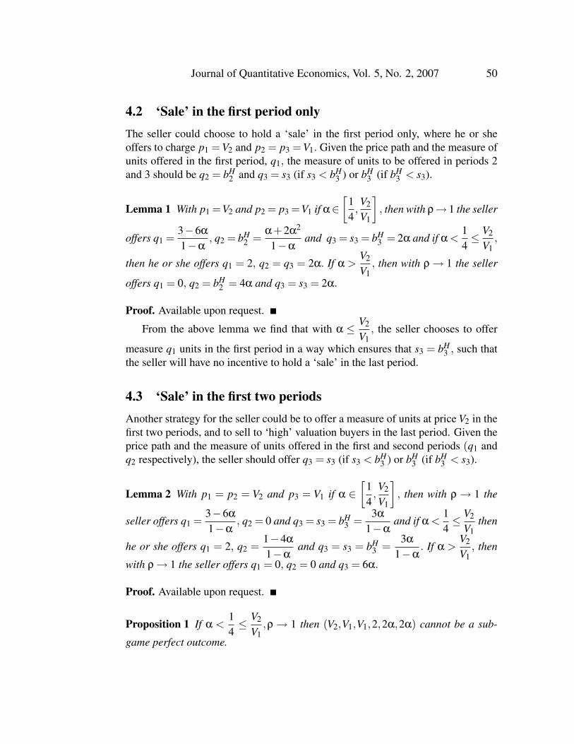
4.2 ‘Sale’ in the first period onlyThe seller could choose to hold a ‘sale’ in the first period only, where he or sheoffers to charge p1 = V2 and p2 = p3 = V1. Given the price path and the measure ofunits offered in the first period, q1, the measure of units to be offered in periods 2and 3 should be q2 = bH

2 and q3 = s3 (if s3 < bH3 ) or bH

3 (if bH3 < s3).

Lemma 1 With p1 =V2 and p2 = p3 =V1 if α∈[

14,V2

V1

], then with ρ→ 1 the seller

offers q1 =3−6α

1−α, q2 = bH

2 =α+2α2

1−αand q3 = s3 = bH

3 = 2α and if α <14≤ V2

V1,

then he or she offers q1 = 2, q2 = q3 = 2α. If α >V2

V1, then with ρ → 1 the seller

offers q1 = 0, q2 = bH2 = 4α and q3 = s3 = 2α.

Proof. Available upon request.

From the above lemma we find that with α ≤ V2

V1, the seller chooses to offer

measure q1 units in the first period in a way which ensures that s3 = bH3 , such that

the seller will have no incentive to hold a ‘sale’ in the last period.

4.3 ‘Sale’ in the first two periodsAnother strategy for the seller could be to offer a measure of units at price V2 in thefirst two periods, and to sell to ‘high’ valuation buyers in the last period. Given theprice path and the measure of units offered in the first and second periods (q1 andq2 respectively), the seller should offer q3 = s3 (if s3 < bH

3 ) or bH3 (if bH

3 < s3).

Lemma 2 With p1 = p2 = V2 and p3 = V1 if α ∈[

14,V2

V1

], then with ρ → 1 the

seller offers q1 =3−6α

1−α, q2 = 0 and q3 = s3 = bH

3 =3α

1−αand if α <

14≤ V2

V1then

he or she offers q1 = 2, q2 =1−4α

1−αand q3 = s3 = bH

3 =3α

1−α. If α >

V2

V1, then

with ρ→ 1 the seller offers q1 = 0, q2 = 0 and q3 = 6α.


Proposition 1 If α <14≤ V2

V1,ρ → 1 then (V2,V1,V1,2,2α,2α) cannot be a sub-

game perfect outcome.



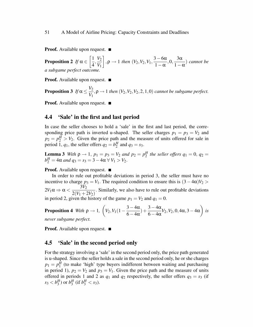
Proposition 2 If α ∈[

14,V2

V1

],ρ → 1 then (V2,V2,V1,

3−6α

1−α,0,

3α

1−α) cannot be

a subgame perfect outcome.


Proposition 3 If α≤ V2

V1,ρ→ 1 then (V2,V2,V2,2,1,0) cannot be subgame perfect.


4.4 ‘Sale’ in the first and last periodIn case the seller chooses to hold a ‘sale’ in the first and last period, the corre-sponding price path is inverted u-shaped. The seller charges p1 = p3 = V2 andp2 = pH

2 > V2. Given the price path and the measure of units offered for sale inperiod 1, q1, the seller offers q2 = bH

2 and q3 = s3.

Lemma 3 With ρ → 1, p1 = p3 = V2 and p2 = pH2 the seller offers q1 = 0, q2 =

bH2 = 4α and q3 = s3 = 3−4α ∀ V1 > V2.

Proof. Available upon request.In order to rule out profitable deviations in period 3, the seller must have no

incentive to charge p3 = V1. The required condition to ensure this is (3−4α)V2 >

2V1α⇒ α <3V2

2(V1 +2V2). Similarly, we also have to rule out profitable deviations

in period 2, given the history of the game p1 = V2 and q1 = 0.

Proposition 4 With ρ → 1,(

V2,V1(1−3−4α

6−4α)+

3−4α

6−4αV2,V2,0,4α,3−4α

)is

never subgame perfect.


4.5 ‘Sale’ in the second period onlyFor the strategy involving a ‘sale’ in the second period only, the price path generatedis u-shaped. Since the seller holds a sale in the second period only, he or she chargesp1 = pH

1 (to make ‘high’ type buyers indifferent between waiting and purchasingin period 1), p2 = V2 and p3 = V1. Given the price path and the measure of unitsoffered in periods 1 and 2 as q1 and q2 respectively, the seller offers q3 = s3 (ifs3 < bH

3 ) or bH3 (if bH

3 < s3).


Lemma 4 With p1 = pH1 , p2 = V2 and p3 = V1 if α≤ 2V2

V1 +V2, then with ρ→ 1 the

seller offers q1 = 2α, q2 =6α2−15α+6

2(1−α)and q3 = s3 = bH

3 =5α−2α2

2(1−α). On the

other hand, if α >2V2

V1 +V2, then with ρ → 1 the seller offers q1 = 2α, q2 = 0 and

q3 = 4α.

Proof. Available upon request.As was the case with strategies involving ‘sales’ in the first period only or the

first two periods, the seller offers measure q1 and q2 units in the first and second

period in a way which ensures that if α≤ 2V2

V1 +V2and ρ→ 1, s3 = bH

3 such that there

is no incentive for the seller to hold a ‘sale’ in the last period. With α >2V2

V1 +V2the

seller chooses to offer measure zero units for ‘sale’ in the second period.


14,V2

V1

], then with ρ→ 1

[V1(1−

6α2−15α+62(1−α)(4−2α)

)+

6α2−15α+62(1−α)(4−2α)

V2,V2,V1,2α,6α2−15α+6

2(1−α),5α−2α2

2(1−α)

]cannot be subgame per-

fect.


4.6 ‘Sale’ in the last two periodsFor strategies involving ‘sales’ in the last two periods, the seller charges p1 =pH

1 , p2 = p3 = V2 and offers q1 = 2α,q2 = 3− 2α,q3 = 0. These are the only qiswhich are time consistent.


V1<

2V2

V1 +V2and ρ→ 1 then

[V1

(1− 3−2α

4−2α

)+

3−2α

4−2αV2,

V2,V2,2α,3−2α,0] cannot be subgame perfect.


4.7 ‘Sale’ in the last period onlyFor ‘sale’ in the last period only, the seller sets p1 = pH

1 , p2 = pH2 to ensure that

‘high’ type buyers are indifferent between buying the good and waiting for the priceV2 in the last period. The seller offers q1 = q2 = 2α and q3 = s3 = 3− 4α. In this


case, these are the only qis which are time consistent. Given that p1 = pH1 , p2 = pH

2and that q1 = q2 = 2α, the seller will choose to offer q3 = s3.


V1and ρ→ 1 then

[V1(1−

3−4α

6−4α)+

3−4α

6−4αV2,V1(1−

3−4α

6−4α)+

3−4α

6−4αV2,V2,2α,2α,3−4α

]cannot be subgame perfect.



V1and ρ→ 1 then (V1,V1,V1,2α,2α,2α) cannot be subgame

perfect.


So far, for a particular range of parameter values (α ≤ V2

V1,ρ → 1) we have

shown which pricing policies cannot be subgame perfect. Now we turn our attentionto policies which are subgame perfect for the same range of parameter values.


14,V2

V1

]and ρ → 1 then (V2,V1,V1,

3−6α

1−α,α+2α2

1−α,2α) is

subgame perfect.


Proposition 10 If α <14(for V1≤ 4V2) and α≤ V2

V1(for V1 > 4V2) and

6α2−7α+4α(4α+2)

<

V1

V2(with ρ→ 1) then the pricing policy involving a ‘sale’ in the second period only

is subgame perfect.


Proposition 11 If α <14

(for V1≤ 4V2) and α≤ V2

V1(for V1 > 4V2) and

6α2−7α+4α(4α+2)

>

V1

V2(with ρ→ 1) then (V2,V2,V1,2,

1−4α

1−α,

3α

1−α) is subgame perfect.


Proposition 12 If α∈(

V2

V1,

2V2

V1 +V2

],ρ→ 1 and α≥ 3V2

2(V1 +2V2), then (V2,V1,V1,

0,4α,2α) is subgame perfect.


Proof. Available upon request.Since the seller offers q1 = 0, any price in period 1 can be supported as a sub-

game perfect outcome. Thus, if α ∈(

V2

V1,

2V2

V1 +V2

],ρ → 1 and α ≥ 3V2

2(V1 +2V2),

then (p1,V1,V1,0,4α,2α) is subgame perfect.

Proposition 13 If α ∈(

V2

V1,

2V2

V1 +V2

],ρ→ 1 and α <

3V2

2(V1 +2V2), then [V1(1−

6α2−15α+62(1−α)(4−2α)

)+6α2−15α+6

2(1−α)(4−2α)V2,V2,V1,2α,

6α2−15α+62(1−α)

,5α−2α2

2(1−α)

]is

subgame perfect.


Proposition 14 If α >2V2

V1 +V2,ρ→ 1 then (V1,V1,V1,2α,2α,2α) will be subgame

perfect.


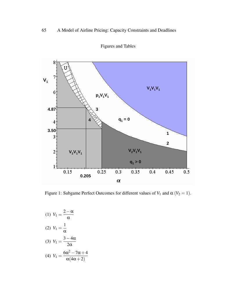
4.8 Main Results and IntuitionFigure 1 shows the pricing policies which are subgame perfect for the differentcombinations of parameter values. For higher values of V1 combined with highvalues for α, the seller chooses not to hold a ‘sale’ in any period, such that only

‘high’ valuation buyers get to purchase the good. For α ∈(

3V2

2(V1 +2V2),

2V2

V1 +V2

]the seller chooses to offer q1 = 0,q2 = 4α,q3 = 2α and to charge any price p1,p2 = p3 = V1 which is equivalent to not offering to hold a ‘sale’ in any period.For the same range of parameter values, the seller cannot choose the pricing pol-icy (V1,V1,V1,2α,2α,2α) since there exists a profitable deviation for the seller byholding a ‘sale’ in the second period and to sell to ‘high’ valuation buyers in thelast period. Had the seller been able to credibly precommit, he or she would havechosen the pricing policy (V1,V1,V1,2α,2α,2α). For lower values of α, the sellerchooses to hold a ‘sale’ in at least one period, and being patient, chooses to holda ‘sale’ in the second period. The corresponding price path was u-shaped (shadedzone in figure 1). Finally, for the lowest values of V1 and α, the seller chooses tohave a ‘sale’ in two periods and thus charges price V2 for the first two periods. 3

3Had we considered cases where ρ is much smaller than 1, we would have found combinationsof V1 and α which make (V2,V2,V2,2,1,0) subgame perfect.


[Place figure 1 here.]

Thus the main results of the theoretical model are as follows:(1) Any strategy involving a ‘sale’ in the last period is not subgame perfect. In

case the seller chooses to offer a ‘sale’ in one or both of the first two periods, themeasure of units offered for ‘sale’ is chosen in way to ensure that the measure ofunits remaining with the seller at the beginning of the third period is equal to themeasure of high type buyers who remain ‘active’ in the last period. Since p3 ∈{V1,V2}, revenue maximization in the last period requires the seller to cater only tohigh valuation buyers.

(2) The total measure of units offered in any period(s) in which a ‘sale’ is an-nounced is a decreasing function of α. This means that as the proportion of highvaluation buyers increases, the seller chooses to offer a smaller measure of units atprice V2. For example, in case the seller wants to offer p1 = p2 = V2 and p3 = V1,

then with α ∈[

14,V2

V1

]and ρ → 1, the seller offers q1 =

3−6α

1−α,q2 = 0 and with

α <14≤ V2

V1, he (she) offers q1 = 2 and q3 =

1−4α

1−α, such that (q1 + q2) was a

decreasing function of α. Similarly, for the case where the seller chooses to offer a

‘sale’ in the second period only, then with α≤ 2V2

V1 +V2and ρ→ 1, the seller offers

q2 =6α2−15α+6

2(1−α)which is also decreasing in α.

(3) The price path is horizontal, u-shaped or strictly non-decreasing for variousranges of parameter values (see figure 1).

We collected data in order to test these predictions empirically. In the event theempirical results failed to match the theoretical predictions, we attempt to providean intuitive explanation behind such a failure(s).

5 DataWhile the theoretical model was highly stylized in the sense that it allowed us tocapture certain features of the airline ticket pricing, it diverged from the airlineticket market in the following ways. First, we often observe last minute deals be-ing offered by some airlines on online travel sites like Priceline. Such discountsare never made available directly from the airlines themselves. In this case, air-lines wait till the last few days before the flight departs and offer these seats at adiscount through some online travel agents, since selling them at a lower price ispreferred to flying with empty seats. Our theoretical model did not allow for suchstrategies. Second, airline tickets usually come with various sorts of restrictions.


Travel restrictions are placed on certain tickets being offered at cheaper rates tomake them unattractive to price inelastic buyers (for example, Saturday-night stay-over). Consumers end up self selecting the type of ticket and its price which theyfind most attractive. However, the theoretical model constructed, did not allow forsuch purchase restrictions and had no quality differentiation for the product beingsold.

We collected price data for economy class tickets for one-way, non-stop flightsin the US. We thus consider tickets with the least number of restrictions. Further,these routes were hand-selected such that only a single carrier offered services oneach of them. This was done to ensure that the airline was a monopoly on thatparticular route, since the theoretical predictions are valid only for a single sellerframework and we were unsure of how the predictions would change for a multipleseller setup. Even though the theoretical model made predictions about the shapeof the price path and the measure of units made available for sale in each period fordifferent range of parameter values, we could only empirically test the predictionsabout the shape of the price path since the number of seats made available for saleby an airline over any period of time was not observable.

The data set consists of two main components. The first component containsairline pricing data on selected routes while the second describes the proportion of“high” type buyers on each of these routes.

5.1 Airline Price Data

We collected pricing data for 28 one-way, non-stop flights and for 2 two-way non-stop flights from Expedia and Orbitz. The data was collected twice a day, at 8AMand 8PM, for 14-15 weeks (except for one flight for which we have 11 weeks ofobservations), which led to a total of 6136 observations. A total of 14 airlines oper-ated on these routes which consisted of 44 distinct cities, of which some were majorplayers like American and Delta, while others were smaller carriers like MidwestAirlines and Frontier Airlines.

The routes and flights selected had the following features: (1) Each route hada single airline operating on it. (2) Routes with a single airline but with more thantwo flights operating on a single day were excluded. Routes which had two flightswhich departed within a few hours of each other were also omitted. The selectedroutes had a maximum of two flights operating on them on any given day and inthe event there was more than one flight, the flights departed at least 3 hours apart.4

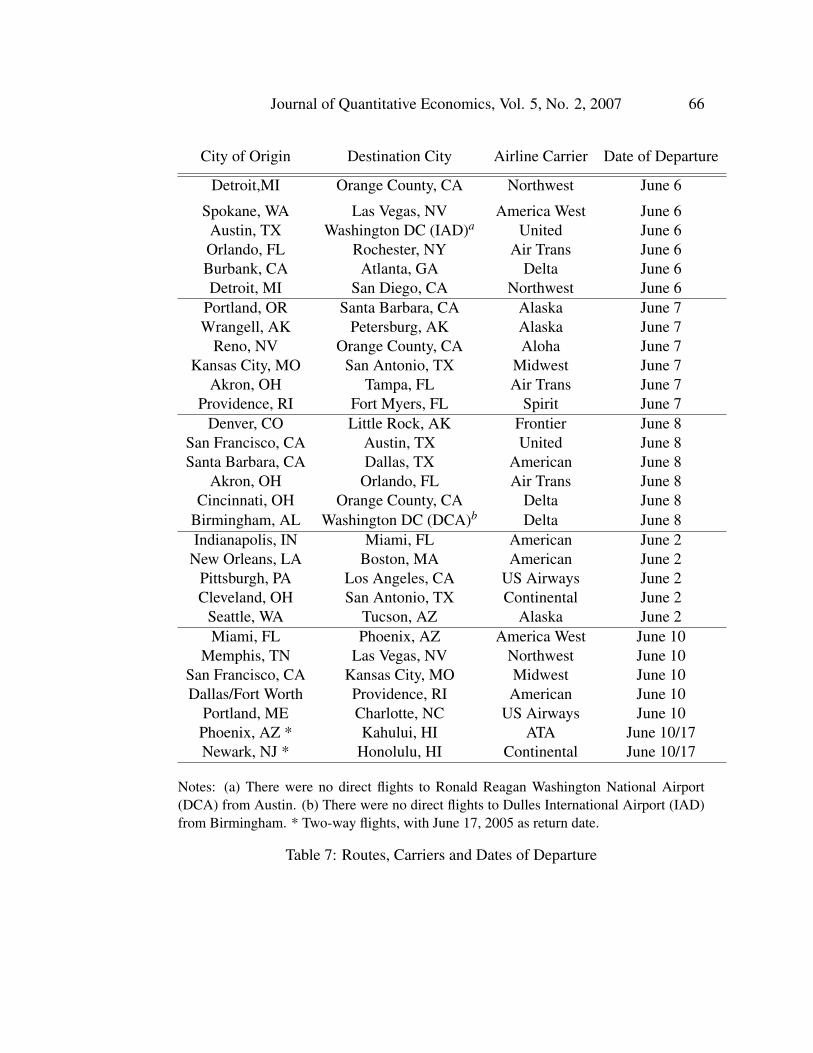
Thus, the selected flights had little or no competition.The selected routes, the carriers serving them and the dates of departure, are

4Of the 30 routes, only 5 had two flights operating on them on any given day.


listed in table 7. All flights departed in early June, 2005. The flights to Kahu-lui and Honolulu were two-way, both having return dates on June 17, 2005. Wepurposely chose these dates following an observation by Etzioni at al, that pricesbounce around more for flights leaving around holidays than others.

5.2 Data on Proportion of “High” Type BuyersWe use the American Travel Survey (ATS, 1995) as the source for data on theproportion of buyers with a higher willingness to pay. The survey contains data atthe state and metropolitan area (MA) levels and describes trip characteristics forboth households and individuals. Given a MA, trip characteristics for an individualperson are arranged in the following sequence. First, the survey reports “person tripcharacteristics” given the MA as destination and the different census divisions (CD)as origin. Second, it displays the same characteristics for the same metropolitan areaas origin and the various CDs as destination. Next, taking the MA as destination, thesurvey presents trip characteristics for the most frequent state origins. These statesare the ones with the 10 largest volumes of travel to that particular MA. Fourth,taking the MA as origin, the corresponding numbers are listed for the states whichare the top 10 destinations. Finally, the same order is followed for the cities whichare the most frequent origins and destinations for travel to and from that particularMA.

Trip characteristics amongst others included “main purpose of trip”, which wasfurther categorized into business, pleasure and others. Ideally, we would want thepercentage of travelers who traveled by plane for business purposes from one MAto another. However, these numbers were not available.

The survey also, did not report data for any of the routes on which both MAswere represented as origin and destination. Thus, while we had data for both SanFrancisco and Kansas City MAs individually, the proportion of business travelerstraveling from San Francisco to Kansas City were unavailable. This is because onone hand San Francisco was not amongst the top 10 cities having the most travelvolume going to Kansas City and on the other, Kansas City was not amongst thetop 10 cities having the most travel volume coming from San Francisco.

While we could have avoided this problem by looking at routes like New York-Boston and San Francisco-Phoenix for which we would have the correspondingpercentages of travelers traveling for business purposes, these routes had a numberof airline carriers flying on them, which made these markets oligopolies instead ofmonopolies, and unsuitable for consideration. We chose to fix the destination cityand looked at the percentages of travelers traveling for business purposes (includesall forms of transportation), from the CD to which the city of origin belonged.For example, for the flight from New Orleans to Boston, we fixed the destination


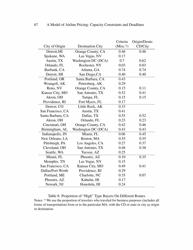
city (Boston) and looked at the proportion of business travelers traveling from theWest South Central CD to which Louisiana belongs. This meant that we could useonly 19 of the original 30 routes selected for data collection. The proportions of“business” travelers traveling on the different routes are reported in table 8.

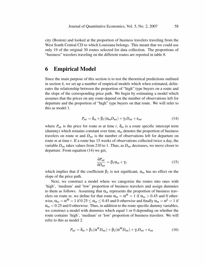
6 Empirical ModelSince the main purpose of this section is to test the theoretical predictions outlinedin section 4, we set up a number of empirical models which when estimated, delin-eates the relationship between the proportion of “high” type buyers on a route andthe slope of the corresponding price path. We begin by estimating a model whichassumes that the prices on any route depend on the number of observations left fordeparture and the proportion of “high” type buyers on that route. We will refer tothis as model 1.

Pmt = δm +β1(αmDmt)+ γ1Dmt + εmt (14)

where Pmt is the price for route m at time t, δm is a route specific intercept term(dummy) which remains constant over time, αm denotes the proportion of businesstravelers on route m and Dmt is the number of observations left for departure onroute m at time t. If a route has 15 weeks of observations collected twice a day, thevariable Dmt takes values from 210 to 1. Thus, as Dmt decreases, we move closer todeparture. From equation (14) we get,

∂Pmt

∂Dmt= β1αm + γ1 (15)

which implies that if the coefficient β1 is not significant, αm has no effect on theslope of the price path.

Next, we construct a model where we categorize the routes into ones with‘high’, ‘medium’ and ‘low’ proportion of business travelers and assign dummiesto them as follows. Assuming that αm represents the proportion of business trav-elers on route m, we define for that route αm = αH = 1 if αm > 0.45 and 0 other-wise, αm = αM = 1 if 0.25≤ αm ≤ 0.45 and 0 otherwise and finally αm = αL = 1 ifαm < 0.25 and 0 otherwise. Thus, in addition to the route specific dummy variables,we construct a model with dummies which equal 1 or 0 depending on whether theroute contains ‘high’, ‘medium’ or ‘low’ proportion of business travelers. We willrefer to this as model 2.

Pmt = δm +β1(αHDmt)+β2(αMDmt)+ γ1Dmt + εmt (16)


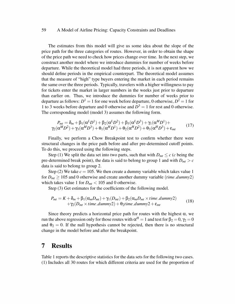
The estimates from this model will give us some idea about the slope of theprice path for the three categories of routes. However, in order to obtain the shapeof the price path we need to check how prices change over time. In the next step, weconstruct another model where we introduce dummies for number of weeks beforedeparture. While the theoretical model had three periods, it is not apparent how weshould define periods in the empirical counterpart. The theoretical model assumesthat the measure of “high” type buyers entering the market in each period remainsthe same over the three periods. Typically, travelers with a higher willingness to payfor tickets enter the market in larger numbers in the weeks just prior to departurethan earlier on. Thus, we introduce the dummies for number of weeks prior todeparture as follows: D1 = 1 for one week before departure, 0 otherwise, D2 = 1 for1 to 3 weeks before departure and 0 otherwise and D3 = 1 for rest and 0 otherwise.The corresponding model (model 3) assumes the following form.

Pmt = δm +β1(αLD1)+β2(αLD2)+β3(αLD3)+ γ1(αMD1)+γ2(αMD2)+ γ3(αMD3)+θ1(αHD1)+θ2(αHD2)+θ3(αHD3)+ εmt

(17)

Finally, we perform a Chow Breakpoint test to confirm whether there werestructural changes in the price path before and after pre-determined cutoff points.To do this, we proceed using the following steps.

Step (1) We split the data set into two parts, such that with Dmt ≤ c (c being thepre-determined break point), the data is said to belong to group 1 and with Dmt > cdata is said to belong to group 2.

Step (2) We take c = 105. We then create a dummy variable which takes value 1for Dmt ≥ 105 and 0 otherwise and create another dummy variable (time dummy2)which takes value 1 for Dmt < 105 and 0 otherwise.

Step (3) Get estimates for the coefficients of the following model.

Pmt = K +δm +β1(αmDmt)+ γ1(Dmt)+β2(αmDmt × time dummy2)+γ2(Dmt × time dummy2)+θ2time dummy2+ εmt

(18)

Since theory predicts a horizontal price path for routes with the highest α, werun the above regression only for those routes with αH = 1 and test for β2 = 0, γ2 = 0and θ2 = 0. If the null hypothesis cannot be rejected, then there is no structuralchange in the model before and after the breakpoint.

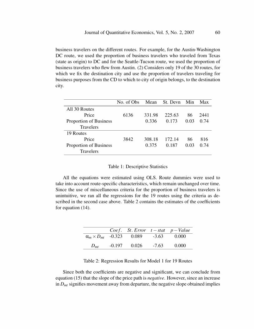
7 ResultsTable 1 reports the descriptive statistics for the data sets for the following two cases.(1) Includes all 30 routes for which different criteria are used for the proportion of


business travelers on the different routes. For example, for the Austin-WashingtonDC route, we used the proportion of business travelers who traveled from Texas(state as origin) to DC and for the Seattle-Tucson route, we used the proportion ofbusiness travelers who flew from Austin. (2) Considers only 19 of the 30 routes, forwhich we fix the destination city and use the proportion of travelers traveling forbusiness purposes from the CD to which to city of origin belongs, to the destinationcity.

No. of Obs Mean St. Devn Min MaxAll 30 Routes

Price 6136 331.98 225.63 86 2441Proportion of Business 0.336 0.173 0.03 0.74

Travelers19 Routes

Price 3842 308.18 172.14 86 816Proportion of Business 0.375 0.187 0.03 0.74

Travelers

Table 1: Descriptive Statistics

All the equations were estimated using OLS. Route dummies were used totake into account route-specific characteristics, which remain unchanged over time.Since the use of miscellaneous criteria for the proportion of business travelers isunintuitive, we ran all the regressions for the 19 routes using the criteria as de-scribed in the second case above. Table 2 contains the estimates of the coefficientsfor equation (14).

Coe f . St. Error t− stat p−Valueαm×Dmt -0.323 0.089 -3.63 0.000

Dmt -0.197 0.026 -7.63 0.000

Table 2: Regression Results for Model 1 for 19 Routes

Since both the coefficients are negative and significant, we can conclude fromequation (15) that the slope of the price path is negative. However, since an increasein Dmt signifies movement away from departure, the negative slope obtained implies


that prices increase as we move closer to departure. This result corroborates earlierfindings of Stavins (2001), McAfee and Velde (2004) and Etzioni et al (2003).

The coefficients of model 2 could be interpreted as follows. Each route can onlyhave either high, medium or low proportion of travelers with a high valuation. Thecoefficient for Dmt represents the base case and denotes the slope of the price pathfor routes which have αm = αL (second and third terms drop out). The sum of thecoefficients of αM ×Dmt and Dmt refers to the slope of the price path for routeswith αm = αM, while the sum of the coefficients of αH ×Dmt and Dmt representsthe slope of the price path for routes with αm = αH .

Coe f . St. Error t− stat p−ValueαH ×Dmt -.215 .056 -3.85 0.000

αM×Dmt .060 .033 1.81 0.071

Dmt -.277 .021 -13.30 0.000


Thus, the slopes of the price path for routes with low, medium and high propor-tion of travelers with a high valuation are−0.277,−0.217 and−0.492 respectively.Prices are found to increase most quickly in routes with the highest proportion ofbusiness travelers.

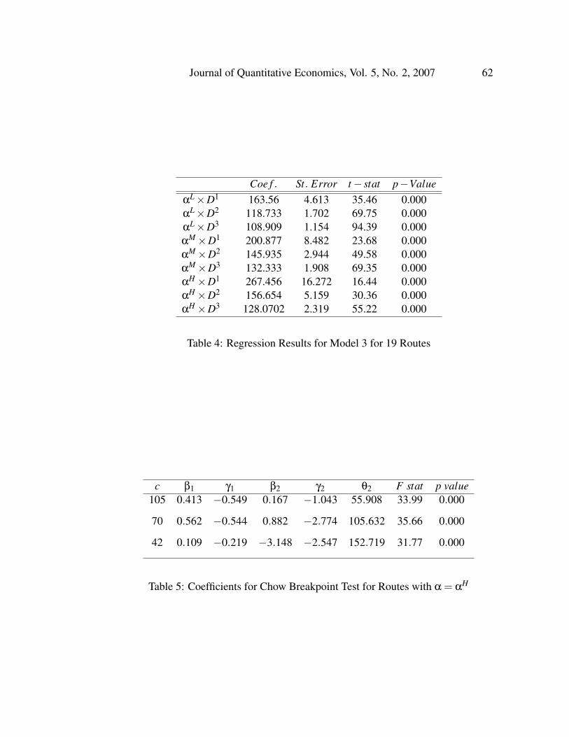
The coefficients of model 3 allows us to demonstrate the relationship betweenthe shape of the price path and the corresponding αm. The price path is found to berising for all three categories of routes (table 4). Routes with αm = αH shows thesharpest increase in prices. The theoretical prediction that the price path for routeswith high α is horizontal is thus found to be empirically invalid.

Finally, we report the results for the Chow Breakpoint test. For routes withα = αH , theory predicts that there will be no change in the slope or the interceptbefore and after the break point. This implies that all three coefficients β2,γ2 and θ2need to be not significant for equation (18). Table 5 reports the coefficients for theChow Breakpoint test for different pre-determined cutoff values (c). The F-statisticis based on the null hypothesis which involves the restrictions, β2 = 0,γ2 = 0 andθ2 = 0. The low p-values led us to conclude that the null hypothesis can be rejectedfor all three pre-determined cutoff points and that there is structural change in themodel before and after these cutoff points.

Next, we collect empirical evidence which establishes that the shape of the price


Coe f . St. Error t− stat p−ValueαL×D1 163.56 4.613 35.46 0.000αL×D2 118.733 1.702 69.75 0.000αL×D3 108.909 1.154 94.39 0.000αM×D1 200.877 8.482 23.68 0.000αM×D2 145.935 2.944 49.58 0.000αM×D3 132.333 1.908 69.35 0.000αH ×D1 267.456 16.272 16.44 0.000αH ×D2 156.654 5.159 30.36 0.000αH ×D3 128.0702 2.319 55.22 0.000


c β1 γ1 β2 γ2 θ2 F stat p value105 0.413 −0.549 0.167 −1.043 55.908 33.99 0.000

70 0.562 −0.544 0.882 −2.774 105.632 35.66 0.000

42 0.109 −0.219 −3.148 −2.547 152.719 31.77 0.000

Table 5: Coefficients for Chow Breakpoint Test for Routes with α = αH


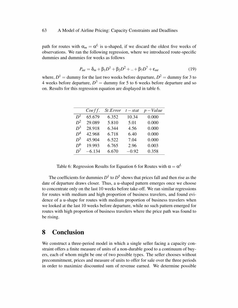
path for routes with αm = αL is u-shaped, if we discard the oldest five weeks ofobservations. We ran the following regression, where we introduced route-specificdummies and dummies for weeks as follows

Pmt = δm +β1D1 +β2D2 + ..+β7D7 + εmt (19)

where, D1 = dummy for the last two weeks before departure, D2 = dummy for 3 to4 weeks before departure, D3 = dummy for 5 to 6 weeks before departure and soon. Results for this regression equation are displayed in table 6.

Coe f f . St.Error t− stat p−ValueD1 65.679 6.352 10.34 0.000D2 29.089 5.810 5.01 0.000D3 28.918 6.344 4.56 0.000D4 42.968 6.718 6.40 0.000D5 45.904 6.522 7.04 0.000D6 19.993 6.765 2.96 0.003D7 −6.134 6.670 −0.92 0.358

Table 6: Regression Results for Equation 6 for Routes with α = αL

The coefficients for dummies D1 to D5 shows that prices fall and then rise as thedate of departure draws closer. Thus, a u-shaped pattern emerges once we chooseto concentrate only on the last 10 weeks before take-off. We ran similar regressionsfor routes with medium and high proportion of business travelers, and found evi-dence of a u-shape for routes with medium proportion of business travelers whenwe looked at the last 10 weeks before departure, while no such pattern emerged forroutes with high proportion of business travelers where the price path was found tobe rising.

8 ConclusionWe construct a three-period model in which a single seller facing a capacity con-straint offers a finite measure of units of a non-durable good to a continuum of buy-ers, each of whom might be one of two possible types. The seller chooses withoutprecommitment, prices and measure of units to offer for sale over the three periodsin order to maximize discounted sum of revenue earned. We determine possible


shapes of the corresponding price path for different values of the parameters andfind that for certain combinations of the parameter values, the optimal price pathis u-shaped. For other combinations, we find that the optimal price path is eitherstrictly non-decreasing (which is consistent with a result in a paper by Stavins) orhorizontal.

While the theoretical prediction that prices never fall before departure was cor-roborated, the prediction that the price path for routes with the highest proportionof “high” type buyers is horizontal was found to be empirically invalid. Instead,routes with high proportions of business travelers witnessed the steepest increase inprices. The price path for the routes with low and medium proportions of businesstravelers was also found to be increasing.

In our theoretical model we assumed that the proportion of buyers with a highervaluation for the good, who enters the market in each period, remains constant overthe three periods. In reality, this is clearly not the case. It is our conjecture thata theoretical model which allows for variation in the proportion of high valuationbuyers over the three periods, where the proportion increases from the first to thethird period, will perform better in terms of providing an explanation for the empir-ical results. However, even if we do solve for the price paths for various parametervalues for such a model, it will be difficult to access data which describe how theproportion of travelers traveling for business purposes on different routes change asthe date of departure draws closer.

The theoretical model also predicted a small range of parameter values forwhich the price path would be u-shaped. While we did find some empirical evi-dence for a u-shaped price path for routes with low or medium proportion of highvaluation buyers, we did so only after truncating the data and considering the last10 weeks of observations.


Figures and Tables

V2V1V1

V1V1V1

p1V1V1

q1 = 0

V2V1V1

q1 > 0

1

2

3

4

V1

0.205

4.87

3.50

Figure 1: Subgame Perfect Outcomes for different values of V1 and α (V2 = 1).

(1) V1 =2−α

α

(2) V1 =1α

(3) V1 =3−4α

2α

(4) V1 =6α2−7α+4

α(4α+2)


City of Origin Destination City Airline Carrier Date of Departure

Detroit,MI Orange County, CA Northwest June 6

Spokane, WA Las Vegas, NV America West June 6Austin, TX Washington DC (IAD)a United June 6Orlando, FL Rochester, NY Air Trans June 6Burbank, CA Atlanta, GA Delta June 6Detroit, MI San Diego, CA Northwest June 6

Portland, OR Santa Barbara, CA Alaska June 7Wrangell, AK Petersburg, AK Alaska June 7

Reno, NV Orange County, CA Aloha June 7Kansas City, MO San Antonio, TX Midwest June 7

Akron, OH Tampa, FL Air Trans June 7Providence, RI Fort Myers, FL Spirit June 7

Denver, CO Little Rock, AK Frontier June 8San Francisco, CA Austin, TX United June 8Santa Barbara, CA Dallas, TX American June 8

Akron, OH Orlando, FL Air Trans June 8Cincinnati, OH Orange County, CA Delta June 8

Birmingham, AL Washington DC (DCA)b Delta June 8Indianapolis, IN Miami, FL American June 2

New Orleans, LA Boston, MA American June 2Pittsburgh, PA Los Angeles, CA US Airways June 2Cleveland, OH San Antonio, TX Continental June 2

Seattle, WA Tucson, AZ Alaska June 2Miami, FL Phoenix, AZ America West June 10

Memphis, TN Las Vegas, NV Northwest June 10San Francisco, CA Kansas City, MO Midwest June 10Dallas/Fort Worth Providence, RI American June 10

Portland, ME Charlotte, NC US Airways June 10Phoenix, AZ * Kahului, HI ATA June 10/17Newark, NJ * Honolulu, HI Continental June 10/17

Notes: (a) There were no direct flights to Ronald Reagan Washington National Airport(DCA) from Austin. (b) There were no direct flights to Dulles International Airport (IAD)from Birmingham. * Two-way flights, with June 17, 2005 as return date.

Table 7: Routes, Carriers and Dates of Departure


Criteria Origin/Destn:City of Origin Destination City (Misc.*) CD/City

Detroit,MI Orange County, CA 0.46 0.46Spokane, WA Las Vegas, NV 0.17Austin, TX Washington DC (DCA) 0.7 0.62Orlando, FL Rochester, NY 0.03 0.03Burbank, CA Atlanta, GA 0.74 0.74Detroit, MI San Diego,CA 0.40 0.40

Portland, OR Santa Barbara, CA 0.43Wrangell, AK Petersburg, AK 0.29

Reno, NV Orange County, CA 0.15 0.11Kansas City, MO San Antonio, TX 0.52 0.41

Akron, OH Tampa, FL 0.15 0.15Providence, RI Fort Myers, FL 0.17

Denver, CO Little Rock, AK 0.33San Francisco, CA Austin, TX 0.41Santa Barbara, CA Dallas, TX 0.55 0.52

Akron, OH Orlando, FL 0.23 0.23Cincinnati, OH Orange County, CA 0.42 0.46

Birmingham, AL Washington DC (DCA) 0.43 0.43Indianapolis, IN Miami, FL 0.06 0.45

New Orleans, LA Boston, MA 0.55 0.55Pittsburgh, PA Los Angeles, CA 0.27 0.37Cleveland, OH San Antonio, TX 0.48 0.38

Seattle, WA Tucson, AZ 0.25Miami, FL Phoenix, AZ 0.10 0.35

Memphis, TN Las Vegas, NV 0.15San Francisco, CA Kansas City, MO 0.49 0.41Dallas/Fort Worth Providence, RI 0.29

Portland, ME Charlotte, NC 0.35 0.07Phoenix, AZ Kahului, HI 0.17Newark, NJ Honolulu, HI 0.24

Table 8: Proportion of “High” Type Buyers On Different RoutesNotes: * We use the proportion of travelers who traveled for business purposes (includes allforms of transportation) from or to the particular MA, with the CD or state or city as originor destination.


References[1] Brumelle, S.L. and McGill, J.I. “Airline Seat Allocation with Multiple Nested

Fare Classes”, Operations Research, Vol. 41, No. 1, Special Issue on Stochas-tic and Dynamic Models in Transportation (Jan - Feb, 1993), 127-137.

[2] Coase, Ronald H. “Durability and Monopoly”, Journal of Law and Eco-nomics, Vol. 15, (April 1972), 143-149.

[3] Conlisk, John, Gerstner, Eitan and Sobel, Joel “Cyclic Pricing by a DurableGoods Monopolist”, Quarterly Journal of Economics, Vol. 99, Issue 3 (August1984), 489-505.

[4] Etzioni, Oren, Knoblock, Craig, Tuchinda, Rattapoom and Yates, Alexander“To Buy or Not to Buy: Mining Airline Fare Data to Minimize Ticket Pur-chase Price”, Proceeding of the 9th ACM SIGKDD International Conferenceon Knowledge Discovery and Data Mining, Washington DC.

[5] Kreps, David M. and Scheinkman, Jose A. “Quantity Precommitment andBertrand Competition Yield Cournot Outcomes”, Bell Journal of Economics,Vol. 14, No. 2 (Autumn 1983), 326-337.

[6] McAfee, Preston R. and Velde, te Vera “Dynamic Pricing in the Airline In-dustry”, California Institute of Technology, mimeo.

[7] McAfee, Preston R. and Wiseman, Thomas “Capacity Choice Counters theCoase Conjecture”, July 25, 2003.

[8] Narasimhan, Chakravarthi “Incorporating Consumer Price Expectations inDiffusion Models”, Marketing Science, Vol. 8, No. 4 (Autumn 1989), 343-357.

[9] Sobel, Joel “The Timing of Sales”, Review of Economic Studies, Vol. 51,Issue 3 (July 1984), 353-368.

[10] Stavins, Joanna “Price Discrimination in the Airline Market: The Effect ofMarket Concentration”, Review of Economics and Statistics, Vol. 83, No. 1(February 2001).

[11] Wollmer, Richard D. “An Airline Seat Management Model for a Single LegRoute When Lower Fare Classes Book First”, Operations Research, Vol. 40,No. 1, (Jan - Feb, 1992), 26-37.

Documents

A Model of Airline Pricing: Capacity Constraints and · PDF file41 A Model of Airline Pricing: Capacity Constraints and Deadlines to departure, prices start rising. Instead of monotonically