A Method to Calculate Uncertainty of Empirical Compressor ... · measurements of compressor suction and discharge pressure in calorimeter tests and are commonly used by compressor

Postprint for doi: 10.1080/23744731.2017.1372805

Cheung, H., Sarfraz, O. and Bach, C. K.

1

A Method to Calculate Uncertainty of Empirical Compressor

Maps with the Consideration of Extrapolation Effect and

Choice of Training Data

Although compressor maps are powerful tools to estimate compressor power consumption quickly, their

ability to extrapolate outside their training data range is always questioned. In order to quantify the effect

of extrapolation, a method to calculate the uncertainty of compressor map outputs is develo ped in this

paper. The method considers 4 major components of uncertainties due to various sources such as

measurement uncertainties of training data and equation of state. The change of the predicted map

uncertainty with the degree of extrapolation and the map accuracy are shown for 8 different compressor

maps. The results indicate that the uncertainty from model random error increases significantly as the

maps extrapolate though extrapolation does not necessarily imply inaccurate compressor map outputs. The

results also show that the uncertainty due to training data is the most significant component of

uncertainties when the maps are not extrapolated.

Introduction and Literature Review

Compressor models are widely used in specifying the performance of compressors by manufacturers

for design purposes of compressors as well as for vapor compression system simulation. When models are

built for compressor designs, deterministic models such as e.g. Wang et al. (2008), Bell et al. (2012), Gall

et al. (2015) and Ibsaine et al. (2016) are used because the models give them flexibility to optimize a

compressor design by tuning the geometry of the compressors and compressor valves and allows the

investigators to study the compressor dynamics in details. However, modelers of thermal systems using

compressors do not need the flexibility because changes of compressor geometry are usually not concerns

of the system modelers (Ding 2007), nor do they need the study of the compressor dynamics because heat

exchanger dynamics are usually more important in their applications (Rasmussen 2012). While models of

some types of compressors can be simplified for their uses as subsystem models (Wang et al. 2000), others

who cannot simplify the deterministic models such as ones of scroll compressors prefer to use simplified

compressor models trained by experimental data. This speeds up their models which require multiple runs



2

of the compressor model for one run of their system models (Park et al. 2001; Zakula et al. 2011; Cheung

and Braun 2013; Heo et al. 2013). The simplest compressor map has standard forms (e.g. AHRI Standard

540 (AHRI 2004), EN Standard 12900 (CEN 2013)) that can be constructed easily by linear regression with

measurements of compressor suction and discharge pressure in calorimeter tests and are commonly used by

compressor manufacturers to describe their compressor performance in specifications and reports (AHRI,

2016).

The performance of mappings is commonly expressed in terms of the accuracy of the maps at training

data points. This can be easily done and therefore used widely for conventional compressors (e.g. Jähnig et

al. 2000; Winandy et al. 2002), variable speed compressors (e.g. Shao et al. 2004), as well as for

compressors with injection (e.g. Navarro et al. 2013; Bach et al. 2015; Dardenne et al. 2015).

Although the performance accessed by prediction accuracy at training data points is easy for readers to

understand, they do not account for the effect of the measurement uncertainty of the training data. They

also do not specify the effect of the choice of training data to the accuracy of the maps (e.g. the change of

map accuracy due to the change of the training data set). It is typically unclear if the maps are accurate

outside their training data range before any experimental validation, and this lack of knowledge may cost

opportunities in compressor model development such as the possibility to reduce the number of calorimeter

tests with correct choices of calorimeter test conditions and the option of validation o f compressor map

outputs for out-of-range operation without extra testing. This also hinders the research development using

compressor maps such as cold climate heat pump (Caskey et al. 2012) and faulted vapor compression

systems (Shen et al. 2009) which involves the use of compressor maps at out-of-range operation.

Few research papers investigate the issue of map performance outside the range of training data. Jähnig

et al (2000) conducted a rigorous study in which they showed that map performance outside of the training

data range can drastically differ from the performance within the training data range. The authors did extra

tests to define the extrapolation accuracy of the map to be within 10% of the measurement when the

evaporating and condensing temperature lied within 10 K (18°R) from the extremes in the training data, but

it is unknown how the magnitude of the temperature difference 10 K (18°R) is coupled with the range of

the saturation temperature in the training data. Li (2012) did a similar study for its scroll and reciprocating

compressor model. Aute et al. (2015) compared various compressor modeling methods and used Monte



3

Carlo method to calculate the uncertainty of 10-coefficient compressor maps, but its method from Coleman

and Steele (2009) does not involve the difference between model training data and model inputs and cannot

account for the effect of extrapolation to model uncertainties well. Their method also requires more than

1,000 runs of the map and its training process to calculate the uncertainty per data point is not very feasible

for most applications.

It is usually believed that extrapolation error might be reduced by using deterministic models, such as

ones in Wang et al. (2008), Bell et al. (2012), and Molinaroli et al. (2017), which are tuned or scaled

towards the experimental data. However, these deterministic models are often not used in developments

that require quantification of extrapolation errors because of the aforementioned reasons, and another

approach is needed to quantify the potential extrapolation error.

To simplify the quantification of extrapolation error for empirical compressor maps, Cheung and Bach

(2015) proposed a method to break up overall compressor power consumption uncertainty into four

contribution components. The authors compared the actual accuracy of the map to the sum of the

uncertainty contribution components and found that both increase if the number of training data points is

decreased. Uncertainty was found to increase with increasing distance from the nearest training data point.

Bach and Cheung (2015) extended the method in Cheung and Bach (2015) towards data from a vapor

injected compressor. However, both papers were developed on either simulation results only or the

performance of specialized models. A more rigorous method that is validated by experimental results and a

more general method of compressor map uncertainty prediction is therefore needed.

This paper focuses on the development and application of a rigorous approach taking into account a ll

major aspects and sources of the uncertainties involved in 10-coefficient compressor map in AHRI

Standard 540 (AHRI 2010) that predicts compressor power consumption. The map is widely used in the

community for various applications (e.g. use of the compressor maps in reports to compare performance of

compressors using various refrigerants from different manufacturers in AHRI 2016; use of the compressor

map in cold climate heat pump studies in Caskey et al. 2012; use of the compressor map for vapor

compression system design in Rice and Jackson 2005; use of the compressor map for faulted vapor

compression systems in Shen et al. 2009; study of the uncertainty of the compressor map with a numerical

approach in Aute et al. 2015) and are useful to illustrate the quantification of extrapolation effect by



4

uncertainty calculation. In particular, it breaks out the effect of different uncertainty components, including

pressure measurement, equation of state, model random error, training data, and outputs. This breakdo wn

allows to specify the major sources of uncertainty and their effects due to changes in the training data,

which can be used to simplify the calculation of these components further in future works.

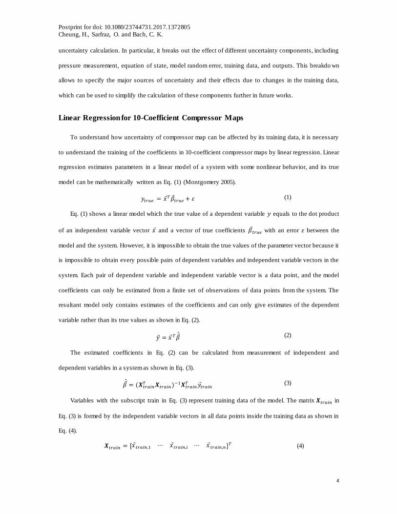
Linear Regression for 10-Coefficient Compressor Maps

To understand how uncertainty of compressor map can be affected by its training data, it is necessary

to understand the training of the coefficients in 10-coefficient compressor maps by linear regression. Linear

regression estimates parameters in a linear model of a system with some nonlinear behavior, and its true

model can be mathematically written as Eq. (1) (Montgomery 2005).

𝑦𝑡𝑟𝑢𝑒 = 𝑥𝑇 ��𝑡𝑟𝑢𝑒 + 𝜀 (1)

Eq. (1) shows a linear model which the true value of a dependent variable 𝑦 equals to the dot product

of an independent variable vector 𝑥 and a vector of true coefficients 𝛽𝑡𝑟𝑢𝑒 with an error 𝜀 between the

model and the system. However, it is impossible to obtain the true values of the parameter vector because it

is impossible to obtain every possible pairs of dependent variables and independent variable vectors in the

system. Each pair of dependent variable and independent variable vector is a data point, and the model

coefficients can only be estimated from a finite set of observations of data points from the system. The

resultant model only contains estimates of the coefficients and can only give estimates of the dependent

variable rather than its true values as shown in Eq. (2).

𝑦 = 𝑥 𝑇 �� (2)

The estimated coefficients in Eq. (2) can be calculated from measurement of independent and

dependent variables in a system as shown in Eq. (3).

𝛽= (𝑿𝑡𝑟𝑎𝑖𝑛

𝑇 𝑿𝑡𝑟𝑎𝑖𝑛)−1𝑿𝑡𝑟𝑎𝑖𝑛

𝑇 𝑦𝑡𝑟𝑎𝑖𝑛 (3)

Variables with the subscript train in Eq. (3) represent training data of the model. The matrix 𝑿𝑡𝑟𝑎𝑖𝑛 in

Eq. (3) is formed by the independent variable vectors in all data points inside the training data as shown in

Eq. (4).

𝑿𝑡𝑟𝑎𝑖𝑛 = [𝑥𝑡𝑟𝑎𝑖𝑛,1 ⋯ 𝑥𝑡𝑟𝑎𝑖𝑛,𝑖 ⋯ 𝑥𝑡𝑟𝑎𝑖𝑛,𝑛]𝑇 (4)



5

The vector of dependent variables of training data in Eq. (3) is also defined in a similar manner as Eq.

(5) .

𝑦𝑡𝑟𝑎𝑖𝑛 = [𝑦𝑡𝑟𝑎𝑖𝑛 ,1 ⋯ 𝑦𝑡𝑟𝑎𝑖𝑛 ,𝑖 ⋯ 𝑦𝑡𝑟𝑎𝑖𝑛 ,𝑛]𝑇 (5)

A 10-coefficient compressor map that estimates compressor power consumption is a cubic polynomial

that depends on dew point temperature values at compressor suction and discharge as shown in Eq. (6).

��𝑐𝑜𝑚𝑝 = ��0 + ��1𝑇𝑑𝑒𝑤,𝑠𝑢𝑐 + ��2𝑇𝑑𝑒𝑤,𝑑𝑖𝑠 + ��3𝑇𝑑𝑒𝑤,𝑠𝑢𝑐2 + ��4𝑇𝑑𝑒𝑤,𝑠𝑢𝑐𝑇𝑑𝑒𝑤 ,𝑑𝑖𝑠

+ ��5𝑇𝑑𝑒𝑤,𝑑𝑖𝑠2 + ��6𝑇𝑑𝑒𝑤,𝑠𝑢𝑐

3 + ��7𝑇𝑑𝑒𝑤,𝑠𝑢𝑐2 𝑇𝑑𝑒𝑤,𝑑𝑖𝑠

+ ��8𝑇𝑑𝑒𝑤,𝑠𝑢𝑐𝑇𝑑𝑒𝑤 ,𝑑𝑖𝑠2 + ��9𝑇𝑑𝑒𝑤,𝑑𝑖𝑠

3

(6)

Although the polynomial is not a simple linear equation, its empirical coefficients can still be estimated

by linear regression. To estimate the parameters in the 10-coefficient compressor map by linear regression,

the map is converted to the equation form Eq. (2) by using the independent variable vector in Eq. (7) and

the power consumption as the dependent variable.

𝑥

= [1 𝑇𝑑𝑒𝑤,𝑠𝑢𝑐 𝑇𝑑𝑒𝑤,𝑑𝑖𝑠 𝑇𝑑𝑒𝑤 ,𝑠𝑢𝑐2 𝑇𝑑𝑒𝑤,𝑠𝑢𝑐𝑇𝑑𝑒𝑤,𝑑𝑖𝑠 𝑇𝑑𝑒𝑤 ,𝑑𝑖𝑠

2 𝑇𝑑𝑒𝑤 ,𝑠𝑢𝑐3 𝑇𝑑𝑒𝑤 ,𝑠𝑢𝑐

2 𝑇𝑑𝑒𝑤,𝑑𝑖𝑠 𝑇𝑑𝑒𝑤,𝑠𝑢𝑐𝑇𝑑𝑒𝑤 ,𝑑𝑖𝑠2 𝑇𝑑𝑒𝑤 ,𝑑𝑖𝑠

3 ]𝑇

(7)

The coefficients in Eq. (6) can then be calculated by Eq. (3). Occasionally the inversion of matrices in

Eq. (3) may yield incorrect answers in computers due to numerical round-off errors, and normalization of

Eq. (7) may be needed to calculate the correct parameters. In this case, the normalized vector 𝑥 should be

used in all uncertainty calculation methods in this paper in order to calculate the correct uncertainties and

estimation.

Although the map uses dew point temperature at compressor suction and discharge, they are not

measured directly from the compressor. In reality, only refrigerant pressure values at compressor suction

and discharge are measured, and then converted to compressor suction and discharge dew point

temperature before being used by the maps to calculate compressor power consumption.

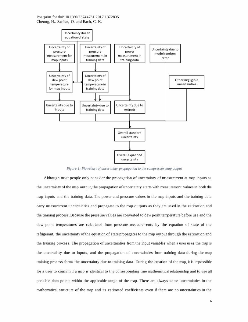
Method to Calculate Uncertainty of Compressor Map Output

Uncertainty of the compressor map output quantifies the potential difference between the true values of

the output to the map outputs. The sources of uncertainty propagated to the map output are illustrated in

Figure 1.



6

Figure 1: Flowchart of uncertainty propagation to the compressor map output

Although most people only consider the propagation of uncertainty of measurement at map inputs as

the uncertainty of the map output, the propagation of uncertainty starts with measurement values in both the

map inputs and the training data. The power and pressure values in the map inputs and the training data

carry measurement uncertainties and propagate to the map outputs as they are us ed in the estimation and

the training process. Because the pressure values are converted to dew point temperature before use and the

dew point temperatures are calculated from pressure measurements by the equation of state of the

refrigerant, the uncertainty of the equation of state propagates to the map output through the estimation and

the training process. The propagation of uncertainties from the input variables when a user uses the map is

the uncertainty due to inputs, and the propagation of uncertaint ies from training data during the map

training process forms the uncertainty due to training data. During the creation of the map, it is impossible

for a user to confirm if a map is identical to the corresponding true mathematical relationship and to use a ll

possible data points within the applicable range of the map. There are always some uncertainties in the

mathematical structure of the map and its estimated coefficients even if there are no uncertainties in the

Uncertainty of pressure

measurement in training data

Uncertainty due to equation of state

Uncertainty due to inputs

Uncertainty due to training data

Uncertainty due to outputs

Uncertainty of power


Other negligible uncertainties

Uncertainty due to model random

error

Overall standard uncertainty

Overall expanded uncertainty

Uncertainty of dew point

temperature for map inputs


measurement for map inputs


temperature in training data



7

measurement and equation of state, and it is proposed to account for this type of uncertainty by calculating

the uncertainty due to model random error. Since the map is trained by measured values of the variables,

the uncertainty components only account for the uncertainty between the map estimation and the

corresponding measurement. However, the uncertainty of a sensor is the uncertainty between the

measurement and the corresponding true value, and hence the uncertainty of a map output should be

defined similarly as the uncertainty between the estimation and the corresponding true value, and an

uncertainty component called the uncertainty due to outputs is introduced to satisfy this definition. . These

uncertainties together form the uncertainty due to inputs, the uncertainty due to training data, the

uncertainty due to model random error, and the uncertainty due to outputs. The imperfection of the cubic

compressor map and the training data to represent the compressor power in the entire operating range of the

compressor forms the uncertainty from model random error.

There are other sources of uncertainties that are neglected in this study. For example, although the

uncertainty due to numerical approximation exists because of the numerical procedure used in the

calculation of the compressor map, they are assumed to be negligible because the solution of the

polynomial is explicit and is not complex. Uncertainties due to manufacturing tolerances, aging, and wear

are also neglected in the current work because data on these issues in public literature is limited.

The combination of the four remaining major uncertainty components - uncertainty due to inputs,

uncertainty due to training data, uncertainty due to outputs, and uncertainty due to model random error -

creates the overall standard uncertainty of the compressor map output, which can be expanded to the

overall expanded uncertainty by defining a confidence level as suggested in ASME Performance Test

Codes (PTC) 19.1-2013 (ASME 2013).

Uncertainty of pressure measurement

Uncertainty of pressure measurement ∆𝑃𝑚𝑒𝑎 is usually described as a percentage 𝑟𝑝 of full scale

measurement 𝑃𝑓𝑢𝑙𝑙 in the specification of a pressure transducer. It can be calculated by Eq. (8).

∆𝑃𝑚𝑒𝑎 = 𝑟𝑃𝑃𝑓𝑢𝑙𝑙 (8)

For uncertainties that are decscribed as the percentage of measured pressure rmea, Eq. (9) can be used

.



8

∆𝑃𝑚𝑒𝑎 = 𝑟𝑚𝑒𝑎𝑃𝑚𝑒𝑎 (9)


Uncertainty of equation of states is the uncertainty of the estimation equation of dew point temperature

from pressure, and it differs between equations of states. Its values for different refrigerants are tabulated in

Table 1.

Table 1: Uncertainty of equations of states of different

refrigerant

Refrigerant Uncertainty Literature

R22 0.2% of the dew point pressure Kamei et al. (1995)

R404A 0.5% of the dew point pressure Lemmon (2003)


The uncertainty of dew point pressure due to the equation of states can be expressed by Eq. (10).

∆𝑃𝐸𝑂𝑆 = 𝑟𝐸𝑂𝑆𝑃𝑚𝑒𝑎 (10)

Uncertainty of dew point temperature

The uncertainty of dew point temperature is formed by combining the uncertainty of pressure

measurement and uncertainty due to equation of state. Assuming that the two uncertainties are not

correlated, the low-order uncertainty of dew point temperature can be computed by Eq. (11) according to

Joint Committee for Guides in Metrology (JCGM) Guide to the Expression of Uncertainty Measurement

(GUM) 100-2008 (JCGM 2008).

∆𝑇𝑑𝑒𝑤 ,𝑙𝑜𝑤 = √(𝜕𝑇𝑑𝑒𝑤 (𝑃𝑚𝑒𝑎 )

𝜕𝑃)2

⋅ (∆𝑃𝑚𝑒𝑎2 + ∆𝑃𝐸𝑂𝑆

2 )

(11)

The high-order uncertainty can be calculated by Eq. (12) following the same standard.

∆𝑇𝑑𝑒𝑤 ,ℎ𝑖𝑔ℎ = √1

2(𝜕2𝑇𝑑𝑒𝑤 (𝑃𝑚𝑒𝑎 )

𝜕𝑃2)

2

⋅ (∆𝑃𝑚𝑒𝑎4 + ∆𝑃𝐸𝑂𝑆

4 )

(12)

Although JCGM GUM 100-2008 recommends the use of third-order partial derivatives to calculate the

high-order uncertainty, they are difficult to be calculated for equation of states and are assumed to be

negligible in this paper.



9

The partial derivatives in Eq. (11) and (12) are calculated by the method in Thorade and Saadat (2013),

and the calculation is implemented by the software CoolProp (Bell et al. 2014). The overall standard

uncertainty of the dew point temperature is the sum of squares of the uncertainty component in Eq. (11) and

(12) as shown in Eq. (13).

∆𝑇𝑑𝑒𝑤 = √Δ𝑇𝑑𝑒𝑤 ,𝑙𝑜𝑤2 +Δ𝑇𝑑𝑒𝑤 ,ℎ𝑖𝑔ℎ

2 (13)


Uncertainties of inputs to the compressor map - compressor suction and discharge dew point

temperature - propagate to the map output and form the uncertainty due to inputs. According to the Joint

Committee for Guides in Metrology (JCGM) Guide to the Expression of Uncertainty Measurement (GUM)

100-2008 (JCGM 2008), the low-order uncertainty due to inputs can be calculated by Eq. (14).

∆��𝑐𝑜𝑚𝑝 ,𝑖𝑛𝑝𝑢𝑡,𝑙𝑜𝑤 = √(𝜕��𝑐𝑜𝑚𝑝

𝜕𝑇𝑑𝑒𝑤,𝑠𝑢𝑐)

2

∆𝑇𝑑𝑒𝑤,𝑠𝑢𝑐2 + (

𝜕��𝑐𝑜𝑚𝑝

𝜕𝑇𝑑𝑒𝑤,𝑑𝑖𝑠)

2

∆𝑇𝑑𝑒𝑤,𝑑𝑖𝑠2

(14)

The low-order uncertainty in Eq. (14) calculates the uncertainty due to inputs accurately if the map is

linear and hence a first-order polynomial. However, compressor map is a cubic and a high -order

polynomial. According to the JCGM GUM 100-2008, there may be a significant uncertainty component as

a result of the high-order terms. The component is labeled as high-order uncertainty due to inputs and is

calculated by Eq. (15).

∆��𝑐𝑜𝑚𝑝 ,𝑖𝑛𝑝𝑢𝑡 ,ℎ𝑖𝑔ℎ =

√

((𝜕2 ��𝑐𝑜𝑚𝑝

𝜕𝑇𝑑𝑒𝑤,𝑠𝑢𝑐 𝜕𝑇𝑑𝑒𝑤,𝑑𝑖𝑠

)

2

+𝜕��𝑐𝑜𝑚𝑝

𝜕𝑇𝑑𝑒𝑤 ,𝑠𝑢𝑐

𝜕3 ��𝑐𝑜𝑚𝑝

𝜕𝑇𝑑𝑒𝑤,𝑠𝑢𝑐 𝜕𝑇𝑑𝑒𝑤,𝑑𝑖𝑠

2


𝜕𝑇𝑑𝑒𝑤,𝑑𝑖𝑠

𝜕3��𝑐𝑜𝑚𝑝

𝜕𝑇𝑑𝑒𝑤 ,𝑠𝑢𝑐2 𝜕𝑇𝑑𝑒𝑤,𝑑𝑖𝑠

)∆𝑇𝑑𝑒𝑤,𝑠𝑢𝑐

2 ∆𝑇𝑑𝑒𝑤,𝑑𝑖𝑠2

+(1

2(𝜕2 ��𝑐𝑜𝑚𝑝

𝜕𝑇𝑑𝑒𝑤,𝑠𝑢𝑐2

)

2


𝜕𝑇𝑑𝑒𝑤,𝑠𝑢𝑐


𝜕𝑇𝑑𝑒𝑤 ,𝑠𝑢𝑐3

)∆𝑇𝑑𝑒𝑤,𝑠𝑢𝑐4

+(1

2(𝜕2 ��𝑐𝑜𝑚𝑝

𝜕𝑇𝑑𝑒𝑤,𝑑𝑖𝑠2

)

2


𝜕𝑇𝑑𝑒𝑤,𝑑𝑖𝑠


𝜕𝑇𝑑𝑒𝑤 ,𝑑𝑖𝑠3

)∆𝑇𝑑𝑒𝑤 ,𝑑𝑖𝑠4

(15)

The partial derivatives in Eq. (14) and (15) are calculated analytically by taking the partial derivative

of the compressor map with respect to the compressor suction and discharge dew point temperature.



10

The uncertainty due to inputs is the sum of the low-order and high-order uncertainties and can be

calculated by Eq. (16).

∆��𝑐𝑜𝑚𝑝 ,𝑖𝑛𝑝𝑢𝑡 = √∆��𝑐𝑜𝑚𝑝 ,𝑖𝑛𝑝𝑢𝑡,𝑙𝑜𝑤2 +∆��𝑐𝑜𝑚𝑝 ,𝑖𝑛𝑝𝑢𝑡 ,ℎ𝑖𝑔ℎ

2 (16)

The low-order uncertainty due to inputs without the uncertainty due to the equation of state is usually

the only uncertainty computed as the uncertainty of the compressor map.


Uncertainty due to training data is the uncertainty component caused by the propagation of uncertainty

of training data to the regression coefficients in the compressor map. According to Cheung and Bach

(2015), the uncertainty component, assuming all training data to be uncorrelated, can be calculated by Eq.

(17).

∆��𝑐𝑜𝑚𝑝 ,𝑡𝑟𝑎𝑖𝑛,𝑢𝑛𝑐𝑜𝑟𝑟 =

√

∑ (∑ (𝜕��𝑐𝑜𝑚𝑝

𝜕𝛽𝑖

𝜕𝛽𝑖

𝜕𝑇𝑑𝑒𝑤 ,𝑠𝑢𝑐,𝑡𝑟𝑎𝑖𝑛,𝑗

) Δ𝑇𝑑𝑒𝑤,𝑠𝑢𝑐 ,𝑡𝑟𝑎𝑖𝑛,𝑗

𝑚

𝑖 =1)

2𝑛

𝑗 =1

+∑ (∑ (𝜕��𝑐𝑜𝑚𝑝

𝜕𝛽𝑖

𝜕𝛽𝑖

𝜕𝑇𝑑𝑒𝑤,𝑑𝑖𝑠,𝑡𝑟𝑎𝑖𝑛,𝑗)Δ𝑇𝑑𝑒𝑤,𝑑𝑖𝑠,𝑡𝑟𝑎𝑖𝑛,𝑗

𝑚

𝑖=1)

2𝑛

𝑗 =1

+∑ 𝑛

𝑗 =1(∑ (


𝜕𝛽𝑖

𝜕𝛽𝑖

𝜕��𝑐𝑜𝑚𝑝 ,𝑡𝑟𝑎𝑖𝑛,𝑗

)Δ��𝑐𝑜𝑚𝑝 ,𝑡𝑟𝑎𝑖𝑛,𝑗

𝑚

𝑖=1)

2

(17)

However, Eq. (17) does not consider the correlation effect between data points in the training data. In

the training data, all compressor suction dew point temperatures come from the same pressure transducer at

the compressor suction. This means that the uncertainties of all compressor suction dew point temperature

in the training data are correlated because they are measured by the same sensors and hence sensors with

the same calibration reference, and the propagation of uncertainties from the compressor suction dew point

temperatures should account for the correlation. This means that another uncertainty component is needed

to calculate the uncertainty due to correlation of training data. By following the procedure in ASME PTC

19.1-2013 (ASME 2013) and considering the compressor discharge dew point temperature and power

consumption similarly, the uncertainty due to correlated training data is given as Eq. (18).



11

∆��𝑐𝑜𝑚𝑝 ,𝑡𝑟𝑎𝑖𝑛,𝑐𝑜𝑟𝑟 =

√

2∑ ∑

(

∑ (


𝜕��𝑖

𝜕��𝑖

𝜕𝑇𝑑𝑒𝑤,𝑠𝑢𝑐 ,𝑡𝑟𝑎𝑖𝑛,𝑗) Δ𝑇𝑑𝑒𝑤,𝑠𝑢𝑐,𝑡𝑟𝑎𝑖𝑛 ,𝑗 ⋅

𝑚

𝑖=1

(𝜕��𝑐𝑜𝑚𝑝

𝜕��𝑖

𝜕��𝑖

𝜕𝑇𝑑𝑒𝑤 ,𝑠𝑢𝑐,𝑡𝑟𝑎𝑖𝑛,𝑘

)Δ𝑇𝑑𝑒𝑤,𝑠𝑢𝑐 ,𝑡𝑟𝑎𝑖𝑛,𝑘)

𝑛

𝑘=𝑗+1

𝑛−1

𝑗 =1

+2∑ ∑

(

∑ (


𝜕��𝑖

𝜕��𝑖

𝜕𝑇𝑑𝑒𝑤,𝑑𝑖𝑠,𝑡𝑟𝑎𝑖𝑛,𝑗) Δ𝑇𝑑𝑒𝑤,𝑑𝑖𝑠,𝑡𝑟𝑎𝑖𝑛,𝑗 ⋅

𝑚

𝑖=1


𝜕��𝑖

𝜕��𝑖

𝜕𝑇𝑑𝑒𝑤,𝑑𝑖𝑠,𝑡𝑟𝑎𝑖𝑛,𝑘)Δ𝑇𝑑𝑒𝑤,𝑑𝑖𝑠,𝑡𝑟𝑎𝑖𝑛,𝑘

)

𝑛

𝑘=𝑗+1

𝑛−1

𝑗=1

+2∑ ∑

(

∑ (


𝜕��𝑖

𝜕��𝑖

𝜕��𝑐𝑜𝑚𝑝 ,𝑡𝑟𝑎𝑖𝑛 ,𝑗

)∆��𝑐𝑜𝑚𝑝 ,𝑡𝑟𝑎𝑖𝑛,𝑗 ⋅

𝑚

𝑖=1


𝜕��𝑖

𝜕��𝑖

𝜕��𝑐𝑜𝑚𝑝 ,𝑡𝑟𝑎𝑖𝑛,𝑘

)∆��𝑐𝑜𝑚𝑝 ,𝑡𝑟𝑎𝑖𝑛,𝑘)

𝑛

𝑘=𝑗+1

𝑛−1

𝑗=1

(18)

With the absence of squared terms in Eq. (18), the uncertainty due to correlated training data can be a

complex number, unlike other uncertainty components which are real and positive.

All partial derivatives in Eq. (17) and (18) are calculated analytically, and the details of the analytical

partial derivatives of coefficients with respect to training data points are listed in the Appendix A for

reference.

The overall uncertainty due to training data is calculated by Eq. (19).

∆��𝑐𝑜𝑚𝑝 ,𝑡𝑟𝑎𝑖𝑛 = √∆��𝑐𝑜𝑚𝑝 ,𝑡𝑟𝑎𝑖𝑛,𝑢𝑛𝑐𝑜𝑟𝑟2 + ∆��𝑐𝑜𝑚𝑝 ,𝑡𝑟𝑎𝑖𝑛,𝑐𝑜𝑟𝑟

2 (19)

Uncertainty due to model random error

The linear regression equation contains an error due to the insufficiency of the model to represent the

mathematical surface of the model output completely (Ɛ in Eq. (1)), and linear regression assumes that the

error is normally distributed around zero with some finite variance. Unlike the aforementioned uncertainty

due to training data which is zero if all training data are measured with zero uncertainty, Ɛ (as defined in

equation 1) is finite as far as there is a difference between the model result and the corresponding

measurment in the training data. This is possible if the model under consideration does not account for all

effects comprehensively (e.g. change of surrounding temperature around the compressor and hence

compressor heat loss), and its contribution to the uncertainty of the map should be accounted for in addition



12

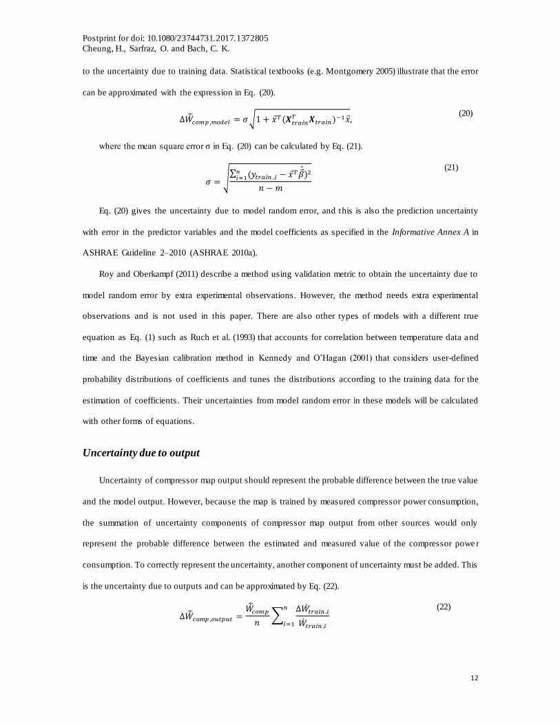
to the uncertainty due to training data. Statistical textbooks (e.g. Montgomery 2005) illustrate that the error

can be approximated with the expression in Eq. (20).

∆��𝑐𝑜𝑚𝑝 ,𝑚𝑜𝑑𝑒𝑙 = 𝜎√1 + 𝑥𝑇(𝑿𝑡𝑟𝑎𝑖𝑛𝑇 𝑿𝑡𝑟𝑎𝑖𝑛)

−1��, (20)

where the mean square error σ in Eq. (20) can be calculated by Eq. (21).

𝜎 = √∑ (𝑦𝑡𝑟𝑎𝑖𝑛 ,𝑖 − 𝑥𝑇 ��

)2𝑛

𝑖=1

𝑛 − 𝑚

(21)

Eq. (20) gives the uncertainty due to model random error, and this is also the prediction uncertainty

with error in the predictor variables and the model coefficients as specified in the Informative Annex A in

ASHRAE Guideline 2–2010 (ASHRAE 2010a).

Roy and Oberkampf (2011) describe a method using validation metric to obtain the uncertainty due to

model random error by extra experimental observations. However, the method needs extra experimental

observations and is not used in this paper. There are also other types of models with a different true

equation as Eq. (1) such as Ruch et al. (1993) that accounts for correlation between temperature data and

time and the Bayesian calibration method in Kennedy and O’Hagan (2001) that considers user-defined

probability distributions of coefficients and tunes the distributions according to the training data for the

estimation of coefficients. Their uncertainties from model random error in these models will be calculated

with other forms of equations.

Uncertainty due to output

Uncertainty of compressor map output should represent the probable difference between the true value

and the model output. However, because the map is trained by measured compressor power consumption,

the summation of uncertainty components of compressor map output from other sources would only

represent the probable difference between the estimated and measured value of the compressor powe r

consumption. To correctly represent the uncertainty, another component of uncertainty must be added. This

is the uncertainty due to outputs and can be approximated by Eq. (22).

Δ��𝑐𝑜𝑚𝑝 ,𝑜𝑢𝑡𝑝𝑢𝑡 =��𝑐𝑜𝑚𝑝

𝑛∑

Δ��𝑡𝑟𝑎𝑖𝑛 ,𝑖

��𝑡𝑟𝑎𝑖𝑛 ,𝑖

𝑛

𝑖=1

(22)



13

Eq. (22) is only applicable to regression models with a normally distributed error term defined in the

same way as Eq. (1). If the error term is defined differently like the error term that is dependent on the input

variables as the one in Kennedy and O’Hagan (2001), then Eq. (22) will not be applicable to the regression

model.


One of the uncertainties to be neglected is uncertainty due to numerical approximation. Roy and

Oberkampf (2011) describe three sources of uncertainty due to numerical approximation: uncertainty due to

discretization, uncertainty due to incomplete iteration and uncertainty due to computational round off that

are all results. Because linear regression does not involve discretization and iterative calculation and the

computation involves 16 significant figures, the uncertainty due to numerical approximation in the

compressor map output can be assumed to be negligible.

Other systematic uncertainties due to conceptual errors in Moffat (1988) are also neglected in this

study. Their magnitude varies dramatically depending on the causes of the error, and examples include

uncertainties due to manufacturing process, system or sensor ageing, and sensor installation location. If it is

caused by a small change of sensor installation location by a model user, it can be negligible. However, if it

is caused by significant ignorance of a model user such as using the compressor suction temperature instead

of compressor suction saturation temperature at the input of the compressor map, they can become more

significant than the uncertainties discussed in this manuscript. Although they can be the largest among all

uncertainties according to Moffat (1988), they are neglected because of the lack of data to estimate them

and they are only significant due to defects or model user ignorance that is too subjective to be quantified

(e.g. application of models under conditions they were not developed for). Uncertainties due to

manufacturing and ageing are created when a map output is used to estimate the power consumption of a

compressor of the same model but in a different setup at a different point of usable lifetime. Because its

quantification can only be done by testing multiple compressors of the same model from a production line

with a well-balanced test matrix and some design of experiments methods, it is assumed to be negligible in

this study for simplicity. However, if a model of compressor is not produced with consistent quality, this

uncertainty will become significant and should be taken into account for correct uncertainty calculation.



14

Likewise, uncertainty due to sensor installation location is created if the inputs are taken from sensors that

are installed differently than the sensors used to collect the training data. While they are often small,

incorrect sensor installation may increase this uncertainty significantly.


Because the uncertainty components are not correlated with each other, the overall standard

uncertainty of the compressor map output can be calculated by the sum of squares of the u ncertainty

components as shown in Eq. (23).

Δ��𝑐𝑜𝑚𝑝 ,𝑠𝑡𝑑 = √Δ��𝑐𝑜𝑚𝑝 ,𝑖𝑛𝑝𝑢𝑡2 + Δ��𝑐𝑜𝑚𝑝 ,𝑡𝑟𝑎𝑖𝑛

2 + Δ��𝑐𝑜𝑚𝑝 ,𝑚𝑜𝑑𝑒𝑙2 + Δ��𝑐𝑜𝑚𝑝 ,𝑜𝑢𝑡𝑝𝑢𝑡

2 (23)


According to ASME PTC 19.1-2013, the standard uncertainty is multiplied by a coverage factor to

illustrate the level of confidence and the accepted practice uses a 95% level of confidence. Because the

number of training data points of the compressor map may be smaller than 60 in this study, the Student’s 𝑡

value of the Student’s 𝑡 distribution is used to calculate the expanded uncertainty as shown in Eq. (24).

Δ��𝑐𝑜𝑚𝑝 ,𝑒𝑥𝑝 = 𝑡𝑛−𝑚,0.95 ⋅ Δ��𝑐𝑜𝑚𝑝 ,𝑠𝑡𝑑 (24)

Case Study

To examine if the method can calculate extrapolation uncertainties of compressor maps appropriately,

compressor calorimeter testing data from Shrestha et al. (2013a) and Shrestha et al. (2013b) are used. The

tests were done to compare the performance of compressors using different refrigerants. Because this

method uses uncertainty of equation of state, only compressor data using refrigerants with well-defined

equations of state are considered in this study. The specifications of the compressors are listed in Table 2.

Table 2: Specification of compressors

Specification Compressor 1

(Shrestha et al. 2013a)

Compressor 2

(Shrestha et al. 2013b)

Compressor type Hermetic scroll

Frequency [Hz] 60

Voltage [V] 208/230



15

Displacement volume [cm3 rev-1] 20.3 51.0

Refrigerant R410A R404A

Rated power consumption [W] 2170 3320

Superheat [K] 11.1

The compressors were tested in calorimeters following the ANSI/ASHRAE Standard 23.1-2010

(ASHRAE 2010b). The uncertainties and locations of the sensors used in the setup are tabulated in Table 3.

Table 3: Uncertainties of sensors used in the setup

Sensors Locations Measurement range Uncertainty

Power energy meter Compressor power

consumption Not available from the

data source ±0.5% of the measured

value

Pressure transmitter 1 Compressor discharge 0 – 5170 kPa ±0.25% full scale

Pressure transmitter 2 Compressor suction 0 – 1380 kPa ±0.25% full scale

Refrigerant mass

flowmeter Condenser outlet

Not available from the

data source

±0.10% of the measured

value

Each compressor was tested under a variety of conditions. To analyze how different sets of training

data affect the size of extrapolation uncertainty, each data set of compressor data is divided into 3 subsets.

The operating conditions of the testing data and the subsets are shown in Figure 2.

(a) Compressor 1 (b) Compressor 2

Figure 2: Operating conditions in compressors tests and the subsets defined for extrapolation uncertainty studies

Figure 2 shows the range of all testing conditions and the subsets for each compressor. Compressor 1

data has 66 available points with compressor discharge dew point temperature ranging from 21.1°C to 60°C

and compressor suction dew point temperature ranging from -12.2°C to 12.8°C. Compressor 2 data has 63

available points with compressor discharge dew point temperature ranging from 21.1°C to 60°C and

compressor suction dew point temperature ranging from -23.3°C to 1.67°C. All Data Set in Figure 2

consists of all testing data points. Set Mid is designed to include data points at the center of the operating

range only, Set Low is designed to include data points with lower dew point temperatures relative to the



16

operating range only, and Set High is designed to include data points with high compressor suction dew

point temperature only.

The choice of training data in Figure 2 is arbitrary in order to demonstrate how the uncertainty

quantifies the effect of extrapolation on the model. In reality, compressor maps are created with at least 14

data points scattered across the entire operating range as shown in Aute et al. (2015), and tech niques in

design of experiments such as Latin-Hypercube-Sampling or D-optimality may be used to choose the

appropriate data points (Montgomery 2005).

The sets of each compressor are used to train their compressor maps separately, and their map outputs

and map output uncertainties of all data points are calculated and compared in the next section.

Although it can be easily observed if a data point lies outside a set and if its corresponding estimation

extrapolates from a map in Figure 2, it is necessary to define a metric for the degree of extrapolation to

analyze the results from all 8 compressor maps. In this case study, the normalized degree of extrapolation is

quantified by Eq. (25).

Normalized degree of extrapolation

= √(𝑇𝑑𝑒𝑤,𝑠𝑢𝑐 − 𝑇𝑑𝑒𝑤,𝑠𝑢𝑐 ,𝑐𝑙𝑜𝑠𝑒

𝑇𝑑𝑒𝑤,𝑠𝑢𝑐 ,𝑡𝑟𝑎𝑖𝑛,𝑚𝑎𝑥 − 𝑇𝑑𝑒𝑤,𝑠𝑢𝑐 ,𝑡𝑟𝑎𝑖𝑛,𝑚𝑖𝑛)

2

+ (𝑇𝑑𝑒𝑤 ,𝑑𝑖𝑠 − 𝑇𝑑𝑒𝑤,𝑑𝑖𝑠,𝑐𝑙𝑜𝑠𝑒

𝑇𝑑𝑒𝑤 ,𝑑𝑖𝑠,𝑡𝑟𝑎𝑖𝑛,𝑚𝑎𝑥 − 𝑇𝑑𝑒𝑤,𝑑𝑖𝑠,𝑡𝑟𝑎𝑖𝑛,𝑚𝑖𝑛)

2

(25)

Eq. (25) shows an equation to calculate the normalized degree of extrapolation which is the

normalization of the shortest distance of an operating point on the boundary of the training data of a map in

Figure 2. While the equation is intuitive to solve for an operating range with a well-defined boundary as

shown in Figure 2, the operating conditions of some compressor maps may not align with the compressor

testing data as regularly as Figure 2 and the compressor operating range may not be as rectangular as

Figure 2 (Winandy et al. 2002; Jähnig et al. 2002). The equation will hence become difficult to be solved in

those situations.

In addition to Eq. (25), a few metrics are needed to summarize the accuracy and uncertainty of the map

results. To summarize the accuracy of the maps, the coefficient of variation from ASHRAE Guideline 14-

2014 (ASHRAE 2014) to assess building model accuracy is used. Its calculation is illustrated in Eq. (26),

and a smaller value implies a more accurate model.



17

𝐶𝑂𝑉 =Sample standard deviation

Mean of the map outputs=𝑛√∑ (��𝑐𝑜𝑚𝑝 ,𝑖 − ��𝑐𝑜𝑚𝑝 )

2𝑛𝑖=1

√𝑛− 1 ∑ ��𝑐𝑜𝑚𝑝 ,𝑖𝑛𝑖=1

(26)

The other metric is relative uncertainty which compares the magnitude of the uncertainty with the map

outputs, and a larger relative uncertainty implies that the value of the map output may deviate more with its

true value. Relative uncertainty is calculated per Eq. (27).

Relative overall uncertainty =Δ��𝑐𝑜𝑚𝑝 ,𝑒𝑥𝑝

��𝑐𝑜𝑚𝑝

(27)

Similarly, a relative uncertainty of an uncertainty component as calculated in Eq. (28) is used.

Relative uncertainty of an uncertainty component =Δ��𝑐𝑜𝑚𝑝 ,𝑑𝑒𝑐𝑜𝑢𝑝𝑙𝑒𝑑

��𝑐𝑜𝑚𝑝

(28)

where Δ��𝑐𝑜𝑚𝑝 ,𝑑𝑒𝑐𝑜𝑢𝑝𝑙𝑒𝑑 in Eq. (28) can be any uncertainty component.

Results and Discussion

Accuracy of maps and example application of the method

To examine the accuracy of the maps within the training data points, the coefficients of variation of

different maps calculated from their estimation over their training data points are tabulated in Table 4.

Table 4: Coefficients of variation over their training data points for all trained

compressor maps

Compressor 1 Coefficient

of variation

Number of

training

data points


of variation

Number of

training data

points

Map from All Data Set

0.0021 66 Map from All Data

Set 0.0013 63

Map from Set Mid 0.0004 16 Map from Set Mid 0.0002 16

Map from Set Low 0.0021 39 Map from Set Low 0.0012 39

Map from Set High 0.0010 25 Map from Set High 0.0007 25

Table 4 shows that the coefficients of variation for all maps over their training data points are smaller

than 1%, and hence the maps should be very accurate over the range of their training data points. However,

the maps may not be accurate when extrapolated. To illustrate the potential inaccuracy, the estimated power

consumption of map from Set High of both compressors is plotted in Figure 3.



18

(a) Compressor 1

(b) Compressor 2

Figure 3: Comparison between measured and estimated power consumption for the map from Set High of both

compressors with overall expanded uncertainty of map outputs

Figure 3 shows that maps from Set High of both compressor’s maps are able to estimate the power

consumption at the conditions of training data points correctly. However, when the uncertainty of the

estimation is high at conditions different from the training data, the map from Set High of compressor 1

cannot predict the power consumption accurately while the map from Set High of compressor 2 can predict

accurately.

Figure 3 also demonstrates an example application of the uncertainty calculation method. In Figure

3(a), some data points are estimated with small uncertainty values and high accuracy despite their absence

in the training data. This shows that the estimation of power consumption at these data points can be trusted

and used for other purposes. However, the ones with large uncertainties are also associated with high

inaccuracy, indicating that they cannot be trusted unless training data at conditions other that the Set High

in Figure 2 are introduced. Although the rule is not well followed by the results in Figure 3(b), this is true

for other choices of sets as shown in the Appendix B, indicating that the uncertainty calculation method can

be used to identify if the estimation of power consumption under certain condition is reliable and can be

trusted according to its training data conditions.

Change of overall expanded uncertainty with degree of extrapolation



19

In order to analyze if the overall expanded uncertainty can represent the degree of extrapolation at a

data point, the normalized degrees of extrapolation from Eq. (25) is plotted with the relative overall

uncertainty for all maps defined in Figure 2 as shown in Figure 4.

(a) Compressor 1

(b) Compressor 2

Figure 4: Change of relative overall expanded uncertainty with normalized degree of extrapolation for all maps

Figure 4 shows that for maps in both compressors, the relative overall uncertainty depends strongly on

the normalized degree of extrapolation and increases with an increase in the normalized degree of

extrapolation. A similar behavior was observed in Cheung and Bach (2015) for an increase in extrapolation,

there expressed in terms of minimum °C distance to nearest training data point.

Change of overall expanded uncertainty with map accuracy

Figure 5 is plotted to understand how the uncertainty changes with map accuracy.



20

(a) Compressor 1

(b) Compressor 2

Figure 5: Change of relative overall expanded uncertainty with map accuracy in all maps

Figure 5(a) for compressor 1 shows that the accurate maps have low relative uncertainty and

uncertainty increases with an increase in map inaccuracy as found in Cheung and Bach (2015). For

compressor 2, Figure 5(b) shows that maps from Set Mid and Low show the similar behavior as maps in

compressor 1, however, map from Set High has almost same accuracy for different values of overall

relative uncertainty. This shows that the map accuracy does not have a definite relationship with relative

overall uncertainty and maps that are accurate at extrapolation may still yield large relative overall

uncertainty.

Figure 5 also shows an approach for a user to justify the use of an extrapolation scenario based on the

overall expanded uncertainty. A user can use the maximum relative overall expanded uncertainties at the

training data points to set a threshold, and reject any extrapolation cases with overall expanded uncertainty

is higher than that threshold. For example, the maximum relative overall expanded uncertainty at the

training data points of the map generated from Set Mid of Compressor 2 is 0.0313. If a user uses the map to

estimate the power consumption of all Compressor 2 data points in Figure 2(b) and rejects cases with

relative overall uncertainties higher than 0.0313, the user can keep 19 out of 47 ext rapolation cases with an

average map accuracy at 0.75% among the accepted extrapolation cases and achieves a good accuracy

relative to the average map accuracy at 0.44% for the training data points. If a user can tolerate higher

inaccuracy at the extrapolation cases, a threshold higher than the maxmium value can be set to match the

needs of different users .



21

Change of uncertainty components with extrapolation

To find the uncertainty component that increases with extrapolation, the squares of uncertainty

components of map outputs in all maps are plotted with the normalized degree of extrapolation as shown in

Figure 6.

(a) Compressor 1

(b) Compressor 2

Figure 6: Change of uncertainty components in map outputs with normalized degree of extrapolation in all maps

The uncertainty components in Figure 6 are squared because uncertainty due to correlated training data

can be complex. It shows that the uncertainty due to model random error increases as normalized degree of

extrapolation increases. This shows that the uncertainty due to model random error is responsible for the

increase of the uncertainty as the compressor maps extrapolate. The significance of other uncertainty

components remains the same with extrapolation, and it can be listed in a descending order as the



22

uncertainty due to training data, the low-order uncertainty due to inputs, the uncertainty due to output and

the high-order uncertainty due to inputs, which is insignificant and can be neglected.

The results in Figure 6 also show that the calculation method is different from that in Aute et al. (2015)

because their method, as shown by Coleman and Steele (2009) to be equivalent to the uncertainty due to

inputs and uncertainty due to training data, would under-predict the uncertainty when the degree of

extrapolation is higher than 1.0 and the uncertainty due to model random error is significant. Hence the

method presented in this paper will lead to better predictions than the method presented by Aute et al.

(2015) when extrapolation occurs.

One major difference between Figure 6 and the conclusion in Cheung and Bach (2015) is that the

uncertainty due to training data in Figure 6 does not increase with extrapolation unlike the conclusion in

Cheung and Bach (2015). The reason is that Cheung and Bach (2015) does not include the uncertainty due

to correlated training data as calculated in Eq. (18).

(a) Compressor 1

(b) Compressor 2

Figure 7: Change of components of uncertainty due to training data in map outputs with normalized degree of

extrapolation in all maps

Figure 7 shows that the uncertainty due to uncorrelated training data increases with extrapolation as

found in Cheung and Bach (2015). However, the correlation of training data that is decreasing with

extrapolation in Figure 7 is not considered in Cheung and Bach (2015). Unlike other uncertainty

components, the square of the uncertainty due to correlated training data can be negative because all of its

terms in Eq. (18) are not restricted to be positive. As maps extrapolate, the reduction of the uncertainty of



23

correlated data partially offsets the increase of the uncertainties of the uncorrelated data, resulting in

relatively constant uncertainty due to training data in Figure 6. Hence the uncertainty due to correlated

training data is not negligible if uncertainty due to training data is calculated.

Change of uncertainty due to training data with choice of training data

To examine the choices of training data affect uncertainty due to training data, the relative

uncertainties from training data of different maps are compared with each other as shown in Figure 8.

(a) Compressor 1

(b) Compressor 2

Figure 8: Comparison of uncertainties due to training data from different maps at all operating conditions

Figure 8 shows that the uncertainties due to training data from different maps are not significantly

different for both compressors and all of them decrease with higher compressor power consumption. This

shows that the magnitude of uncertainty due to training data does not depend on the choice of training data

of compressor maps but on other factors such as the input conditions of the compressor or the magnitude of

the training data.

Application of the method to other types of compressor map outputs

The 10-coefficient map in Eq. (6) is not only applied to power consumption estimation but also to

other variables of compressors such as refrigerant mass flow rate and cooling capacity of a vapor

compression system. To examine if the uncertainty calculation method is applicable to other types of

outputs, the method is applied to the refrigerant mass flow rates measured in Shrestha et al. (2013a) and

Shrestha et al. (2013b) in a similar manner, and the results are shown in Figure 9 and Figure 10.



24

(a) Compressor 1

(b) Compressor 2


estimating refrigerant mass flow rates

(a) Compressor 1

(b) Compressor 2

Figure 10: Change of overall expanded uncertainty with map deviation in all maps estimating refrigerant mass flow

rate

Figure 9 and Figure 10 show similar results as the power consumption compressor maps. Extrapolation

cases show high overall expanded uncertainties and high overall expanded uncertainties refer to cases with

poor map accuracy. Hence the method is also applicable to other types of compressor maps.

Conclusions and future work

In summary, a method to calculate the uncertainty of compressor map output is developed. The method

considers the effects of the mathematical structure of the map, the choice of training data, the uncertainties



25

of the training data, the uncertainties of related measurement devices, and the equation of state of

refrigerants. It calculates the map output uncertainty by 4 major components and is tested with case studies

by measurement data from 2 compressors. The results show that high -order uncertainties are negligible

despite the cubic structure of the map. With little extrapolation, the uncertainty due to training data is the

most significant uncertainty component though uncertainty due to inputs is the most common one to be

calculated. When the maps extrapolate, their uncertainties due to model random error increases with map

extrapolation and may become larger than other components. Although the uncertainty due to model

random error is a good indicator of extrapolation inaccuracy, extrapolation may not necessarily imply

inaccuracy of the maps and hence the method occasionally exaggerates the inaccuracy problem due to

extrapolation, which would require future work for improvement. By calculating the overall expanded

uncertainty of a compressor map and defining an accuracy threshold, a user can decide if an extrapolation

case is acceptable. The method allows the quantification of the extrapolation effect of the compressor

model and helps to verify thermal system models that simulate off-design conditions (ASME 2006;

Coleman and Steele 2009). Such conditions occur in applications that include faulted vapor compression

systems, cold climate heat pumps, air conditioner start-up and shutdown processes, pump down operation

of refrigeration systems, etc.

In the future, the uncertainty calculation framework in this paper will be used to compare the

extrapolation capability of different types of compressor models to examine if models using more physical

rules are more reliable in extrapolation cases. The framework will also be used to develop a general rule of

thumb to determine when an extrapolation case is acceptable for different types of compressor models and

compressors.

Nomenclature

𝛽 Coefficient of a 10-coefficient map [unit varies]

COV Coefficient of variation [dimensionless]

𝜀 Error between true value and estimation of a variable from a linear model [unit varies]

Δ Uncertainty of a variable [unit varies]

m Number of coefficients of 10-coefficient map [dimensionless]

n Number of training data points [dimensionless] P Pressure [kPa]

r Relative uncertainty [dimensionless]

𝜎 Mean square error [W]

T Temperature [K]

𝑡𝑛−𝑚,0.95 Student’s 𝑡 value for a 95% confidence interval of estimates from equations with n training data



26

points and m coefficients

�� Power consumption [W]

x Independent variable [unit varies] X Matrix of independent variables [unit varies]

y Dependent variable [unit varies]

Accent

Vectorized

Estimated

Subscript

close Closest operating point on the boundary of the training data of a compressor map

comp Compressor

corr Correlated

dew Dew point dis Discharge

EOS Equation of state

exp Expanded

full Full-scale

high High-order i ith entry of a variable or coefficient

input Uncertainty due to input

j jth entry of a variable

low Low-order max Maximum

mea Measured

min Minimum

model Uncertainty due to model random error

output Uncertainty due to output P Pressure transducer

std Standard

suc Suction

train Training data

true True model of linear regression uncorr Uncorrelated

References

AHRI. (2004). ANSI/AHRI Standard 540: 2004 Standard for Performance Rating of Positive Displacement

Refrigerant Compressors and Compressor Units. Arlington: Air-Conditioning, Heating, and

Refrigeration Institute.

AHRI. (2016). Final Low-GWP AREP Test Reports. Retrieved September 21, 2016, from

http://www.ahrinet.org/Resources/Research/AHRI-Low-GWP-Alternative-Refrigerants-

Evaluation-Program/Reports-by-Category.aspx#Comp

ASHRAE. (2010a). ANSI/ASHRAE Guideline 2-2010: Engineering Analysis of Experimental Data.

Atlanta: American Society of Heating, Refrigerating and Air-Conditioning Engineers, Inc.

ASHRAE. (2010b). ANSI/ASHRAE Standard 23.1-2010: Methods of Testing for Rating the Performance

of Positive Displacement Refrigerant Compressors and Condensing Units That Operate at

Subcritical Temperatures. Atlanta: American Society of Heating, Refrigerating and Air-

Conditioning Engineers, Inc.

ASHRAE. (2014). ASHRAE Guideline 14-2014: Measurement of Energy, Demand, and Water Savings.

Atlanta: American Society of Heating, Refrigerating and Air-Conditioning Engineers, Inc.

ASME. (2006). ASME V&V 10-2006 Guide for Verification and Validation in Computational Solid

Mechanics. New York: American Society of Mechanical Engineers.



27

ASME. (2013). ASME PTC 19.1-2013: Test Uncertainty Performance Test Codes. New York: American

Society of Mechanical Engineers.

Aute, V., Martin, C., & Radermacher, R. (2015). A Study of Methods to Represent Compressor

Performance Data over an Operating Envelope Based on a Finite Set of Test Data (No. 8013).

College Park, MD: Air-Conditioning, Heating, and Refrigeration Institute.

Bach, C. K., & Cheung, H. (2016). Mapping of Vapor Injected Compressor with Consideration of

Extrapolation Uncertainty. ASHRAE Orlando 2016 Conference Paper. Orlando: American Society

of Heating, Refrigerating and Air-Conditioning Engineers, Inc.

Bach, C. K., Groll, E. A., & Braun, J. E. (2016). Dual port vapor injected compression: In -system testing

versus test stand testing, and mapping of results. Renewable Energy, 819-833.

Bell, I. H., Lemort, V., Groll, E. A., Braun, J. E., King, G. B., & Horton, W. T. (2012). Liquid-flooded

compression and expansion in scroll machines – Part I: Model development. International Journal

of Refrigeration, 35(7), 1878–1889.

Bell, I. H., Wronski, J., Quoilin, S., & Lemort, V. (2014). Pure and Pseudo-pure Fluid Thermophysical

Property Evaluation and the Open-Source Thermophysical Property Library CoolProp. Industrial

and Engineering Chemistry Research, 53(6), 2498-2508.

Caskey, S., Kultgen, D., Groll, E., Hutzel, W., & Menzi, T. (2012). Simulation of an Air-Source Heat

Pump with Two-Stage Compression and Economizing for Cold Climates. International

Refrigeration and Air Conditioning Conference.

CEN. (2013). EN 12900: Refrigerant Compressors - Rating Conditions, Tolerances and Presentation of

Manufacturer's Performance Data. Brussels: European Committee for Standardisation.

Cheung, H., & Bach, C. K. (2015). Prediction of Uncertainty of 10-coefficient Compressor Maps for

Extreme Operating Conditions. IOP Conference Series: Materials Science and Engineering .

90(1), p. 012078. IOP Publishing.

Cheung, H., & Braun, J. E. (2013). Simulation of fault impacts for vapor compression systems by inverse

modeling. Part II: System modeling and validation. HVAC&R Research, 19(7), 907–921.

Coleman, H. W., & Steele, W. G. (2009). Experimentation, Validation, and Uncertainty Analysis for

Engineers (3 edition). Hoboken, N.J: Wiley.

Dardenne, L., Fraccari, E., Maggioni, A., Molinaroli, L., Proserpio, L., & Winandy., E. (2015). Semi-

Empirical Modelling of a Variable Speed Scroll Compressor with Vapour Injection. International

Journal of Refrigeration, 54, 76-87.

Ding, G. (2007). Recent developments in simulation techniques for vapour-compression refrigeration

systems. International Journal of Refrigeration , 30(7), 1119–1133.

Gall, J., Fisher, D. E., Corti, G., Marelli, S., & Cremaschi, L. (2015). Modeling of R-410A variable

capacity compressor with Modelica and experimental validation. International Journal of

Refrigeration, 58, 90-109.

Heo, J., Yun, R., & Kim, Y. (2013). Simulations on the performance of a vapor-injection heat pump for

different cylinder volume ratios of a twin rotary compressor. International Journal of

Refrigeration, 36(3), 730–744.

Ibsaine, R., Joffroy, J.-M., & Stouffs, P. (2016). Modelling of a new thermal compressor for supercritical

CO2 heat pump. Energy.

Jähnig, D. I., Reindl, D. T., & Klein, S. A. (2000). A Semi-Empirical Method for Representing Domestic

Refrigerator/Freezer Compressor Calorimeter Test Data. ASHRAE Transactions, 106(2), 122–130.

JCGM. (2008). JCGM 100:2008: Evaluation of Measurement Data – Guide to the Expression of

Uncertainty in Measurement. Joint Committee for Guides in Metrology.

Kamei, A., Beyerlein, S. W., & Jacobsen, R. T. (1995). Application of Nonlinear Regression in the

Development of a Wide Range Formation for HCFC-22. International Journal of Thermophysics,

16(5), 1155 – 1164.

Kennedy, M. C., & O’Hagan, A. (2001). Bayesian Calibration of Computer Models. Journal of the Royal

Statistical Society: Series B (Statistical Methodology), 63(3), 425 - 464.

Lemmon, E. W. (2003). Pseudo-Pure Fluid Equations of State for the Refrigerant Blends R-410A, R-404A,

R-507C, and R-407C. International Journal of Thermophysics, 24(4), 991 - 1006.

Li, W. (2012). Simplified steady-state modeling for hermetic compressors with focus on extrapolation.

International Journal of Refrigeration , 35(6), 1722–1733.

Moffat, R. J. (1988). Describing the uncertainties in experimental results. Experimental Thermal and Fluid

Science, 1(1), 3–17.



28

Molinaroli, L., Joppolo, C. M., & De Antonellis, S. (2017). A Semi-Empirical Model for Hermetic Rolling

Piston Compressors. International Journal of Refrigeration , doi:10.1016/j.ijrefrig.2017.04.015.

Montgomery, D. (2005). Design and Analysis of Experiments, 6th Edition. Jon Wiley & Sons .

Navarro, E., Redón, A., Gonzálvez-Macia, J., Martinez-Galvan, I., & Corberán, J. (2013). Characterization

of a Vapor Injection Scroll Compressor as a Function of Low, Intermediate and High Pressures

and Temperature Conditions. International Journal of Refrigeration , 36(7), 1821–1829.

Park, Y. C., Kim, Y. C., & Min, M.-K. (2001). Performance analysis on a multi-type inverter air

conditioner. Energy Conversion and Management, 42(13), 1607–1621.

Rasmussen, B. P. (2012). Dynamic modeling for vapor compression systems —Part I: Literature review.

HVAC&R Research, 18(5), 934–955.

Rice, C. K., & Jackson, W. L. (2005). DOE/ORNL Heat Pump Design Model on the Web, Mark VII

Version. Retrieved September 21, 2016, from http://web.ornl.gov/~wlj/hpdm/MarkVII.shtml

Roy, C. J., & Oberkampf, L. W. (2011). A comprehensive framework for verification, validation, and

uncertainty quantification in scientific computing. Computer Methods in Applied Mechanics and

Engineering, 200, 2131 – 2144.

Ruch, D. K., & Claridge, D. E. (1993). A Development and Comparison of NAC estimates for Linear and

Change-point Energy Models for Commercial Buildings. Energy and Buildings, 20, 87 – 95.

Shao, S., Shi, W., Li., X., & H., C. (2004). Performance representation of variable-speed compressor for

inverter air conditioners based on experimental data. International Journal of Refrigeration , 27,

805 - 815.

Shen, B., Braun, J. E., & Groll, E. A. (2009). Improved methodologies for simulating unitary air

conditioners at off-design conditions. International Journal of Refrigeration , 32(7), 1837–1849.

Shrestha, S., Mahderekal, I., Sharma, V., & Abdelaziz, O. (2013a). Compressor Calorimeter Test of R-

410A Alternatives R-32, DR-5, And L-41a. Oak Ridge: Oak Ridge National Laboratory.

Shrestha, S., Sharma, V., & Abdelaziz, O. (2013b). Compressor Calorimeter Test of R-404A Alternatives

ARM-31a, D2Y-65, L-40, and R32+ R-134a Mixture using a Scroll Compressor. Oak Ridge: Oak

Ridge National Laboratory.

Thorade, M., & Saadat., A. (2013). Partial derivatives of thermodynamic state properties for dynamic

simulation. Environmental Earth Sciences, 70(8), 3497-3503.

Wang, S., Wang, J., & Burnett, J. (2000). Mechanistic model of centrifugal chillers for HVAC system

dynamics simulation. Building Services Engineering Research and Technology , 21(2), 73–83.

Wang, B., Shi, W., Li, X., & Yan., Q. (2008). Numerical Research on the Scroll Compressor with

Refrigeration Injection. Applied Thermal Engineering , 28, 440-449.

Winandy, E., O., C. S., & Lebrun, J. (2002). Experimental Analysis and Simplified Modelling of a

Hermetic Scroll Refrigeration Compressor. Applied Thermal Engineering, 220, 107-120.

Zakula, T., Gayeski, N. T., Armstrong, P. R., & Norford, L. K. (2011). Variable-speed heat pump model

for a wide range of cooling conditions and loads. HVAC&R Research, 17(5), 670–691.



29

Appendix A Analytical Calculation of Partial Derivatives with Respect to Training

Data Points in Eq. (17) and (18)

This appendix describes the analytical derivation of the formula to calculate the partial derivatives of

coefficients with respect to training data observations in Eq. (17) and (18).

Calculating partial derivatives of coefficients with respect to training data observations

of compressor power consumption

To calculate the partial derivative, the product rule can be used to split the derivative of coefficients as

Eq. (29).

𝜕𝛽

𝜕��𝑐𝑜𝑚𝑝 ,𝑡𝑟𝑎𝑖𝑛,𝑗

=𝜕𝛽

𝜕��𝑡𝑟𝑎𝑖𝑛


𝜕��𝑐𝑜𝑚𝑝 ,𝑡𝑟𝑎𝑖𝑛 ,𝑗

(29)

where j means the jth

entry in the vector ��𝑡𝑟𝑎𝑖𝑛

The first partial derivative in Eq. (29) can be calculated from the estimation equation of the

coefficients as Eq. (30).

𝜕𝛽


= (𝑿𝒕𝒓𝒂𝒊𝒏𝑻 𝑿𝒕𝒓𝒂𝒊𝒏)

−1𝑿𝒕𝒓𝒂𝒊𝒏𝑻

(30)

The second derivative in Eq. (29) is a zero vector except the jth

entry which is one, and 𝜕𝛽𝑖

𝜕��𝑐𝑜𝑚𝑝,𝑡𝑟𝑎𝑖𝑛,𝑗 in

Eq. (17) and (18) is the ith

entry in the vector 𝜕��

𝜕��𝑐𝑜𝑚𝑝,𝑡𝑟𝑎𝑖𝑛,𝑗.

Calculating partial derivative of coefficients with respect to training data observations

of compressor suction and discharge dew point temperature

By matrix calculus, the partial derivative of coefficients with respect to a compressor suction dew point

temperature in the training data can be obtained by differentiating Eq. (3) into multiple parts as Eq. (31) to

(34).

𝜕𝛽

𝜕𝑇𝑑𝑒𝑤 ,𝑠𝑢𝑐,𝑗

= [𝜕(𝑿𝒕𝒓𝒂𝒊𝒏

𝑻 𝑿𝒕𝒓𝒂𝒊𝒏)−1


𝑿𝒕𝒓𝒂𝒊𝒏𝑻 + (𝑿𝒕𝒓𝒂𝒊𝒏


𝜕𝑿𝒕𝒓𝒂𝒊𝒏𝑻


] ��𝑐𝑜𝑚𝑝 ,𝑡𝑟𝑎𝑖𝑛 (31)

𝜕(𝑿𝒕𝒓𝒂𝒊𝒏𝑻 𝑿𝒕𝒓𝒂𝒊𝒏)

−1


= −(𝑿𝒕𝒓𝒂𝒊𝒏𝑻 𝑿𝒕𝒓𝒂𝒊𝒏)

−1𝜕(𝑿𝒕𝒓𝒂𝒊𝒏

𝑻 𝑿𝒕𝒓𝒂𝒊𝒏)

𝜕𝑇𝑑𝑒𝑤,𝑠𝑢𝑐 ,𝑗(𝑿𝒕𝒓𝒂𝒊𝒏


(32)



30

𝜕(𝑿𝒕𝒓𝒂𝒊𝒏𝑻 𝑿𝒕𝒓𝒂𝒊𝒏)

𝜕𝑇𝑑𝑒𝑤,𝑠𝑢𝑐,𝑗=



𝑿𝒕𝒓𝒂𝒊𝒏 +𝑿𝒕𝒓𝒂𝒊𝒏𝑻

𝜕𝑿𝒕𝒓𝒂𝒊𝒏


(33)


𝜕𝑇𝑑𝑒𝑤,𝑠𝑢𝑐 ,𝑗= (


𝜕𝑇𝑑𝑒𝑤,𝑠𝑢𝑐,𝑗)

𝑇

(34)


𝜕𝑇𝑑𝑒𝑤,𝑠𝑢𝑐,𝑗 is a matrix with zero values except its j

th row as shown in Eq. (35).



=

[

0 ⋯ 0⋮

0 1 0 2𝑇𝑑𝑒𝑤 ,𝑠𝑢𝑐,𝑗 𝑇𝑑𝑒𝑤,𝑑𝑖𝑠,𝑗 0 3𝑇𝑑𝑒𝑤 ,𝑠𝑢𝑐,𝑗2 2𝑇𝑑𝑒𝑤,𝑠𝑢𝑐 ,𝑗𝑇𝑑𝑒𝑤,𝑑𝑖𝑠,𝑗 𝑇𝑑𝑒𝑤,𝑑𝑖𝑠,𝑗

2 0

⋮0 ⋯ 0 ]

(35)

The partial derivative of the ith

coefficient with respect to the jth

compressor suction dew point

temperature in the training data can be obtained by selecting the ith

entry in the partial derivative of the

coefficient vector in Eq. (31).

The partial derivative of the coefficient vector with respect to compressor discharge dew point

temperature in training data can be obtained by substituting the compressor suction dew point temperature

from Eq. (31) to (34) by compressor discharge dew point temperature and calculating 𝜕𝑿𝒕𝒓𝒂𝒊𝒏

𝜕𝑇𝑑𝑒𝑤,𝑑𝑖𝑠,𝑗 by Eq. (36).


𝜕𝑇𝑑𝑒𝑤,𝑑𝑖𝑠,𝑗=

[

0 ⋯ 0⋮

0 0 1 0 2𝑇𝑑𝑒𝑤,𝑑𝑖𝑠,𝑗 𝑇𝑑𝑒𝑤,𝑑𝑖𝑠,𝑗 0 𝑇𝑑𝑒𝑤,𝑠𝑢𝑐,𝑗2 2𝑇𝑑𝑒𝑤,𝑠𝑢𝑐 ,𝑗𝑇𝑑𝑒𝑤,𝑑𝑖𝑠,𝑗 3𝑇𝑑𝑒𝑤,𝑑𝑖𝑠,𝑗

2

⋮0 ⋯ 0 ]

(36)



31

Appendix B Parity Plots of Measured and Estimated Power Consumption of

Different Compressor Maps Calibrated by Different Sets of Training Data

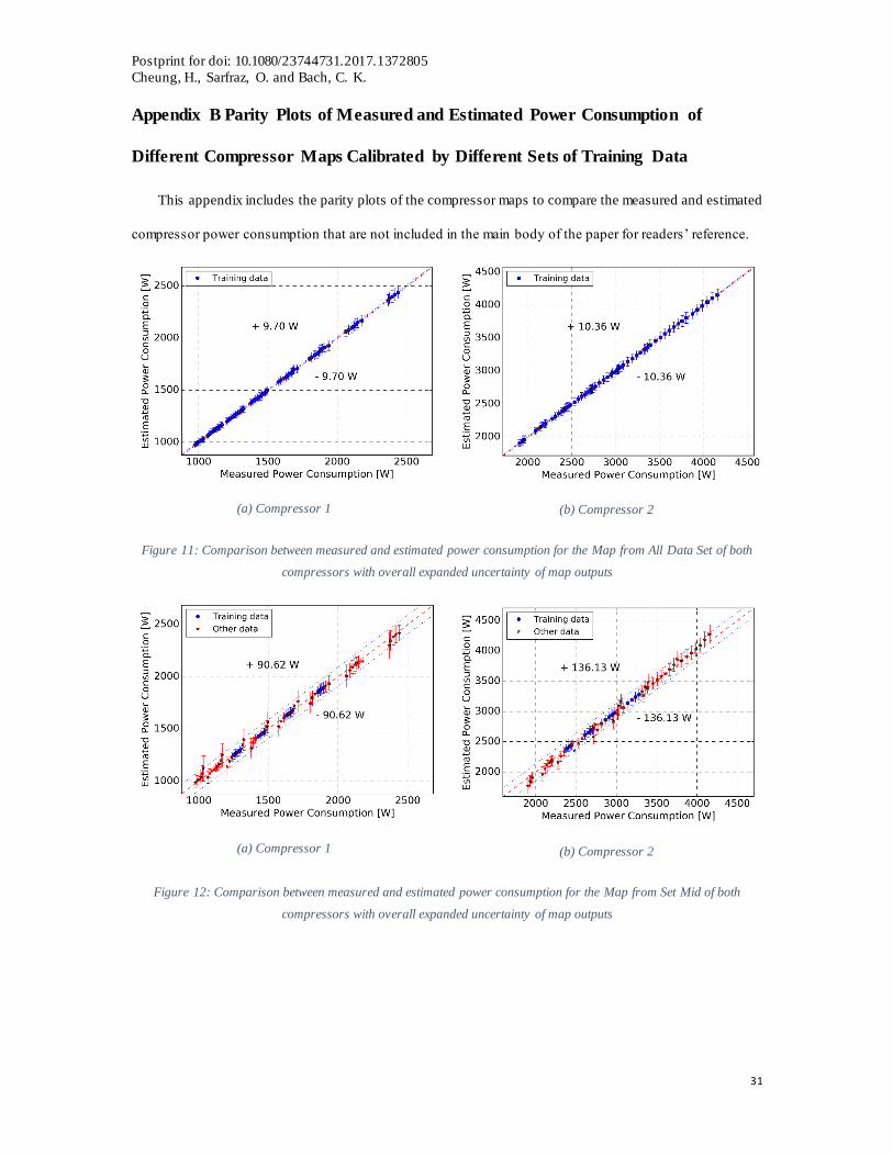
This appendix includes the parity plots of the compressor maps to compare the measured and estimated

compressor power consumption that are not included in the main body of the paper for readers’ reference.

(a) Compressor 1

(b) Compressor 2

Figure 11: Comparison between measured and estimated power consumption for the Map from All Data Set of both


(a) Compressor 1

(b) Compressor 2

Figure 12: Comparison between measured and estimated power consumption for the Map from Set Mid of both




32

(a) Compressor 1

(b) Compressor 2

Figure 13: Comparison between measured and estimated power consumption for the Map from Set Low of both




33

Figures

Figure 1: Flowchart of uncertainty propagation to the compressor map output

(a) Compressor 1 (b) Compressor 2

Figure 2: Operating conditions in compressors tests and the subsets defined for extrapolation uncertainty studies






Uncertainty due to outputs

Uncertainty of power



Uncertainty due to model random

error




temperature for map inputs


measurement for map inputs


temperature in training data

20

25

30

35

40

45

50

55

60

65

-15 -5 5 15

De

wp

oin

t at

co

mp

ress

or

dis

char

ge [

°C]

Dewpoint at compressor suction [°C]

Operating Range

All Data

Map 1

Map 2

Map 3

20

25

30

35

40

45

50

55

60

65

-25 -15 -5 5

De

wp

oin

t at

co

mp

ress

or

dis

char

ge [

°C]

Dewpoint at compressor suction [°C]

OperatingRange

All Data Set

Set Mid

Set Low

Set High



34

(a) Compressor 1

(b) Compressor 2

Figure 3: Comparison between measured and estimated power consumption for the map from Set High of both


(a) Compressor 1

(b) Compressor 2




35

(a) Compressor 1

(b) Compressor 2

Figure 5: Change of relative overall expanded uncertainty with map accuracy in all maps



36

(a) Compressor 1

(b) Compressor 2

Figure 6: Change of uncertainty components in map outputs with normalized degree of extrapolation in all maps



37

(a) Compressor 1

(b) Compressor 2

Figure 7: Change of components of uncertainty due to training data in map outputs with normalized degree of

extrapolation in all maps

(a) Compressor 1

(b) Compressor 2

Figure 8: Comparison of uncertainties due to training data from different maps at all operating conditions



38

(a) Compressor 1

(b) Compressor 2


estimating refrigerant mass flow rates

(a) Compressor 1

(b) Compressor 2

Figure 10: Change of overall expanded uncertainty with map deviation in all maps estimating refrigerant mass flow

rate



39

(a) Compressor 1

(b) Compressor 2

Figure 11: Comparison between measured and estimated power consumption for the Map from All Data Set of both


(a) Compressor 1

(b) Compressor 2

Figure 12: Comparison between measured and estimated power consumption for the Map from Set Mid of both




40

(a) Compressor 1

(b) Compressor 2

Figure 13: Comparison between measured and estimated power consumption for the Map from Set Low of both




41

Tables

Table 1: Uncertainty of equations of states of different

refrigerant

Refrigerant Uncertainty Literature

R22 0.2% of the dew point pressure Kamei et al. (1995)



Table 2: Specification of compressors

Specification Compressor 1

(Shrestha et al. 2013a)

Compressor 2

(Shrestha et al. 2013b)

Compressor type Hermetic scroll

Frequency [Hz] 60

Voltage [V] 208/230

Displacement volume [cm3 rev-1] 20.3 51.0

Refrigerant R410A R404A

Rated power consumption [W] 2170 3320

Superheat [K] 11.1

Table 3: Uncertainties of sensors used in the setup

Sensors Locations Measurement range Uncertainty

Power energy meter Compressor power

consumption


data source


value

Pressure transmitter 1 Compressor discharge 0 – 5170 kPa ±0.25% full scale

Pressure transmitter 2 Compressor suction 0 – 1380 kPa ±0.25% full scale

Refrigerant mass

flowmeter Condenser outlet


data source


value

Table 5: Coefficients of variation over their training data points for all trained

compressor maps


of variation

Number of

training

data points


of variation

Number of

training data

points

Map from All Data

Set 0.0021 66

Map from All Data

Set 0.0013 63

Map from Set Mid 0.0004 16 Map from Set Mid 0.0002 16

Map from Set Low 0.0021 39 Map from Set Low 0.0012 39

Map from Set High 0.0010 25 Map from Set High 0.0007 25

Documents

A Method to Calculate Uncertainty of Empirical Compressor ... · measurements of compressor suction and discharge pressure in calorimeter tests and are commonly used by compressor