Contents lists available at ScienceDirect

Fuel

journal homepage: www.elsevier.com/locate/fuel

Full Length Article

A method for retrieving char oxidation kinetic data from reacting particletrajectories in a novel test facility

Wojciech P. Adamczyka, Ryszard A. Białeckia, Mario Ditarantob, Nils Erland L. Haugenb,Anna Katelbach-Woźniaka, Adam Klimaneka,⁎, Sławomir Sładeka, Andrzej Szlęka, Gabriel Węcelaa Institute of Thermal Technology, Silesian University of Technology, Konarskiego 22, 44-100 Gliwice, Polandb SINTEF Energi A.S., Sem Saelands vei 11, 7034 Trondheim, Norway

G R A P H I C A L A B S T R A C T

A R T I C L E I N F O

Keywords:Coal combustion kineticsCombustion ratesCionKinetic dataInverse methodUncertainty quantification

A B S T R A C T

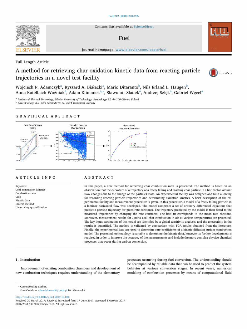
In this paper, a new method for retrieving char combustion rates is presented. The method is based on anobservation that the curvature of a trajectory of a freely falling and reacting char particle in a horizontal laminarflow changes due to the change of the particles mass. An experimental facility was designed and built allowingfor recording reacting particle trajectories and determining oxidation kinetics. A brief description of the ex-perimental facility and measurement procedure is given. In this procedure, a model of a freely falling particle ina laminar horizontal flow was developed. The model comprises a set of ordinary differential equations thatpredict a particle trajectory for given rate constants. The trajectory predicted by the model is then fitted to themeasured trajectories by changing the rate constants. The best fit corresponds to the mean rate constant.Moreover, measurement results for Janina coal char combustion in air at various temperatures are presented.The key input parameters of the model are identified by a global sensitivity analysis, and the uncertainty in theresults is quantified. The method is validated by comparison with TGA results obtained from the literature.Finally, the experimental data are used to determine rate coefficients of a kinetic-diffusion surface combustionmodel. The presented methodology is suitable to determine the kinetic data, however its further development isrequired in order to improve the accuracy of the measurements and include the more complex physico-chemicalprocesses that occur during carbon conversion.

1. Introduction

Improvement of existing combustion chambers and development ofnew combustion techniques requires understanding of the elementary

processes occurring during fuel conversion. The understanding shouldbe accompanied by reliable data that can be used to predict the systembehavior at various conversion stages. In recent years, numericalmodeling of combustion processes by means of computational fluid

http://dx.doi.org/10.1016/j.fuel.2017.10.020Received 20 March 2017; Received in revised form 17 June 2017; Accepted 5 October 2017

⁎ Corresponding author.E-mail address: adam.klimanek@polsl.pl (A. Klimanek).

Fuel 212 (2018) 240–255

0016-2361/ © 2017 Elsevier Ltd. All rights reserved.

MARK

dynamics (CFD) tools became an integral part of the design and opti-mization processes. The models used in the simulations require closureapproximations, which are based on experimental data. In order toimprove the predicted system behavior, the quality of the data shouldbe high and the closure models themselves should be fast, robust andaccurate. Kinetic parameters of drying, devolatilization and char gasi-fication/combustion, together with ignition characteristics, are crucialelements of simulations of combustion processes. It should be stressedthat the experimental data, from which the kinetic parameters are ob-tained, should be determined at relevant process conditions.Specifically the temperature, the heating rate, the thermal history, thepressure and the atmosphere are of importance [1,2]. Drop tube fur-naces (DTF) are already standard devices used to retrieve such data. Inrecent years, many studies were devoted to characterization of solidfuels. These include ignition characteristics [3–7], kinetic parameters ofdevolatilization [1,2,8,9], combustion [10–13] and gasification[14–18] processes. The conditions achievable in drop tube reactors areclose to or are the same as those observed in the real pulverized coalsystems. The investment and operating costs of a DTF are howeverrelatively high and the measurement procedures are time consuming.Another method that is frequently used to obtain kinetic data is theThermogravimetric analysis (TGA). It is however restricted to lowheating rates and lower temperatures (below 1000 °C) due to the in-ability of observing the real diffusion restrictions at high temperatures.At lower temperatures combustion and gasification rates are controlledby chemical reactions at the solid fuel particle surface. Therefore, TGA

is frequently used in combination with a DTF to determine fuel char-acteristics at low and high temperature limits [15,16].

In this paper, a new method of retrieving char combustion rates ispresented. The method is based on the fact that the trajectory of a freelyfalling and reacting char particle in a horizontal laminar flow changesdue to change of particle mass. An experimental facility, a laminar flowdrop furnace (LFDF), was designed and built at the Institute of ThermalTechnology, Gliwice, Poland that implements the idea. The experi-mental facility, as well as basic concepts of the new method, have al-ready been introduced in a previous study [19,20]. In the present work,the method is presented in detail and results of determination of charcombustion rate in air are described. A global sensitivity analysis (SA)and uncertainty quantification (UQ) are then conducted to determinethe most influential parameters in the model and to quantify un-certainty in the retrieved particle density and mean reaction rate con-stants. The obtained results are then compared with TGA data adoptedfrom the literature, which were conducted for the same coal and at-mosphere. Finally, the experimental data are used to fit a kinetic-dif-fusion surface combustion model.

2. The experimental facility

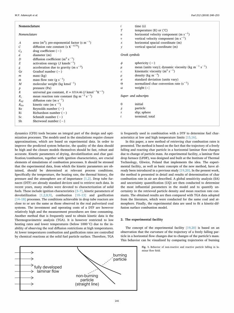
The concept of the experimental facility [19,20] is based on anobservation that the curvature of the trajectory of a freely falling par-ticle in a horizontal flow changes due to changes of the particle’s mass.This behavior can be visualized by comparing trajectories of burning

Nomenclature

Nomenclature

A area (m2); pre-exponential factor (s m−1)C diffusion rate constant (s K−0.75)Cd drag coefficient (−)d diameter (m)D diffusion coefficient (m2 s−1)E activation energy (J kmols−1)g acceleration due to gravity (m s−2)Gr Grashof number (−)m mass (kg)m mass flow rate (g s−1)M molecular weight (kg kmol−1)p pressure (Pa)R universal gas constant, =R 8314.46 (J kmol−1K−1)Rc mean reaction rate constant (kg m−2 s−1)Rdif diffusion rate (m s−1)Rkin kinetic rate (m s−1)Re Reynolds number (−)Ri Richardson number (−)Sc Schmidt number (−)Sh Sherwood number (−)

t time (s)T temperature (K) or (°C)u horizontal velocity component (m s−1)v vertical velocity component (m s−1)x horizontal spacial coordinate (m)y vertical spacial coordinate (m)

Greek symbols

ϕ sphericity (−)μ mean (units vary); dynamic viscosity (kg m−1 s−1)ν kinematic viscosity (m2 s−1)ρ density (kg m−3)σ standard deviation (units vary)Θ normalized char conversion rate (s−1)ω weight −( )

Super- and subscripts

0 initialp particles slip; spheret terminal; total

Fig. 1. Behavior of non-reactive and reactive particle falling in la-minar flow field.

W.P. Adamczyk et al. Fuel 212 (2018) 240–255

241

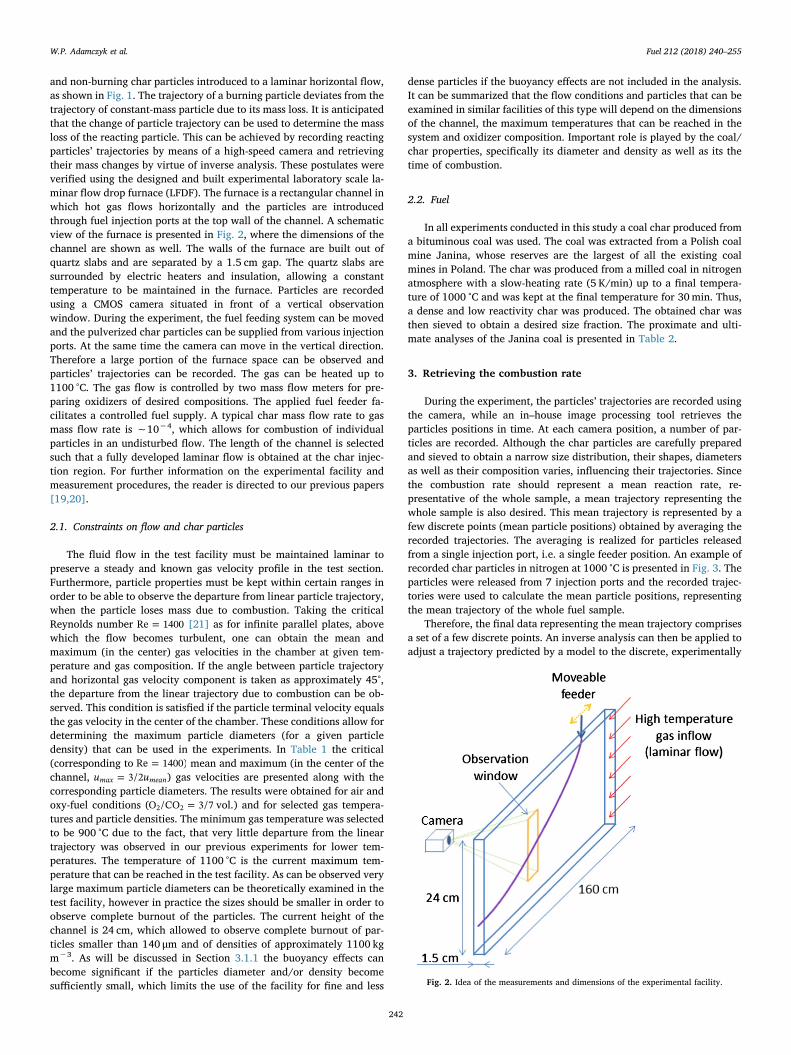
and non-burning char particles introduced to a laminar horizontal flow,as shown in Fig. 1. The trajectory of a burning particle deviates from thetrajectory of constant-mass particle due to its mass loss. It is anticipatedthat the change of particle trajectory can be used to determine the massloss of the reacting particle. This can be achieved by recording reactingparticles’ trajectories by means of a high-speed camera and retrievingtheir mass changes by virtue of inverse analysis. These postulates wereverified using the designed and built experimental laboratory scale la-minar flow drop furnace (LFDF). The furnace is a rectangular channel inwhich hot gas flows horizontally and the particles are introducedthrough fuel injection ports at the top wall of the channel. A schematicview of the furnace is presented in Fig. 2, where the dimensions of thechannel are shown as well. The walls of the furnace are built out ofquartz slabs and are separated by a 1.5 cm gap. The quartz slabs aresurrounded by electric heaters and insulation, allowing a constanttemperature to be maintained in the furnace. Particles are recordedusing a CMOS camera situated in front of a vertical observationwindow. During the experiment, the fuel feeding system can be movedand the pulverized char particles can be supplied from various injectionports. At the same time the camera can move in the vertical direction.Therefore a large portion of the furnace space can be observed andparticles’ trajectories can be recorded. The gas can be heated up to1100 °C. The gas flow is controlled by two mass flow meters for pre-paring oxidizers of desired compositions. The applied fuel feeder fa-cilitates a controlled fuel supply. A typical char mass flow rate to gasmass flow rate is ∼10−4, which allows for combustion of individualparticles in an undisturbed flow. The length of the channel is selectedsuch that a fully developed laminar flow is obtained at the char injec-tion region. For further information on the experimental facility andmeasurement procedures, the reader is directed to our previous papers[19,20].

2.1. Constraints on flow and char particles

The fluid flow in the test facility must be maintained laminar topreserve a steady and known gas velocity profile in the test section.Furthermore, particle properties must be kept within certain ranges inorder to be able to observe the departure from linear particle trajectory,when the particle loses mass due to combustion. Taking the criticalReynolds number =Re 1400 [21] as for infinite parallel plates, abovewhich the flow becomes turbulent, one can obtain the mean andmaximum (in the center) gas velocities in the chamber at given tem-perature and gas composition. If the angle between particle trajectoryand horizontal gas velocity component is taken as approximately 45°,the departure from the linear trajectory due to combustion can be ob-served. This condition is satisfied if the particle terminal velocity equalsthe gas velocity in the center of the chamber. These conditions allow fordetermining the maximum particle diameters (for a given particledensity) that can be used in the experiments. In Table 1 the critical(corresponding to =Re 1400) mean and maximum (in the center of thechannel, =u u3/2max mean) gas velocities are presented along with thecorresponding particle diameters. The results were obtained for air andoxy-fuel conditions ( =O /CO 3/72 2 vol.) and for selected gas tempera-tures and particle densities. The minimum gas temperature was selectedto be 900 °C due to the fact, that very little departure from the lineartrajectory was observed in our previous experiments for lower tem-peratures. The temperature of 1100 °C is the current maximum tem-perature that can be reached in the test facility. As can be observed verylarge maximum particle diameters can be theoretically examined in thetest facility, however in practice the sizes should be smaller in order toobserve complete burnout of the particles. The current height of thechannel is 24 cm, which allowed to observe complete burnout of par-ticles smaller than 140 μm and of densities of approximately 1100 kgm−3. As will be discussed in Section 3.1.1 the buoyancy effects canbecome significant if the particles diameter and/or density becomesufficiently small, which limits the use of the facility for fine and less

dense particles if the buoyancy effects are not included in the analysis.It can be summarized that the flow conditions and particles that can beexamined in similar facilities of this type will depend on the dimensionsof the channel, the maximum temperatures that can be reached in thesystem and oxidizer composition. Important role is played by the coal/char properties, specifically its diameter and density as well as its thetime of combustion.

2.2. Fuel

In all experiments conducted in this study a coal char produced froma bituminous coal was used. The coal was extracted from a Polish coalmine Janina, whose reserves are the largest of all the existing coalmines in Poland. The char was produced from a milled coal in nitrogenatmosphere with a slow-heating rate (5 K/min) up to a final tempera-ture of 1000 °C and was kept at the final temperature for 30min. Thus,a dense and low reactivity char was produced. The obtained char wasthen sieved to obtain a desired size fraction. The proximate and ulti-mate analyses of the Janina coal is presented in Table 2.

3. Retrieving the combustion rate

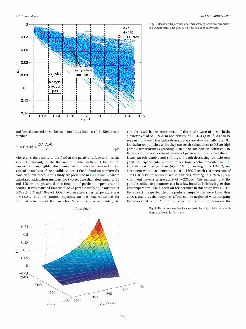
During the experiment, the particles’ trajectories are recorded usingthe camera, while an in–house image processing tool retrieves theparticles positions in time. At each camera position, a number of par-ticles are recorded. Although the char particles are carefully preparedand sieved to obtain a narrow size distribution, their shapes, diametersas well as their composition varies, influencing their trajectories. Sincethe combustion rate should represent a mean reaction rate, re-presentative of the whole sample, a mean trajectory representing thewhole sample is also desired. This mean trajectory is represented by afew discrete points (mean particle positions) obtained by averaging therecorded trajectories. The averaging is realized for particles releasedfrom a single injection port, i.e. a single feeder position. An example ofrecorded char particles in nitrogen at 1000 °C is presented in Fig. 3. Theparticles were released from 7 injection ports and the recorded trajec-tories were used to calculate the mean particle positions, representingthe mean trajectory of the whole fuel sample.

Therefore, the final data representing the mean trajectory comprisesa set of a few discrete points. An inverse analysis can then be applied toadjust a trajectory predicted by a model to the discrete, experimentally

Fig. 2. Idea of the measurements and dimensions of the experimental facility.

W.P. Adamczyk et al. Fuel 212 (2018) 240–255

242

determined particle positions. For this, a model, which allows for cal-culating a reactive particle trajectory, has to be formulated. The modelcomprises the direct problem in the inverse analysis.

3.1. The direct problem

The model equations are formulated based on the forces acting on asingle particle. In this study, the acceleration of the particle is attributedsolely to the balance between the gravitational force and the drag. Theforce balance together with the definitions of the particle velocitiesform the equations from which x t( )p and y t( )p can be calculated. Theseare the equations for particle velocity in x direction

=xt

udd

pp (1)

particle velocity in y direction

=yt

vdd

pp (2)

particle acceleration in x direction

= −ut

μρ d

C u udd

18 Re24

( )p

p pd

pp2

(3)

particle acceleration in y direction

= − +−v

tμ

ρ dC v v

g ρ ρρ

dd

18 Re24

( )( )p

p pd

pp

p

p2

(4)

where up and vp are the particle velocities in the x and y direction,respectively, ρp and dp are particle density and diameter, ρ and μ are thedensity and dynamic viscosity of the fluid, Cd is the drag coefficient, uand v are gas velocities in x and y direction, g is the gravitational ac-celeration and Rep is the particle Reynolds number defined as

=ρd u

μRep

p s

(5)

where us is the relative velocity of the fluid with respect to particlevelocity; such that = −u u u| |s p in the x direction and = −u v v| |s p in the ydirection. The drag coefficient is determined using the correlations byHaider and Levenspiel [22], which take into account the sphericity ϕ ofthe particles. The sphericity is defined as

=ϕ AA

s

p (6)

where As is the surface area of a sphere having the same volume as the

particle and Ap is the actual surface area of the particle.At the current stage of development of the methodology, it is as-

sumed that a mean particle conversion rate is to be determined. Therate of change of mass is assumed to be

= −mt

R πddd

pc p

2(7)

where mp is the particle mass and Rc is the mean reaction rate constantin kg m−2s−1. The mean reaction rate constant Rc encompasses all thecomplex physico-chemical processes that occur during particle con-version and thus is a drastic simplification of the reality, however forthe current stage of development, it is desirable to limit the number ofunknowns and to represent the conversion process by a global para-meter. Such an approach allows for analysis of the parameters influ-encing the determination of the reaction rate.

Eq. (7) is coupled with the set of Eq. (1)–(4) by the particle density

=ρm

πd6

pp

p3

(8)

If Rc is known, solving the above set of equations allows de-termining the particle trajectory (x t( )p and y t( )p ) for a reacting particle.The solution is subject to the following initial conditions

⎧

⎨

⎪⎪

⎩

⎪⎪

==== −=

xyuv vm ρ πd

(0) 0(0) 0(0) 0(0)

(0) /6

p

p

p

p t

p p p0 03

(9)

where ρp0 and dp0 are the initial particle density and diameter, respec-tively and vt is the terminal velocity, i.e., the maximum free fall velocityof the particle determined at the conditions of the flow. Justification forthe terminal velocity used as the boundary condition will be presentedin Section 3.1.5. It is assumed that the flow of particles is two dimen-sional x y( , ), therefore the possible deviation of the particle’s trajectoryin the z direction is ignored. This is justified due to a narrow depth offield (∼3mm) of the camera that was used in the experiments. Ananalysis of the velocity profile variation in the channel leads to a con-clusion that the particles falling within the 3mm depth of field can beexposed to gas velocity differing at most by 4%. The algorithm used todetermine the particle positions from recorded images accepts onlysharp particle images, so that the particles that are not in the center ofthe reactor are ignored. From the experience gained so far, only a smallpercentage of the particles fall outside the depth of field. This allowsone to assume that the observed particles flow in the gas of maximumvelocity u, which is in the center of the reactor.

3.1.1. Buoyancy effectsFurther assumption of this study is that the gas density ρ entering

Eqs. (4) and (5) is constant for a given test and equal to the density ofthe free stream air. The reason of this assumption is the lack of possi-bility measuring the burning particle temperature. Therefore thebuoyancy effects associated with the increase of gas temperature nearthe particle surface and the net outflow of CO and CO2 from the particlesurface are neglected at the current stage of development of themethodology. As discussed by Richter et al. [23], this assumption isjustified at certain conditions only. The importance of the buoyancy

Table 1Limiting conditions of the facility.

air O2/CO2= 3/7

T (°C) 900 1100 900 1100umean (m s−1) 14.8 19.2 10.6 13.8umax (m s−1) 22.2 28.8 15.9 20.7

ρp (kgm−3) dp (mm)

600 8.7 11.8 6.7 9.0900 6.2 8.4 4.9 6.51200 5.0 6.7 3.9 5.2

Table 2Proximate and ultimate analyses of the Janina coal.

Proximate analysis (wt.% ar) Ultimate analysis (wt.% db) Higher heating value (M J kg−1 ar)

Moist. Ash Vol. c h o n s HHV11.0 12.28 30.43 65.44 4.48 13.55 1.02 1.71 22.910

ar – as received; db – dry basis.

W.P. Adamczyk et al. Fuel 212 (2018) 240–255

243

and forced convection can be examined by estimation of the Richardsonnumber

= =−g ρ ρ dρ ν

Ri Gr/Re( )

ps p

s

23

2 (10)

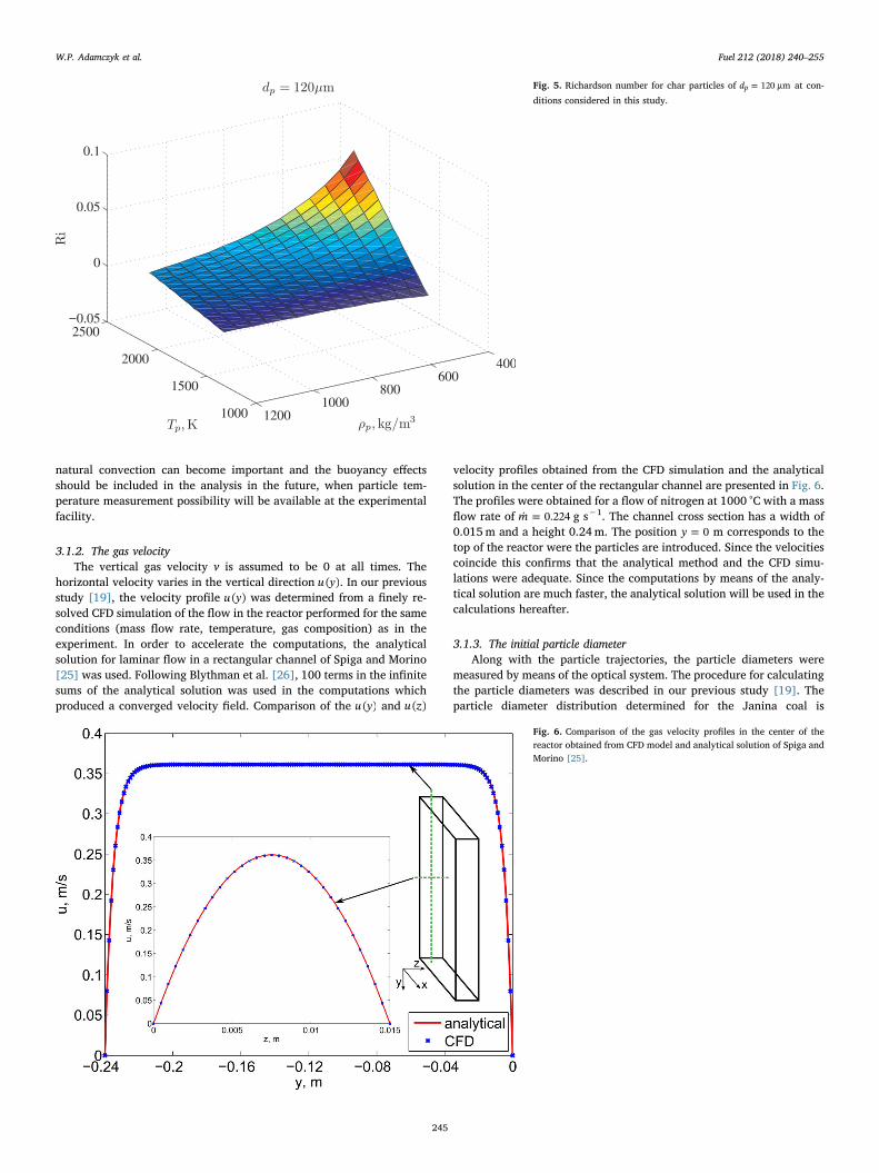
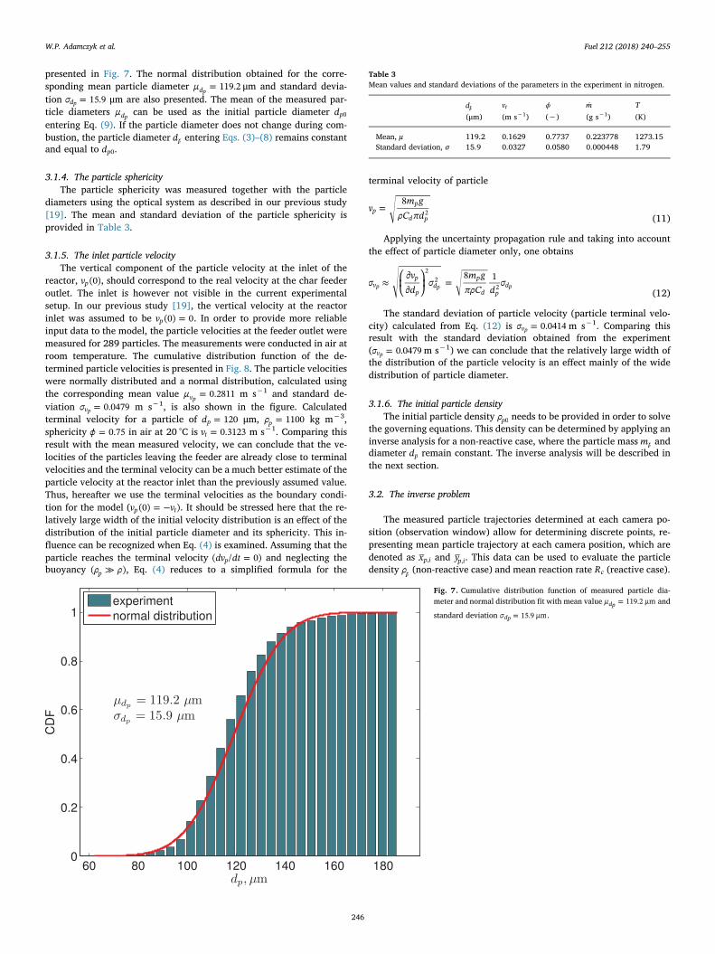
where ρs is the density of the fluid at the particle surface and ν is thekinematic viscosity. If the Richardson number is <Ri 0.1 the naturalconvection is negligible when compared to the forced convection. Re-sults of an analysis of the possible values of the Richardson numbers forconditions examined in this study are presented in Figs. 4 and 5, wherecalculated Richardson numbers for two particle diameters equal to 80and 120 μm are presented as a function of particle temperature anddensity. It was assumed that the fluid at particle surface is a mixture of50% vol. CO and 50% vol. CO2, the free stream gas temperature was

=T 1323 K and the particle Reynolds number was calculated forterminal velocities of the particles. As will be discussed later, the

particles used in the experiments of this study were of mean initialdiameter equal to 119.2 μm and density of 1076.4 kg m−3. As can beseen in Fig. 4 and 5 the Richardson numbers are always smaller than 0.1for the larger particles, while they can reach values close to 0.3 for highparticle temperatures exceeding 2000 K and low particle densities. Thelatter conditions can occur at the end of particle burnout, where there islower particle density and still high, though decreasing, particle tem-perature. Experiments in an entrained flow reactor presented in [24]indicate that char particles ( ∼dp 115μm) burning in a 12% O2 en-vironment with a gas temperature of ∼1600 K reach a temperature of∼2000 K prior to burnout, while particles burning in a 24% O2 en-vironment have a temperature of ∼2200 K. This indicates that theparticle surface temperatures can be a few hundred Kelvins higher thangas temperature. The highest air temperature in this study was 1323 K,therefore it is expected that the particle temperatures were lower than2000 K and thus the buoyancy effects can be neglected with acceptingthe associated error. At the last stages of combustion, however the

Fig. 3. Recorded trajectories and their average positions comprisingthe experimental data used to retrieve the char conversion.

Fig. 4. Richardson number for char particles of =d 80 μmp at condi-

tions considered in this study.

W.P. Adamczyk et al. Fuel 212 (2018) 240–255

244

natural convection can become important and the buoyancy effectsshould be included in the analysis in the future, when particle tem-perature measurement possibility will be available at the experimentalfacility.

3.1.2. The gas velocityThe vertical gas velocity v is assumed to be 0 at all times. The

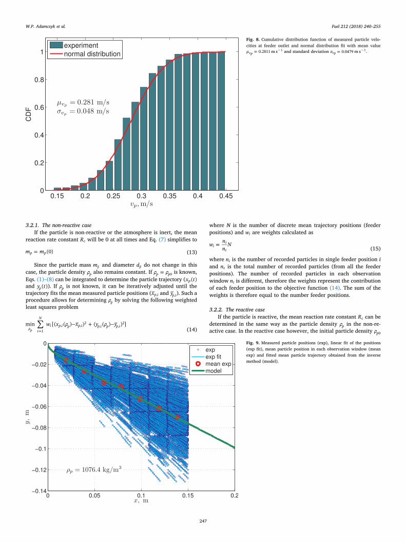
horizontal velocity varies in the vertical direction u y( ). In our previousstudy [19], the velocity profile u y( ) was determined from a finely re-solved CFD simulation of the flow in the reactor performed for the sameconditions (mass flow rate, temperature, gas composition) as in theexperiment. In order to accelerate the computations, the analyticalsolution for laminar flow in a rectangular channel of Spiga and Morino[25] was used. Following Blythman et al. [26], 100 terms in the infinitesums of the analytical solution was used in the computations whichproduced a converged velocity field. Comparison of the u y( ) and u z( )

velocity profiles obtained from the CFD simulation and the analyticalsolution in the center of the rectangular channel are presented in Fig. 6.The profiles were obtained for a flow of nitrogen at 1000 °C with a massflow rate of =m 0.224 g s−1. The channel cross section has a width of0.015m and a height 0.24m. The position =y 0 m corresponds to thetop of the reactor were the particles are introduced. Since the velocitiescoincide this confirms that the analytical method and the CFD simu-lations were adequate. Since the computations by means of the analy-tical solution are much faster, the analytical solution will be used in thecalculations hereafter.

3.1.3. The initial particle diameterAlong with the particle trajectories, the particle diameters were

measured by means of the optical system. The procedure for calculatingthe particle diameters was described in our previous study [19]. Theparticle diameter distribution determined for the Janina coal is

Fig. 5. Richardson number for char particles of =d 120 μmp at con-

ditions considered in this study.

Fig. 6. Comparison of the gas velocity profiles in the center of thereactor obtained from CFD model and analytical solution of Spiga andMorino [25].

W.P. Adamczyk et al. Fuel 212 (2018) 240–255

245

presented in Fig. 7. The normal distribution obtained for the corre-sponding mean particle diameter =μ 119.2dp μm and standard devia-tion =σ 15.9dp μm are also presented. The mean of the measured par-ticle diameters μdp can be used as the initial particle diameter dp0

entering Eq. (9). If the particle diameter does not change during com-bustion, the particle diameter dp entering Eqs. (3)–(8) remains constantand equal to dp0.

3.1.4. The particle sphericityThe particle sphericity was measured together with the particle

diameters using the optical system as described in our previous study[19]. The mean and standard deviation of the particle sphericity isprovided in Table 3.

3.1.5. The inlet particle velocityThe vertical component of the particle velocity at the inlet of the

reactor, v (0)p , should correspond to the real velocity at the char feederoutlet. The inlet is however not visible in the current experimentalsetup. In our previous study [19], the vertical velocity at the reactorinlet was assumed to be =v (0) 0p . In order to provide more reliableinput data to the model, the particle velocities at the feeder outlet weremeasured for 289 particles. The measurements were conducted in air atroom temperature. The cumulative distribution function of the de-termined particle velocities is presented in Fig. 8. The particle velocitieswere normally distributed and a normal distribution, calculated usingthe corresponding mean value =μ 0.2811vp m s−1 and standard de-viation =σ 0.0479vp m s−1, is also shown in the figure. Calculatedterminal velocity for a particle of =d 120p μm, =ρ 1100p kg m−3,sphericity =ϕ 0.75 in air at 20 °C is =v 0.3123t m s−1. Comparing thisresult with the mean measured velocity, we can conclude that the ve-locities of the particles leaving the feeder are already close to terminalvelocities and the terminal velocity can be a much better estimate of theparticle velocity at the reactor inlet than the previously assumed value.Thus, hereafter we use the terminal velocities as the boundary condi-tion for the model ( = −v v(0) )p t . It should be stressed here that the re-latively large width of the initial velocity distribution is an effect of thedistribution of the initial particle diameter and its sphericity. This in-fluence can be recognized when Eq. (4) is examined. Assuming that theparticle reaches the terminal velocity =dv dt( / 0)p and neglecting thebuoyancy ≫ρ ρ( )p , Eq. (4) reduces to a simplified formula for the

terminal velocity of particle

=vm g

ρC πd8

pp

d p2

(11)

Applying the uncertainty propagation rule and taking into accountthe effect of particle diameter only, one obtains

⎜ ⎟≈ ⎛⎝

∂∂

⎞⎠

=σvd

σm g

πρC dσ

8 1v

p

pd

p

d pd

22

2p p p(12)

The standard deviation of particle velocity (particle terminal velo-city) calculated from Eq. (12) is =σ 0.0414vp m s−1. Comparing thisresult with the standard deviation obtained from the experiment( =σ 0.0479vp m s−1) we can conclude that the relatively large width ofthe distribution of the particle velocity is an effect mainly of the widedistribution of particle diameter.

3.1.6. The initial particle densityThe initial particle density ρp0 needs to be provided in order to solve

the governing equations. This density can be determined by applying aninverse analysis for a non-reactive case, where the particle mass mp anddiameter dp remain constant. The inverse analysis will be described inthe next section.

3.2. The inverse problem

The measured particle trajectories determined at each camera po-sition (observation window) allow for determining discrete points, re-presenting mean particle trajectory at each camera position, which aredenoted as xp i, and yp i, . This data can be used to evaluate the particledensity ρp (non-reactive case) and mean reaction rate Rc (reactive case).

Fig. 7. Cumulative distribution function of measured particle dia-meter and normal distribution fit with mean value =μ 119.2 μmdp and

standard deviation =σ 15.9 μmdp .

Table 3Mean values and standard deviations of the parameters in the experiment in nitrogen.

dp vt ϕ m T

(μm) (m s−1) (−) (g s−1) (K)

Mean, μ 119.2 0.1629 0.7737 0.223778 1273.15Standard deviation, σ 15.9 0.0327 0.0580 0.000448 1.79

W.P. Adamczyk et al. Fuel 212 (2018) 240–255

246

3.2.1. The non-reactive caseIf the particle is non-reactive or the atmosphere is inert, the mean

reaction rate constant Rc will be 0 at all times and Eq. (7) simplifies to

=m m (0)p p (13)

Since the particle mass mp and diameter dp do not change in thiscase, the particle density ρp also remains constant. If =ρ ρp p0 is known,Eqs. (1)–(8) can be integrated to determine the particle trajectory (x t( )pand y t( )p ). If ρp is not known, it can be iteratively adjusted until thetrajectory fits the mean measured particle positions (xp i, and yp i, ). Such aprocedure allows for determining ρp by solving the following weightedleast squares problem

∑ − + −=

w x ρ x y ρ ymin [( ( ) ) ( ( ) ) ]ρ i

N

i p i p p i p i p p i1

, ,2

, ,2

p (14)

where N is the number of discrete mean trajectory positions (feederpositions) and wi are weights calculated as

=w nn

Nii

t (15)

where ni is the number of recorded particles in single feeder position iand nt is the total number of recorded particles (from all the feederpositions). The number of recorded particles in each observationwindow ni is different, therefore the weights represent the contributionof each feeder position to the objective function (14). The sum of theweights is therefore equal to the number feeder positions.

3.2.2. The reactive caseIf the particle is reactive, the mean reaction rate constant Rc can be

determined in the same way as the particle density ρp in the non-re-active case. In the reactive case however, the initial particle density ρp0

Fig. 8. Cumulative distribution function of measured particle velo-cities at feeder outlet and normal distribution fit with mean value

=μ 0.2811vp m s−1 and standard deviation =σ 0.0479vp m s−1.

Fig. 9. Measured particle positions (exp), linear fit of the positions(exp fit), mean particle position in each observation window (meanexp) and fitted mean particle trajectory obtained from the inversemethod (model).

W.P. Adamczyk et al. Fuel 212 (2018) 240–255

247

must be known and it is determined from the non-reactive case. In orderto find the mean reaction rate Rc, the following minimization problemis then solved

∑ − + −=

w x R x y R ymin [( ( ) ) ( ( ) ) ]R i

N

i p i c p i p i c p i1

, ,2

, ,2

c (16)

3.2.3. Numerical solutionThe sets of ordinary differential equations for non-reactive and re-

active cases are solved using the explicit Runge–Kutta (4,5) method andthe minimization problem is solved using the Pattern Search solver,both implemented in MATLAB [27].

4. Results and discussion

4.1. The non-reactive case

As mentioned earlier the material density of the particles can bedetermined by conducting non-reactive experiments. The non-reactiveexperiment was conducted for the Janina coal char. The char wasmilled and sieved to obtain a narrow particle size distribution. Theexperiment was conducted in nitrogen at 1000 °C. The mass flow rate ofthe carrier nitrogen was 0.224 gs−1. The resulting measured particlepositions are presented in Fig. 9. The positions were then approximatedby a linear function (exp fit) and a mean particle position was computedin each observation window (mean exp). As can be observed, the non-reacting particles follow straight lines and the particles form an ex-panding cloud of trajectories. The reason for the large spread of theparticles positions are the natural in–homogeneous properties of in-dividual particles, which include diameter, shape, ash content, etc.Although the particles were sieved before the experiment with a sievemesh size difference of 5 μm the size distribution is much wider (cf.Fig. 7) due to the longitudinal shape of some fraction of the particlesand inaccuracy of the optical measurement. All these factors influencethe broadening of the cloud.

The mean positions (mean exp) presented in Fig. 9 were then usedin the inverse analysis to find the particle density ρp. The data requiredto perform the inverse analysis are presented in Table 3. The tablecontains also the standard deviations of the data, which will be used inthe forthcoming section for sensitivity analysis and uncertainty quan-tification. The standard deviations were not required for the current

calculations. The particle material density obtained from the inverseanalysis is =ρ 1076.4p kg m−3. The corresponding mean particle tra-jectory (model) is presented in Fig. 9 as well. Initially, the modeledparticle falls into the chamber with initial vertical velocity component

= −v v(0)p t and passes the boundary layer (cf. Fig. 6) virtually withoutany horizontal displacement. As it becomes exposed to higher gas ve-locities, its horizontal velocity component vp becomes larger up to apoint where the forces acting on the particle equilibrate and the particlestarts to follow a straight line. This is due to the fact that the particlemass does not change, and the gas velocity is virtually constant, outsidethe boundary layer. As can be seen, the fitted trajectory follows theexperimentally determined mean particle positions and thus, it is re-presentative for all the particles. The determined particle materialdensity was then used as the initial density in the reactive experiments.

4.2. The reactive cases

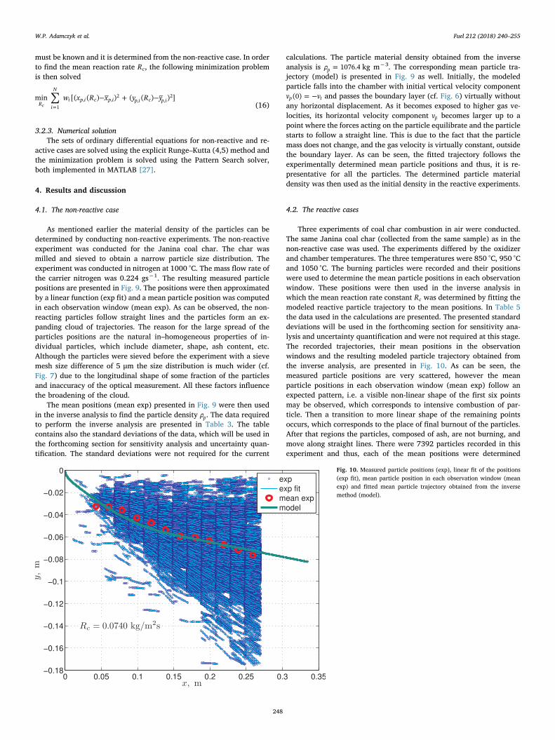
Three experiments of coal char combustion in air were conducted.The same Janina coal char (collected from the same sample) as in thenon-reactive case was used. The experiments differed by the oxidizerand chamber temperatures. The three temperatures were 850 °C, 950 °Cand 1050 °C. The burning particles were recorded and their positionswere used to determine the mean particle positions in each observationwindow. These positions were then used in the inverse analysis inwhich the mean reaction rate constant Rc was determined by fitting themodeled reactive particle trajectory to the mean positions. In Table 5the data used in the calculations are presented. The presented standarddeviations will be used in the forthcoming section for sensitivity ana-lysis and uncertainty quantification and were not required at this stage.The recorded trajectories, their mean positions in the observationwindows and the resulting modeled particle trajectory obtained fromthe inverse analysis, are presented in Fig. 10. As can be seen, themeasured particle positions are very scattered, however the meanparticle positions in each observation window (mean exp) follow anexpected pattern, i.e. a visible non-linear shape of the first six pointsmay be observed, which corresponds to intensive combustion of par-ticle. Then a transition to more linear shape of the remaining pointsoccurs, which corresponds to the place of final burnout of the particles.After that regions the particles, composed of ash, are not burning, andmove along straight lines. There were 7392 particles recorded in thisexperiment and thus, each of the mean positions were determined

Fig. 10. Measured particle positions (exp), linear fit of the positions(exp fit), mean particle position in each observation window (meanexp) and fitted mean particle trajectory obtained from the inversemethod (model).

W.P. Adamczyk et al. Fuel 212 (2018) 240–255

248

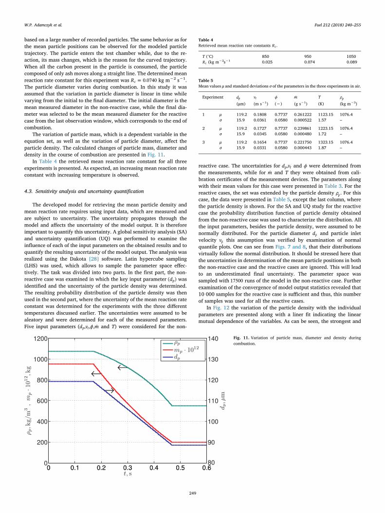
based on a large number of recorded particles. The same behavior as forthe mean particle positions can be observed for the modeled particletrajectory. The particle enters the test chamber while, due to the re-action, its mass changes, which is the reason for the curved trajectory.When all the carbon present in the particle is consumed, the particlecomposed of only ash moves along a straight line. The determined meanreaction rate constant for this experiment was =R 0.0740c kg m−2 s−1.The particle diameter varies during combustion. In this study it wasassumed that the variation in particle diameter is linear in time whilevarying from the initial to the final diameter. The initial diameter is themean measured diameter in the non-reactive case, while the final dia-meter was selected to be the mean measured diameter for the reactivecase from the last observation window, which corresponds to the end ofcombustion.

The variation of particle mass, which is a dependent variable in theequation set, as well as the variation of particle diameter, affect theparticle density. The calculated changes of particle mass, diameter anddensity in the course of combustion are presented in Fig. 11.

In Table 4 the retrieved mean reaction rate constant for all threeexperiments is presented. As expected, an increasing mean reaction rateconstant with increasing temperature is observed.

4.3. Sensitivity analysis and uncertainty quantification

The developed model for retrieving the mean particle density andmean reaction rate requires using input data, which are measured andare subject to uncertainty. The uncertainty propagates through themodel and affects the uncertainty of the model output. It is thereforeimportant to quantify this uncertainty. A global sensitivity analysis (SA)and uncertainty quantification (UQ) was performed to examine theinfluence of each of the input parameters on the obtained results and toquantify the resulting uncertainty of the model output. The analysis wasrealized using the Dakota [28] software. Latin hypercube sampling(LHS) was used, which allows to sample the parameter space effec-tively. The task was divided into two parts. In the first part, the non-reactive case was examined in which the key input parameter d( )p wasidentified and the uncertainty of the particle density was determined.The resulting probability distribution of the particle density was thenused in the second part, where the uncertainty of the mean reaction rateconstant was determined for the experiments with the three differenttemperatures discussed earlier. The uncertainties were assumed to bealeatory and were determined for each of the measured parameters.Five input parameters (d v ϕ m, , , p t and T) were considered for the non-

reactive case. The uncertainties for d v,p t and ϕ were determined fromthe measurements, while for m and T they were obtained from cali-bration certificates of the measurement devices. The parameters alongwith their mean values for this case were presented in Table 3. For thereactive cases, the set was extended by the particle density ρp. For thiscase, the data were presented in Table 5, except the last column, wherethe particle density is shown. For the SA and UQ study for the reactivecase the probability distribution function of particle density obtainedfrom the non-reactive case was used to characterize the distribution. Allthe input parameters, besides the particle density, were assumed to benormally distributed. For the particle diameter dp and particle inletvelocity vp this assumption was verified by examination of normalquantile plots. One can see from Figs. 7 and 8, that their distributionsvirtually follow the normal distribution. It should be stressed here thatthe uncertainties in determination of the mean particle positions in boththe non-reactive case and the reactive cases are ignored. This will leadto an underestimated final uncertainty. The parameter space wassampled with 17500 runs of the model in the non-reactive case. Furtherexamination of the convergence of model output statistics revealed that10 000 samples for the reactive case is sufficient and thus, this numberof samples was used for all the reactive cases.

In Fig. 12 the variation of the particle density with the individualparameters are presented along with a liner fit indicating the linearmutual dependence of the variables. As can be seen, the strongest and

Fig. 11. Variation of particle mass, diameter and density duringcombustion.

Table 4Retrieved mean reaction rate constants Rc .

T (°C) 850 950 1050Rc (kg m−2s−1 0.025 0.074 0.089

Table 5Mean values μ and standard deviations σ of the parameters in the three experiments in air.

Experiment dp vt ϕ m T ρp

(μm) (m s−1) (−) (g s−1) (K) (kg m−3)

1 μ 119.2 0.1808 0.7737 0.261222 1123.15 1076.4σ 15.9 0.0361 0.0580 0.000522 1.57 –

2 μ 119.2 0.1727 0.7737 0.239861 1223.15 1076.4σ 15.9 0.0345 0.0580 0.000480 1.72 –

3 μ 119.2 0.1654 0.7737 0.221750 1323.15 1076.4σ 15.9 0.0331 0.0580 0.000443 1.87 –

W.P. Adamczyk et al. Fuel 212 (2018) 240–255

249

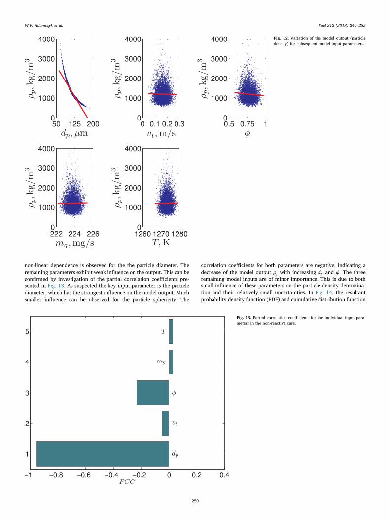
non-linear dependence is observed for the the particle diameter. Theremaining parameters exhibit weak influence on the output. This can beconfirmed by investigation of the partial correlation coefficients pre-sented in Fig. 13. As suspected the key input parameter is the particlediameter, which has the strongest influence on the model output. Muchsmaller influence can be observed for the particle sphericity. The

correlation coefficients for both parameters are negative, indicating adecrease of the model output ρp with increasing dp and ϕ. The threeremaining model inputs are of minor importance. This is due to bothsmall influence of these parameters on the particle density determina-tion and their relatively small uncertainties. In Fig. 14, the resultantprobability density function (PDF) and cumulative distribution function

Fig. 12. Variation of the model output (particledensity) for subsequent model input parameters.

Fig. 13. Partial correlation coefficients for the individual input para-meters in the non-reactive case.

W.P. Adamczyk et al. Fuel 212 (2018) 240–255

250

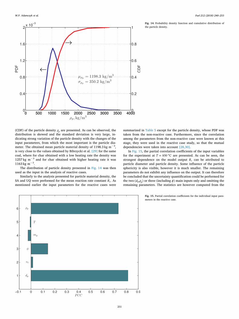
(CDF) of the particle density ρp are presented. As can be observed, thedistribution is skewed and the standard deviation is very large, in-dicating strong variation of the particle density with the changes of theinput parameters, from which the most important is the particle dia-meter. The obtained mean particle material density of 1198.3 kg m−3,is very close to the values obtained by Bibrzycki et al. [29] for the samecoal, where for char obtained with a low heating rate the density was1257 kg m−3 and for char obtained with higher heating rate it was1163 kg m−3.

The distribution of particle density presented in Fig. 14 was thenused as the input in the analysis of reactive cases.

Similarly to the analysis presented for particle material density, theSA and UQ were performed for the mean reaction rate constant Rc. Asmentioned earlier the input parameters for the reactive cases were

summarized in Table 5 except for the particle density, whose PDF wastaken from the non-reactive case. Furthermore, since the correlationamong the parameters from the non-reactive case were known at thisstage, they were used in the reactive case study, so that the mutualdependencies were taken into account [28,30].

In Fig. 15, the partial correlation coefficients of the input variablesfor the experiment at = °T 850 C are presented. As can be seen, thestrongest dependence on the model output Rc can be attributed toparticle diameter and particle density. Some influence of the particlesphericity is also visible, however it is much smaller. The remainingparameters do not exhibit any influence on the output. It can thereforebe concluded that the uncertainty quantification could be performed forthe two d ρ( , )p p or three (including ϕ) main inputs only and omitting theremaining parameters. The statistics are however computed from the

Fig. 14. Probability density function and cumulative distribution ofthe particle density.

Fig. 15. Partial correlation coefficients for the individual input para-meters in the reactive case.

W.P. Adamczyk et al. Fuel 212 (2018) 240–255

251

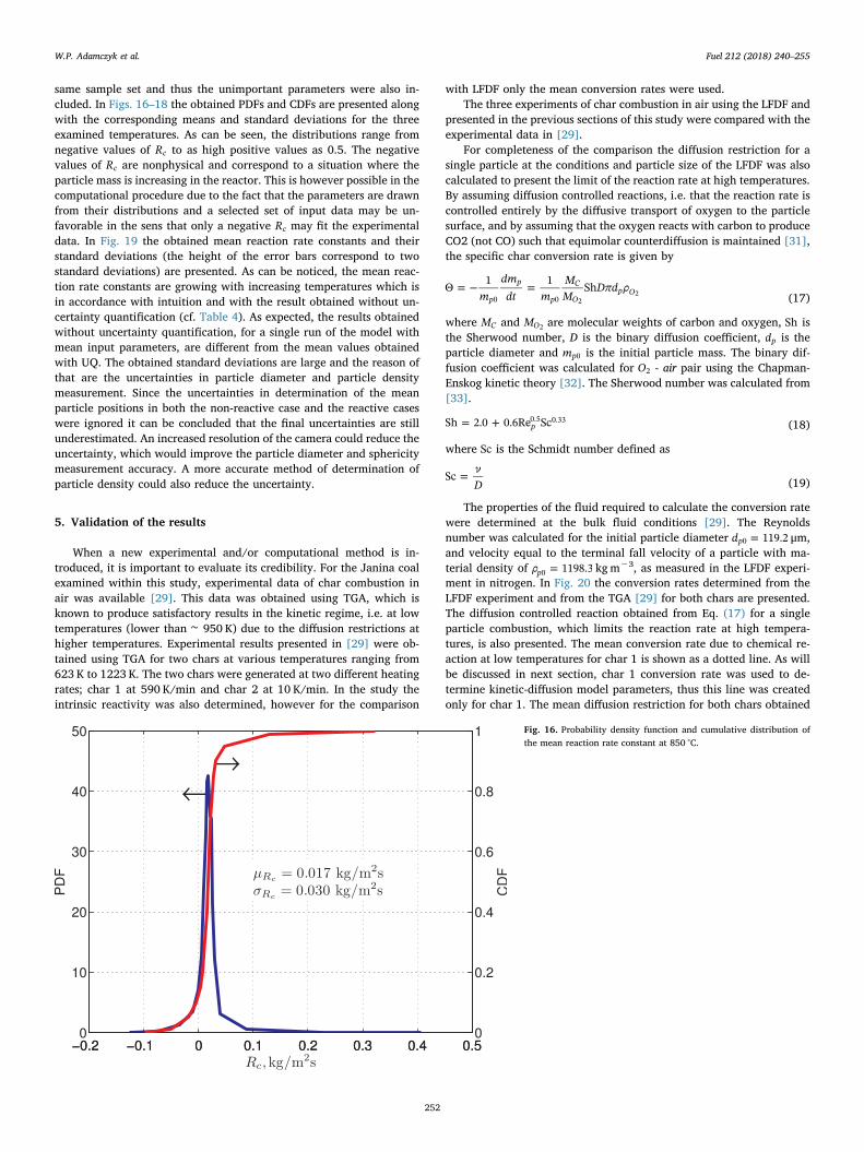
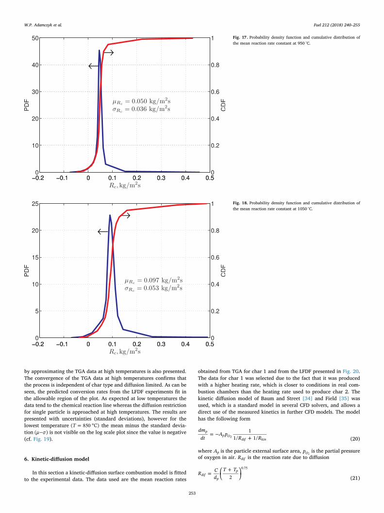
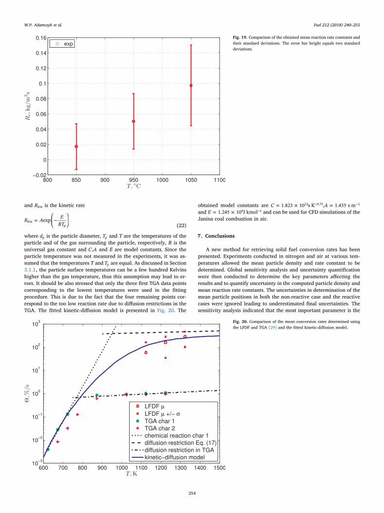
same sample set and thus the unimportant parameters were also in-cluded. In Figs. 16–18 the obtained PDFs and CDFs are presented alongwith the corresponding means and standard deviations for the threeexamined temperatures. As can be seen, the distributions range fromnegative values of Rc to as high positive values as 0.5. The negativevalues of Rc are nonphysical and correspond to a situation where theparticle mass is increasing in the reactor. This is however possible in thecomputational procedure due to the fact that the parameters are drawnfrom their distributions and a selected set of input data may be un-favorable in the sens that only a negative Rc may fit the experimentaldata. In Fig. 19 the obtained mean reaction rate constants and theirstandard deviations (the height of the error bars correspond to twostandard deviations) are presented. As can be noticed, the mean reac-tion rate constants are growing with increasing temperatures which isin accordance with intuition and with the result obtained without un-certainty quantification (cf. Table 4). As expected, the results obtainedwithout uncertainty quantification, for a single run of the model withmean input parameters, are different from the mean values obtainedwith UQ. The obtained standard deviations are large and the reason ofthat are the uncertainties in particle diameter and particle densitymeasurement. Since the uncertainties in determination of the meanparticle positions in both the non-reactive case and the reactive caseswere ignored it can be concluded that the final uncertainties are stillunderestimated. An increased resolution of the camera could reduce theuncertainty, which would improve the particle diameter and sphericitymeasurement accuracy. A more accurate method of determination ofparticle density could also reduce the uncertainty.

5. Validation of the results

When a new experimental and/or computational method is in-troduced, it is important to evaluate its credibility. For the Janina coalexamined within this study, experimental data of char combustion inair was available [29]. This data was obtained using TGA, which isknown to produce satisfactory results in the kinetic regime, i.e. at lowtemperatures (lower than ∼ 950 K) due to the diffusion restrictions athigher temperatures. Experimental results presented in [29] were ob-tained using TGA for two chars at various temperatures ranging from623 K to 1223 K. The two chars were generated at two different heatingrates; char 1 at 590 K/min and char 2 at 10 K/min. In the study theintrinsic reactivity was also determined, however for the comparison

with LFDF only the mean conversion rates were used.The three experiments of char combustion in air using the LFDF and

presented in the previous sections of this study were compared with theexperimental data in [29].

For completeness of the comparison the diffusion restriction for asingle particle at the conditions and particle size of the LFDF was alsocalculated to present the limit of the reaction rate at high temperatures.By assuming diffusion controlled reactions, i.e. that the reaction rate iscontrolled entirely by the diffusive transport of oxygen to the particlesurface, and by assuming that the oxygen reacts with carbon to produceCO2 (not CO) such that equimolar counterdiffusion is maintained [31],the specific char conversion rate is given by

= − =m

dmdt m

MM

Dπd ρΘ 1 1 Shp

p

p

C

Op O

0 0 22 (17)

where MC and MO2 are molecular weights of carbon and oxygen, Sh isthe Sherwood number, D is the binary diffusion coefficient, dp is theparticle diameter and mp0 is the initial particle mass. The binary dif-fusion coefficient was calculated for O2 - air pair using the Chapman-Enskog kinetic theory [32]. The Sherwood number was calculated from[33].

= +Sh 2.0 0.6Re Scp0.5 0.33 (18)

where Sc is the Schmidt number defined as

= νD

Sc (19)

The properties of the fluid required to calculate the conversion ratewere determined at the bulk fluid conditions [29]. The Reynoldsnumber was calculated for the initial particle diameter =d 119.2p0 μm,and velocity equal to the terminal fall velocity of a particle with ma-terial density of =ρ 1198.3p0 kgm−3, as measured in the LFDF experi-ment in nitrogen. In Fig. 20 the conversion rates determined from theLFDF experiment and from the TGA [29] for both chars are presented.The diffusion controlled reaction obtained from Eq. (17) for a singleparticle combustion, which limits the reaction rate at high tempera-tures, is also presented. The mean conversion rate due to chemical re-action at low temperatures for char 1 is shown as a dotted line. As willbe discussed in next section, char 1 conversion rate was used to de-termine kinetic-diffusion model parameters, thus this line was createdonly for char 1. The mean diffusion restriction for both chars obtained

Fig. 16. Probability density function and cumulative distribution ofthe mean reaction rate constant at 850 °C.

W.P. Adamczyk et al. Fuel 212 (2018) 240–255

252

by approximating the TGA data at high temperatures is also presented.The convergence of the TGA data at high temperatures confirms thatthe process is independent of char type and diffusion limited. As can beseen, the predicted conversion rates from the LFDF experiments fit inthe allowable region of the plot. As expected at low temperatures thedata tend to the chemical reaction line whereas the diffusion restrictionfor single particle is approached at high temperatures. The results arepresented with uncertainties (standard deviations), however for thelowest temperature = °T( 850 C) the mean minus the standard devia-tion −μ σ( ) is not visible on the log scale plot since the value is negative(cf. Fig. 19).

6. Kinetic-diffusion model

In this section a kinetic-diffusion surface combustion model is fittedto the experimental data. The data used are the mean reaction rates

obtained from TGA for char 1 and from the LFDF presented in Fig. 20.The data for char 1 was selected due to the fact that it was producedwith a higher heating rate, which is closer to conditions in real com-bustion chambers than the heating rate used to produce char 2. Thekinetic diffusion model of Baum and Street [34] and Field [35] wasused, which is a standard model in several CFD solvers, and allows adirect use of the measured kinetics in further CFD models. The modelhas the following form

= −+

dmdt

A pR R

11/ 1/

pp O

dif kin2 (20)

where Ap is the particle external surface area, pO2 is the partial pressureof oxygen in air. Rdif is the reaction rate due to diffusion

⎜ ⎟= ⎛⎝

+ ⎞⎠

R Cd

T T2dif

p

p0.75

(21)

Fig. 17. Probability density function and cumulative distribution ofthe mean reaction rate constant at 950 °C.

Fig. 18. Probability density function and cumulative distribution ofthe mean reaction rate constant at 1050 °C.

W.P. Adamczyk et al. Fuel 212 (2018) 240–255

253

and Rkin is the kinetic rate

⎜ ⎟= ⎛⎝

− ⎞⎠

R A ERT

expkinp (22)

where dp is the particle diameter, Tp and T are the temperatures of theparticle and of the gas surrounding the particle, respectively, R is theuniversal gas constant and C A, and E are model constants. Since theparticle temperature was not measured in the experiments, it was as-sumed that the temperatures T and Tp are equal. As discussed in Section3.1.1, the particle surface temperatures can be a few hundred Kelvinshigher than the gas temperature, thus this assumption may lead to er-rors. It should be also stressed that only the three first TGA data pointscorresponding to the lowest temperatures were used in the fittingprocedure. This is due to the fact that the four remaining points cor-respond to the too low reaction rate due to diffusion restrictions in theTGA. The fitted kinetic-diffusion model is presented in Fig. 20. The

obtained model constants are = × =− −C A1.823 10 s K , 1.435 s m12 0.75 1

and = × −E 1.245 10 J kmol8 1 and can be used for CFD simulations of theJanina coal combustion in air.

7. Conclusions

A new method for retrieving solid fuel conversion rates has beenpresented. Experiments conducted in nitrogen and air at various tem-peratures allowed the mean particle density and rate constant to bedetermined. Global sensitivity analysis and uncertainty quantificationwere then conducted to determine the key parameters affecting theresults and to quantify uncertainty in the computed particle density andmean reaction rate constants. The uncertainties in determination of themean particle positions in both the non-reactive case and the reactivecases were ignored leading to underestimated final uncertainties. Thesensitivity analysis indicated that the most important parameter is the

Fig. 19. Comparison of the obtained mean reaction rate constants andtheir standard deviations. The error bar height equals two standarddeviations.

Fig. 20. Comparison of the mean conversion rates determined usingthe LFDF and TGA [29] and the fitted kinetic-diffusion model.

W.P. Adamczyk et al. Fuel 212 (2018) 240–255

254

particle diameter, which affects the determined particle density andfurther the mean rate constant. The quantified uncertainties of the re-sults are relatively large and could be reduced by more accurate mea-surements of particle diameters. This could be done by using a higherresolution camera in the test rig. The results obtained with the pre-sented method were then compared with results obtained from theliterature (TGA) for the same coal and atmosphere. The comparisonindicated that appropriate trends were obtained: the data approach thechemical reaction limit at low temperatures and the diffusion limit athigh temperatures. Due to lack of other results, the method could not becompared with other methods at exactly the same conditions. Finally,coefficients of a kinetic-diffusion surface reaction model were de-termined by fitting the model to the TGA and LFDF data.

The developed methodology is appropriate and suitable to de-termine the kinetic data, however it has to be further developed inorder to improve the accuracy of the measurements and include themore complex physico-chemical processes that occur in reality duringcarbon conversion. In particular a better camera should be used to re-duce the uncertainties of diameter and sphericity measurements.Furthermore particle temperatures should be measured and in-corporated in the model.

Acknowledgments

The research leading to these results has received funding from thePolish-Norwegian Research Program operated by the National Centerfor Research and Development under the Norwegian FinancialMechanism 2009–2014 in the frame of Project Contract No Pol-Nor/232738/101/2014.

References

[1] Biagini E, Tognotti L. A generalized correlation for coal devolatilization kinetics athigh temperature. Fuel Process Technol 2014;126:513–20. http://dx.doi.org/10.1016/j.fuproc.2014.06.008. http://www.sciencedirect.com/science/article/pii/S0378382014002458.

[2] Authier O, Thunin E, Plion P, Schonnenbeck C, Leyssens G, Brilhac J-F, et al. Kineticstudy of pulverized coal devolatilization for boiler CFD modeling. Fuel2014;122:254–60. http://dx.doi.org/10.1016/j.fuel.2014.01.026. http://www.sciencedirect.com/science/article/pii/S0016236114000362.

[3] Zhang DK, Wall TF. Coal utilization and the environment ignition of coal particles:the influence of experimental technique. Fuel 1994;73(7):1114–9. http://dx.doi.org/10.1016/0016-2361(94)90247-X.

[4] Wall TF, Gupta RP, Gururajan VS, Zhang DK. The ignition of coal particles. Fuel1991;70(9):1011–6. http://dx.doi.org/10.1016/0016-2361(91)90252-6.

[5] Essenhigh RH, Misra MK, Shaw DW. Ignition of coal particles: a review. CombustFlame 1989;77(1):3–30. http://dx.doi.org/10.1016/0010-2180(89)90101-6.

[6] Khatami R, Stivers C, Levendis YA. Ignition characteristics of single coal particlesfrom three different ranks in O2/N2 and O2/CO2 atmospheres. Combust Flame2012;159(12):3554–68. http://dx.doi.org/10.1016/j.combustflame.2012.06.019.http://www.sciencedirect.com/science/article/pii/S001021801200199X.

[7] Shaddix CR, Molina A. Particle imaging of ignition and devolatilization of pulver-ized coal during oxy-fuel combustion. Proc Combust Inst 2009;32(2):2091–8.http://dx.doi.org/10.1016/j.proci.2008.06.157. http://www.sciencedirect.com/science/article/pii/S1540748908002770.

[8] Septien S, Valin S, Dupont C, Peyrot M, Salvador S. Effect of particle size andtemperature on woody biomass fast pyrolysis at high temperature (1000–1400c).Fuel 2012;97:202–10. http://dx.doi.org/10.1016/j.fuel.2012.01.049. http://www.sciencedirect.com/science/article/pii/S0016236112000919.

[9] Jones J, Patterson P, Pourkashanian M, Williams A, Arenillas A, Rubiera F, et al.Modelling NOx formation in coal particle combustion at high temperature: an in-vestigation of the devolatilisation kinetic factors. Fuel 1999;78(10):1171–9. http://dx.doi.org/10.1016/S0016-2361(99)00024-1. http://www.sciencedirect.com/science/article/pii/S0016236199000241.

[10] Wang G, Zander R, Costa M. Oxy-fuel combustion characteristics of pulverized-coalin a drop tube furnace. Fuel 2014;115:452–60. http://dx.doi.org/10.1016/j.fuel.2013.07.063.

[11] Bejarano PA, Levendis YA. Single-coal-particle combustion in O2/N2 and O2/CO2environments. Combust Flame 2008;153(1–2):270–87. http://dx.doi.org/10.1016/j.combustflame.2007.10.022. http://www.sciencedirect.com/science/article/pii/

S0010218007003276.[12] Rathnam RK, Elliott LK, Wall TF, Liu Y, Moghtaderi B. Differences in reactivity of

pulverised coal in air (O2/N2) and oxy-fuel (O2/CO2) conditions. Fuel ProcessTechnol 2009;90(6):797–802. http://dx.doi.org/10.1016/j.fuproc.2009.02.009.http://www.sciencedirect.com/science/article/pii/S0378382009000411.

[13] Zhang L, Binner E, Qiao Y, Li C-Z. In situ diagnostics of victorian brown coalcombustion in O2/N2 and O2/CO2 mixtures in drop-tube furnace. Fuel2010;89(10):2703–12. http://dx.doi.org/10.1016/j.fuel.2010.04.020. http://www.sciencedirect.com/science/article/pii/S0016236110001936.

[14] Wang Y, Bell DA. Reaction kinetics of powder river basin coal gasification in carbondioxide using a modified drop tube reactor. Fuel 2015;140:616–25. http://dx.doi.org/10.1016/j.fuel.2014.09.106. http://www.sciencedirect.com/science/article/pii/S0016236114009752.

[15] Umemoto S, Kajitani S, Hara S. Modeling of coal char gasification in coexistence ofCO2 and H2O considering sharing of active sites. Fuel 2013;103:14–21. http://dx.doi.org/10.1016/j.fuel.2011.11.030.

[16] Kajitani S, Hara S, Matsuda H. Gasification rate analysis of coal char with a pres-surized drop tube furnace. Fuel 2002;81(5):539–46. http://dx.doi.org/10.1016/S0016-2361(01)00149-1.

[17] Harris D, Roberts D, Henderson D. Gasification behaviour of australian coals at hightemperature and pressure, Fuel 85(2), 2006, pp. 134–142, In: special Issue: The 21stAnnual International Pittsburgh Coal Conference. doi: 10.1016/j.fuel.2005.07.022.http://www.sciencedirect.com/science/article/pii/S0016236105002917.

[18] Schulze S, Nikrityuk P, Abosteif Z, Guhl S, Richter A, Meyer B. Heat and masstransfer within thermogravimetric analyser: from simulation to improved estima-tion of kinetic data for char gasification. Fuel 2017;187:338–48. http://dx.doi.org/10.1016/j.fuel.2016.09.048. http://www.sciencedirect.com/science/article/pii/S001623611630905X.

[19] Adamczyk WP, Szlek A, Klimanek A, Bialecki RA, Wecel G, Katelbach-Wozniak A,et al. Visualization system for the measurement of size and sphericity of char par-ticles under combustion conditions. Powder Technol. 2016;301:141–52. http://dx.doi.org/10.1016/j.powtec.2016.06.004. http://www.sciencedirect.com/science/article/pii/S0032591016303321.

[20] Adamczyk WP, Szlęk A, Klimanek A, Białecki RA, Węcel G, Katelbach-Woźniak A,et al. Design of the experimental rig for retrieving kinetic data of char particles. FuelProcess Technol 2017;156:178–84. http://dx.doi.org/10.1016/j.fuproc.2016.10.031.

[21] Fox RW, McDonald AT. Introduction to Fluid Mechanics. 5th Ed. New Delhi, India:John Wiley & Sons Inc; 2004.

[22] Haider A, Levenspiel O. Drag coefficient and terminal velocity of spherical andnonspherical particles. Powder Technol 1989;58:63–70.

[23] Richter A, Nikrityuk PA, Meyer B. Three-dimensional calculation of a chemicallyreacting porous particle moving in a hot O2/CO2 atmosphere. Int J Heat MassTransf 2015;83:244–58. http://dx.doi.org/10.1016/j.ijheatmasstransfer.2014.11.090. http://linkinghub.elsevier.com/retrieve/pii/S0017931014010904.

[24] Murphy JJ, Shaddix CR. Combustion kinetics of coal chars in oxygen-enrichedenvironments. Combust Flame 2006;144(4):710–29. http://dx.doi.org/10.1016/j.combustflame.2005.08.039. http://www.sciencedirect.com/science/article/pii/S0010218005002658.

[25] Spiga M, Morino G. A symmetric solution for velocity profile in laminar flowthrough rectangular ducts. Int Commun Heat Mass Transf 1994;21(4):469–75.http://dx.doi.org/10.1016/0735-1933(94)90046-9. http://www.scopus.com/inward/record.url?eid=2-s2.0-0028468927 & partnerID=tZOtx3y1.

[26] Blythman R, Jeffers N, Persoons T, Murray D. Localized and Time-Resolved VelocityMeasurements of Pulsatile Flow in a Rectangular Channel. Int J Mech Aerosp IndMech Manuf Eng 2016;10(2):469–75. scholar.waset.org/1999.8/10003482.

[27] MATLAB, 7.9.0.529 (R2009b), The MathWorks Inc., Natick, Massachusetts, 2009.[28] Adams B, Bauman L, Bohnhoff W, Dalbey K, Ebeida M, Eddy J, et al. A Multilevel

Parallel Object-Oriented Framework for Design Optimization, ParameterEstimation, Uncertainty Quantification, and Sensitivity Analysis: Version 6.4 User’sManual, updated May 2016 Edition, Sandia Technical Report SAND2014-4633,2014.

[29] Bibrzycki J, Mancini M, Szlek A, Weber R. A char combustion sub-model for cfd-predictions of fluidized bed combustion - experiments and mathematical modeling.Combust Flame 2016;163:188–201. http://dx.doi.org/10.1016/j.combustflame.2015.09.024. http://www.sciencedirect.com/science/article/pii/S0010218015003272.

[30] Iman R, Conover W. A distribution-free approach to inducing rank correlationamong input variables. Commun Stat Simulat Comput 1982;B11(3):311–34.

[31] Hayhurst AN. The mass transfer coefficient for oxygen reacting with a carbonparticle in a fluidized or packed bed. Combust Flame 2000;121:679–88.

[32] Bird R, Stewart W, Lightfoot E. Transport Phenomena. 2nd Ed. Wiley-india; 2006.[33] Ranz W, Marshall WR. Evaporation from Drops, Part I. Chem Eng Prog

1952;48(3):141–6.[34] Baum MM, Street PJ. Predicting the combustion behaviour of coal particles.

Combust Sci Technol 1971;3(5):231–43. http://dx.doi.org/10.1080/00102207108952290.

[35] Field M. Rate of combustion of size-graded fractions of char from a low-rank coalbetween 1. Combust Flame 1969;13(3):237–52. http://dx.doi.org/10.1016/0010-2180(69)90002-9.

W.P. Adamczyk et al. Fuel 212 (2018) 240–255

255