A method for photon beam Monte Carlo multileaf collimator ...sydney.edu.au/medicine/image-x/publications/images/... · INSTITUTE OF PHYSICS PUBLISHING PHYSICS IN MEDICINE AND BIOLOGY

A method for photon beam Monte Carlo multileaf collimator particle transport

This article has been downloaded from IOPscience. Please scroll down to see the full text article.

2002 Phys. Med. Biol. 47 3225

(http://iopscience.iop.org/0031-9155/47/17/312)

Download details:IP Address: 129.78.32.23The article was downloaded on 10/05/2012 at 17:53

Please note that terms and conditions apply.

View the table of contents for this issue, or go to the journal homepage for more

Home Search Collections Journals About Contact us My IOPscience

http://iopscience.iop.org/page/terms

http://iopscience.iop.org/0031-9155/47/17

http://iopscience.iop.org/0031-9155

http://iopscience.iop.org/

http://iopscience.iop.org/search

http://iopscience.iop.org/collections

http://iopscience.iop.org/journals

http://iopscience.iop.org/page/aboutioppublishing

http://iopscience.iop.org/contact

http://iopscience.iop.org/myiopscience

INSTITUTE OF PHYSICS PUBLISHING PHYSICS IN MEDICINE AND BIOLOGY

Phys. Med. Biol. 47 (2002) 3225–3249 PII: S0031-9155(02)36442-X

A method for photon beam Monte Carlo multileafcollimator particle transport

Jeffrey V Siebers, Paul J Keall, Jong Oh Kim and Radhe Mohan

Department of Radiation Oncology, Medical College of Virginia Hospitals, VirginiaCommonwealth University, Richmond, VA, USA

E-mail: [email protected]

Received 1 May 2002Published 21 August 2002Online at stacks.iop.org/PMB/47/3225

AbstractMonte Carlo (MC) algorithms are recognized as the most accurate methodologyfor patient dose assessment. For intensity-modulated radiation therapy(IMRT) delivered with dynamic multileaf collimators (DMLCs), accuratedose calculation, even with MC, is challenging. Accurate IMRT MC dosecalculations require inclusion of the moving MLC in the MC simulation.Due to its complex geometry, full transport through the MLC can be timeconsuming. The aim of this work was to develop an MLC model for photonbeam MC IMRT dose computations. The basis of the MC MLC model is that thecomplex MLC geometry can be separated into simple geometric regions, eachof which readily lends itself to simplified radiation transport. For photons, onlyattenuation and first Compton scatter interactions are considered. The amountof attenuation material an individual particle encounters while traversing theentire MLC is determined by adding the individual amounts from each of thesimplified geometric regions. Compton scatter is sampled based upon the totalthickness traversed. Pair production and electron interactions (scattering andbremsstrahlung) within the MLC are ignored. The MLC model was tested for6 MV and 18 MV photon beams by comparing it with measurements and MCsimulations that incorporate the full physics and geometry for fields blocked bythe MLC and with measurements for fields with the maximum possible tongue-and-groove and tongue-or-groove effects, for static test cases and for slidingwindows of various widths. The MLC model predicts the field size dependenceof the MLC leakage radiation within 0.1% of the open-field dose. The entrancedose and beam hardening behind a closed MLC are predicted within ±1% or1 mm. Dose undulations due to differences in inter- and intra-leaf leakage arealso correctly predicted. The MC MLC model predicts leaf-edge tongue-and-groove dose effect within ±1% or 1 mm for 95% of the points compared at 6 MVand 88% of the points compared at 18 MV. The dose through a static leaf tip isalso predicted generally within ±1% or 1 mm. Tests with sliding windows ofvarious widths confirm the accuracy of the MLC model for dynamic delivery

0031-9155/02/173225+25$30.00 © 2002 IOP Publishing Ltd Printed in the UK 3225

http://stacks.iop.org/pb/47/3225

3226 J V Siebers et al

and indicate that accounting for a slight leaf position error (0.008 cm for ourMLC) will improve the accuracy of the model. The MLC model developed isapplicable to both dynamic MLC and segmental MLC IMRT beam delivery andwill be useful for patient IMRT dose calculations, pre-treatment verification ofIMRT delivery and IMRT portal dose transmission dosimetry.

1. Introduction

The purpose of this paper is to describe an accurate transport-based multileaf collimator (MLC)particle transport model to be used with Monte Carlo (MC) dose computations that is accurate,fast and efficient, and therefore applicable for iterative intensity-modulated radiation therapy(IMRT) dose calculations.

For current IMRT systems, application of a patient’s beams to a phantom often results inmeasured dose distributions that differ from those predicted by the treatment-planning system.(Wang et al 1996, Tsai et al 1998, Siebers et al 2000c, Keall et al 2001). Apart from actualbeam delivery errors, the cause of the dose error is partly due to inadequate patient dosecalculation algorithms and partly to the inadequate accounting of the beam delivery systemscattering and leakage characteristics into such dose calculation algorithms. Although manyattempts have been made to incorporate the delivery device effects into the intensity matricesduring conversion from optimized to deliverable beam intensity distributions, discrepanciesbetween measured and calculated dose distributions remain (Convery and Rosenbloom1992, Spirou and Chui 1994, Stein et al 1994, Svensson et al 1994, Spirou et al 1996,van Santvoort and Heijmen 1996, Convery and Webb 1997, Webb et al 1997, Dirkx et al1998, LoSasso et al 1998, Balog et al 1999, Pasma et al 1999, Ma et al 2000b).

The properties of radiation passing through moving MLCs have been studied extensively(Wang et al 1996, LoSasso et al 1998, Arnfield et al 2000). Detailed MC simulations ofsimple static fields found that in addition to the MLC being a broad source of scatteredphotons, it is also a source of electrons that contribute to the surface dose (Kim et al 2001).Additionally, the photon energy spectrum transmitted through the MLC is hardened, alteringthe depth–dose characteristics. This beam hardening is also observed for dynamic IMRT fields(Fix et al 2001a). Given these facts, it is no wonder that approximating the MLC as an intensitymatrix for IMRT dose calculations results in discrepancies with respect to measurements.

In general, it is recognized that MC algorithms are the most accurate dose computationmethodologies. The strength of MC stems from the fact that it can realistically modelradiation transport and interaction processes through the accelerator head, beam modifiers andthe patient geometry. For IMRT delivered with segmental MLC (SMLC) or dynamic MLC(DMLC) delivery, accurate dose calculation, even with MC, is challenging.

Several investigators have used MC for IMRT dose calculations. Specifically, Jerajand Keall (1999) used MC-generated beamlets or bixels for IMRT optimization. Theirmethod ignored practical beam delivery. Laub et al (2000), Pawlicki and Ma (2001) and Maet al (1999, 2000a) used fluence or intensity matrices to approximate the effects of IMRTdelivery during MC dose computation. The intensity matrices were used to modify thestatistical weights of the incident particles to achieve intensity modulation. The scatteringand transmission characteristics of the delivery device were approximately incorporated intothe intensity matrix, but beam hardening and electron contamination were ignored. Whileintensity matrix-based MC can match in-phantom measurements at a single depth, withoutaccounting for beam hardening, at other depths, the dose distribution will differ. Although the

A method for photon beam Monte Carlo multileaf collimator particle transport 3227

use of an intensity matrix lends itself to clever schemes to accelerate the Monte Carlo dosecalculation, (Laub et al 2000), the inaccuracies introduced in the conversion from desiredbeam intensity profiles into physical beam delivery (MLC leaf sequences) may exist when thismethod is used, thereby compromising the accuracy possible with Monte Carlo.

Deng et al (2001) used MC dose calculations to study the impact of MLC tongue-and-groove effects on IMRT dose distributions by using an intensity matrix that ignored tongue-and-groove effects and another that included tongue-and-groove effects using Chen’s method(Chen et al 2000). X-ray transmission through the MLC was computed assuming a point-source approximation and a single effective attenuation coefficient. The resultant intensitieswere convolved with a source-spread function to approximate the effects of the finite sourcesize and scattered photons and electrons. Note that since this method uses a single effectiveattenuation coefficient, it ignores the beam hardening effect of the MLC. For single fields,Deng et al concluded that tongue-and-grooveeffects could be up to 10% of the maximum dose,yet for two multiple field test cases in which patient motion was modelled, the effect was lessthan 1.6%. Deng et al (2001) acknowledged that, in general, neglecting tongue-and-grooveeffects may lead to dose errors of 5% of the maximum dose or more, particularly for caseswith few fields and/or small setup uncertainty.

Other investigators have utilized standard MC codes with some simplifying assumptionsregarding the MLC geometry and/or the beam delivery for IMRT dose calculation (Fix et al2001a, 2001b, Liu et al 2001). Fix et al (2001a, 2001b) used GEANT to model the Varian80-leaf MLC for dynamic and segmental IMRT. The leaf edges parallel to leaf motion weremodelled with the tongue-and-groove, but the rounded leaf tips were simplified and modelledas planes focused at the source. An effective leaf tip offset was used to approximate therounded leaf tip radiation transmission (Arnfield et al 2000), and dynamic MLC deliverywas approximated by a series of static MLC segments. These approximations can lead toerrors in the dose computation for complex IMRT fields. On the other hand, Liu et al(2001) created a component module for the EGS4 (Nelson et al 1985) user code BEAM(Rogers et al 1995) code called DMLCQ. DMLCQ is an enhanced version of the MLCQcomponent module (Palmans et al 2000) that allows dynamic motion of the MLC duringMonte Carlo simulation. In the DMLCQ module, individual MLC leaves of the Varian 80-leaf MLC are modelled with straight edges in the direction parallel to the leaf motion andare focused to the radiation point source. As pointed out by Liu et al, the techniques usedto modify the MLCQ module can also be applied to the VARMLC module that includesthe proper leaf edges for the 80 leaf MLC. (Kapur et al 2000) However, without simplifyingassumptions, use of the standard MC codes for dynamic MLC simulation is computer resourceintensive.

We previously developed an efficient probability-based MLC model for dynamic IMRT(Siebers et al 2000a, 2000c, Keall et al 2001) that attenuated photons by the probability thatthey interacted in the MLC and generated first Compton scatter from the MLC. Although themodel correctly predicted the beam hardening produced by the MLC during dynamic IMRTdelivery and included the rounded MLC leaf tips, it presumed that the neighbouring leaf wasalways in the same position as the leaf through which the particle was being transported; thus,it neglected tongue-and-groove and other leaf-edge effects.

This paper describes a transport-based MLC model that is accurate, fast and efficient,and consequently applicable for iterative IMRT dose calculations. The transport-based modelpredicts beam hardening and leaf-edge effects (tongue-and-groove)and includes first Comptonscatter. By determining the average transmission for each particle through the MLC, theefficiency is comparable to that for open-field dose computations. The techniques describedin this paper apply equally to SMLC and DMLC IMRT deliveries.


2. The MLC model

2.1. Introduction

The basis of the MLC model developed is that the complex geometry of the MLC can bebroken into simple geometrical regions that facilitate simplified radiation transport. Theamount of attenuating material an individual particle encounters while traversing the entireMLC is determined by adding the individual amounts from each of the simplified geometricregions. Since some approximations are made in the transport through a single region, thegreater the number of geometric regions used in the model, the smaller the approximations,and the closer the model will be to a complete model of the MLC. With as few as two regions inthe beam direction, the most important geometric properties for radiation transmitted throughthe MLC are considered: leaf-edge or tongue-and-groove effects.

While the model is applicable to individual static field delivery, it was developed primarilyfor use with IMRT beam delivery. To efficiently sample particles for IMRT beam delivery(either SMLC or DMLC), for each incident particle, the probability of interacting in the MLCis evaluated multiple times to determine the average interaction probability.

The MLC model was integrated into the MCV MC system (Siebers et al 2000b). Thus,it reads particles from a BEAM (Rogers et al 1995) format phase space file that contains theposition, direction and energy of particles (photons and electrons) exiting the treatment headthat are incident upon the MLC. After transporting the particles through the MLC, the modelwrites the exiting particles to another phase space file, which is later used as input to an MCdose calculation algorithm. The input/output routines are separate from the transport modules,making the code readily adaptable for other MC code systems.

As implemented in this paper, the MLC model is described for the Varian1 Millennium120 leaf MLC. Only minor modification of the input is required to apply the model to otherVarian MLCs or MLCs from other manufacturers.

2.2. General flow

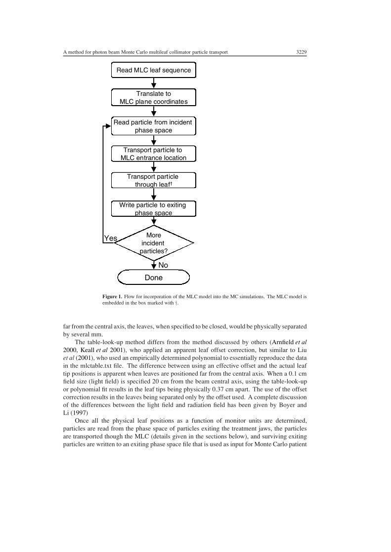
The general flow for incorporating the MLC model into MC dose calculation is shown infigure 1. The positions of the MLC leaves are read from the MLC leaf-sequence file thatis normally sent from the treatment-planning system to the treatment machine for use intreatment. This file specifies the projection of the MLC light field to 100-cm SAD at specifiedfractional monitor units of the total beam delivery (see the appendix for further discussion ofthe leaf-sequence file). The sequence of sub-fields in the file can result in static beam delivery,SMLC IMRT beam delivery, or DMLC IMRT beam delivery. The positions specified in theleaf-sequence file are translated into physical leaf coordinates using the same method asthe treatment machine. That is, they are translated to physical leaf tip positions at the MLCplane using a table-look-up and demagnification from the treatment machine mlctable.txt file.The table look-up accounts for the rounded leaf tip light projection to the isocentre plane whilethe demagnification projects the field to the MLC location. It is important to note that whenthe A (right) and B (left) leaves of an MLC pair are specified to be at the same position (thatis the leaf pair is specified to be closed), instead of using the positions directly from the tablelook-up, which could result in a physical gap between the leaves but no light field gap, bothleaves are positioned at the mean location from the table-look-up before the demagnificationis applied. This results in the leaves physically touching. If this were not the case, at distances

1 Varian Medical Systems, Palo Alto, CA 94304-1129.


Read MLC leaf sequence

Translate toMLC plane coordinates

Read particle from incident phase space

Transport particle to MLC entrance location

Transport particle through leaf†

Write particle to exiting phase space

Moreincident particles?

Done

No

Yes

Figure 1. Flow for incorporation of the MLC model into the MC simulations. The MLC model isembedded in the box marked with †.

far from the central axis, the leaves, when specified to be closed, would be physically separatedby several mm.

The table-look-up method differs from the method discussed by others (Arnfield et al2000, Keall et al 2001), who applied an apparent leaf offset correction, but similar to Liuet al (2001), who used an empirically determined polynomial to essentially reproduce the datain the mlctable.txt file. The difference between using an effective offset and the actual leaftip positions is apparent when leaves are positioned far from the central axis. When a 0.1 cmfield size (light field) is specified 20 cm from the beam central axis, using the table-look-upor polynomial fit results in the leaf tips being physically 0.37 cm apart. The use of the offsetcorrection results in the leaves being separated only by the offset used. A complete discussionof the differences between the light field and radiation field has been given by Boyer andLi (1997)

Once all the physical leaf positions as a function of monitor units are determined,particles are read from the phase space of particles exiting the treatment jaws, the particlesare transported though the MLC (details given in the sections below), and surviving exitingparticles are written to an exiting phase space file that is used as input for Monte Carlo patient


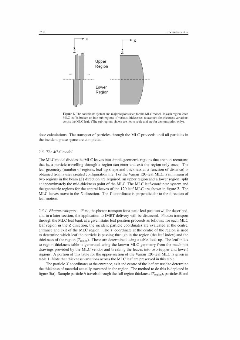
Figure 2. The coordinate system and major regions used for the MLC model. In each region, eachMLC leaf is broken up into sub-regions of various thicknesses to account for thickness variationsacross the MLC leaf. (The sub-regions shown are not to scale and are for demonstration only).

dose calculations. The transport of particles through the MLC proceeds until all particles inthe incident phase space are completed.

2.3. The MLC model

The MLC model divides the MLC leaves into simple geometric regions that are non-reentrant;that is, a particle travelling through a region can enter and exit the region only once. Theleaf geometry (number of regions, leaf tip shape and thickness as a function of distance) isobtained from a user created configuration file. For the Varian 120-leaf MLC, a minimum oftwo regions in the beam (Z) direction are required, an upper region and a lower region, splitat approximately the mid-thickness point of the MLC. The MLC leaf-coordinate system andthe geometric regions for the central leaves of the 120 leaf MLC are shown in figure 2. TheMLC leaves move in the X direction. The Y coordinate is perpendicular to the direction ofleaf motion.

2.3.1. Photon transport. First, the photon transport for a static leaf position will be described,and in a later section, the application to IMRT delivery will be discussed. Photon transportthrough the MLC leaf bank at a given static leaf position proceeds as follows: for each MLCleaf region in the Z direction, the incident particle coordinates are evaluated at the centre,entrance and exit of the MLC region. The Y coordinate at the centre of the region is usedto determine which leaf the particle is passing through in the region (the leaf index) and thethickness of the region (Tregion). These are determined using a table-look-up. The leaf indexto region thickness table is generated using the known MLC geometry from the machinistdrawings provided by the MLC vendor and breaking the leaves into two (upper and lower)regions. A portion of this table for the upper-section of the Varian 120-leaf MLC is given intable 1. Note that thickness variations across the MLC leaf are preserved in this table.

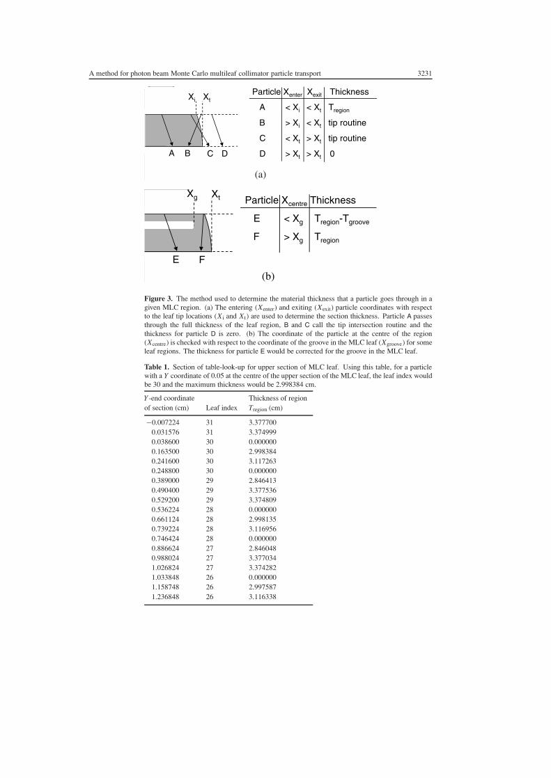
The particle X coordinates at the entrance, exit and centre of the leaf are used to determinethe thickness of material actually traversed in the region. The method to do this is depicted infigure 3(a). Sample particle A travels through the full region thickness (Tregion), particles B and


Particle Xenter Xexit Thickness

A < Xi < Xt Tregion

B > Xi < Xt tip routine

C < Xt > Xt tip routine

D > Xt > Xt 0A B

XtXi

C D

(a)

E F

XtXg Particle Xcentre Thickness

E < Xg Tregion-Tgroove

F > Xg Tregion

(b)

Figure 3. The method used to determine the material thickness that a particle goes through in agiven MLC region. (a) The entering (Xenter) and exiting (Xexit) particle coordinates with respectto the leaf tip locations (Xi and Xt) are used to determine the section thickness. Particle A passesthrough the full thickness of the leaf region, B and C call the tip intersection routine and thethickness for particle D is zero. (b) The coordinate of the particle at the centre of the region(Xcentre) is checked with respect to the coordinate of the groove in the MLC leaf (Xgroove) for someleaf regions. The thickness for particle E would be corrected for the groove in the MLC leaf.

Table 1. Section of table-look-up for upper section of MLC leaf. Using this table, for a particlewith a Y coordinate of 0.05 at the centre of the upper section of the MLC leaf, the leaf index wouldbe 30 and the maximum thickness would be 2.998384 cm.

Y -end coordinate Thickness of regionof section (cm) Leaf index Tregion (cm)

!0.007224 31 3.3777000.031576 31 3.3749990.038600 30 0.0000000.163500 30 2.9983840.241600 30 3.1172630.248800 30 0.0000000.389000 29 2.8464130.490400 29 3.3775360.529200 29 3.3748090.536224 28 0.0000000.661124 28 2.9981350.739224 28 3.1169560.746424 28 0.0000000.886624 27 2.8460480.988024 27 3.3770341.026824 27 3.3742821.033848 26 0.0000001.158748 26 2.9975871.236848 26 3.116338


G H

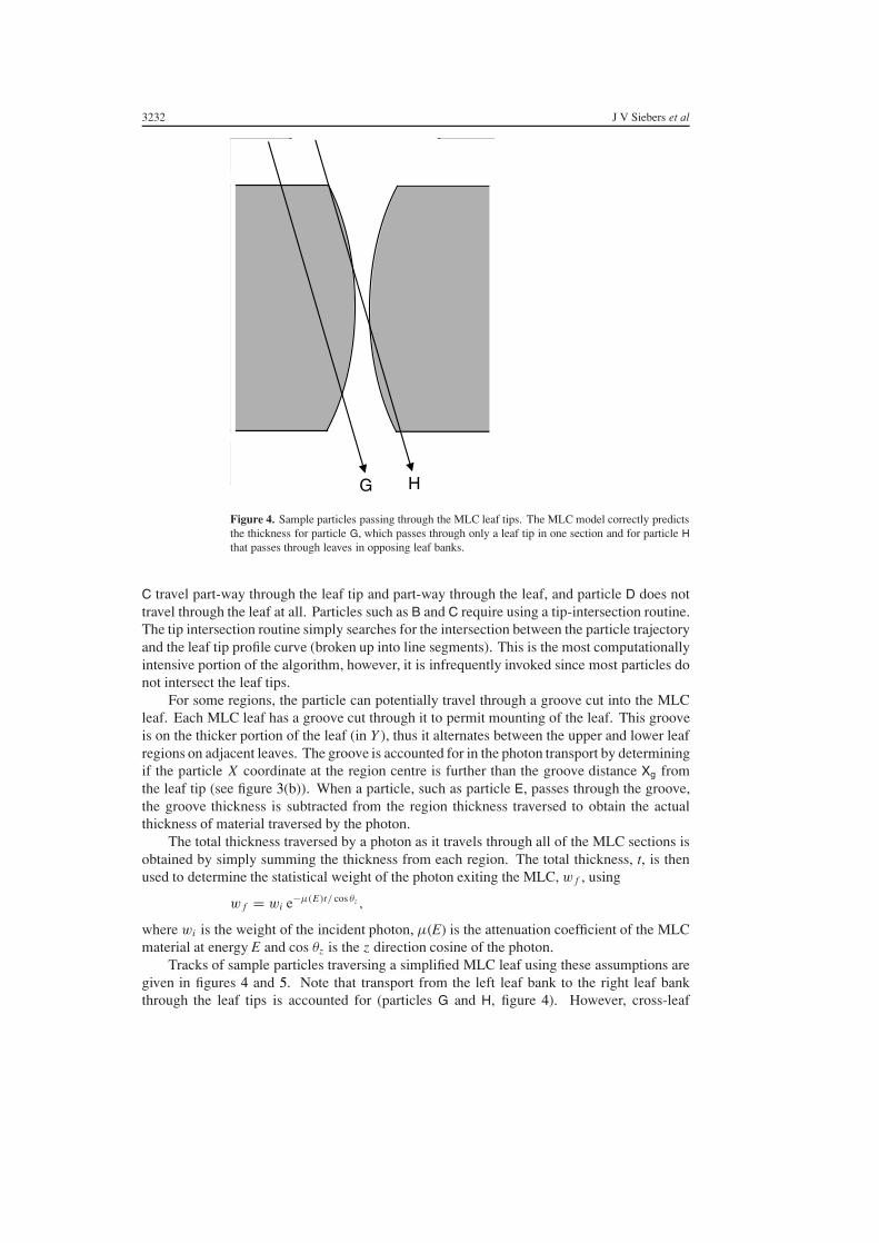
Figure 4. Sample particles passing through the MLC leaf tips. The MLC model correctly predictsthe thickness for particle G, which passes through only a leaf tip in one section and for particle Hthat passes through leaves in opposing leaf banks.

C travel part-way through the leaf tip and part-way through the leaf, and particle D does nottravel through the leaf at all. Particles such as B and C require using a tip-intersection routine.The tip intersection routine simply searches for the intersection between the particle trajectoryand the leaf tip profile curve (broken up into line segments). This is the most computationallyintensive portion of the algorithm, however, it is infrequently invoked since most particles donot intersect the leaf tips.

For some regions, the particle can potentially travel through a groove cut into the MLCleaf. Each MLC leaf has a groove cut through it to permit mounting of the leaf. This grooveis on the thicker portion of the leaf (in Y ), thus it alternates between the upper and lower leafregions on adjacent leaves. The groove is accounted for in the photon transport by determiningif the particle X coordinate at the region centre is further than the groove distance Xg fromthe leaf tip (see figure 3(b)). When a particle, such as particle E, passes through the groove,the groove thickness is subtracted from the region thickness traversed to obtain the actualthickness of material traversed by the photon.

The total thickness traversed by a photon as it travels through all of the MLC sections isobtained by simply summing the thickness from each region. The total thickness, t, is thenused to determine the statistical weight of the photon exiting the MLC, wf , using

wf = wi e!µ(E)t/ cos !z ,

where wi is the weight of the incident photon, µ(E) is the attenuation coefficient of the MLCmaterial at energy E and cos !z is the z direction cosine of the photon.

Tracks of sample particles traversing a simplified MLC leaf using these assumptions aregiven in figures 4 and 5. Note that transport from the left leaf bank to the right leaf bankthrough the leaf tips is accounted for (particles G and H, figure 4). However, cross-leaf


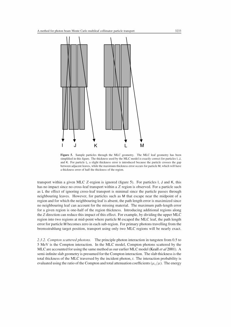
I J K L M

Figure 5. Sample particles through the MLC geometry. The MLC leaf geometry has beensimplified in this figure. The thickness used by the MLC model is exactly correct for particles I, J,and K. For particle L, a slight thickness error is introduced because the particle crosses the gapbetween adjacent leaves, while the maximum thickness error occurs for particle M, which will havea thickness error of half the thickness of the region.

transport within a given MLC Z-region is ignored (figure 5). For particles I, J and K, thishas no impact since no cross-leaf transport within a Z region is observed. For a particle suchas L the effect of ignoring cross-leaf transport is minimal since the particle passes throughneighbouring leaves. However, for particles such as M that escape near the midpoint of aregion and for which the neighbouring leaf is absent, the path length error is maximized sinceno neighbouring leaf can account for the missing material. The maximum path-length errorfor a given region is one-half of the region thickness. Introducing additional regions alongthe Z direction can reduce this impact of this effect. For example, by dividing the upper MLCregion into two regions at mid-point where particle M escaped the MLC leaf, the path lengtherror for particle M becomes zero in each sub-region. For primary photons travelling from thebremsstrahlung target position, transport using only two MLC regions will be nearly exact.

2.3.2. Compton scattered photons. The principle photon interaction in tungsten from 0.5 to5 MeV is the Compton interaction. In the MLC model, Compton photons scattered by theMLC are accounted for using the same method as our earlier MLC model (Keall et al 2001). Asemi-infinite slab geometry is presumed for the Compton interaction. The slab thickness is thetotal thickness of the MLC traversed by the incident photon, t. The interaction probability isevaluated using the ratio of the Compton and total attenuation coefficients (µc/µ). The energy


and angle of the Compton scattered photon are determined using the methods described inthe EGS4 user manuals (Nelson et al 1985). The location of the interaction as the photontraverses thickness t is randomly sampled over [0, t) assuming exponential attenuation. Thephase space coordinates of the scattered photon are used to determine the remaining thicknessto be traversed by the scattered photon (t "). The attenuation coefficient (µ"(E)), thickness (t "),and direction cosine (cos! "

z) are used to attenuate the scattered photon as it exits the materialslab. Thus, the weight of a scattered photon, w"

f , is

w"f = wi(1 ! e!µ(E)t/ cos !z )

µc

µe!µ(E")t "/ cos ! "

z .

Compton scattered electrons, photo-electrons, bremsstrahlung photons and pair productionproducts are ignored in this model.

2.3.3. Electron transport. Geometrically, electron transport through the MLC sections issimilar to the photon transport, however, the interest lies with whether the electrons intersectthe MLC leaves. If the electron intersects the MLC leaf or leaf tip, it is assigned zero weight.Otherwise, the electron travels through the MLC leaf opening with its weight unchanged.

2.3.4. Variance reduction techniques. To improve the efficiency of the later dose calculationalgorithm, Russian Roulette is performed on transmitted and scattered photons using themethod described in the MCNP manual. (Briesmeister 1997) That is, a statistical weightcut-off wcut is defined. Particles with a final weight wf above the weight cut-off survive withtheir statistical weight unchanged. Particles with wf less than wcut survive with a probabilityof wf /wcut. The weight of surviving particles is equal to wcut. The weight cut-off valueused for most calculations is 0.10, since the efficiency of delivering an IMRT field is typicallygreater than this value.

2.3.5. Application to IMRT. The above sections describe the use of the MLC model for astatic radiation field. In IMRT, either many static MLC positions may be specified to create thedesired intensity profile (SMLC IMRT) or the MLC leaves may be moving when the beam ison (DMLC IMRT). In either case, the MLC leaf-sequencing file specifies the positions of eachMLC leaf at specified fractional monitor units (MUs) of the total MUs. Between these MUindices, each MLC leaf travels linearly to the next position and fractional MU. (For SMLCIMRT, leaf travel occurs when different MLC positions are specified at the same number offractional MUs, and beam irradiation occurs when the same leaf position occurs at differentconsecutive fractional MU settings.) For a given arbitrary fractional MU, the positions of theA (right) and B (left) MLC leaves for the segment are determined by linear interpolation ofpositions specified in the MLC file.

As a variance reduction technique in this model, each particle is transported throughthe MLC at N randomly selected fractional MU positions. The MLC leaf positions maybe different at each of these different fractional MUs. At each fractional MU setting k, theentering and exiting X coordinates of the particle in each MLC region are used to determinethe total thickness the particle traversed at that fractional MU setting. The average statisticalweight of a particle exiting the MLC is the geometric mean of the weights from the individualfractional MU settings. That is, for photons

wf = wi

N

N!

k=1

e!µ(E)tk/ cos !z .


To further reduce computational burden, Compton events are sampled only once for eachincident photon rather than at each fractional MU setting. That is, one of the kth thicknesses(tk) is used to determine the Compton scatter event. Since the fractional MUs are chosenrandomly, the last fractional MU position is as random as any other and is used for determiningthe Compton scatter. This method preserves the mean number of scattered photons exiting theMLC. The default value of N is 100, and all of the calculations presented here used this value.

3. Benchmark tests and results

To benchmark the MLC model, results obtained with the model were compared withmeasurements and other MC calculations for a variety of test cases. Validation tests wereperformed using the 6 MV and 18 MV beams from our Varian 21EX linear accelerator with aMillenium 120 leaf MLC attached. Monte Carlo calculations were performed using the MCVMC system. Integration of the MC code with the treatment-planning system, generation ofinitial phase space, modelling of beam line devices and dose calculation have been describedelsewhere (Siebers 1999, Siebers et al 2000b).

3.1. Blocked field tests

Several test fields created with the MLC blocking the entire treatment field were used toestablish the ability of the MLC to correctly predict the attenuation and scatter characteristicsof the MLC. For these tests, the beam-defining jaws were set to produce a given field size, forexample, a 10 # 10 cm2 field at an SAD of 100 cm, but the MLC leaves extended across theradiation field, hence blocking the radiation field. We call such a field an MLC-blocked field.

3.1.1. Leakage as function of field size. Overall predictions of MLC leakage (transmitted +scattered) radiation were performed by comparing measurements with MC simulations formultiple MLC-blocked field sizes. Measurements of the radiation leakage through theMLC at a depth of 5 cm in a water equivalent phantom placed at 95 cm SSD weremade using a PTW Farmer-type ionization chamber (internal diameter 6.25 mm, length24.0 mm). Measurements were taken for open and MLC-blocked field sizes of 5 # 5,10 # 10, and 15 # 15 cm2. For the MLC-blocked fields, measurements were taken withthe A and B leaf banks blocking the field and averaged. The ion chamber was orientedperpendicular to the direction of leaf motion to average out the variable transmission throughthe leaves due to the thickness profile of the leaves. Measurements were taken with thechamber on the central axis and with the chamber offset by $±3 mm to ensure that dosevariations due to undulations in the leakage dose profile were properly averaged. At each fieldsize, MLC-blocked field results were normalized to the open-field measurements to obtainthe fractional MLC leakage. MC simulations were performed for conditions that reproducedthe experimental conditions. The MC calculations were performed using the MLC modeldescribed in this paper and using the full MLC geometry for an MCNP simulation. The fullMC simulation of the MLC is detailed in the paper by Kim et al (2001). The MCNP simulationincorporates all geometric aspects of the MLC-leaf design and includes full physics treatmentof photon and electron interactions. MCNP was used to transport only through the MLC.The EGS4 (Nelson et al 1985) BEAM user code (Rogers et al 1995) was used to transportthrough the other parts of the accelerator head and DOSXYZ (Ma et al 1995) was used fortransport through the phantom. A 0.6 # 0.6 # 1.0 cm3 voxel size was used during theMC transport simulations, however, the central five voxels in the direction orthogonal tothe beam were averaged to reduce statistical fluctuations, creating an effective voxel size of


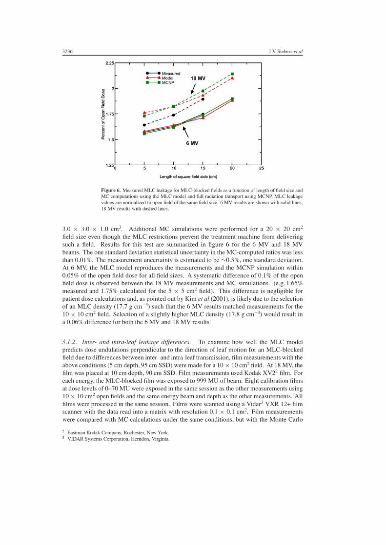
Figure 6. Measured MLC leakage for MLC-blocked fields as a function of length of field size andMC computations using the MLC model and full radiation transport using MCNP. MLC leakagevalues are normalized to open field of the same field size. 6 MV results are shown with solid lines,18 MV results with dashed lines.

3.0 # 3.0 # 1.0 cm3. Additional MC simulations were performed for a 20 # 20 cm2

field size even though the MLC restrictions prevent the treatment machine from deliveringsuch a field. Results for this test are summarized in figure 6 for the 6 MV and 18 MVbeams. The one standard deviation statistical uncertainty in the MC-computed ratios was lessthan 0.01%. The measurement uncertainty is estimated to be $0.3%, one standard deviation.At 6 MV, the MLC model reproduces the measurements and the MCNP simulation within0.05% of the open field dose for all field sizes. A systematic difference of 0.1% of the openfield dose is observed between the 18 MV measurements and MC simulations. (e.g. 1.65%measured and 1.75% calculated for the 5 # 5 cm2 field). This difference is negligible forpatient dose calculations and, as pointed out by Kim et al (2001), is likely due to the selectionof an MLC density (17.7 g cm!3) such that the 6 MV results matched measurements for the10 # 10 cm2 field. Selection of a slightly higher MLC density (17.8 g cm!3) would result ina 0.06% difference for both the 6 MV and 18 MV results.

3.1.2. Inter- and intra-leaf leakage differences. To examine how well the MLC modelpredicts dose undulations perpendicular to the direction of leaf motion for an MLC-blockedfield due to differences between inter- and intra-leaf transmission, film measurements with theabove conditions (5 cm depth, 95 cm SSD) were made for a 10 # 10 cm2 field. At 18 MV, thefilm was placed at 10 cm depth, 90 cm SSD. Film measurements used Kodak XV22 film. Foreach energy, the MLC-blocked film was exposed to 999 MU of beam. Eight calibration filmsat dose levels of 0–70 MU were exposed in the same session as the other measurements using10 # 10 cm2 open fields and the same energy beam and depth as the other measurements. Allfilms were processed in the same session. Films were scanned using a Vidar3 VXR 12+ filmscanner with the data read into a matrix with resolution 0.1 # 0.1 cm2. Film measurementswere compared with MC calculations under the same conditions, but with the Monte Carlo

2 Eastman Kodak Company, Rochester, New York.3 VIDAR Systems Corporation, Herndon, Virginia.


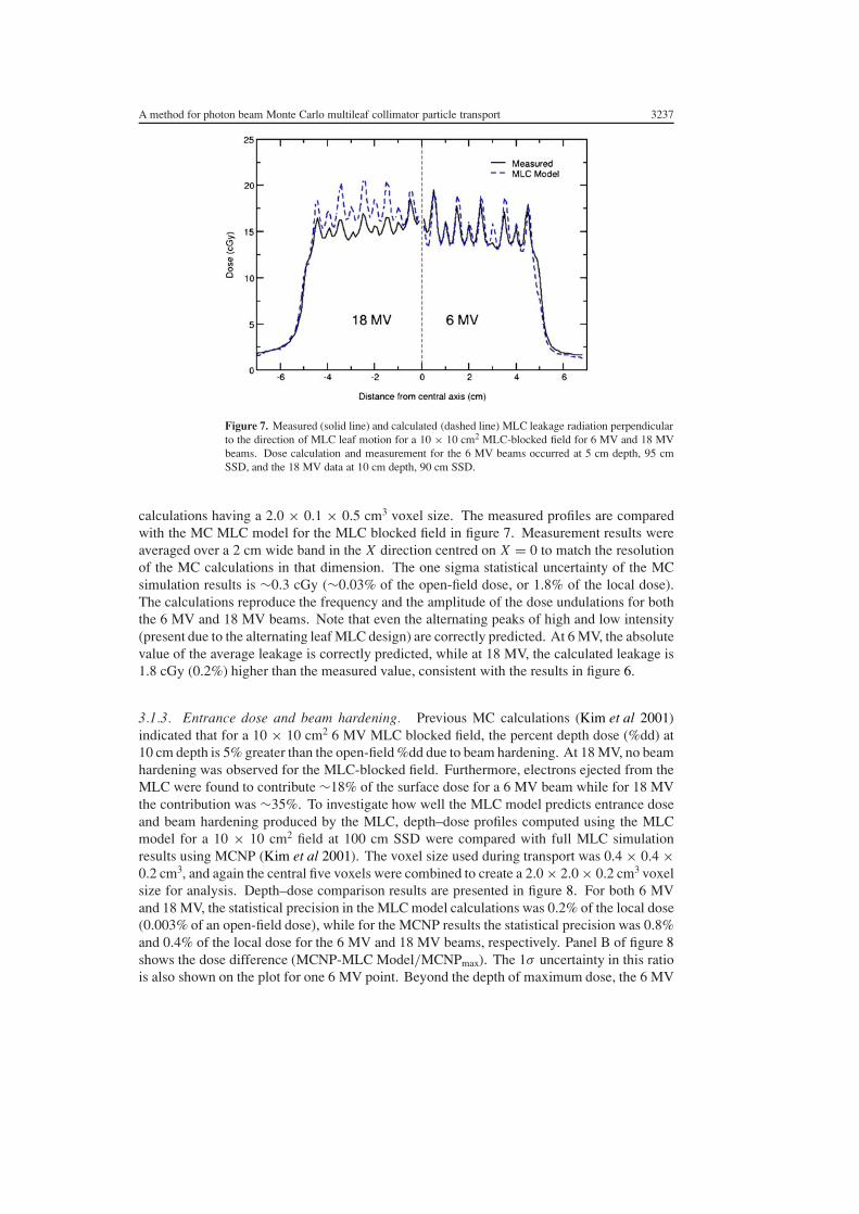
Figure 7. Measured (solid line) and calculated (dashed line) MLC leakage radiation perpendicularto the direction of MLC leaf motion for a 10 # 10 cm2 MLC-blocked field for 6 MV and 18 MVbeams. Dose calculation and measurement for the 6 MV beams occurred at 5 cm depth, 95 cmSSD, and the 18 MV data at 10 cm depth, 90 cm SSD.

calculations having a 2.0 # 0.1 # 0.5 cm3 voxel size. The measured profiles are comparedwith the MC MLC model for the MLC blocked field in figure 7. Measurement results wereaveraged over a 2 cm wide band in the X direction centred on X = 0 to match the resolutionof the MC calculations in that dimension. The one sigma statistical uncertainty of the MCsimulation results is $0.3 cGy ($0.03% of the open-field dose, or 1.8% of the local dose).The calculations reproduce the frequency and the amplitude of the dose undulations for boththe 6 MV and 18 MV beams. Note that even the alternating peaks of high and low intensity(present due to the alternating leaf MLC design) are correctly predicted. At 6 MV, the absolutevalue of the average leakage is correctly predicted, while at 18 MV, the calculated leakage is1.8 cGy (0.2%) higher than the measured value, consistent with the results in figure 6.

3.1.3. Entrance dose and beam hardening. Previous MC calculations (Kim et al 2001)indicated that for a 10 # 10 cm2 6 MV MLC blocked field, the percent depth dose (%dd) at10 cm depth is 5% greater than the open-field %dd due to beam hardening. At 18 MV, no beamhardening was observed for the MLC-blocked field. Furthermore, electrons ejected from theMLC were found to contribute $18% of the surface dose for a 6 MV beam while for 18 MVthe contribution was $35%. To investigate how well the MLC model predicts entrance doseand beam hardening produced by the MLC, depth–dose profiles computed using the MLCmodel for a 10 # 10 cm2 field at 100 cm SSD were compared with full MLC simulationresults using MCNP (Kim et al 2001). The voxel size used during transport was 0.4 # 0.4 #0.2 cm3, and again the central five voxels were combined to create a 2.0 # 2.0 # 0.2 cm3 voxelsize for analysis. Depth–dose comparison results are presented in figure 8. For both 6 MVand 18 MV, the statistical precision in the MLC model calculations was 0.2% of the local dose(0.003% of an open-field dose), while for the MCNP results the statistical precision was 0.8%and 0.4% of the local dose for the 6 MV and 18 MV beams, respectively. Panel B of figure 8shows the dose difference (MCNP-MLC Model/MCNPmax). The 1" uncertainty in this ratiois also shown on the plot for one 6 MV point. Beyond the depth of maximum dose, the 6 MV


0.02

0.015

0.01

0.005

00 5 10 15 20 25 30

0 5 10 15 20 25 30

18 MV

6 MV

Depth (cm)

Dos

e pe

r M

U (c

Gy/

MU

)P

erce

nt D

iffer

ence

6

5

4

3

2

1

0

-1

-2

-3

-4

-5

Depth (cm)

(a)

(b)

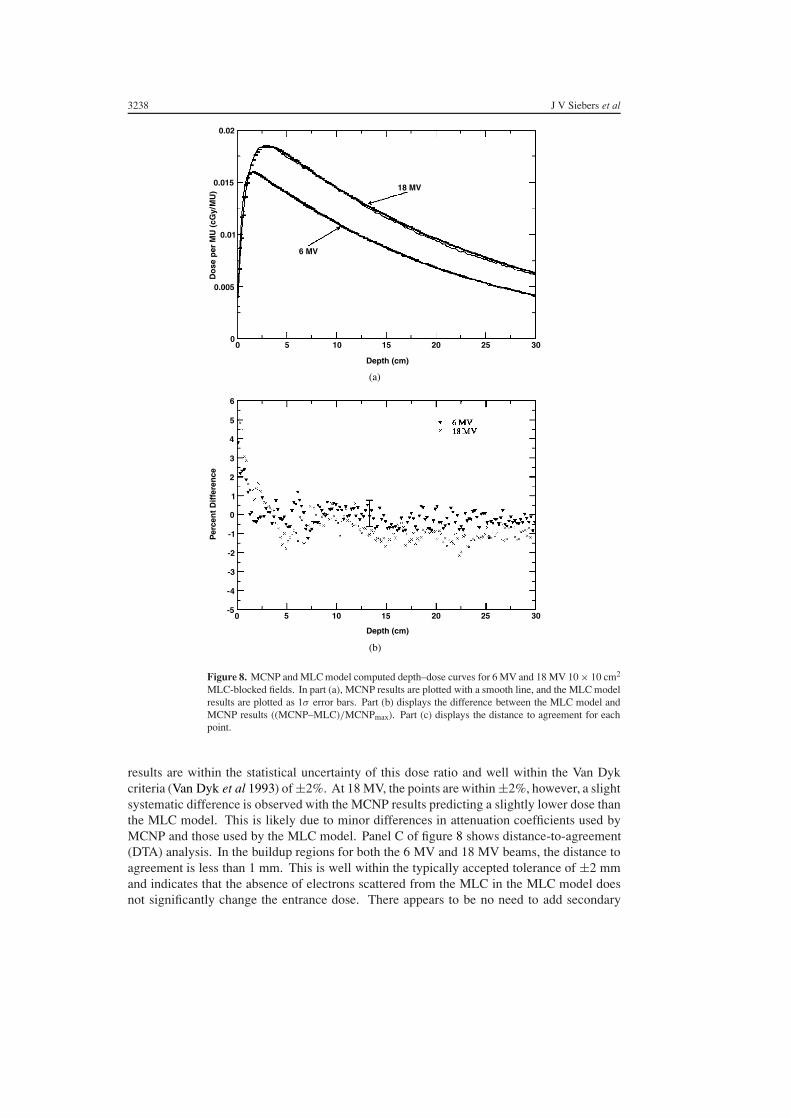
Figure 8. MCNP and MLC model computed depth–dose curves for 6 MV and 18 MV 10 # 10 cm2

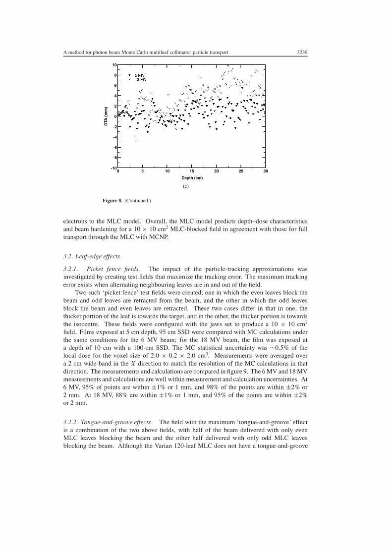
MLC-blocked fields. In part (a), MCNP results are plotted with a smooth line, and the MLC modelresults are plotted as 1" error bars. Part (b) displays the difference between the MLC model andMCNP results ((MCNP–MLC)/MCNPmax). Part (c) displays the distance to agreement for eachpoint.

results are within the statistical uncertainty of this dose ratio and well within the Van Dykcriteria (Van Dyk et al 1993) of ±2%. At 18 MV, the points are within ±2%, however, a slightsystematic difference is observed with the MCNP results predicting a slightly lower dose thanthe MLC model. This is likely due to minor differences in attenuation coefficients used byMCNP and those used by the MLC model. Panel C of figure 8 shows distance-to-agreement(DTA) analysis. In the buildup regions for both the 6 MV and 18 MV beams, the distance toagreement is less than 1 mm. This is well within the typically accepted tolerance of ±2 mmand indicates that the absence of electrons scattered from the MLC in the MLC model doesnot significantly change the entrance dose. There appears to be no need to add secondary


0 5 10 15 20 25 30

DTA

(mm

)

10

8

6

4

2

0

-2

-4

-6

-8

-10

Depth (cm)

(c)

Figure 8. (Continued.)

electrons to the MLC model. Overall, the MLC model predicts depth–dose characteristicsand beam hardening for a 10 # 10 cm2 MLC-blocked field in agreement with those for fulltransport through the MLC with MCNP.

3.2. Leaf-edge effects

3.2.1. Picket fence fields. The impact of the particle-tracking approximations wasinvestigated by creating test fields that maximize the tracking error. The maximum trackingerror exists when alternating neighbouring leaves are in and out of the field.

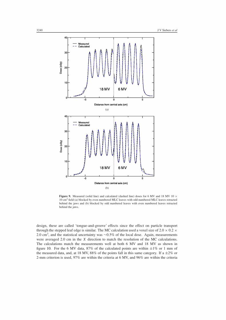
Two such ‘picket fence’ test fields were created; one in which the even leaves block thebeam and odd leaves are retracted from the beam, and the other in which the odd leavesblock the beam and even leaves are retracted. These two cases differ in that in one, thethicker portion of the leaf is towards the target, and in the other, the thicker portion is towardsthe isocentre. These fields were configured with the jaws set to produce a 10 # 10 cm2

field. Films exposed at 5 cm depth, 95 cm SSD were compared with MC calculations underthe same conditions for the 6 MV beam; for the 18 MV beam, the film was exposed ata depth of 10 cm with a 100-cm SSD. The MC statistical uncertainty was $0.5% of thelocal dose for the voxel size of 2.0 # 0.2 # 2.0 cm3. Measurements were averaged overa 2 cm wide band in the X direction to match the resolution of the MC calculations in thatdirection. The measurements and calculations are compared in figure 9. The 6 MV and 18 MVmeasurements and calculations are well within measurement and calculation uncertainties. At6 MV, 95% of points are within ±1% or 1 mm, and 98% of the points are within ±2% or2 mm. At 18 MV, 88% are within ±1% or 1 mm, and 95% of the points are within ±2%or 2 mm.

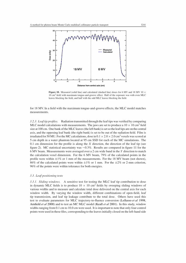
3.2.2. Tongue-and-groove effects. The field with the maximum ‘tongue-and-groove’ effectis a combination of the two above fields, with half of the beam delivered with only evenMLC leaves blocking the beam and the other half delivered with only odd MLC leavesblocking the beam. Although the Varian 120-leaf MLC does not have a tongue-and-groove


(b)

(a)

40

30

20

10

0

40

30

20

10

0-5 0 5

-5 0 5

Figure 9. Measured (solid line) and calculated (dashed line) doses for 6 MV and 18 MV 10 #10 cm2 field (a) blocked by even numbered MLC leaves with odd numbered MLC leaves retractedbehind the jaws and (b) blocked by odd numbered leaves with even numbered leaves retractedbehind the jaws.

design, these are called ‘tongue-and-groove’ effects since the effect on particle transportthrough the stepped leaf edge is similar. The MC calculation used a voxel size of 2.0 # 0.2 #2.0 cm3, and the statistical uncertainty was $0.5% of the local dose. Again, measurementswere averaged 2.0 cm in the X direction to match the resolution of the MC calculations.The calculations match the measurements well at both 6 MV and 18 MV as shown infigure 10. For the 6 MV data, 87% of the calculated points are within ±1% or 1 mm ofthe measured data, and, at 18 MV, 88% of the points fall in this same category. If a ±2% or2-mm criterion is used, 97% are within the criteria at 6 MV, and 96% are within the criteria


50

40

30

20

10

0-6 -4 -2 0 2 4 6

Figure 10. Measured (solid line) and calculated (dashed line) doses for 6 MV and 18 MV 10 #10 cm2 field with maximum tongue-and-groove effect. Half of the exposure was with even MLCleaves blocking the field, and half with the odd MLC leaves blocking the field.

for 18 MV. In a field with the maximum tongue-and-groove effects, the MLC model matchesmeasurements.

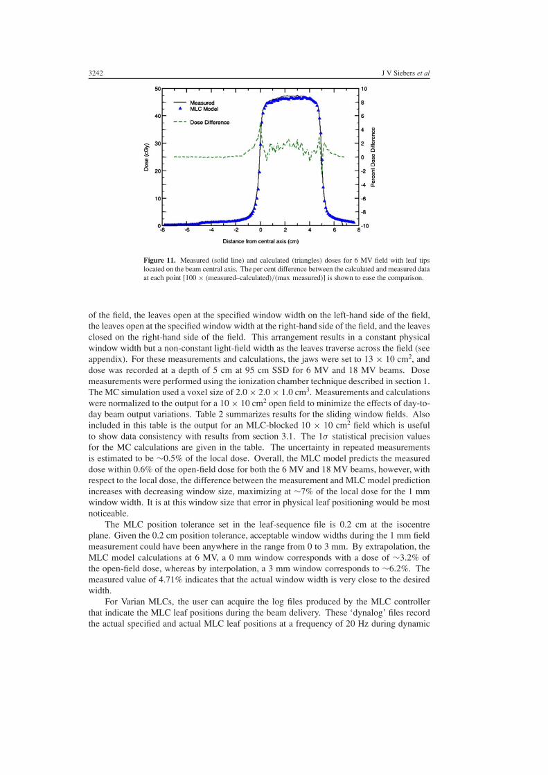
3.2.3. Leaf tip profiles. Radiation transmitted through the leaf tips was verified by comparingMLC model calculations with measurements. The jaws are set to produce a 10 # 10 cm2 fieldsize at 100 cm. One bank of the MLC leaves (the left bank) is set so the leaf tips are on the centralaxis, and the opposing leaf bank (the right bank) is set to be out of the radiation field. Film isirradiated for 50 MU. For the MC calculations, dose in 0.1 # 2.0 # 2.0 cm3 voxels was scored at5 cm depth in a water phantom located at 95 cm SSD for each of the MC simulations. The0.1 cm dimension for the profile is along the X direction, the direction of the leaf tip (seefigure 2). MC statistical uncertainty was $0.3%. Results are compared in figure 11 for the6 MV beam. Measurements were averaged over a 2 cm wide band in the Y direction to matchthe calculation voxel dimension. For the 6 MV beam, 79% of the calculated points in theprofile were within ±1% or 1 mm of the measurements. For the 18 MV beam (not shown),86% of the calculated points were within ±1% or 1 mm. For the ±2% or 2-mm criterion,96% of the points were within tolerance for both energies.

3.3. Leaf-positioning tests

3.3.1. Sliding windows. A sensitive test for testing the MLC leaf tip contribution to dosein dynamic MLC fields is to produce 10 # 10 cm2 fields by sweeping sliding windows ofvarious widths and to measure and calculate total dose delivered on the central axis for eachwindow width. By varying the window width, different combinations of open-field, leaftip transmission, and leaf tip leakage contribute to the total dose. Others have used thistest to evaluate parameters for MLC trajectory-to-fluence conversion (LoSasso et al 1998,Arnfield et al 2000) and to test an MC MLC model (Keall et al 2001). In this study, windowwidths ranging from 0.1 cm to 10.0 cm were used. It is important to note that only four controlpoints were used in these files, corresponding to the leaves initially closed on the left-hand side


Figure 11. Measured (solid line) and calculated (triangles) doses for 6 MV field with leaf tipslocated on the beam central axis. The per cent difference between the calculated and measured dataat each point [100 # (measured–calculated)/(max measured)] is shown to ease the comparison.

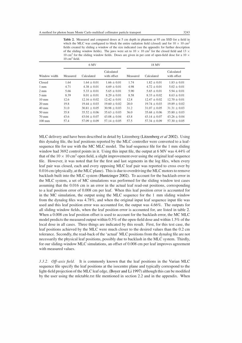
of the field, the leaves open at the specified window width on the left-hand side of the field,the leaves open at the specified window width at the right-hand side of the field, and the leavesclosed on the right-hand side of the field. This arrangement results in a constant physicalwindow width but a non-constant light-field width as the leaves traverse across the field (seeappendix). For these measurements and calculations, the jaws were set to 13 # 10 cm2, anddose was recorded at a depth of 5 cm at 95 cm SSD for 6 MV and 18 MV beams. Dosemeasurements were performed using the ionization chamber technique described in section 1.The MC simulation used a voxel size of 2.0 # 2.0 # 1.0 cm3. Measurements and calculationswere normalized to the output for a 10 # 10 cm2 open field to minimize the effects of day-to-day beam output variations. Table 2 summarizes results for the sliding window fields. Alsoincluded in this table is the output for an MLC-blocked 10 # 10 cm2 field which is usefulto show data consistency with results from section 3.1. The 1" statistical precision valuesfor the MC calculations are given in the table. The uncertainty in repeated measurementsis estimated to be $0.5% of the local dose. Overall, the MLC model predicts the measureddose within 0.6% of the open-field dose for both the 6 MV and 18 MV beams, however, withrespect to the local dose, the difference between the measurement and MLC model predictionincreases with decreasing window size, maximizing at $7% of the local dose for the 1 mmwindow width. It is at this window size that error in physical leaf positioning would be mostnoticeable.

The MLC position tolerance set in the leaf-sequence file is 0.2 cm at the isocentreplane. Given the 0.2 cm position tolerance, acceptable window widths during the 1 mm fieldmeasurement could have been anywhere in the range from 0 to 3 mm. By extrapolation, theMLC model calculations at 6 MV, a 0 mm window corresponds with a dose of $3.2% ofthe open-field dose, whereas by interpolation, a 3 mm window corresponds to $6.2%. Themeasured value of 4.71% indicates that the actual window width is very close to the desiredwidth.

For Varian MLCs, the user can acquire the log files produced by the MLC controllerthat indicate the MLC leaf positions during the beam delivery. These ‘dynalog’ files recordthe actual specified and actual MLC leaf positions at a frequency of 20 Hz during dynamic


Table 2. Measured and computed doses at 5 cm depth in phantom at 95 cm SSD for a field inwhich the MLC was configured to block the entire radiation field (closed) and for 10 # 10 cm2

fields created by sliding a window of the size indicated (see the appendix for further descriptionof the sliding window fields). The jaws were set to 10 # 10 cm2 for the closed field and 13 #10 cm2 for the sliding window fields. Doses are given in per cent of open-field dose for a 10 #10 cm2 field.

6 MV 18 MV

Calculated CalculatedWindow width Measured Calculated with offset Measured Calculated with offset

Closed 1.64 1.64 ± 0.01 1.66 ± 0.01 1.74 1.82 ± 0.01 1.83 ± 0.011 mm 4.71 4.38 ± 0.01 4.69 ± 0.01 4.98 4.72 ± 0.01 5.02 ± 0.012 mm 5.66 5.33 ± 0.01 5.65 ± 0.01 5.90 5.65 ± 0.01 5.94 ± 0.015 mm 8.39 8.01 ± 0.01 8.29 ± 0.01 8.58 8.33 ± 0.02 8.63 ± 0.0110 mm 12.6 12.16 ± 0.02 12.42 ± 0.01 12.8 12.47 ± 0.02 12.70 ± 0.0120 mm 19.8 19.44 ± 0.03 19.60 ± 0.02 20.0 19.74 ± 0.03 19.89 ± 0.0240 mm 31.0 30.81 ± 0.05 30.98 ± 0.03 31.2 31.07 ± 0.05 31.31 ± 0.0350 mm 35.8 35.52 ± 0.06 35.63 ± 0.03 36.0 35.68 ± 0.06 35.80 ± 0.0370 mm 43.6 43.04 ± 0.07 43.08 ± 0.04 43.8 43.14 ± 0.07 43.26 ± 0.04100 mm 57.4 57.09 ± 0.09 57.14 ± 0.05 57.5 57.34 ± 0.09 57.30 ± 0.05

MLC delivery and have been described in detail by Litzenberg (Litzenberg et al 2002). Usingthis dynalog file, the leaf positions reported by the MLC controller were converted to a leaf-sequence file for use with the MC MLC model. The leaf-sequence file for the 1 mm slidingwindow had 3692 control points in it. Using this input file, the output at 6 MV was 4.44% ofthat of the 10 # 10 cm2 open field, a slight improvement over using the original leaf-sequencefile. However, it was noted that for the first and last segments in the log files, when everyleaf pair was closed, each and every opposing MLC leaf pair was reported to cross over by0.016 cm (physically, at the MLC plane). This is due to overdriving the MLC motors to removebacklash built into the MLC system (Huntzinger 2002). To account for the backlash error inthe MLC system, a set of MC simulations was performed for the sliding window test casesassuming that the 0.016 cm is an error in the actual leaf read-out positions, correspondingto a leaf position error of 0.008 cm per leaf. When this leaf position error is accounted forin the MC simulation, the output using the MLC sequence for the 1 mm sliding windowfrom the dynalog files was 4.78%, and when the original input leaf sequence input file wasused and this leaf position error was accounted for, the output was 4.66%. The outputs forall sliding window fields, when the leaf position error is accounted for, are listed in table 2.When a 0.008 cm leaf position offset is used to account for the backlash error, the MC MLCmodel predicts the measured output within 0.5% of the open-field dose and within 1.5% of thelocal dose in all cases. Three things are indicated by this result. First, for this test case, theleaf positions achieved by the MLC were much closer to the desired values than the 0.2 cmtolerance. Secondly, the read-back of the ‘actual’ MLC positions from the dynalog file are notnecessarily the physical leaf positions, possibly due to backlash in the MLC system. Thirdly,for our sliding-window MLC simulations, an offset of 0.008 cm per leaf improves agreementwith measured values.

3.3.2. Off–axis field. It is commonly known that the leaf positions in the Varian MLCsequence file specify the leaf positions at the isocentre plane and typically correspond to thelight-field projection of the MLC leaf edge, (Boyer and Li 1997) although this can be modifiedby the user using the mlctable.txt file mentioned in section 2.2 and in the appendix. When


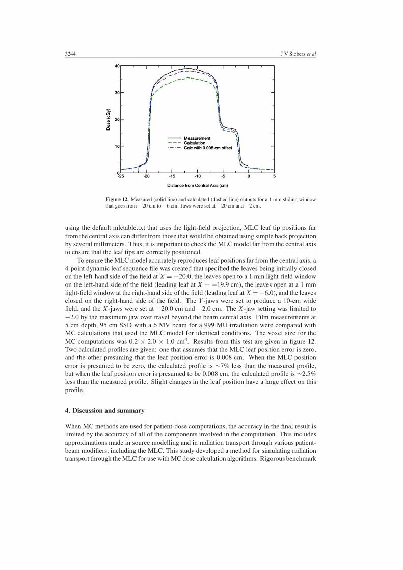
Figure 12. Measured (solid line) and calculated (dashed line) outputs for a 1 mm sliding windowthat goes from !20 cm to !6 cm. Jaws were set at !20 cm and !2 cm.

using the default mlctable.txt that uses the light-field projection, MLC leaf tip positions farfrom the central axis can differ from those that would be obtained using simple back projectionby several millimeters. Thus, it is important to check the MLC model far from the central axisto ensure that the leaf tips are correctly positioned.

To ensure the MLC model accurately reproduces leaf positions far from the central axis, a4-point dynamic leaf sequence file was created that specified the leaves being initially closedon the left-hand side of the field at X = !20.0, the leaves open to a 1 mm light-field windowon the left-hand side of the field (leading leaf at X = !19.9 cm), the leaves open at a 1 mmlight-field window at the right-hand side of the field (leading leaf at X = !6.0), and the leavesclosed on the right-hand side of the field. The Y -jaws were set to produce a 10-cm widefield, and the X-jaws were set at !20.0 cm and !2.0 cm. The X-jaw setting was limited to!2.0 by the maximum jaw over travel beyond the beam central axis. Film measurements at5 cm depth, 95 cm SSD with a 6 MV beam for a 999 MU irradiation were compared withMC calculations that used the MLC model for identical conditions. The voxel size for theMC computations was 0.2 # 2.0 # 1.0 cm3. Results from this test are given in figure 12.Two calculated profiles are given: one that assumes that the MLC leaf position error is zero,and the other presuming that the leaf position error is 0.008 cm. When the MLC positionerror is presumed to be zero, the calculated profile is $7% less than the measured profile,but when the leaf position error is presumed to be 0.008 cm, the calculated profile is $2.5%less than the measured profile. Slight changes in the leaf position have a large effect on thisprofile.

4. Discussion and summary

When MC methods are used for patient-dose computations, the accuracy in the final result islimited by the accuracy of all of the components involved in the computation. This includesapproximations made in source modelling and in radiation transport through various patient-beam modifiers, including the MLC. This study developed a method for simulating radiationtransport through the MLC for use with MC dose calculation algorithms. Rigorous benchmark


tests were used to quantify the accuracy of the MLC model. One strength of the MLC modelis that is uses the same method as the treatment machine to determine the MLC leaf positionsas a function of the number of monitor units delivered.

One goal of the MLC model was that it be substantially faster than simulations usinga standard MC code with full physics treatment. Using the MLC-blocked field depth–dosetest case, in which both MCNP and MLC model calculations were performed, we foundthat the MLC model was 200 times faster than MCNP for the same problem on the samecomputer processor. A particle transport rate of 10,000–20,000 photons/second is achievedon 500 MHz Pentium III processors. The MLC model thus has met the goal of being reasonablyfast. Since the probability of a given photon interacting in the MLC is evaluated at multiplerandom fractional monitor units during the beam delivery to determine the average attenuationprobability, the model is also efficient.

Tests with the MLC blocking the radiation field indicate that the physics included inthe MLC model is sufficient. MLC-blocked fields will contribute the maximum amount ofelectron scatter from the MLC, have the maximum amount of bremsstrahlung interactions fromelectrons incident upon the MLC, and have the maximum amount of pair production fromphoton interactions in the MLC. Although the MLC model neglects each of these interactions,it accurately predicts the surface dose, beam hardening, and field size dependence of theleakage radiation from the MLC. This suggests that modelling only photon attenuation andfirst Compton scatter may be sufficient for other upstream beam modifiers without affectingthe final MC dose calculation result, particularly those modifiers located upstream of the MLClocation such as the jaws or upper wedges.

The tests with sliding windows of various widths indicate the ability of the MLC modelto accurately integrate the dose delivery from the closed, leaf tip, and open portions of DMLCbeam delivery. This accuracy is obtained because the MLC motion is modelled using the sametechnique as that used to control the MLC on the accelerator. Because the MLC leaf positionshave some position uncertainty due to backlash, sliding a small ($1 mm or less) window widthacross the field can be used to determine the magnitude of this position uncertainty. Inclusionof a physical leaf position error to account for backlash in the MLC simulation had a largereffect on the results than using the leaf positions reported in the MLC controller-produceddynalog files, even though the leaf position tolerance specified in the input files used in thisstudy was 0.2 cm. The leaf position error determined in this study (0.008 cm) is of littleconsequence for typical, clinically used window widths of 0.5 cm and greater. Furthermore,the backlash position error likely depends on the prior history of the leaf motion. However,given the sensitivity of the output to the leaf position error for small sliding windows, use ofa $1 mm sliding window field in routine MLC quality assurance would be a good way ofverifying the stability of the MLC.

The ability of the MLC model to correctly predict the dose undulations in MLC-blockedfields, the dose for picket-fence fields, and the dose in instances with the maximum tongue-and-groove effect indicate that the geometry simplifications made by the MLC model areinconsequential at the 1% dose level for test cases that most severely test the model. Inroutine clinical cases where leaves are at least partially synchronized, the effects of theseapproximations will be even less.

Overall, the MLC model developed has been shown to reproduce dose measurementsgenerally within ±1% or 1 mm. The MLC model is fast and efficient, and is applicable toand has been used for static beam, DMLC and SMLC IMRT beam deliveries. This model willbe useful for inclusion in MC-based IMRT dose calculations, for pre-treatment verificationof IMRT beam delivery, and for calculation of portal imager transmission images for patienttreatment verification.


5. Information

The source code for the MLC model described in this study and the MLC leaf sequence filesused in this study are available on request from the first author.

Acknowledgments

This work was supported by grants CA74043 and CA74158 from the National Cancer Institute.The authors would like to thank Varian Oncology Systems for providing information forMC modelling of the accelerator and MLC, and for supporting research efforts at VirginiaCommonwealth University. We would like to thank Chris Bartee for assistance with MLCmeasurements and providing ready answers to our questions about the MLC, Devon Murphyfor her meticulous editing of our manuscripts, and Jim Satterthwaite of Phillips MedicalSystems for providing us with the EGS4-based Compton scattering routines in C.

Appendix A. Control of Varian MLCs

Accurate modelling of the motion of the MLC during dynamic delivery is crucial for conversionof leaf motions to ‘deliverable’ intensities for conventional dose calculation and for MCsimulations that incorporate the MLC motion. Unfortunately, the literature is not clear inits description of MLC motion for Varian MLCs. This appendix discusses this motion. Thediscussion will first cover a single static MLC field and then expanded to cover DMLC andSMLC beam deliveries. The discussion will be given in the context of the 120 leaf MLC usedin this study, but, according to Varian documentation (2000), will equally apply to the 80 leafand 52 leaf MLCs.

The MLC consists of 120 MLC leaves. These leaves are contained in two leaf bankstermed the A- and B-leaf banks; thus there are 60 leaves in each leaf bank. A leaf pair consistsof leaves with the same index in A and B leaf banks. For static beam delivery, the position ofeach MLC leaf is contained in a computer file (a .mlc file). The MLC controller interprets theMLC positions from this file for each leaf pair as follows: For a given leaf pair, the positionsof the A and B leaves are read from the file. A table-look-up is performed from a file calledmlctable.txt to transform the positions indicated in the file to leaf tip positions. Note that ifthe specified position of the A leaf is the same as that of the B leaf (that is A leaf = !Bleaf, the leaves touching) then the mean position for the A and B leaves is determined fromthe mlctable.txt look-up, and both leaves are set to this same position. This keeps the MLCleaves touching when the leaf pair is specified to be closed. A demagnification of the A andB leaf positions to the MLC plane is then performed using a demagnification factor specifiedin the mlctable.txt file. The default mlctable.txt provided by Varian is configured such thatthe light-field projection of the rounded leaf tip will be at the position indicated in the leafposition file. This has been discussed at length by Boyer and Li (1997). It is possible for theuser to modify the mlctable.txt so that some other quantity is projected to the isocentre plane,such as the 50% isodose line, however, this is not recommended.

For DMLC and SMLC beam deliveries, the MLC motion is specified in a dynamic leaf-sequence file (.dml or .dma file). This format of this file is similar to that of the .mlc file exceptthat MLC positions are listed at various control points. At each control point, the fractionalnumber of monitor units (MU) [0,1] is also listed. The leaf positions at these control pointsare converted to the MLC plane using the same method as for static fields.

For dynamic delivery, for MU values between those indicated in the leaf-sequence file,the leaf positions are linearly interpolated. This interpolation occurs on the leaf positions after


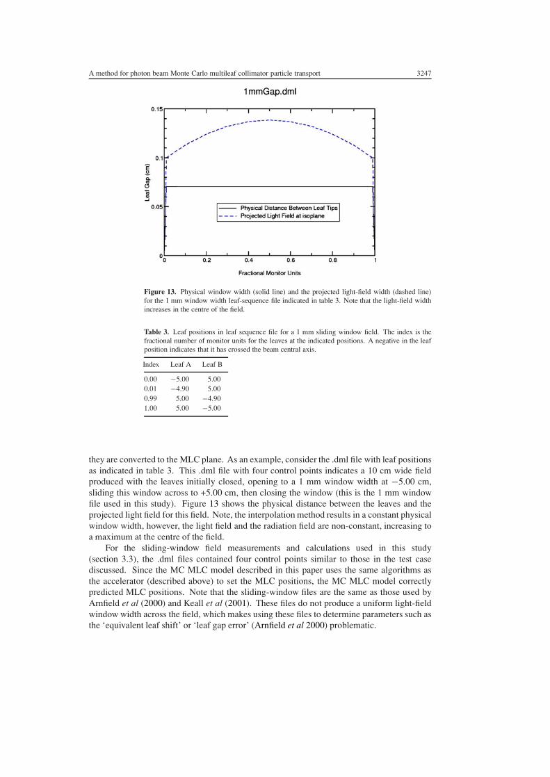
Figure 13. Physical window width (solid line) and the projected light-field width (dashed line)for the 1 mm window width leaf-sequence file indicated in table 3. Note that the light-field widthincreases in the centre of the field.

Table 3. Leaf positions in leaf sequence file for a 1 mm sliding window field. The index is thefractional number of monitor units for the leaves at the indicated positions. A negative in the leafposition indicates that it has crossed the beam central axis.

Index Leaf A Leaf B

0.00 !5.00 5.000.01 !4.90 5.000.99 5.00 !4.901.00 5.00 !5.00

they are converted to the MLC plane. As an example, consider the .dml file with leaf positionsas indicated in table 3. This .dml file with four control points indicates a 10 cm wide fieldproduced with the leaves initially closed, opening to a 1 mm window width at !5.00 cm,sliding this window across to +5.00 cm, then closing the window (this is the 1 mm windowfile used in this study). Figure 13 shows the physical distance between the leaves and theprojected light field for this field. Note, the interpolation method results in a constant physicalwindow width, however, the light field and the radiation field are non-constant, increasing toa maximum at the centre of the field.

For the sliding-window field measurements and calculations used in this study(section 3.3), the .dml files contained four control points similar to those in the test casediscussed. Since the MC MLC model described in this paper uses the same algorithms asthe accelerator (described above) to set the MLC positions, the MC MLC model correctlypredicted MLC positions. Note that the sliding-window files are the same as those used byArnfield et al (2000) and Keall et al (2001). These files do not produce a uniform light-fieldwindow width across the field, which makes using these files to determine parameters such asthe ‘equivalent leaf shift’ or ‘leaf gap error’ (Arnfield et al 2000) problematic.


References

Arnfield M R, Siebers J V, Kim J O, Wu Q, Keall P J and Mohan R 2000 A method for determining multileafcollimator transmission and scatter for dynamic intensity modulated radiotherapy Med. Phys. 27 2231–41

Balog J P, Mackie T R, Wenman D L, Glass M, Fang G and Pearson D 1999 Multileaf collimator interleaf transmissionMed. Phys. 26 176–86

Boyer A L and Li S 1997 Geometric analysis of light-field position of a multileaf collimator with curved ends Med.Phys. 24 757–62

Briesmeister J F 1997 MCNP—A general Monte Carlo N-particle transport code, version 4B Report LA-13181 (LosAlamos, NM: Los Alamos National Laboratory)

Chen Y, Boyer A L and Ma C M 2000 Calculation of x-ray transmission through a multileaf collimator Med. Phys.27 1717–26

Convery D J and Rosenbloom M E 1992 The generation of intensity-modulated fields for conformal radiotherapy bydynamic collimation Phys. Med. Biol. 37 1359–74

Convery D and Webb S 1997 Calculation of the distribution of head-scattered radiation in dynamically-collimatedMLC fields XIIth ICCR (Salt Lake City, UT, 27–30 May, 1997) pp 350–3

Deng J, Pawlicki T, Chen Y, Li J, Jiang S B and Ma C M 2001 The MLC tongue-and-groove effect on IMRT dosedistributions Phys. Med. Biol. 46 1039–60

Dirkx M L, Heijmen B J and van Santvoort J P 1998 Leaf trajectory calculation for dynamic multileaf collimation torealize optimized fluence profiles Phys. Med. Biol. 43 1171–84

Fix M K, Manser P, Born E J, Mini R and Ruegsegger P 2001a Monte Carlo simulation of a dynamic MLC based ona multiple source model Phys. Med. Biol. 46 3241–57

Fix M K, Manser P, Born E J, Vetterli D, Mini R and Ruegsegger P 2001b Monte Carlo simulation of a dynamicMLC: implementation and applications Z. Med. Phys. 11 163–70

Huntzinger C 2002 Personal communicationJeraj R and Keall P 1999 Monte Carlo-based inverse treatment planning Phys. Med. Biol. 44 1885–96Kapur A, Ma C M and Boyer A L 2000 Monte Carlo simulations for multileaf collimator leaves: design and dosimetry

2000 World Congress on Medical Physics and Biomedical Engineering (Chicago)Keall P J, Siebers J V, Arnfield M, Kim J O and Mohan R 2001 Monte Carlo dose calculations for dynamic IMRT

treatments Phys. Med. Biol. 46 929–41Kim J O, Siebers J V, Keall P J, Arnfield M R and Mohan R 2001 A Monte Carlo study of radiation transport through

multileaf collimators Med. Phys. 28 2497–506Laub W, Alber M, Birkner M and Nusslin F 2000 Monte Carlo dose computation for IMRT optimization Phys. Med.

Biol. 45 1741–54Litzenberg D W, Moran J M and Fraass B A 2002 Verification of dynamic and segmental IMRT delivery by dynamic

log file analysis J. Appl. Clin. Med. Phys. 3 63–72Liu H H, Verhaegen F and Dong L 2001 A method of simulating dynamic multileaf collimators using Monte Carlo

techniques for intensity-modulated radiation therapy Phys. Med. Biol. 46 2283–98LoSasso T, Chui C S and Ling C C 1998 Physical and dosimetric aspects of a multileaf collimation system used in

the dynamic mode for implementing intensity modulated radiotherapy Med. Phys. 25 1919–27Ma C M, Mok E, Kapur A, Pawlicki T, Findley D, Brain S, Forster K and Boyer A L 1999 Clinical implementation

of a Monte Carlo treatment planning system Med. Phys. 26 2133–43Ma C M, Pawlicki T, Jiang S B, Li J S, Deng J, Mok E, Kapur A, Xing L, Ma L and Boyer A L 2000a Monte Carlo

verification of IMRT dose distributions from a commercial treatment planning optimization system Phys. Med.Biol. 45 2483–95

Ma C-M, Reckwerdt P, Holmes M, Rogers D W O, Geiser B and Walters B 1995 DOSXYZ users manual ReportPIRS-0509b (National Research Council of Canada)

Ma L, Yu C and Sarfaraz M 2000b A dosimetric leaf-setting strategy for shaping radiation fields using a multileafcollimator Med. Phys. 27 972–7

Nelson W R, Hirayama H and Rogers D W O 1985 The EGS4 code system Report SLAC-265 (Stanford, CA: StanfordLinear Accelerator Center)

Palmans H, Verhaegen F, Buffa F and Mubata C 2000 Consideration for modelling MLCs with Monte Carlo techniquesProc. 13th Int. Conf. on the Use of Computers in Radiation Therapy (Heidelberg)

Pasma K L, Dirkx M L, Kroonwijk M, Visser A G and Heijmen B J 1999 Dosimetric verification of intensitymodulated beams produced with dynamic multileaf collimation using an electronic portal imaging device Med.Phys. 26 2373–8

Pawlicki T and Ma C M 2001 Monte Carlo simulation for MLC-based intensity-modulated radiotherapy Med. Dosim.26 157–68


Rogers D W, Faddegon B A, Ding G X, Ma C M, We J and Mackie T R 1995 BEAM: a Monte Carlo code to simulateradiotherapy treatment units Med. Phys. 22 503–24

Siebers J V 1999 Monte Carlo based techniques for photon dose calculations Med. Phys. 26 1111Siebers J V, Keall P J, Arnfield M, Kim J O and Mohan R 2000a Dynamic-MLC modeling for Monte Carlo dose

calculations XIII Int. Conf. on the Use of Computers in Radiation Therapy (Heidelberg, Germany) 455–7Siebers J V, Keall P J, Kim J O and Mohan R 2000b Performance benchmarks of the MCV Monte Carlo system XIII

Int. Conf. on the Use of Computers in Radiation Therapy (Heidelberg, Germany) pp 129–131Siebers J V, Keall P J and Mohan R 2000c The impact of Monte Carlo dose calculations on intensity modulated

radiation therapy MC 2000 Advanced Monte Carlo for Radiation Physics, Particle Transport Simulation andApplications (Lisbon) (Berlin: Springer) pp 203–10

Spirou S V and Chui C S 1994 Generation of arbitrary intensity profiles by dynamic jaws or multileaf collimatorsMed. Phys. 21 1031–41

Spirou S V, Stein J, LoSasso T, Wu Q, Mohan R and Chui C S 1996 Incorporation of the source distribution functionand rounded leaf edge effects in dynamic multileaf collimation (abstract) Med. Phys. 23 1074

Stein J, Bortfeld T, Dorschel B and Schlegel W 1994 Dynamic x-ray compensation for conformal radiotherapy bymeans of multi-leaf collimation Radiother. Oncol. 32 163–73

Svensson R, Kallman P and Brahme A 1994 An analytical solution for the dynamic control of multileaf collimatorsPhys. Med. Biol. 39 37–61

Systems V M 2000 MLC systems and maintenance guide Report P/N 1101018–02Tsai J S, Wazer D E, Ling M N, Wu J K, Fagundes M, DiPetrillo T, Kramer B, Koistinen M and Engler M J 1998

Dosimetric verification of the dynamic intensity-modulated radiation therapy of 92 patients Int. J. Radiat. Oncol.Biol. Phys. 40 1213–30

Van Dyk J, Barnett R B, Cygler J E and Shragge P C 1993 Commissioning and quality assurance of treatment planningcomputers Int. J. Radiat. Oncol. Biol. Phys. 26 261–73

van Santvoort J P and Heijmen B J 1996 Dynamic multileaf collimation without ‘tongue-and-groove’ underdosageeffects Phys. Med. Biol. 41 2091–105

Wang X, Spirou S, LoSasso T, Stein J, Chui C S and Mohan B 1996 Dosimetric verification of intensity-modulatedfields Med. Phys. 23 317–27

Webb S, Bortfeld T, Stein J and Convery D 1997 The effect of stair-step leaf transmission on the ‘tongue-and-grooveproblem’ in dynamic radiotherapy with a multileaf collimator Phys. Med. Biol. 42 595–602

Documents

A method for photon beam Monte Carlo multileaf collimator ...sydney.edu.au/medicine/image-x/publications/images/... · INSTITUTE OF PHYSICS PUBLISHING PHYSICS IN MEDICINE AND BIOLOGY