A MATLAB Program for Beam Spot Evaluationat the PG2 Beamline Diagnostics Port at FLASH

Summer Student Project

Steffen Richter, Universitat Leipzig, Germany

July 19 - September 8, 2011

Abstract

One of the most challenging procedures when working with a free-electron laseris the fluctuation of the beam pulse. Knowledge about size and position of thefocused beam is not only important for the lateral resolution but also to estimatethe peak brilliance. Furthermore, knowledge about the average beam size is neces-sary to perform pump-and-probe experiments where two laser beams must matchexactly.In this project, images of a beam spot on a fluorescent Ce:YAG crystal were eval-uated. For this purpose, a MATLAB program was written that allows to evaluatespot widths and position fluctuations from such beam spot images. The programcan be used to find out about the position of focal planes and also helps to deter-mine the lateral precision and stability of the beam spot.

1

Contents

1. Introduction 3

2. Theory of FEL Facilities 32.1. Classical Synchrotron Radiation - Bending Magnets, Wigglers, Undulators 42.2. FEL Principles . . . . . . . . . . . . . . . . . . . . . . . . . . . . . . . . 6

2.2.1. SASE Effect . . . . . . . . . . . . . . . . . . . . . . . . . . . . . . 62.2.2. Seeding . . . . . . . . . . . . . . . . . . . . . . . . . . . . . . . . 8

2.3. X-Ray Optics . . . . . . . . . . . . . . . . . . . . . . . . . . . . . . . . . 9

3. Setup at FLASH 93.1. Overview about FLASH . . . . . . . . . . . . . . . . . . . . . . . . . . . 103.2. Beam Diagnostics at PG2 . . . . . . . . . . . . . . . . . . . . . . . . . . 11

3.2.1. Methods of Beam Diagnostics . . . . . . . . . . . . . . . . . . . . 12

4. The MATLAB Program: beamspotdiagnostics 12

5. Data Evaluation 155.1. Data from May 2011 . . . . . . . . . . . . . . . . . . . . . . . . . . . . . 165.2. Data from August 2011 . . . . . . . . . . . . . . . . . . . . . . . . . . . . 205.3. Conclusion . . . . . . . . . . . . . . . . . . . . . . . . . . . . . . . . . . . 23

APPENDIX 24

A. Source Code 24A.1. Extract of GUI beamspotdiagnostics.m . . . . . . . . . . . . . . . . . . 24A.2. Extract of spotevaluation1.m . . . . . . . . . . . . . . . . . . . . . . . 32

B. References 34

2

1. Introduction

Figure 1: Historic development of peakbrilliances [3]. Brilliance is the numberof photons per time, area and solid anglewithin 0.1% of the spectral bandwidth.

Since 2005, FLASH - the Free-electron LASer inHamburg has been working as a unique facilityproviding a laser beam in the EUV and soft x-ray regime. As figure 1 shows, it’s peak brillianceexceeds the one of previous synchrotron radiationsources by far. Thus it is possible to gain com-plete diffraction patterns from only one shot. Fur-thermore, the length of the x-ray pulses producedat FLASH is around 100fs. This offers new possi-bilities to understand how chemical bondings andreactions work by time-resolved measurements.

As most of the samples are getting destroyed whileusing such intense pulses, data recording is a so-phisticated task. Pump-and-probe experiments usetwo laser beams whereof one is probing while theother one is used for recording information likediffraction patterns. In a proof-of-principle exper-iment, it has been shown that it is even possibleto record a diffraction pattern before the sample isdestroyed by the same beam pulse [2].

To be able to use those brilliant x-ray pulses, it is ofabsolute importance to optimize the FEL beam properties in terms of focusing and pointstability. Since every FEL pulse is different from another one (what will be explained inchapter 2.2.1), diagnostics and evaluation of the beam properties need somewhat moreeffort. To find out about spotsizes and positions, a plenty of single shot images need tobe evaluated. For this purpose, a program with graphical user interface has been writtenduring this project.

2. Theory of FEL Facilities

Free-electron lasers (FEL) are the latest generation synchrotron radiation sources, i.e.the fourth generation. In contrast to all the generations before, they use a self amplifica-tion effect caused by the interaction between the electron and photon beams. To achievethis, long undulators are necessary and linear accelerators become more favorable.In the following, the production and properties of synchrotron radiation and the differentgenerations of sources shall be explained. Those principles are illustrated in figure 2.

3

2.1. Classical Synchrotron Radiation - Bending Magnets, Wigglers,Undulators

Whenever charged particles are accelerated they emit radiation. The total power emittedfollows the Larmor formula. Its Lorentz-invariant representation is (~p and t in the labframe; CGS system) [3]:

P =2q2

3m20c

3γ2

(d~pdt

)2

− 1

c2

(dE

dt

)2 (1)

If the particles’ energy E is kept constant and they are accelerated constantly in away that they move on a circle with radius R, classical synchrotron radiation (SR) isproduced. For the total emitted power, it follows [3]:

Pcircular =2q2

3m40c

7

E4

R2(2)

Caused by Lorentz transformation from the particle to the lab system, the radiationpower emitted in a narrow cone of angle (with Lorentz factor γ = E

m0c2):

θbendingmagnet ≈1

γ(3)

The first generation of SR sources used this through ordinary bending magnets, as theyare needed to control the path of charged particles in accelerator or storage rings like syn-chrotrons. Since the radiated power scales with m−4

0 , bunches of electrons or positronsare used.

Figure 2: Scheme of the different generations ofSR sources [1].

For bending magnet radiation, the pho-ton spectrum is determined by the criticalenergy εc = 3heB

2meγ2. This is the photon

energy where half of the radiation poweris emitted by photons below and half of itby photons above [4]. The spectral pho-ton density can be expressed by integralsinvolving modified Bessel functions. How-ever, using Heisenberg’s uncertainty prin-ciple, the photon energy spread can be ap-proximated from the emission pulse dura-tion of one single particle emitting bend-ing magnet radiation when traveling by.This approach yields ∆E ≥ 2ehBγ2

me[4]. In

fact, bending magnet radiation reveals abroad energy spectrum with a maximumslightly below εc (cf. figure 3, right).

4

To produce higher flux SR it is useful to bend the particle beam several times. This isdone with a row of magnets, forming a so called wiggler - the second generation of SRsources. A wiggler produces bending magnet radiation as well, but the outcoming fluxscales with the number of magnet poles N . Thus its total radiated power is much higherwhile the brilliance does not increase since the radiation cone has a significantly greaterangle.

To improve the brilliance, the magnetic periods can be made shorter, resulting in anundulator (3rd generation SR source). Here, the radiation cone angle becomes muchsmaller than 1

θbecause the electron path is less curved. However, constructive and

destructive interference due to the periodic undulator length λu become now more im-portant. This yields the fundamental wavelength of the outcoming photons referred tothe so called undulator equation:

λ =λu2γ2

(1 +

K2

2+ γ2θ2

)(4)

where K is the undulator constant :

K =λueB

2πmec(5)

K is a dimensionless representation of the magnetic strength for a periodic magnet. IfK ≤1, the source is called undulator, otherwise wiggler. Figure 3 shows the transitionbetween wiggler and undulator.The fundamental wavelength of an undulator is emitted within a central cone that issmaller than that of a bending magnet:

θcentral ≈1

γ√N

(6)

For this reason, the flux (emitted power per area) scales not only with N (as a wigglerdoes) but with N2.The natural bandwidth of the fundamental wavelength is ∆λ

λ= 1

N. The power emitted

by one electron within this central cone is given by [4]:

Pcentral =πe2cγ2

ε0λ2uN

K2

(1 + K2

2)2

(7)

In fact, an undulator spectrum contains not only the fundamental wavelength but alsohigher harmonics λn = λ

n. Those result from different projection directions of the electron

path fluctuations such as in the beam direction. Consequently, their spatial propertiesare different. For even harmonics, the intensity becomes 0 for θ ≈ 0. Hence they can onlybe seen off-axis and not on-axis (cf. figure 3). However, considering electron bunches (asused in storage rings), there is always a certain divergence of the electron paths. Thisleads up to the fact that also even harmonics can occur.Photons (no matter what harmonic number) beyond the central radiation cone cause a

5

Figure 3: Wiggler and undulator spectra in comparison [4]. Due to longer periodic magnet length,the wiggler spectrum contains more harmonics than the undulator one. At the same time, the bendingmagnet spectrum with its critical energy can clearly be recognized. It is important to note that bothspectra only contain odd harmonics. This is idealized for a single electron (positron), only consideringon-axis radiation.

smearing of the peaks due to off-axis Doppler effects [4]. Therefore, the spectrum wouldshow very strongly broadened peaks.

Another important property of SR is its polarization. Since the polarization directlyfollows the electron motion, SR is polarized totally horizontally within the plane ofthe electron path. Above and below, off-axis Doppler effects influence the polarization,yielding elliptically polarized light. This applies only to bending magnet and fundamen-tal undulator radiation. For higher undulator harmonics, the polarization is different,depending on the underlying electron motion.

2.2. FEL Principles

The key to even more intensive SR is stimulated emission as it is known from lasers(light amplification by stimulated emission of radiation). However, a ’closed FEL’ withmirrors before and behind an undulator making it a resonator is not practical for x-rays[7] (cf. section 2.3). Instead, stimulated emission has to occur during a single pass of anelectron through the undulator. The effect is known as self-amplification.

2.2.1. SASE Effect

The usual working mode of an FEL is the so called Self-Amplification of SpontaneousEmission, SASE. To understand the SASE process, it is necessary to consider the in-teraction between an already existing light wave and an electron moving through theundulator:The energy transfer from an electro-magnetic wave to an electron is simply given by∆W = −e

∫ ~Ephotond~s = −e∫~velectron ~Ephotondt [6].The electric field of the undulator ra-

diation is polarized in horizontal direction. Whenever the transverse electron movement

6

and the electric field vector of the light show in the same direction, the electron is de-celerated while the light is amplified. This works vice versa if electric field vector andelectron movement are anti-parallel. Thus, amplification of the undulator radiation ispossible, if the phase of the light wave matches exactly with the transverse electronmovement. I.e., the maximum transverse electron speed is overlapped with maxima ofthe electric field of the photon wave in the same direction. Otherwise the effect cancelsout.Since light travels faster than the electrons, a phase slippage appears from one to thenext undulator pole. However, if this phase slippage between electron and photon waveis constant ψ = π, the condition for amplification is fulfilled. Otherwise the resonancecondition for undulator radiation (eq. 4) is still valid.

For gain calculation, the exact electron movement that results must be calculated. Fromphase relations between electron and photon wave, a dependence of the gain on theLorentz factor or photon wavelength, respectively, can be derived. In case of low gain,the laser field is assumed as constant. With this assumption, the dependence simplifies:One can show for the intensity behavior of an undulator radiation peak that the Intensity

behaves as I(∆γ) ∝(

sinω)ω

)2with ω ∝ γ−γr

γrwhere γr is the resonant Lorentz factor for

the undulator (eq. 4). Madey’s theorem now tells that the gain curve for a low-gainFEL follows the intensity derivation [6]:

g(ω) ∝ − dIdω∝ − d

dω

(sinω)

ω

)2

(8)

Figure 4 illustrates this. The maximum gain appears at ω ≈ 1.2 [8]. This is, the photonwavelength is smaller than the fundamental undulator wavelength that starts the processas spontaneous radiation at a given electron energy.

Figure 4: Overlap plot of the fundamentalundulator radiation peak and FEL low gain asfunctions of ω ∝ γ−γr

γr. Modified from [9].

The appearance of electron bunches im-proves the lasing in an FEL undulatorthrough small energy differences. Thus,the fundamental wavelength and that oneof maximum gain are spread wider thanthe bandwidth according to equation 8.This broadening allows a better overlapof undulator emission and FEL amplifica-tion but contains more free parameters onthe other site. This means depending onthe exact electron energies and positionsgiven within a bunch, FEL pulses ariserandomly with slightly different wavelengths. Moreover, the pulse intensities can fluctu-ate dramatically. Therefore one can say, an FEL pulse is growing from noise.

Another effect during the energy transfer from the electrons to the laser wave is socalled micro-bunching: According to figure 4, electrons faster than the resonant energyare decelerated while slower electrons get accelerated. This causes a bunching sub-structure in longitudinal direction, yielding an even higher electron density at energies

7

corresponding to each lasing wavelength. In fact, this high electron number Ne ’perwavelength’ leads to a radiation power dependence P ∝ N2

e [8, 11].At full micro-modulation the gain saturates.

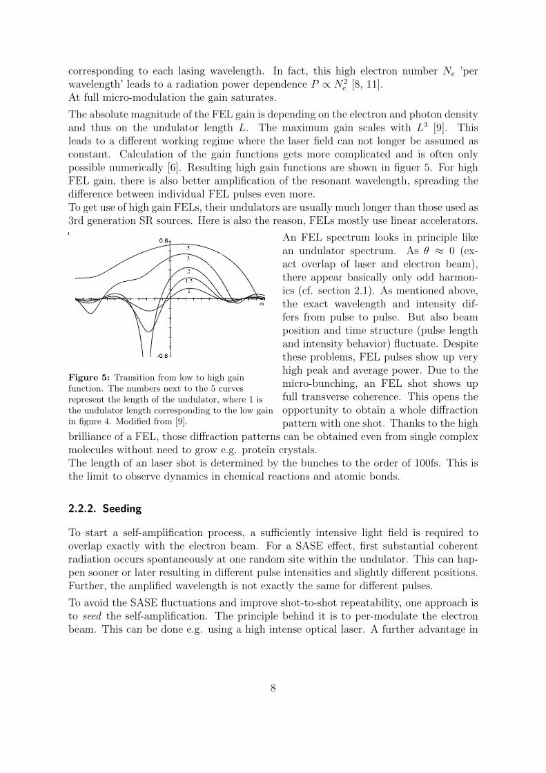
The absolute magnitude of the FEL gain is depending on the electron and photon densityand thus on the undulator length L. The maximum gain scales with L3 [9]. Thisleads to a different working regime where the laser field can not longer be assumed asconstant. Calculation of the gain functions gets more complicated and is often onlypossible numerically [6]. Resulting high gain functions are shown in figuer 5. For highFEL gain, there is also better amplification of the resonant wavelength, spreading thedifference between individual FEL pulses even more.To get use of high gain FELs, their undulators are usually much longer than those used as3rd generation SR sources. Here is also the reason, FELs mostly use linear accelerators.

Figure 5: Transition from low to high gainfunction. The numbers next to the 5 curvesrepresent the length of the undulator, where 1 isthe undulator length corresponding to the low gainin figure 4. Modified from [9].

An FEL spectrum looks in principle likean undulator spectrum. As θ ≈ 0 (ex-act overlap of laser and electron beam),there appear basically only odd harmon-ics (cf. section 2.1). As mentioned above,the exact wavelength and intensity dif-fers from pulse to pulse. But also beamposition and time structure (pulse lengthand intensity behavior) fluctuate. Despitethese problems, FEL pulses show up veryhigh peak and average power. Due to themicro-bunching, an FEL shot shows upfull transverse coherence. This opens theopportunity to obtain a whole diffractionpattern with one shot. Thanks to the high

brilliance of a FEL, those diffraction patterns can be obtained even from single complexmolecules without need to grow e.g. protein crystals.The length of an laser shot is determined by the bunches to the order of 100fs. This isthe limit to observe dynamics in chemical reactions and atomic bonds.

2.2.2. Seeding

To start a self-amplification process, a sufficiently intensive light field is required tooverlap exactly with the electron beam. For a SASE effect, first substantial coherentradiation occurs spontaneously at one random site within the undulator. This can hap-pen sooner or later resulting in different pulse intensities and slightly different positions.Further, the amplified wavelength is not exactly the same for different pulses.

To avoid the SASE fluctuations and improve shot-to-shot repeatability, one approach isto seed the self-amplification. The principle behind it is to per-modulate the electronbeam. This can be done e.g. using a high intense optical laser. A further advantage in

8

that case would be that the FEL is perfectly synchronized with an external optical laserfor pump-and-probe experiments [12].

However, it is a big effort to align the seeding laser sufficiently accurate to create condi-tions for self-amplification. The phase of the seeding light must match exactly with theundulator structure and its resulting electron bunch movement.

2.3. X-Ray Optics

Caused by the short wavelength and refraction indices n≈1, optics for x-rays must usedifferent principles than usual optics. To reflect x-rays, one can use either total externalreflection or Bragg diffraction. The first one is a result of shallow incidence angles onmaterials where n<nvacuum =1, as it appears for x-rays. The latter principle is usedwith single crystals or multilayer mirrors. In the multilayer case, radiation is reflectedby alternating films of different refraction indices with thicknesses matching to the usedphoton wavelength.

Using these principles, one can build mirroring and focusing devices. They again revealopportunities for monochromatization of white beams.The simplest way to focus a beam is to use toroidally shaped mirror. However, thiscan lead to a so called astigmatism, meaning the focal plane in horizontal and verticaldirection are different. To solve this problem, so called Kirkpatrick-Baez optics uses aset of two adjustable mirrors where each of them independently focuses the beam in onedirection.Another way of focusing uses a hastate tube. Pointing to a focus spot, x-rays are reflectedunder shallow angles on its inner surface.A different approach are Fresnel zone plates which use interference for focusing. Theycan be applied in reflection or transmission.Refractive lenses are difficult to realize because the refractive indices for x-rays are toonear at 1 for nearly all materials. Thus, rows of many concave lenses are needed.

It is important to mention that SR optics devices generally need to be cooled. This isdue to the heat load from penetration of the intense radiation into the material. Thisapplies especially for slits which are introduced to cut the beam size in order to get awell defined beam shape. Materials used for slits should also have high absorption (e.g.tungsten).

3. Setup at FLASH

FLASH is an around 300m long FEL in Hamburg. It produces pulses in the EUV and softx-ray regime. Pulse lengths down to 10fs have been achieved [1]. FLASH was upgradedseveral times and the construction of an extension called FLASH II is in progress.

9

315 m500 MeV 1.2 GeV150 MeV5 MeV

Laser

RF Gun

Diagnos-tics Accelerating Structures

Bunch Compressor

Bunch Compressor Collimator

Undulators

BypassFEL

Experiments

sFLASH

3rd harmonic

RF Stations

Figure 6: Longitudinal structure os FLASH [1].

3.1. Overview about FLASH

FLASH consists mainly of an electron source, linear accelerator and an long undulator.Figure 6 gives an overview about the flash setup.The electron source consists of a Cs2Te photocathode where electron bunches are injectedby an UV laser. The electrons are then accelerated by radio-frequent fields. This is whythe electron source is called RF gun. The charge of one bunch is 0.5 and 1 nC [1].A linear accelerator follows directly. Six modules of superconducting Nb-cavities raisethe electron energies up to 1.25GeV. This is done by high-voltage radio-freqnencies.The accelerator modules are interrupted by so called bunch compressors: During theacceleration in the cavities, the bunch velocity is determined by the radio frequency butthe energy gain is different for electrons at different longitudinal positions within thebunch. This makes, leading electrons in a bunch possess smaller energies than trailingones. Bunch compressors now are magnetic chicanes where the electrons are guided totravel a short distance with transverse offset. Thus the leading, smaller energy electronsare deflected stronger, travel a longer way and the bunch is compressed [1]. High electrondensities and short pulses become possible.Finally, the FEL beam is produced in a 27m long undulator line. Afterwards, the electronbeam is guided to a dump.Typical running parameters are listed in table 1.

Table 1: Typical operation parameters during the 2nd user period from Nov 26, 2007 to Aug 16,2009 [12].

parameter value

wavelength (fundamental) 6.8 - 47 nmaverage single pulse energy 10 - 100 µJpulse duration (FWHM) 10 - 70 fspeak power (from average) 1 - 5 GWaverage power for 500 pulses/sec ≈ 15 mWspectral bandwidth (FWHM) ≈ 1 %

peak brilliance 1029 - 1030 photonss mrad2mm20.1%bw

The undulators of FLASH have a fixed gap of 12mm. A change of the photon energy is

10

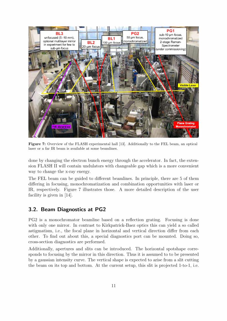
Figure 7: Overview of the FLASH experimental hall [13]. Additionally to the FEL beam, an opticallaser or a far IR beam is available at some beamlines.

done by changing the electron bunch energy through the accelerator. In fact, the exten-sion FLASH II will contain undulators with changeable gap which is a more convenientway to change the x-ray energy.

The FEL beam can be guided to different beamlines. In principle, there are 5 of themdiffering in focusing, monochromatization and combination opportunities with laser orIR, respectively. Figure 7 illustrates those. A more detailed description of the userfacility is given in [14].

3.2. Beam Diagnostics at PG2

PG2 is a monochromator beamline based on a reflection grating. Focusing is donewith only one mirror. In contrast to Kirkpatrick-Baez optics this can yield a so calledastigmatism, i.e., the focal plane in horizontal and vertical direction differ from eachother. To find out about this, a special diagnostics port can be mounted. Doing so,cross-section diagnostics are performed.

Additionally, apertures and slits can be introduced. The horizontal spotshape corre-sponds to focusing by the mirror in this direction. Thus it is assumed to to be presentedby a gaussian intensity curve. The vertical shape is expected to arise from a slit cuttingthe beam on its top and bottom. At the current setup, this slit is projected 1-to-1, i.e.

11

the spotsize should be equal to the length of the slit. This setup principles are shown infigure 8.

Further information about the PG2 beamline can be found in [15].

Figure 8: Sketch of the focusingprinciples at the PG2 setup. Greenrepresents the Ce:YAG crystal,black the mirror and exit slit.

3.2.1. Methods of Beam Diagnostics

Beam spot diagnostics can investigate spectral content,intensities, time structure or lateral information such asbeam spot positions and cross-sections. Spectral andintensity diagnostics is done e.g. online using a gasmonitor detector. This is important to get exact in-formation for each pulse independently. In this project,cross-section and lateral position diagnostics is done di-rectly, i.e. invasive.

For continuous beams, scans over slits, wires or gridsare common for this purpose. However, for FEL pulses this is not applicable as everyshot is different from another one. Thus, mainly two other ways are common: One is ae.g. Ce:YAG crystal as fluorescent screen and recording of the beam spot replica by aCCD camera. In this case, the screen prevents saturation and damage of the CCD andfurthermore allows to increase the spatial resolution by optical lens systems. Anotherway to obtain a footprint of the FEL beam is to investigate ablation craters in PMMA.However, this is more wavelength-sensitive [8].

In both cases, the focused spotsize and transverse intensity distribution are observed.Furthermore, information about beam divergence can be obtained. For those kind ofbeam diagnostics, special attention has to be paid to the difference between several FELshots. Therefore, an averaging mode or shot-to-shot diagnostics are applied. Whilethe first one tells about stability and main parameters of the FEL, the latter one isalso very important for experimental interpretation. Especially the fluorescent crystalmethod is well suited to discover the so called pointing stability, i.e. the relation betweenlateral shot-to-shot positions. Achieving a high pointing stability is very important forexperimental alignment.

4. The MATLAB Program: beamspotdiagnostics

As summer student project, a program with graphical user interface (GUI) was writ-ten. It consists of the main program beamspotdiagnostics.m with GUI binary filebeamspotdiagnostics.fig1 as well as a sub-program which exists in two different ver-sions, beamspotevaluation1.m and beamspotevaluation2.m, respectively.

1The binary .fig file is not necessarily needed. There is another version of beamspotdiagnostics.mthat already contains the GUI appearance information.

12

The purpose of the program is to analyze camera images from beam replica on a fluo-rescent crystal. For that, an arbitrary number of images can be chosen and evaluated atone run. Figure 9 shows the GUI which was created with the MATLAB tool GUIDE.The upper part of the window is used to choose the files and region of interest. In themiddle, evaluation parameters and information for output data are set. Finally, in thelower part, evaluated data is plotted.

In the upper listbox on the left, files are chosen from the local directories. Each chosen fileappears in the listbox below where a file list is collected for an evaluation run. (Filenamescan be deleted from this list again using the ’delete’ button.) It is important, that allselected files are saved in the same folder. Whenever a file is chosen using double mouseclick or return key at any listbox, it is plotted at the same time on the right. To define aregion of interest (where the beam spot appears), the user must click on the image plot.Then a crop tool will appear allowing to define a rectangle within the image. Afterwards,this region is plotted separately below.

There are two pairs of radio buttons to select the mode of evaluation: First, it is possibleto define if the data from all chosen images shall be averaged before running the evalu-ation or if single images should be evaluated one by one. In the latter case the averagevalues of these single evaluations are also calculated and plotted afterwards. The secondselection is if one or two spots are assumed in horizontal direction. The reason for thisoption is that often a slightly mis-aligned FEL leads to two laterally separated spotsinstead of one as it should be the case.When the evaluation is run, for each image (or for the average of the chosen images,respectively) the sub-program beamspotevaluation1.m (one spot in horizontal direc-tion) or beamspotevaluation2.m (two spots) is executed. These programs integratethe intensities of the images within the chosen region of interest along horizontal andvertical directions. Then, for the horizontal intensity curve a gaussian function (or tworespectively) is fitted to obtain the full width at half maximum (FWHM) and absolutespotposition. For the vertical intensity distribution, the programs directly search forhalf maximum values (cf. figure 10).

When the evaluation is done the results for FWHM and spot position are plotted in thebottom area of the user window. As abscissa, the longitudinal screen position is taken.This longitudinal position of the crystal must be set in the respective textfield above.The scale of FWHM and position are plotted in µm, based on the conversion factors theuser sets in the respective textfields. Default values are 4.1595µm/pixel in horizontaland 5.8824µm/pixel in vertical direction (due to a 45◦ tilted crystal). For the FWHM,the meanvalues for the longitudinal positions are calculated and plotted as line, for thepositions, the meanvalues are subtracted from each data point in the plot.

There are several output files produced by the beam diagnostics program: The evaluateddata is saved in file ’separately filename’ or ’averaged filename’, respectively, dependingon the evaluation mode chosen. Here, filename is the string that has to be defined bythe user in the corresponding textfield. These files contain the following seven columns:

position [mm] fwhmx1 [px] fwhmx2 [px] positionx1 [px] positionx2 [px] fwhmy [px] positiony [px]

13

Figure 9: Screenshot of the graphical user interface.

14

x is ment to be horizontal, y vertical direction. If the ’one spot’-mode is chosen insteadof two spots the 3rd and 5th column are filled with ’-1’.A second output file with the name ’meanvalues filename’ is produced. It contains fourcolumns:

position [mm] fwhmx1 [µm] fwhmx2 [µm] fwhmy [µm]

Here, the average values from the first output file are saved. Note that the values havebeen converted to µm.If the ’average before evaluation’ mode is selected, the an average image is also saved.Its name is ’averaged filename.bmp’.

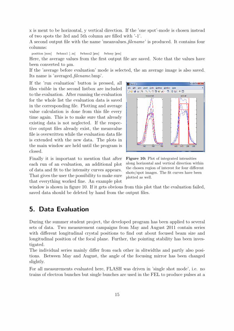
Figure 10: Plot of integrated intensitiesalong horizontal and vertical direction withinthe chosen region of interest for four differentshots/spot images. The fit curves have beenplotted as well.

If the ’run evaluation’ button is pressed, allfiles visible in the second listbox are includedto the evaluation. After running the evaluationfor the whole list the evaluation data is savedin the corresponding file. Plotting and averagevalue calculation is done from this file everytime again. This is to make sure that alreadyexisting data is not neglected. If the respec-tive output files already exist, the meanvaluefile is overwritten while the evaluation data fileis extended with the new data. The plots inthe main window are held until the program isclosed.

Finally it is important to mention that aftereach run of an evaluation, an additional plotof data and fit to the intensity curves appears.That gives the user the possibility to make surethat everything worked fine. An example plotwindow is shown in figure 10. If it gets obvious from this plot that the evaluation failed,saved data should be deleted by hand from the output files.

5. Data Evaluation

During the summer student project, the developed program has been applied to severalsets of data. Two measurement campaigns from May and August 2011 contain serieswith different longitudinal crystal positions to find out about focused beam size andlongitudinal position of the focal plane. Further, the pointing stability has been inves-tigated.The individual series mainly differ from each other in slitwidths and partly also posi-tions. Between May and August, the angle of the focusing mirror has been changedslightly.

For all measurements evaluated here, FLASH was driven in ’single shot mode’, i.e. notrains of electron bunches but single bunches are used in the FEL to produce pulses at a

15

rate of e.g. 10Hz. As described above, the FEL beam is treated with a monochromator atthe PG2 beamline. The single pulse energy was in the order of 5µJ for all measurements.However, the dependence of the beam properties on the pulse energy is not examinedhere.

For the pixel-to-µm conversion factors for the camera/lens system, 4.1595µm/pixel inhorizontal and 5.8824µm/pixel in vertical direction have been used. Errors are in theorder of 1 pixel.For the longitudinal position, ’-’ means closer to the mirror while ’+’ is further awayfrom it.

5.1. Data from May 2011

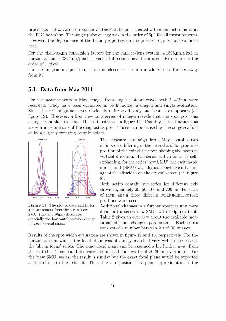
For the measurements in May, images from single shots at wavelength λ =19nm wererecorded. They have been evaluated in both modes, averaged and single evaluation.Since the FEL alignment was obviously quite good, only one beam spot appears (cf.figure 19). However, a first view on a series of images reveals that the spot positionschange from shot to shot. This is illustrated in figure 11. Possibly, these fluctuationsarose from vibrations of the diagnostics port. Those can be caused by the stage scaffoldor by a slightly swinging sample holder.

440 450 460 470

horizontal

440 460 480

vertical

Figure 11: The plot of data and fit fora measurement from the series ’newSMU’ (exit slit 50µm) illustratesespecially the horizontal position changebetween several shots.

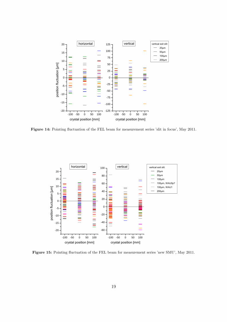
The measure campaign from May contains twomain series differing in the lateral and longitudinalposition of the exit slit system shaping the beam invertical direction. The series ’slit in focus’ is self-explaining, for the series ’new SMU’, the switchablemirror unit (SMU) was aligned to achieve a 1:1 im-age of the slitwidth on the crystal screen (cf. figure8).Both series contain sub-series for different exitslitwidth, namely 20, 50, 100 and 200µm. For eachof them again three different longitudinal screenpositions were used.Additional changes in a further aperture unit weredone for the series ’new SMU’ with 100µm exit slit.Table 2 gives an overview about the available mea-surements and changed parameters. Each seriesconsists of a number between 9 and 30 images.

Results of the spot width evaluation are shown in figure 12 and 13, respectively. For thehorizontal spot width, the focal plane was obviously matched very well in the case ofthe ’slit in focus’ series. The exact focal plane can be assumed a bit further away fromthe exit slit. That could decrease the focused spot width of 20-30µm even more. Forthe ’new SMU’ series, the result is similar but the exact focal plane would be expecteda little closer to the exit slit. Thus, the zero position is a good approximation of the

16

Table 2: Parameters for the different measurement series from May 2011.

exit slitposition exit slitwidth aperture unit screen position

in focus

20µm - -100, 0, 100mm50µm - -100, 0, 100mm100µm - -100, 0, 100mm200µm - -100, 0, 100mm

new SMU

20µm - -100, 0, 100mm50µm - -100, 0, 100mm100µm - -100, 0, 100mm100µm WAU 1 -100, 0, 100mm100µm WAU 0.7 -100, 0, 100mm200µm - -100, 0, 100mm

exact focal plane. As expected, the vertical exit slit does not influence the horizontalspot width.

In vertical direction, the dependence of the spot width on the slitwidth is clearly visible.However, the exact behaviour is far away from 1:1 imaging of the slitwidth. At zeroscreen position, the behaviour of the meanvalue for the single spot width can roughlybe described as spotwidth = 0.65*slitwidth + 100µm.The dependence on the screen position seems to be widely dominated by fluctuationseven if minima appear around the zero position. It is not clear why the series for 100µmexit slit shows a different behavior regarding to the vertical spot width. One reason canbe a lateral mis-alignment of the slit system. That could also explain the difference ofthe curve slopes, i.e. for 20 and 50µm the smallest vertical spot width tends to appearat slightly positive screen positions (further away from the exit slit) while for 100 and200µm it behaves vice versa.

Comparing the results from the evaluation of averaged data and the averages of singleshot evaluations, the averages FWHM tend to be 10-40µm larger in vertical and in theorder of 5µm larger in horizontal direction. This was expected due to spot positionfluctuations (cf, figure 11). The shot-to-shot fluctuation broadens the spot more than15% in vertical and more than 10% in horizontal direction.

For the series ’new SMU’, there is also a dependence of the spot width on the change of awater-cooled aperture unit (WAU): While the vertical FWHM curves are similar for allWAU settings, the horizontal spot width is dramatically changed from approximately 40to 30 to 20 µm (at zero screen position) from WAU 0.7 to WAU 1 to the usual setting.Thus, the setting without aperture changes can be assumed to correspond to WAU xwith x>1.

A closer look on the pointing stability (single shot evaluation) is done in the plots 14and 15. The horizontal position fluctuations from one shot to another are spread upto ±15µm (at zero crystal position). That corresponds to about 50% of the spotwidthand verifies once again that the main reason for the difference between single spot and

17

- 1 0 0 - 5 0 0 5 0 1 0 0

7 5

1 0 0

1 2 5

1 5 0

1 7 5

2 0 0

2 2 5

2 5 0

2 7 5

3 0 0

3 2 5

3 5 0 ������ ����

� ��� ����������������������������������������������� ��� ��������

������ ���������������!����!�����!�����!�

����

����

����� ���������������- 1 0 0 - 5 0 0 5 0 1 0 0

1 5

2 0

2 5

3 0

3 5

4 0

4 5���� ��� ����

����� ���������������

Figure 12: Lateral width of the focused beam on the fluorescent crystal. Measurement series ’slit infocus’, May 2011.

- 1 0 0 - 5 0 0 5 0 1 0 0

1 0 0

1 5 0

2 0 0

2 5 0

3 0 0!�� ��������

����

����

��#� ������� ��������

��!����������������������� ������������������� ����������!����������

!�� ������"� ���� ����%����%�����%�����%���� �������%���� �����%�

- 1 0 0 - 5 0 0 5 0 1 0 01 5

2 0

2 5

3 0

3 5

4 0

4 5

5 0

5 5����$�� ������

��#� ������� ��������

Figure 13: Lateral width of the focused beam on the fluorescent crystal. Measurement series ’newSMU’, May 2011.

18

- 1 0 0 - 5 0 0 5 0 1 0 0- 2 0

- 1 5

- 1 0

- 5

0

5

1 0

1 5

2 0

- 1 0 0 - 5 0 0 5 0 1 0 0- 1 2 5- 1 0 0- 7 5- 5 0- 2 5

02 55 07 5

1 0 01 2 5 ���� � ���� ���� ���� ��

����������������������

�� ���

�����

������

����

�

��������� � �������

��� �����

��������� � �������

Figure 14: Pointing fluctuation of the FEL beam for measurement series ’slit in focus’, May 2011.

- 1 0 0 - 5 0 0 5 0 1 0 0

- 2 0

- 1 5

- 1 0

- 5

0

5

1 0

1 5

2 0����������

�� ���

�����

������

����

�

��������������������

���������������������������������������������������������������

- 1 0 0 - 5 0 0 5 0 1 0 0

- 6 0

- 4 0

- 2 0

0

2 0

4 0

6 0

8 0

1 0 0 ��������

��������������������

Figure 15: Pointing fluctuation of the FEL beam for measurement series ’new SMU’, May 2011.

19

average evaluation is a bad pointing stability. The horizontal pointing stability is inde-pendent on the vertical exit slit.The vertical pointing fluctuation can reach more than ±50µm (again at zero crystal posi-tion). It scales with the exit slit roughly like fluctuation = ± 0.5*(0.45*slitwidth+30µm).The additional aperture does not affect the pointing stability. Position fluctuations in-crease also if the focal plane is not matched by the longitudinal crystal position.

5.2. Data from August 2011

For the measurements from August, the angle of the focusing mirror was changed by1mrad. A wavelength of λ =6.3nm was used. The diagnostics port scaffold was mademore stable in order to avoid vibrational influences. However, two different problemsarose: First, due to a slightly mis-aligned FEL, two laterally separated beam spotsappear and show up strong intensity fluctuations from shot to shot. Second, all imagesare the sum of two shots as the camera took data with 5Hz rate, while the FEL workedat 10Hz pulse rate.

Again, measurements with different longitudinal crystal positions were performed fordifferent slitwidths. There are two main series differing in the longitudinal position ofthe exit slit. The effect on the vertical spotsize can be investigated. An overview aboutthe measurements series is given in table 3. Each series consists of at least 20, maximum60 images.

Table 3: Parameters for the different measurement series from August 2011.

longitud. exit slitpos. exit slitwidth screen position

14020µm -100, -50, 0, 50, 100mm50µm -100, -50, 0, 50, 100mm100µm -100, -50, 0, 50, 100mm

18020µm -100, -50, 0, 50, 100mm50µm -100, -50, 0, 50, 100mm100µm -100, -50, 0, 50, 100mm

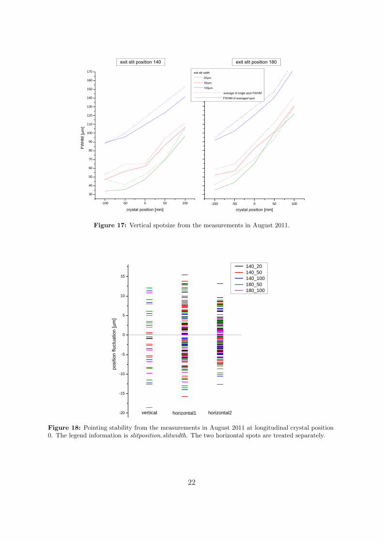
The plots in figures 16 and 17 contain the spot widths (FWHM) in horizontal and verticaldirection for both exit slit positions. Again, the horizontal focus plane is matched quitewell. At the same time strong fluctuations affect the curves. Those result from the twooverlapping beam spots. Two spots can arise e.g. from wrong time structure due to notexact RF phase during electron bunch acceleration in the FEL. Such a disturbed bunchstructure can be transferred into a changed lateral structure in the unduluator. Thefluctuations have even more effect than the difference between single shot evaluationand averaged one.In vertical direction, the focal plane is obviously closer to the exit slit. This is expectedsince a 1:1 imaging of the exit slitwidth on the crystal was wanted for zero screenposition (cf. figure 8) and repesents the astigmastism of the system. However, the

20

- 1 0 0 - 5 0 0 5 0 1 0 02 0

3 0

4 0

5 0

6 0

7 0

8 0

9 0

1 0 0

1 1 0

1 2 0

��!�����������������

����

����

��!����������������� - 1 0 0 - 5 0 0 5 0 1 0 0

� ��������������������� �������������

���"����"�����"�

����������������������������������������������

� ��������������������

Figure 16: Horizontal spotsize from the measurements in August 2011. For each condition two spotsappear - a smaller and a larger one.

vertical spotwidth is larger than the exitslit width. The spotwidth follows approximately0.75*slitwidth + 30µm for slitposition 140 and 0.60*slitwidth + 50µm for slitposition 180.The horizontal spotwidth is also slightly affected, probably due to unexact alignment.The two beam spots have horizontal width of about 30 and 50µm, respectively.

Even if the appearance of two laterally separated beam spots cause strong fluctuations inthe corresponding spotwidths there is less vertical spotposition fluctuation in the Augustdata than in May. Figure 18 confirms that vertical and horizontal pointing stability arein the same range of about ±15µm. Reasons for the vertical improvement can be thenew additional stabilization of the diagnostics port or better exitslit alignment.

Nevertheless, there is a further noteable fact about the intensity curves (cf. figures 10and 11): Regarding to the machine setup we assume a gaussian shape in horizontaldirection and a constant intensity vertically. However, the vertical intensity curve doesnot show a flat plateau (top of a broadened gaussian) with sharp edges from the exitslit.Instead, several maxima on changing positions appear. This is probably because offluctuations, spatial irregularities or a slight misalignment.

21

- 1 0 0 - 5 0 0 5 0 1 0 0

3 0

4 0

5 0

6 0

7 0

8 0

9 0

1 0 0

1 1 0

1 2 0

1 3 0

1 4 0

1 5 0

1 6 0

1 7 0

��!�����������������

����

����

��!����������������� - 1 0 0 - 5 0 0 5 0 1 0 0

� ��������������������� �������������

���"����"�����"�� ��������������������������

���������������������

� ��������������������

Figure 17: Vertical spotsize from the measurements in August 2011.

- 2 0

- 1 5

- 1 0

- 5

0

5

1 0

1 5 1 4 0 _ 2 0 1 4 0 _ 5 0 1 4 0 _ 1 0 0 1 8 0 _ 5 0 1 8 0 _ 1 0 0

h o r i z o n t a l 2

�� ���

�����

������

����

�

v e r t i c a l h o r i z o n t a l 1

Figure 18: Pointing stability from the measurements in August 2011 at longitudinal crystal position0. The legend information is slitposition slitwidth. The two horizontal spots are treated separately.

22

5.3. Conclusion

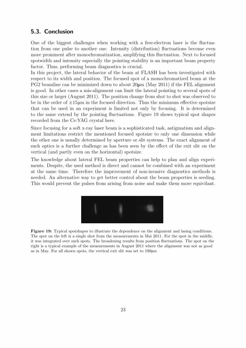
One of the biggest challenges when working with a free-electron laser is the fluctua-tion from one pulse to another one. Intensity (distribution) fluctuations become evenmore prominent after monochromatization, amplifying this fluctuation. Next to focusedspotwidth and intensity especially the pointing stability is an important beam propertyfactor. Thus, performing beam diagnostics is crucial.In this project, the lateral behavior of the beam at FLASH has been investigated withrespect to its width and position. The focused spot of a monochromatized beam at thePG2 beamline can be minimized down to about 20µm (May 2011) if the FEL alignmentis good. In other cases a mis-alignment can limit the lateral pointing to several spots ofthis size or larger (August 2011). The position change from shot to shot was observed tobe in the order of ±15µm in the focused direction. Thus the minimum effective spotsizethat can be used in an experiment is limited not only by focusing. It is determinedto the same extend by the pointing fluctuations. Figure 19 shows typical spot shapesrecorded from the Ce:YAG crystal here.

Since focusing for a soft x-ray laser beam is a sophisticated task, astigmatism and align-ment limitations restrict the mentioned focused spotsize to only one dimension whilethe other one is usually determined by aperture or slit systems. The exact alignment ofsuch optics is a further challenge as has been seen by the effect of the exit slit on thevertical (and partly even on the horizontal) spotsize.

The knowledge about lateral FEL beam properties can help to plan and align experi-ments. Despite, the used method is direct and cannot be combined with an experimentat the same time. Therefore the improvement of non-invasive diagnostics methods isneeded. An alternative way to get better control about the beam properties is seeding.This would prevent the pulses from arising from noise and make them more equivilant.

Figure 19: Typical spotshapes to illustrate the dependence on the alignment and lasing conditions.The spot on the left is a single shot from the measurements in Mai 2011. For the spot in the middle,it was integrated over such spots. The broadening results from position fluctuations. The spot on theright is a typical example of the measurements in August 2011 where the alignment was not as goodas in May. For all shown spots, the vertical exit slit was set to 100µm

23

APPENDIX

A. Source Code

The shown source code is only the part containing the most important functionality. Todetermine layout and graphics object handling there is a lot more code.

A.1. Extract of GUI beamspotdiagnostics.m

1 function varargout = GUI beamspotdiagnost ics ( vararg in )

9 % This GUI he l p s to e va l ua t e a s e t o f beamspot images ( e . g . from a10 % f l ou r en s c en t c r y s t a l ) wi th r e s p e c t to the spo t s i z e s and p o s i t i o n s in11 % ho r i z on t a l and v e r t i c a l d i r e c t i o n . For eva lua t ion , i t can be chosen12 % between s i n g l e e va l ua t i on f o r each image or averag ing over a l l chosen13 % images b e f o r e e va l ua t i on . Furthermore i t can be chosen whether one or14 % two gauss ian spo t s occure in h o r i z on t a l d i r e c t i o n . I f two are s e l e c t e d ,15 % they are t r e a t e d s e p a r a t e l y .16 %17 % Resu l t s are saved in t o an ASCII f i l e con ta in ing 7 colums :18 % 1: l a t e r a l p o s i t i o n o f the screen [mm] ( to be typed in at the GUI)19 % 2: width o f the f i r s t gauss ian in x−dimension [ px ]20 % 3: width o f the second gauss ian in x−dimension [ px ] ( on ly i f 2 spo t s )21 % 4: a b s o l u t e p o s i t i o n o f the f i r s t maximum in x−dimension [ px ]22 % 5: a b s o l u t e p o s i t i o n o f the second maximum in x−dimension [ px ] ( on ly23 % i f 2 spo t s )24 % 6: width in y−dimension [ px ]25 % 7: po s i t i o n in y−dimension [ px ]26 % Depending on the chosen e va l ua t i on mode , the name o f t h i s f i l e i s e i t h e r27 % ’ averaged typed f i l ename ’ or ’ s e pa ra t e l y t y p ed f i l e name ’ . I f the f i l e28 % already e x i s t s , data i s appended .29 %30 % Average va l u e s are saved in an add i t i o n a l a s c i i f i l e con ta in ing 4 colums

:31 % 1: l a t e r a l p o s i t i o n o f the screen [mm] ( to be typed in at the GUI)32 % 2: average width o f the f i r s t gauss ian in x−dimension [ m ]33 % 3: average width o f the second gauss ian in x−dimension [ m ] ( on ly i f 2

spo t s )34 % 4: average width in y−dimension [ m ]35 % The name o f t h i s f i l e i s ’ meanva lues typedf i l ename ’ . I t i s o v e rwr i t t en

i f36 % already e x i s t i n g .

99 % Globa l v a r i a b l e s100 handles . r o i c o o r d i n a t e s =[1 1 1 1 ] ;101 handles . imagebuf f e r = [ ] ;

137 % CALLBACK FUNCTIONS TO GUI ELEMENTS:138

139 % −−− Executes on s e l e c t i o n change in l i s t b o x 1 .

24

140 function l i s t b o x 1 C a l l b a c k ( hObject , eventdata , handles ) % l i s t o f curren tf o l d e r content

141 % hObject handle to l i s t b o x 1 ( see GCBO)142 % eventda ta re se rved − to be de f ined in a f u t u r e ve r s i on o f MATLAB143 % hand les s t r u c t u r e wi th hand les and user data ( see GUIDATA)144

145 set ( handles . l i s tbox1 , ’ HitTest ’ , ’ o f f ’ ) ;146 i f strcmp (get ( handles . f i gu r e1 , ’ Se lect ionType ’ ) , ’ open ’ )147 f i l e l i s t = get ( handles . l i s tbox1 , ’ S t r ing ’ ) ;148 i n d e x s e l e c t e d = get ( handles . l i s tbox1 , ’ Value ’ ) ;149 f i l ename = f i l e l i s t { i n d e x s e l e c t e d } ;150 i f handles . i s d i r ( handles . s o r t e d i nd e x ( i n d e x s e l e c t e d ) )151 cd ( f i l ename )152 l o a d l i s t b o x (pwd, handles )153 else154 [path , name , ext ] = f i l e p a r t s ( f i l ename ) ;155 i f strcmp ( ext , ’ .bmp ’ )156 t ry157 e n t r i e s = get ( handles . l i s tbox2 , ’ S t r ing ’ ) ;158 e n t r i e s {end+1}=f i l ename ;159 e n t r i e s=sort ( e n t r i e s ) ;160 set ( handles . l i s tbox2 , ’ S t r ing ’ , e n t r i e s ) ;161 handles . imagebuf f e r=imread ( f i l ename ) ;162 guidata ( hObject , handles ) ;163 set ( handles . f i gu r e1 , ’ CurrentAxes ’ , handles . axes2 ) ;164 image( handles . imagebuf fer , ’ HitTest ’ , ’ o f f ’ ) ;165 set ( handles . axes2 , ’ ButtonDownFcn ’ , {@axes2 ButtonDownFcn ,

handles }) ;166 catch ex167 e r r o r d l g ( . . .168 ex . getReport ( ’ ba s i c ’ ) , ’ F i l e Type Error ’ , ’ modal ’ )169 end170 end171 end172 end173 set ( handles . l i s tbox1 , ’ HitTest ’ , ’ on ’ ) ;174

175 % −−− Executes on key pre s s wi th focus on l i s t b o x 1 and none o f i t sc on t r o l s .

176 function l i s tbox1 KeyPressFcn ( hObject , eventdata , handles ) % l i s t o fcurren t f o l d e r content

177 % hObject handle to l i s t b o x 1 ( see GCBO)178 % eventda ta s t r u c t u r e wi th the f o l l ow i n g f i e l d s ( see UICONTROL)179 % Key : name o f the key t ha t was pressed , in lower case180 % Character : charac t e r i n t e r p r e t a t i o n o f the key ( s ) t ha t was pres sed181 % Modi f ier : name( s ) o f the mod i f i e r key ( s ) ( i . e . , con t ro l , s h i f t )

pres sed182 % hand les s t r u c t u r e wi th hand les and user data ( see GUIDATA)183 i f strcmp ( eventdata . Key , ’ r e turn ’ ) & get ( handles . l i s tbox1 , ’ Value ’ )184 set ( handles . l i s tbox1 , ’ HitTest ’ , ’ o f f ’ ) ;185 f i l e l i s t = get ( handles . l i s tbox1 , ’ S t r ing ’ ) ;186 i n d e x s e l e c t e d = get ( handles . l i s tbox1 , ’ Value ’ ) ;

25

187 d i r e c t o r i e s =0;%check i f on ly f i l e s s e l e c t e d188 for a=1: length ( i n d e x s e l e c t e d )189 i f i s d i r ( f i l e l i s t { i n d e x s e l e c t e d ( a ) })190 d i r e c t o r i e s =1;191 end192 end193 i f d i r e c t o r i e s==0194 for a=2: length ( i n d e x s e l e c t e d )195 f i l ename = f i l e l i s t { i n d e x s e l e c t e d ( a ) } ;196 [path , name , ext ] = f i l e p a r t s ( f i l ename ) ;197 i f strcmp ( ext , ’ .bmp ’ )198 t ry199 e n t r i e s = get ( handles . l i s tbox2 , ’ S t r ing ’ ) ;200 e n t r i e s {end+1}=f i l ename ;201 set ( handles . l i s tbox2 , ’ S t r ing ’ , e n t r i e s ) ;202 handles . imagebuf f e r=imread ( f i l ename ) ;203 guidata ( hObject , handles ) ;204 set ( handles . f i gu r e1 , ’ CurrentAxes ’ , handles . axes2 ) ;205 image( handles . imagebuf fer , ’ HitTest ’ , ’ o f f ’ ) ;206 set ( handles . axes2 , ’ ButtonDownFcn ’ , {@axes2 ButtonDownFcn ,

handles }) ;207 catch ex208 e r r o r d l g ( . . .209 ex . getReport ( ’ ba s i c ’ ) , ’ F i l e Type Error ’ , ’ modal ’ )210 end211 end212 end213 end214 set ( handles . l i s tbox1 , ’ HitTest ’ , ’ on ’ ) ;215 end216

217

218 % −−− Executes on s e l e c t i o n change in l i s t b o x 2 .219 function l i s t b o x 2 C a l l b a c k ( hObject , eventdata , handles ) % l i s t o f chosen

f i l e s220 % hObject handle to l i s t b o x 2 ( see GCBO)221 % eventda ta re se rved − to be de f ined in a f u t u r e ve r s i on o f MATLAB222 % hand les s t r u c t u r e wi th hand les and user data ( see GUIDATA)223

224 get ( handles . f i gu r e1 , ’ Se lect ionType ’ ) ;225 i f strcmp (get ( handles . f i gu r e1 , ’ Se lect ionType ’ ) , ’ open ’ )226 i n d e x s e l e c t e d = get ( handles . l i s tbox2 , ’ Value ’ ) ;227 f i l e l i s t = get ( handles . l i s tbox2 , ’ S t r ing ’ ) ;228 f i l ename = f i l e l i s t { i n d e x s e l e c t e d } ;229 [path , name , ext ] = f i l e p a r t s ( f i l ename ) ;230 i f strcmp ( ext , ’ .bmp ’ )231 t ry232 handles . imagebuf f e r=imread ( f i l ename ) ;233 guidata ( hObject , handles ) ;234 set ( handles . f i gu r e1 , ’ CurrentAxes ’ , handles . axes2 ) ;235 image( handles . imagebuf fer , ’ HitTest ’ , ’ o f f ’ ) ;

26

236 set ( handles . axes2 , ’ ButtonDownFcn ’ , {@axes2 ButtonDownFcn ,handles }) ;

237 catch ex238 e r r o r d l g ( . . .239 ex . getReport ( ’ ba s i c ’ ) , ’ F i l e Type Error ’ , ’ modal ’ )240 end241 end242 end243

244 % −−− Executes on key pre s s wi th focus on l i s t b o x 2 and none o f i t sc on t r o l s .

245 function l i s tbox2 KeyPressFcn ( hObject , eventdata , handles ) % l i s t o fchosen f i l e s

246 % hObject handle to l i s t b o x 2 ( see GCBO)247 % eventda ta s t r u c t u r e wi th the f o l l ow i n g f i e l d s ( see UICONTROL)248 % Key : name o f the key t ha t was pressed , in lower case249 % Character : charac t e r i n t e r p r e t a t i o n o f the key ( s ) t ha t was pres sed250 % Modi f ier : name( s ) o f the mod i f i e r key ( s ) ( i . e . , con t ro l , s h i f t )

pres sed251 % hand les s t r u c t u r e wi th hand les and user data ( see GUIDATA)252 i f strcmp ( eventdata . Key , ’ d e l e t e ’ ) & get ( handles . l i s tbox2 , ’ Value ’ )253 f i l e l i s t = get ( handles . l i s tbox2 , ’ S t r ing ’ ) ;254 i n d e x s e l e c t e d = get ( handles . l i s tbox2 , ’ Value ’ ) ;255 f i l e l i s t ( i n d e x s e l e c t e d ) = [ ] ;256 set ( handles . l i s tbox2 , ’ S t r ing ’ , f i l e l i s t ) ;257 set ( handles . l i s tbox2 , ’ Value ’ , 1 ) ;258 guidata ( hObject , handles ) ;259

260 end

296 % −−− Executes on but ton pre s s in pushbut ton2 .297 function pushbutton2 Cal lback ( hObject , eventdata , handles ) % Button to

s t a r t e va l ua t i on298 % hObject handle to pushbut ton2 ( see GCBO)299 % eventda ta re se rved − to be de f ined in a f u t u r e ve r s i on o f MATLAB300 % hand les s t r u c t u r e wi th hand les and user data ( see GUIDATA)301 hold on ;302 %eva l ua t i on and sav ing303 i f ˜strcmp (get ( handles . l i s tbox2 , ’ S t r ing ’ ) , ’ ’ )304 samples=get ( handles . l i s tbox2 , ’ S t r ing ’ ) ;305 f igure ;306 f i l ename=’ ’ ;307 switch get ( handles . radiobutton1 , ’ Value ’ )308 case 0309 f i l ename =[ ’ s e p a r a t e l y ’ , get ( handles . ed i t2 , ’ S t r ing ’ ) ] ;310 i f ˜exist ( f i l ename , ’ f i l e ’ )311 f i d = fopen ( f i l ename , ’wt ’ ) ;312 fpr intf ( f i d , ’%s %s %s %s %s %s %s ’ , [ ’ p o s i t i o n [mm] ’ ’

fwhmx1 [ px ] ’ ’ fwhmx2 [ px ] ’ ’ po s i t i o nx1 [ px ] ’ ’po s i t i o nx2 [ px ] ’ ’ fwhmy [ px ] ’ ’ p o s i t i o n y [ px ] ’ ] );

313 fpr intf ( f i d , ’ \n ’ ) ;314 fc lose ( f i d ) ;

27

315 end316 switch get ( handles . radiobutton3 , ’ Value ’ )317 case 1318 for a=1: length ( samples )319 oneeva luat ion=spoteva lua t i on1 ({ samples {a } , round(

handles . r o i c o o r d i n a t e s (1 ) ) , round( handles .r o i c o o r d i n a t e s (2 ) ) , round( handles . r o i c o o r d i n a t e s (3 )) , round( handles . r o i c o o r d i n a t e s (4 ) ) }) ; % { i n p u t f i l e, x s t a r t , y s t a r t , xwidth , ywidth }

320 oneeva luat ion =[str2num(get ( handles . ed i t1 , ’ S t r ing ’ ) ) ,oneeva luat ion ] ;

321 save ( f i l ename , ’ oneeva luat ion ’ , ’−a s c i i ’ , ’−append ’ ) ;322 end323 case 0324 for a=1: length ( samples )325 oneeva luat ion=spoteva lua t i on2 ({ samples {a } , round(

handles . r o i c o o r d i n a t e s (1 ) ) , round( handles .r o i c o o r d i n a t e s (2 ) ) , round( handles . r o i c o o r d i n a t e s (3 )) , round( handles . r o i c o o r d i n a t e s (4 ) ) }) ; % { i n p u t f i l e, x s t a r t , y s t a r t , xwidth , ywidth }

326 oneeva luat ion =[str2num(get ( handles . ed i t1 , ’ S t r ing ’ ) ) ,oneeva luat ion ] ;

327 save ( f i l ename , ’ oneeva luat ion ’ , ’−a s c i i ’ , ’−append ’ ) ;328 end329 end330 case 1331 f i l ename =[ ’ averaged ’ , get ( handles . ed i t2 , ’ S t r ing ’ ) ] ;332 i f ˜exist ( f i l ename , ’ f i l e ’ )333 f i d = fopen ( f i l ename , ’wt ’ ) ;334 fpr intf ( f i d , ’%s %s %s %s %s %s %s ’ , [ ’ p o s i t i o n [mm] ’ ’

fwhmx1 [ px ] ’ ’ fwhmx2 [ px ] ’ ’ po s i t i o nx1 [ px ] ’ ’po s i t i o nx2 [ px ] ’ ’ fwhmy [ px ] ’ ’ p o s i t i o n y [ px ] ’ ] );

335 fpr intf ( f i d , ’ \n ’ ) ;336 fc lose ( f i d ) ;337 end338 sampleaverage=imread ( samples {1}) / length ( samples ) ;339 for a=2: length ( samples )340 sampleaverage=sampleaverage+imread ( samples {a }) / length (

samples ) ;341 end342 sampleaverage=sampleaverage ;343 imwrite ( sampleaverage , [ f i l ename , ’ .bmp ’ ] , ’bmp ’ )344 switch get ( handles . radiobutton3 , ’ Value ’ )345 case 1346 oneeva luat ion=spoteva lua t i on1 ( { [ f i l ename , ’ .bmp ’ ] , round

( handles . r o i c o o r d i n a t e s (1 ) ) , round( handles .r o i c o o r d i n a t e s (2 ) ) , round( handles . r o i c o o r d i n a t e s (3 ) ) ,round( handles . r o i c o o r d i n a t e s (4 ) ) }) ; % { i n p u t f i l e ,x s t a r t , y s t a r t , xwidth , ywidth }

347 case 0

28

348 oneeva luat ion=spoteva lua t i on2 ( { [ f i l ename , ’ .bmp ’ ] , round( handles . r o i c o o r d i n a t e s (1 ) ) , round( handles .r o i c o o r d i n a t e s (2 ) ) , round( handles . r o i c o o r d i n a t e s (3 ) ) ,round( handles . r o i c o o r d i n a t e s (4 ) ) }) ; % { i n p u t f i l e ,x s t a r t , y s t a r t , xwidth , ywidth }

349 end350 oneeva luat ion =[str2num(get ( handles . ed i t1 , ’ S t r ing ’ ) ) ,

oneeva luat ion ] ;351 save ( f i l ename , ’ oneeva luat ion ’ , ’−a s c i i ’ , ’−append ’ ) ;352 end353 end354 hold o f f ;355 %p l o t t i n g356 p l o t b u f f e r=p l o t p r ep a r a t i on ( handles ) ;357 r e s u l t d a t a=p l o t b u f f e r {1 ,1} ;358 averages=p l o t b u f f e r {1 ,2} ;359 set ( handles . f i gu r e1 , ’ CurrentAxes ’ , handles . axes4 ) ;360 hold on ;361 p1=plot ( r e s u l t d a t a ( : , 1 ) , r e s u l t d a t a ( : , 2 ) , ’ r+’ ) ; %fwhmx1362 plot ( averages ( : , 1 ) , averages ( : , 2 ) , ’ r−− ’ )% average fwhmx1363 i f ˜sum( r e s u l t d a t a (1 , 3 )<0)>0364 plot ( r e s u l t d a t a ( : , 1 ) , r e s u l t d a t a ( : , 3 ) , ’ r+’ ) %fwhmx2365 plot ( averages ( : , 1 ) , averages ( : , 3 ) , ’ r−− ’ )% average fwhmx2366 end367 p2=plot ( r e s u l t d a t a ( : , 1 ) , r e s u l t d a t a ( : , 6 ) , ’ g+’ ) ; %fwhmy368 plot ( averages ( : , 1 ) , averages ( : , 4 ) , ’ g−− ’ )% average fwhmy369 t i t l e ( ’FWHM vs . s c r e en p o s i t i o n ’ , ’ FontSize ’ ,12) ;370 xlabel ( ’mm’ ) ;371 ylabel ( ’ m ’ ) ;372 hold o f f ;373 set ( handles . f i gu r e1 , ’ CurrentAxes ’ , handles . axes5 ) ;374 hold on ;375 p3=plot ( r e s u l t d a t a ( : , 1 ) , r e s u l t d a t a ( : , 4 ) , ’ r+’ ) ; %po s i t i o n x1376 i f ˜sum( r e s u l t d a t a (1 , 3 )<0)>0377 p4=plot ( r e s u l t d a t a ( : , 1 ) , r e s u l t d a t a ( : , 5 ) , ’ r+’ ) ; %po s i t i o n x2378 end379 p5=plot ( r e s u l t d a t a ( : , 1 ) , r e s u l t d a t a ( : , 7 ) , ’ g+’ ) ; %po s i t i o n y380 legend ( [ p3 p5 ] ,{ ’ h o r i z o n t a l ’ ’ v e r t i c a l ’ } , ’ Locat ion ’ , ’ Best ’ ) ;381 t i t l e ( ’ spot p o s i t i o n f l u c t u a t i o n vs . s c r e en p o s i t i o n ’ , ’ FontSize ’ ,12) ;382 xlabel ( ’mm’ ) ;383 ylabel ( ’ m ’ ) ;384 hold o f f ;385 %save averages o f fwhm386 f i l ename =[ ’ meanvalues ’ , get ( handles . ed i t2 , ’ S t r ing ’ ) ] ;387 f i d = fopen ( f i l ename , ’wt ’ ) ;388 fpr intf ( f i d , ’%s %s %s %s ’ , [ ’ p o s i t i o n [mm] ’ ’ fwhmx1 [ m ] ’ ’

fwhmx2 [ m ] ’ ’ fwhmy [ m ] ’ ] ) ;389 fpr intf ( f i d , ’ \n ’ ) ;390 fc lose ( f i d ) ;391 save ( f i l ename , ’ averages ’ , ’−a s c i i ’ , ’−append ’ ) ;392

393

29

394 % −−− Executes on mouse pre s s over axes background .395 function axes2 ButtonDownFcn ( hObject , eventdata , handles ) % image p l o t396 % hObject handle to axes2 ( see GCBO)397 % eventda ta re se rved − to be de f ined in a f u t u r e ve r s i on o f MATLAB398 % hand les s t r u c t u r e wi th hand les and user data ( see GUIDATA399 set ( handles . f i gu r e1 , ’ CurrentObject ’ , handles . axes2 ) ;400 t ry401 [ r o i r e c t ] = imcrop ( handles . axes2 ) ;402 handles . r o i c o o r d i n a t e s=r e c t ;403 guidata ( hObject , handles ) ;404 set ( handles . f i gu r e1 , ’ CurrentAxes ’ , handles . axes3 ) ;405 set ( handles . axes3 , ’XLim ’ , [ 0 r e c t (3 ) ] , ’YLim ’ , [ 0 r e c t (4 ) ] ) ;406 image( r o i ) ;407 catch e r r408 disp ( ’ t ry again ’ )409 end

462 % FURTHER FUNCTIONS USED BY THE CALLBACKS :463

464 % func t i on to read the curren t d i r e c t o r y and so r t the names465 function l o a d l i s t b o x ( d i r path , handles )466 cd ( d i r pa th )467 d i r s t r u c t = dir ( d i r pa th ) ;468 [ sorted names , s o r t e d i nd e x ] = sor t rows ({ d i r s t r u c t . name} ’ ) ;469 handles . f i l e n a m e s = sorted names ;470 handles . i s d i r = [ d i r s t r u c t . i s d i r ] ;471 handles . s o r t e d i nd e x = s o r t e d i nd e x ;472 guidata ( handles . f i gu r e1 , handles ) ;473 set ( handles . l i s tbox1 , ’ S t r ing ’ , handles . f i l e names , . . .474 ’ Value ’ , 1 )475 set ( handles . text1 , ’ S t r ing ’ ,pwd)476

477

478 % prepar ing data from the t a r g e t f i l e f o r p l o t t i n g ( i n c l . averagec a l c u l a t i o n )

479 function p lotdata=p lo tp r e pa ra t i o n ( handles )480 switch get ( handles . radiobutton1 , ’ Value ’ )481 case 1482 f i l ename =[ ’ averaged ’ , get ( handles . ed i t2 , ’ S t r ing ’ ) ] ;483 case 0484 f i l ename =[ ’ s e p a r a t e l y ’ , get ( handles . ed i t2 , ’ S t r ing ’ ) ] ;485 end486 r e s u l t d a t a = g e t f i e l d ( importdata ( f i l ename ) , ’ data ’ ) ;487 f igure ( handles . f i g u r e 1 ) ;488 % average va lue c a l c u l a t i o n f o r p l o t489 r e s u l t d a t a=sort rows ( r e su l tda ta , 1 ) ;490 s c r e e n p o s i t i o n = [ ] ;491 averagesxw1 = [ ] ;492 averagesxp1 = [ ] ;493 averagesxw2 = [ ] ;494 averagesxp2 = [ ] ;495 averagesyp = [ ] ;496 averagesyw = [ ] ;

30

497 c2 =0;498 c4 =0;499 a=1;500 while a<=length ( r e s u l t d a t a ( : , 1 ) )501 counter =1;502 c1=r e s u l t d a t a ( a , 2 ) ;%xfwhm1503 c3=r e s u l t d a t a ( a , 4 ) ;%xpo s i t i on1504 i f r e s u l t d a t a (a , 3 )>=0505 c2=r e s u l t d a t a ( a , 3 ) ;%xfwhm2506 c4=r e s u l t d a t a ( a , 5 ) ;%xpo s i t i on2507 end508 c5=r e s u l t d a t a ( a , 6 ) ;%yfwhm509 c6=r e s u l t d a t a ( a , 7 ) ;%ypo s i t i on510 b=a+1;511 while b<=length ( r e s u l t d a t a ( : , 1 ) ) & r e s u l t d a t a ( a , 1 )==r e s u l t d a t a (b , 1 )512 c1=c1+r e s u l t d a t a (b , 2 ) ;513 c3=c3+r e s u l t d a t a (b , 4 ) ;514 i f r e s u l t d a t a (b , 3 )>=0515 c2=c2+r e s u l t d a t a (b , 3 ) ;516 c4=c4+r e s u l t d a t a (b , 5 ) ;517 end518 c5=c5+r e s u l t d a t a (b , 6 ) ;519 c6=c6+r e s u l t d a t a (b , 7 ) ;520 counter=counter +1;521 b=b+1;522 end523 s c r e e n p o s i t i o n (end+1)=r e s u l t d a t a (a , 1 ) ;524 averagesxw1 (end+1)=c1/ counter ;525 averagesxp1 (end+1)=c3/ counter ;526 i f r e s u l t d a t a (a , 3 )>=0527 averagesxw2 (end+1)=c2/ counter ;528 averagesxp2 (end+1)=c4/ counter ;529 else530 averagesxw2 (end+1)=−1;531 averagesxp2 (end+1)=−1;532 end533 averagesyw (end+1)=c5/ counter ;534 averagesyp (end+1)=c6/ counter ;535 a=b ;536 end537 %average po s i t i o n su b t r a c t i on538 b=1;539 while b<=length ( s c r e e n p o s i t i o n )540 for a=b : length ( r e s u l t d a t a ( : , 1 ) )541 i f r e s u l t d a t a (a , 1 )==s c r e e n p o s i t i o n (b)542 i f r e s u l t d a t a ( a , 5 )>=0543 r e s u l t d a t a (a , 4 )=r e s u l t d a t a ( a , 4 ) −0.5*( averagesxp1 (b)+

averagesxp2 (b) ) ;544 r e s u l t d a t a (a , 5 )=r e s u l t d a t a ( a , 5 ) −0.5*( averagesxp1 (b)+

averagesxp2 (b) ) ;545 else546 r e s u l t d a t a (a , 4 )=r e s u l t d a t a ( a , 4 )−averagesxp1 (b) ;

31

547 end548 r e s u l t d a t a (a , 7 )=r e s u l t d a t a ( a , 7 )−averagesyp (b) ;549 end550 end551 b=b+1;552 end553 %m−convers ion554 i f str2num(get ( handles . ed i t3 , ’ S t r ing ’ ) )555 f a c t o r=str2num(get ( handles . ed i t3 , ’ S t r ing ’ ) ) ;556 r e s u l t d a t a ( : , 2 )=r e s u l t d a t a ( : , 2 ) * f a c t o r ;557 r e s u l t d a t a ( : , 3 )=r e s u l t d a t a ( : , 3 ) * f a c t o r ;558 r e s u l t d a t a ( : , 4 )=r e s u l t d a t a ( : , 4 ) * f a c t o r ;559 r e s u l t d a t a ( : , 5 )=r e s u l t d a t a ( : , 5 ) * f a c t o r ;560 averagesxw1=averagesxw1* f a c t o r ;561 averagesxw2=averagesxw2* f a c t o r ;562 end563 i f str2num(get ( handles . ed i t4 , ’ S t r ing ’ ) )564 f a c t o r=str2num(get ( handles . ed i t4 , ’ S t r ing ’ ) ) ;565 r e s u l t d a t a ( : , 6 )=r e s u l t d a t a ( : , 6 ) * f a c t o r ;566 r e s u l t d a t a ( : , 7 )=r e s u l t d a t a ( : , 7 ) * f a c t o r ;567 averagesyw=averagesyw* f a c t o r ;568 end569 %return c e l l array570 p lotdata={r e su l tda ta , [ s c r e e n p o s i t i o n ’ , averagesxw1 ’ , averagesxw2 ’ ,

averagesyw ’ ] } ;

A.2. Extract of spotevaluation1.m

This is the program doing the actual evaluation. There is another version where twospots are fitted in horizontal direction (instead of only one).

1 function r e s u l t s = spoteva lua t i on1 ( input ) ;2 % input = { i n p u t f i l e , x s t a r t , y s t a r t , xwidth , ywidth }3 % This func t i on reads in an image f i l e and t r i e s to f i nd the p o s i t i o n and4 % width o f a spo t in x− and y−dimensions in an input−determined ROI.5 % For v e r t i c a l eva lua t ion , the width i s d i r e c t l y taken from the po in t s6 % with h a l f maximum; f o r the h o r i z on t a l eva lua t ion , a g a u s s i a n f i t i s

performed .7 % The output i s a vec t o r con ta in ing the f o l l ow i n g 6 e lements :8 % 1: width o f the gauss ian in x−dimension9 % 2: empty ( entry = ’−1 ’)

10 % 3: a b s o l u t e p o s i t i o n o f the gauss ian in x−dimension11 % 4: empty ( entry = ’−1 ’)12 % 5: width in y−dimension13 % 6: po s i t i o n in y−dimension .14 % Note : The spo t must be in the cen ter o f the chosen ROI!15

16 disp ( ’ begin one eva lua t i on ’ ) ;17

18 %>> read ing image f i l e19 imagebuf f e r=imread ( input {1 ,1} ) ;20 % image ( imagebu f f e r ) ;21

32

22 %>> s e t t i n g ROI and i n t e g r a t e i n t e n s i t y23 x=sum( imagebuf f e r ( input {1 ,3} : input{1 ,3}+ input{1 ,5}+1 , input {1 ,2} : input

{1 ,2}+ input{1 ,4}+1) ) ;24 y=sum( imagebuf f e r ( input {1 ,3} : input{1 ,3}+ input{1 ,5}+1 , input {1 ,2} : input

{1 ,2}+ input{1 ,4}+1) ’ ) ;25

26 %>> e va l ua t i on x27 f i t f u n c t i o n 1=f i t t y p e ( ’ y0+(A1/(w1* s q r t ( p i /2) ) ) *exp (−2*((x−xc1 ) /w1) ˆ2) ’ ) ;28 xopt ions = f i t o p t i o n s ( f i t f u n c t i o n 1 ) ;29 xopt ions . Star tPo int = [5*max( x ) 10 input{1 ,2}+.5* input {1 ,4} 0 . 5* ( x (1 )+x (

end) ) ] ;30 xopt ions . Lower = [ 0 0 input {1 ,2} 0 ] ;31 xopt ions . MaxIter = 1000 ;32 x f i t=f i t ( ( input {1 , 2} : 1 : input{1 ,2}+ input{1 ,4}+1) ’ , x ’ , f i t f u n c t i o n 1 , xopt ions )

;33 xparameters=c o e f f v a l u e s ( x f i t ) ;34 xfwhm1=xparameters (2 ) % r e s u l t35 xp o s i t i on1=xparameters (3 ) % r e s u l t36 %>> e va l ua t i on y37 y o f f s e t =0.5*(y (1 )+y (end) ) ;38 y b u f f e r=find ( y >= (max( y ) −.5*(max( y )−y o f f s e t ) ) ) ;39 yfwhm=y b u f f e r (end)−y b u f f e r (1 ) ; % r e s u l t40 y p o s i t i o n=input{1 ,3}+ y b u f f e r (1 ) +.5*yfwhm ; % r e s u l t41

42 %>> p l o t t i n g x43 subplot ( 1 , 2 , 1 ) ;44 plot ( x f i t , input {1 , 2} : 1 : input{1 ,2}+ input{1 ,4}+1 ,x , ’− ’ ) ;45 legend ( ’ o f f ’ ) ;46 axis t i g h t ;47 t i t l e ( ’ h o r i z o n t a l ’ ) ;48 xlabel ( ’ ’ ) ;49 ylabel ( ’ ’ ) ;50 set (gca , ’ YTickLabel ’ ,{} ) ;51 hold on ;52 %>>p l o t t i n g y53 subplot ( 1 , 2 , 2 ) ;54 plot ( input {1 , 3} : 1 : input{1 ,3}+ input{1 ,5}+1 ,y , [ input {1 ,3} input{1 ,3}+ y b u f f e r

(1 ) input{1 ,3}+ y b u f f e r (1 ) input{1 ,3}+ y b u f f e r (end) input{1 ,3}+ y b u f f e r (end) input{1 ,3}+ input {1 , 5} ] , [ y o f f s e t y o f f s e t max( y ) max( y ) y o f f s e ty o f f s e t ] , ’ r ’ ) ;

55 axis t i g h t ;56 t i t l e ( ’ v e r t i c a l ’ ) ;57 set (gca , ’ YTickLabel ’ ,{} ) ;58 hold on ;59

60 %>> sav ing r e s u l t s61 a=−1;62 r e s u l t s =[xfwhm1 a xp o s i t i on 1 a yfwhm y p o s i t i o n ] ; % r e s u l t s output = vec to r

wi th the va l u e s input {1 ,2} , xfwhm , xpos i t i on , yfwhm , ypo s i t i on63

64 disp ( ’ end one eva lua t i on ’ ) ;

33

B. References

[1] FLASH. The Free-Electron Laser in Hamburg, Deutsches Elektronen-SynchrotronDESY, May 2007

[2] Femtosecond diffractive imaging with a soft-X-ray free-electron laser, H.N. Chapmanet al., Nature Physics 2 (2006) 839-843

[3] Synchrotron Radiation - Production and Properties, Rainer Gehrke, DESY Sum-merstudents Lectures 2011

[4] Soft X-Ray and Extreme Ultraviolet Radiation, David Attwood, Camebridge Univer-sity Press, 2000

[5] http://hasylab.desy.de/science/studentsteaching/primers/synchrotron_

radiation/index_eng.html (2011-09-02)

[6] Physik der Teilchenbeschleuniger und Synchrotronstrahlungsquellen, Klaus Wille,B.G. Teubner, Stuttgart 1992

[7] Accelerator X-Ray Sources, Richard Talman, WILEY-VCH, Weinheim 2006

[8] A compendium on beam transport and beam methods for Free Electron Lasers, A.Lindblad, S. Svensson, K.Tiedtke, DESY/IRUVX-PP, Hamburg 2011

[9] Undulators and Free-electron Lasers, P. Luchini and H.Motz, Clarendon Press, Ox-ford 1990

[10] Beam-Wave-Interaction in Peridodic and Quasi-Periodic Structures, Levi Schachter,Springer-Verlag, Berlin Heidelberg 1997

[11] Free-Electron Laser, Martin Dohlus, DESY Summerstudents Lectures 2011

[12] http://flash.desy.de/

[13] Uberblick uber die DESY Beschleuniger, Dirk Nolle, http://www.

helmholtz-berlin.de/media/media/spezial/events/sei/Desy10/noelle_

desy10.pdf

[14] The soft x-ray free-electron laser FLASH at DESY: beamlines, diagnostics andend-stations, K. Tiedke et al., New Journal of Physics 11 (2009) 023029

[15] The Monochromator Beamline at FLASH - Assembly, Characterization and firstExperiments, Michael Wellhofer, dissertation, Universitat Hamburg 2007

34