A Mathematical and Numerical Model for the Transport of

International Conference on Mathematical and Statistical Modelingin Honor of Enrique Castillo. June 28-30, 2006

A Mathematical and Numerical Model for the

Transport of Salinity in High Environmental Value

EstuariesM. Casteleiro, I. Colominas, F. Navarrina,

L. Cueto-Felgueroso, H. Gomez, J. Fe & A. SoageGMNI — Grupo de Metodos Numericos en Ingenierıa,

Department of Applied Mathematics, Universidad de A Coruna,E.T.S. de Ingenieros de Caminos, Canales y Puertos

Campus de Elvina, 15192 A Coruna, SPAINe-mail: [email protected], web page: <http://caminos.udc.es/gmni>

Abstract

In this paper, a numerical model for the simulation of the hydrodynamic and ofthe evolution of the salinity in shallow water estuaries is presented. This tool isintended to predict the possible effects of Civil Engineering public works and otherhuman actions (dredging, building of docks, spillings, etc.) on the marine habitat,and to evaluate their environmental impact in areas with high productivity of fishand of seafood. The prediction of these effects is essential in the decision makingabout the different options that could be implemented.The mathematical model consists of two coupled systems of differential equations:the shallow water hydrodynamic equations (that describe the evolution of the depthand of the velocity field) and the shallow water advective-diffusive transport equa-tion (that describes the evolution of the salinity level).Some important issues that must be taken into account are the effects of the tides(including that the seabed could be exposed), the volume of fresh water provided bythe rivers and the effects of the winds. Thus, different types of boundary conditionsare considered.The numerical model proposed for solving this problem is a second order Taylor-Galerkin Finite Element formulation.The proposed approach is applied to a real case: the analysis of the possible effectsof dredging Los Lombos del Ulla, a formation of sandbanks in the Arousa Estuary(Galicia, Spain).A number of simulations have been carried out to compare the actual salinity levelwith the predicted situation if the different dredging options were executed. Someof the obtained results are presented and discussed.

Key Words: Shallow waters, advection-diffusion, salinity in estuaries.

∗Correspondence to: Manuel Casteleiro. E.T.S. de Ingenieros de Caminos, Canalesy Puertos. Universidad de A Coruna. Spain

2 M. Casteleiro et Al.

1 Background

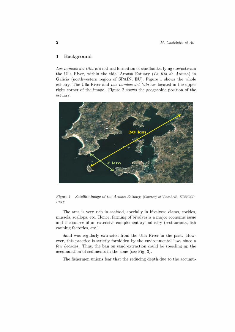
Los Lombos del Ulla is a natural formation of sandbanks, lying downstreamthe Ulla River, within the tidal Arousa Estuary (La Rıa de Arousa) inGalicia (northwestern region of SPAIN, EU). Figure 1 shows the wholeestuary. The Ulla River and Los Lombos del Ulla are located in the upperright corner of the image. Figure 2 shows the geographic position of theestuary.

Figure 1: Satellite image of the Arousa Estuary, [Courtesy of VideaLAB, ETSICCP–

UDC].

The area is very rich in seafood, specially in bivalves: clams, cockles,mussels, scallops, etc. Hence, farming of bivalves is a major economic issueand the source of an extensive complementary industry (restaurants, fishcanning factories, etc.)

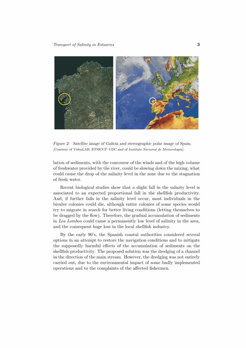
Sand was regularly extracted from the Ulla River in the past. How-ever, this practice is strictly forbidden by the environmental laws since afew decades. Thus, the ban on sand extraction could be speeding up theaccumulation of sediments in the zone (see Fig. 3).

The fishermen unions fear that the reducing depth due to the accumu-

Transport of Salinity in Estuaries 3

Figure 2: Satellite image of Galicia and stereographic polar image of Spain,

[Courtesy of VideaLAB, ETSICCP–UDC and of Instituto Nacional de Meteorologıa].

lation of sediments, with the concourse of the winds and of the high volumeof freshwater provided by the river, could be slowing down the mixing, whatcould cause the drop of the salinity level in the zone due to the stagnationof fresh water.

Recent biological studies show that a slight fall in the salinity level isassociated to an expected proportional fall in the shellfish productivity.And, if further falls in the salinity level occur, most individuals in thebivalve colonies could die, although entire colonies of some species wouldtry to migrate in search for better living conditions (letting themselves tobe dragged by the flow). Therefore, the gradual accumulation of sedimentsin Los Lombos could cause a permanently low level of salinity in the area,and the consequent huge loss in the local shellfish industry.

By the early 90’s, the Spanish coastal authorities considered severaloptions in an attempt to restore the navigation conditions and to mitigatethe supposedly harmful effects of the accumulation of sediments on theshellfish productivity. The proposed solution was the dredging of a channelin the direction of the main stream. However, the dredging was not entirelycarried out, due to the environmental impact of some badly implementedoperations and to the complaints of the affected fishermen.


Figure 3: Los Lombos del Ulla circa 1995, [Courtesy of VideaLAB, ETSICCP–UDC].

In 2002 the Xunta de Galicia (the Regional Government) started todesign a new plan for Los Lombos del Ulla with the following two goals:a) to preserve the shellfish productivity, and b) to restore the navigationconditions in the area. Two actions were initially considered: 1) to dredgea navigation channel (as it had been proposed about a decade before), and2) to dredge the whole area, in order to increase the depth. In fact, thelatter became an unyielding demand of the fishermen unions.

The main objective of this project was the development of a numericalmodel that could be used to evaluate the effect of the proposed actions onthe shellfish productivity of the zone [Navarrina, 2004; Navarrina et Al.,2005].

Furthermore, the information provided by this tool would be used toassess the undesirable side effects of the possible actions (changes in thehydrodynamics of the zone), to evaluate the medium-term and the long-term stability of the sandbanks (the future possible accumulation of sand),and to evaluate the environmental impact of the works (the possible stirringand dragging of solid particles of the seabed and/or their diffusion to otherareas).

2 Mathematical Model

In essence, two coupled models must be considered: a hydrodynamic model(to obtain the velocity field) and an advective-diffusive transport model (topredict the evolution of the salinity level).


Some important issues that must be taken into account are the effectsof the tides (including that the seabed could be exposed) the volume ofwater provided by the Ulla River and the effects of the winds.

The Arousa Estuary can be considered a shallow water domain, sincethe depth is small when compared to the other two spatial dimensions.Therefore the hydrodynamic phenomena can be adequately described bymeans of the shallow water hydrodynamic equations [Peraire et Al., 1986;Scarlatos, 1996].

This is a known 2D model, that is obtained by vertical integration ofthe Navier-Stokes equations [Peraire, 1986]. In essence, in this approachone assumes that the vertically averaged velocity at each point can beconsidered representative of the velocity field in the corresponding verticalcolumn of water.

In a similar way, we expect the vertically averaged salinity at eachpoint to be representative of the salinity field in the corresponding verticalcolumn of water. Thus, the transport of salt can be adequately describedby means of a shallow water type transport model [Fischer et Al., 1979;Holley, 1996; Peraire et Al., 1986; Rutherford, 1994] that is obtained byvertical integration of the advection-diffusion equations [Peraire, 1986].

The registers of salinity in Los Lombos show that the vertical distribu-tion is almost uniform, with a very weak stratification in the area of interest.Hence, it seems that there is no need to implement a multiple-layer modelin this case.

Thus, for each point (x, y), at each time step t, the unknowns to becomputed will be the depth h(x, y, t) = z(x, y, t)− zb(x, y), where z(x, y, t)is the sea surface height and zb(x, y) is the seabed height, the velocity vectorvvvvvvvvvvvvvv(x, y, t) = [vx(x, y, t), vy(x, y, t)]T (vertical average of the horizontal veloc-ity) and the salinity c(x, y, t) (vertical average of the salt concentration).

Then, the whole set of shallow water equations (hydrodynamic andtransport) can be written in a conservative form [Peraire, 1986; Peraire etAl., 1986] as

∂uuuuuuuuuuuuuu

∂t+

∂FFFFFFFFFFFFFF x

∂x+

∂FFFFFFFFFFFFFF y

∂y= RRRRRRRRRRRRRRS +

∂RRRRRRRRRRRRRRDx

∂x+

∂RRRRRRRRRRRRRRDy

∂y, uuuuuuuuuuuuuu =

h

hvx

hvy

hc

, (2.1)


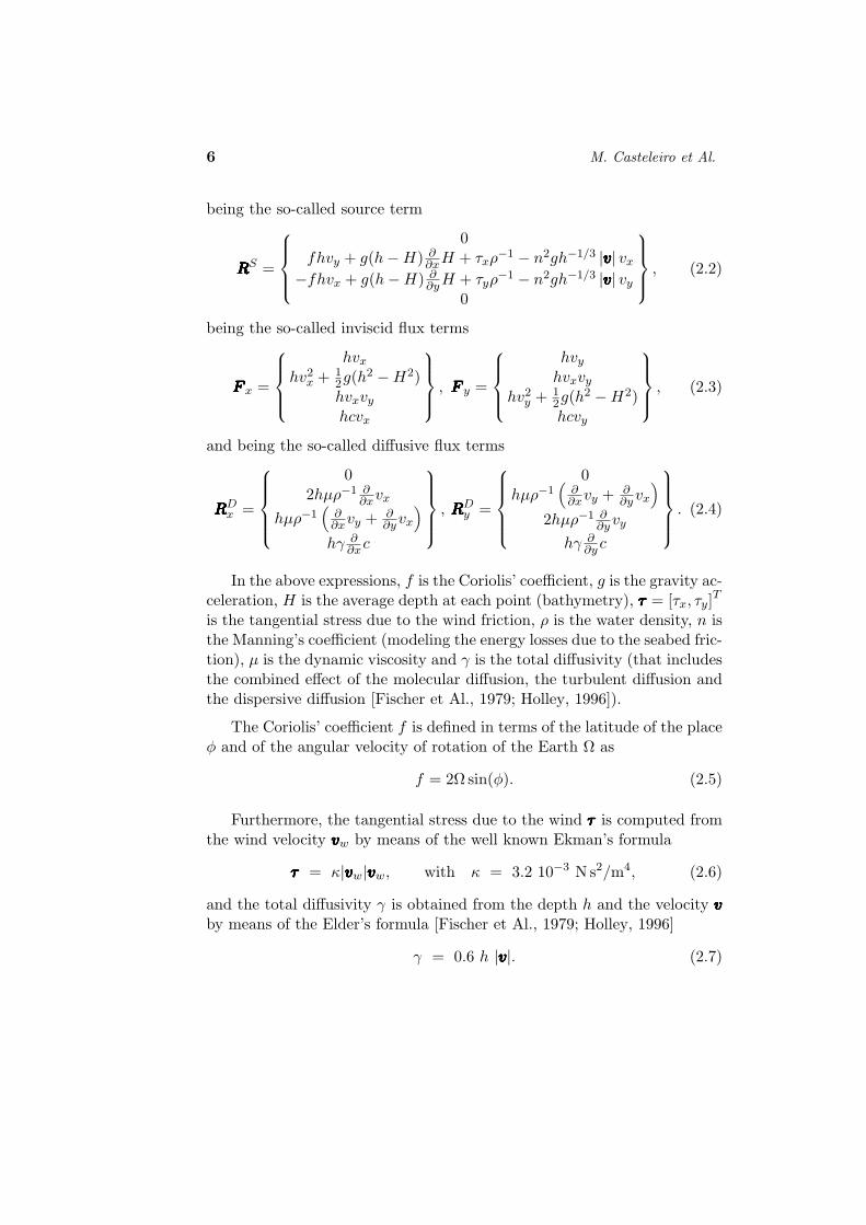
being the so-called source term

RRRRRRRRRRRRRRS =

0

fhvy + g(h − H) ∂∂xH + τxρ−1 − n2gh−1/3 |vvvvvvvvvvvvvv| vx

−fhvx + g(h − H) ∂∂yH + τyρ

−1 − n2gh−1/3 |vvvvvvvvvvvvvv| vy

0

, (2.2)

being the so-called inviscid flux terms

FFFFFFFFFFFFFF x =

hvx

hv2x + 1

2g(h2 − H2)hvxvy

hcvx

, FFFFFFFFFFFFFF y =

hvy

hvxvy

hv2y + 1

2g(h2 − H2)hcvy

, (2.3)

and being the so-called diffusive flux terms

RRRRRRRRRRRRRRDx =

0

2hµρ−1 ∂∂xvx

hµρ−1(

∂∂xvy + ∂

∂yvx

)hγ ∂

∂xc

, RRRRRRRRRRRRRRDy =

0

hµρ−1(

∂∂xvy + ∂

∂yvx

)2hµρ−1 ∂

∂yvy

hγ ∂∂y c

. (2.4)

In the above expressions, f is the Coriolis’ coefficient, g is the gravity ac-celeration, H is the average depth at each point (bathymetry), ττττττττττττττ = [τx, τy]

T

is the tangential stress due to the wind friction, ρ is the water density, n isthe Manning’s coefficient (modeling the energy losses due to the seabed fric-tion), µ is the dynamic viscosity and γ is the total diffusivity (that includesthe combined effect of the molecular diffusion, the turbulent diffusion andthe dispersive diffusion [Fischer et Al., 1979; Holley, 1996]).

The Coriolis’ coefficient f is defined in terms of the latitude of the placeφ and of the angular velocity of rotation of the Earth Ω as

f = 2Ω sin(φ). (2.5)

Furthermore, the tangential stress due to the wind ττττττττττττττ is computed fromthe wind velocity vvvvvvvvvvvvvvw by means of the well known Ekman’s formula

ττττττττττττττ = κ|vvvvvvvvvvvvvvw|vvvvvvvvvvvvvvw, with κ = 3.2 10−3 N s2/m4, (2.6)

and the total diffusivity γ is obtained from the depth h and the velocity vvvvvvvvvvvvvvby means of the Elder’s formula [Fischer et Al., 1979; Holley, 1996]

γ = 0.6 h |vvvvvvvvvvvvvv|. (2.7)


With regard to the boundary conditions, we have three different situa-tions.

In the part of the boundary that corresponds to the mouth of the UllaRiver we can suppose that the flow is super-critical (what precludes the con-ditions in the estuary to influence the upstream flow). Thus, we prescribethe flux and the salinity as

h vvvvvvvvvvvvvvT nnnnnnnnnnnnnn = −hQR

A(h)and c = 0 on the river, (2.8)

where QR is the known volume of flow in the river, A(h) is the area of thewet section of the river and nnnnnnnnnnnnnn is the external normal to the boundary. Thesalinity c is prescribed to be null, since the river flows fresh water into theestuary.

In the part of the boundary that corresponds to the sea we can supposethat the flow is sub-critical. Thus, we prescribe the depth and the salinityas

z = zS(t) + ∆zS and c = cS on the sea, (2.9)

where zS(t) is the prescribed depth due to the tide harmonics and ∆zS

is the so-called meteorological tide. The meteorological tide is the rise orthe fall of the surface level during a storm (due to the wind that blows onthe whole fetch). It can be obtained from the corresponding measures andrecords of the seaports authorities.

Finally, we can state that both the flux of water and the flux of salt arenull in the direction nnnnnnnnnnnnnn of the normal to the shore, what gives

h vvvvvvvvvvvvvvT nnnnnnnnnnnnnn = 0 and h gradgradgradgradgradgradgradgradgradgradgradgradgradgradT (c)nnnnnnnnnnnnnn = 0 on the shore. (2.10)

3 Numerical Model

The above stated problem must be solved numerically. In order to do so,we will use the Finite Element Method. More specifically, we will solvethe problem by means of a second order Taylor-Galerkin (TG-2) approach[Donea et Al., 2003; Peraire, 1986; Peraire et Al., 1986; Zienkiewicz et Al.,2000].


3.1 Derivation of the TG-2 Formulation

In order to derive the Taylor-Galerkin formulation, we first write a Taylor’sexpansion in the time coordinate of the unknown uuuuuuuuuuuuuu

uuuuuuuuuuuuuu∣∣∣t=tn+1

= uuuuuuuuuuuuuu∣∣∣t=tn

+∆t

1!∂uuuuuuuuuuuuuu

∂t

∣∣∣t=tn

+∆t2

2!∂2uuuuuuuuuuuuuu

∂t2

∣∣∣t=tn

+ O(∆t3)


+ ∆t

[∂uuuuuuuuuuuuuu

∂t+

∆t

2∂2uuuuuuuuuuuuuu

∂t2

]∣∣∣t=tn

+ O(∆t3).(3.1)

Then we can rewrite the above expansion as

uuuuuuuuuuuuuu∣∣∣t=tn+1


+ ∆t wwwwwwwwwwwwww∣∣∣t=tn

+ O(∆t3), (3.2)

where

wwwwwwwwwwwwww =

[∂uuuuuuuuuuuuuu

∂t+

∆t

2∂2uuuuuuuuuuuuuu

∂t2

]. (3.3)

By taking into account the differential equation (2.1) we can write

∂uuuuuuuuuuuuuu

∂t= RRRRRRRRRRRRRRS−

(∂FFFFFFFFFFFFFF x

∂x+

∂FFFFFFFFFFFFFF y

∂y

)+

(∂RRRRRRRRRRRRRRD

x

∂x+

∂RRRRRRRRRRRRRRDy

∂y

),

∂2uuuuuuuuuuuuuu

∂t2=

∂

∂tRRRRRRRRRRRRRRS − ∂

∂t


∂x+

∂FFFFFFFFFFFFFF y

∂y

)+

∂

∂t

(∂RRRRRRRRRRRRRRD

x

∂x+

∂RRRRRRRRRRRRRRDy

∂y

)

= RRRRRRRRRRRRRRS−


∂x+

∂FFFFFFFFFFFFFF y

∂y

)+

∂RRRRRRRRRRRRRRDx

∂x+

∂RRRRRRRRRRRRRRDy

∂y

.

(3.4)

Therefore, we can rewrite (3.3) as

wwwwwwwwwwwwww =

[∂uuuuuuuuuuuuuu

∂t+

∆t

2∂2uuuuuuuuuuuuuu

∂t2

]= bbbbbbbbbbbbbb −

(∂AAAAAAAAAAAAAAx

∂x+

∂AAAAAAAAAAAAAAy

∂y

), (3.5)

being

bbbbbbbbbbbbbb = RRRRRRRRRRRRRRS +∆t

2RRRRRRRRRRRRRR

S,

AAAAAAAAAAAAAAx =(FFFFFFFFFFFFFF x +

∆t

2FFFFFFFFFFFFFF x

)−(RRRRRRRRRRRRRRD

x +∆t

2RRRRRRRRRRRRRR

Dx

),

AAAAAAAAAAAAAAy =(FFFFFFFFFFFFFF y +

∆t

2FFFFFFFFFFFFFF y

)−(RRRRRRRRRRRRRRD

y +∆t

2RRRRRRRRRRRRRR

Dy

).

(3.6)


Applying the Weighted Residuals Method in the spatial coordinates to(3.5) yields∫∫

(x,y)∈Ω$

(wwwwwwwwwwwwww −

[bbbbbbbbbbbbbb −

(∂AAAAAAAAAAAAAAx

∂x+

∂AAAAAAAAAAAAAAy

∂y

)])dΩ = 0 ∀$, (3.7)

that can be rewritten as∫∫(x,y)∈Ω

$ wwwwwwwwwwwwww dΩ =∫∫

(x,y)∈Ω$ bbbbbbbbbbbbbb dΩ

−∫∫

(x,y)∈Ω$

(∂AAAAAAAAAAAAAAx

∂x+

∂AAAAAAAAAAAAAAy

∂y

)dΩ ∀$.

(3.8)

In the previous expression we can replace

$

(∂AAAAAAAAAAAAAAx

∂x+

∂AAAAAAAAAAAAAAy

∂y

)=[

∂

∂x($ AAAAAAAAAAAAAAx) +

∂

∂y($ AAAAAAAAAAAAAAy)

]−[∂$

∂xAAAAAAAAAAAAAAx +

∂$

∂yAAAAAAAAAAAAAAy

],

(3.9)

and we can define

AAAAAAAAAAAAAA˜ = [AAAAAAAAAAAAAAx AAAAAAAAAAAAAAy ] , gradgradgradgradgradgradgradgradgradgradgradgradgradgradT ($) =

∂$

∂x

∂$

∂y

. (3.10)

Now we can write[∂$

∂xAAAAAAAAAAAAAAx +

∂$

∂yAAAAAAAAAAAAAAy

]= AAAAAAAAAAAAAA˜ gradgradgradgradgradgradgradgradgradgradgradgradgradgrad($), (3.11)

and by applying the divergence theorem∫∫(x,y)∈Ω

[∂

∂x($ AAAAAAAAAAAAAAx) +

∂

∂y($ AAAAAAAAAAAAAAy)

]dΩ =

∫(x,y)∈∂Ω

$ AAAAAAAAAAAAAA˜ nnnnnnnnnnnnnn d∂Ω, (3.12)

we finally obtain the variational form of the problem∫∫(x,y)∈Ω

$ wwwwwwwwwwwwww dΩ =∫∫

(x,y)∈Ω$ bbbbbbbbbbbbbb dΩ

+∫∫

(x,y)∈ΩAAAAAAAAAAAAAA˜ gradgradgradgradgradgradgradgradgradgradgradgradgradgrad($) dΩ

−∫(x,y)∈∂Ω

$ AAAAAAAAAAAAAA˜ nnnnnnnnnnnnnn d∂Ω ∀$.

(3.13)


Now, if we discretize the trial functions in the form

uuuuuuuuuuuuuu(x, y, t) =∑I

uuuuuuuuuuuuuuI(t)φI(x, y),

wwwwwwwwwwwwww(x, y, t) =∑I

wwwwwwwwwwwwwwI(t)φI(x, y),(3.14)

and the test functions in the form

$(x, y, t) =∑J

ββββββββββββββJ(t)$J(x, y), (3.15)

we obtain the discretized variational form∑I

[∫∫(x,y)∈Ω

$J φI dΩ

]wwwwwwwwwwwwwwI =

∫∫(x,y)∈Ω

[$J bbbbbbbbbbbbbb + AAAAAAAAAAAAAA˜ gradgradgradgradgradgradgradgradgradgradgradgradgradgrad($J)] dΩ

−∫(x,y)∈∂Ω

$J AAAAAAAAAAAAAA˜ nnnnnnnnnnnnnn d∂Ω ∀J.

(3.16)

If we now choose the Galerkin Method.

$J(x, y) = φJ(x, y) (3.17)

we finally get the second-order Taylor-Galerkin expressions.

3.2 Implementation of the TG-2 Algorithm

In essence, at each time step the following linear system of equations issolved (space integration)∑

I

[MJI ] wwwwwwwwwwwwwwI(tn) = ffffffffffffffJ∣∣∣t=tn

, with

[MJI ] =

[∫∫(x,y)∈Ω

φJ φI dΩ

]and

ffffffffffffffJ =

∫∫(x,y)∈Ω

[φJ bbbbbbbbbbbbbb + AAAAAAAAAAAAAA˜ gradgradgradgradgradgradgradgradgradgradgradgradgradgrad(φJ)] dΩ −∫(x,y)∈∂Ω

φJ AAAAAAAAAAAAAA˜ nnnnnnnnnnnnnn d∂Ω

.

(3.18)Then, the solution is updated (time integration) by neglecting third ordererrors, what gives the second order accurate expression

uuuuuuuuuuuuuuI(tn+1) = uuuuuuuuuuuuuuI(tn) + ∆t wwwwwwwwwwwwwwI(tn). (3.19)


The coefficients matrix in system (3.18) is the so-called “mass matrix”.This linear system can be solved by using a Diagonal Preconditioned Con-jugate Gradient algorithm without assembling the global matrix. Alterna-tively, the solution to (3.18) can be approximated by using the so-calleddiagonal lumped mass matrix [Peraire et Al., 1986]. This has been theprocedure that was finally used in this project.

4 Discretization and Bathymetry

Although the area of interest (Los Lombos del Ulla) is relatively small, weare forced to analyze the whole estuary (see Fig. 1) in order to impose thesea boundary conditions far enough from the area of interest, and in order totake into account the influence of the whole estuary in the hydrodynamics.

The estuary was discretized by the Gen4u mesh generator [Sarrate,1996; Sarrate et Al., 2000, 2001; Soage, 2005] in 30970 isoparametric quad-rangular elements of 4 nodes, what yields 120424 degrees of freedom (30106nodes times 4 d.o.f. per node) at each time step (see Fig. 4).

Approximately half of the total elements (14979) are placed in Los Lom-bos del Ulla while the rest are spread in the rest of the estuary, what isthe most extensive part. The size of the elements gradually grows as wemove away from Los Lombos. Thus, we seek more precise results in thearea of interest. But, also, we try to avoid the stability conditions [Peraireet Al., 1986] to become excessively restrictive, since the largest elementsare located in the deepest areas (where the velocity of propagation of thegravity waves is higher).

The actual bathymetry of the whole estuary was obtained from somemeasurements specifically made in Los Lombos during 2002, from the chartsof the estuary and from the available topographic data of the shore [Navar-rina, 2004] (see Fig. 4).

The bathymetry that corresponds to the first possible action (dredg-ing a navigation channel) was obtained from the actual bathymetry bydropping the corresponding values of the seabed height down to the level−1.5 m. This action implies the dredging of 614, 651.24 m3 of solids. Thebathymetry that corresponds to the second possible action (general dredg-ing of Los Lombos) was obtained from the actual bathymetry by droppingthe corresponding values of the seabed height down to the level −0.5 m,


Figure 4: GEN4U discretization of the whole estuary (left). Actual bathymetry

(right).

but limiting the drop to 0.75 m in each point at the most [Navarrina, 2004].This action implies the dredging of 3, 876, 503.49 m3 of solids.

5 Program of Simulations

Two types of simulations were carried out: 28 days simulations in normalconditions (NC) and 2 days simulations in extreme conditions (EC) [Navar-rina, 2004]. The 28 days simulations compare the results obtained for theactual bathymetry (i.e., the current situation) with the results predictedfor each one of the two possible actions (dredging a navigation channel anddredging the whole area of Los Lombos). The second option was discardedafter analyzing these results. Thus, the 2 days simulations only comparethe results obtained for the current bathymetry with the results predictedfor the first possible action (dredging a navigation channel). In the NCsimulations we considered the average volume of water (QMED

R = 56 m3/s)in the Ulla River, and the average velocity wind (vvvvvvvvvvvvvvMED

W = 4.8 m/s) blow-ing in the dominant direction (202o S–SW) without meteorological tide(∆zS = 0 m). On the other hand, 5 different extreme conditions were de-fined: Southwest storm (EC#1), flood condition (EC#2), Southwest storm


and flood condition (EC#3), Northeast storm and flood condition (EC#4)and Northeast storm (EC#5). In the EC#2, EC#3 and EC#4 simulationswe considered the flood volume of water (QMAX

R = 300 m3/s) in the UllaRiver. In the other ones (EC#1, EC#5) we considered the average volumeof water (QMED

R ) in the Ulla River. In the EC#1 and EC#3 simulationswe considered the maximum velocity wind (vMAX

W = 15.0 m/s) blowingin the most adverse direction (210o SW) with positive meteorological tide(∆zS = 0.15 m). In the EC#4 and EC#5 simulations we considered themaximum velocity wind (vMAX

W ) blowing in NE direction (30o NE) withnegative meteorological tide (∆zS = −0.15 m). In the remaining simulation(EC#2) we considered the average velocity wind (vMED

W ) blowing in thedominant direction (202o S–SW) without meteorological tide (∆zS = 0 m).

We took the following values for the physical constants of the problem:Ω = 2π/86164.09 rad/s, φ = 43o 35′ 58′′, g = 9.81 m/s2, ρ = 103 Kg/m3,n = 0.0425 s/m1/3, cS = 0.035 and µ = 50 Kg/ms, where the latitude φcorresponds to the Vilagarcıa de Arousa Harbour.

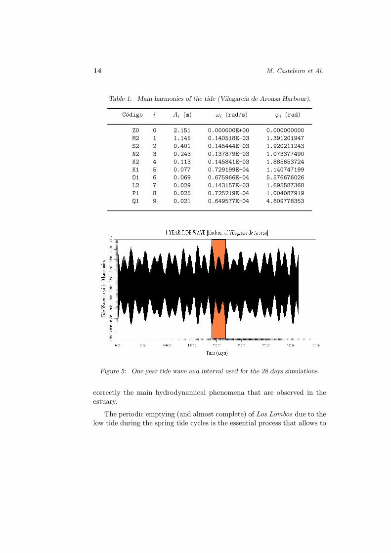
Finally, the tide was modeled by adding up the first 10 harmonics (n =9) of the corresponding Fourier series, as

zS(t) =n∑

i=0

Ai cos(ωit + ϕi), (5.1)

where the amplitude (Ai), the angular frequency (ωi) and the phase (ϕi) ofeach harmonic (i) have been obtained from the Spanish seaports authoritywebsite [Ente Publico Puertos del Estado, 2004] (see table 1).

Fig. 5 shows the one year tide wave and the 28 days window that wasused for the NC simulations.

Fig. 6 shows the 28 days tide wave and the 2 days window that wereused for the NC and for the EC simulations.

6 Analysis of Results and Conclusions

The numerical results of the model have been compared with data givenby the experts in the hydrodynamics of the area, with measurements per-formed during the project and with computed results obtained with simplermodels. The results agree with the available data and the model predicts


Table 1: Main harmonics of the tide (Vilagarcıa de Arousa Harbour).

Codigo i Ai (m) ωi (rad/s) ϕi (rad)

Z0 0 2.151 0.000000E+00 0.000000000M2 1 1.145 0.140518E-03 1.391201947S2 2 0.401 0.145444E-03 1.920211243N2 3 0.243 0.137879E-03 1.073377490K2 4 0.113 0.145841E-03 1.885653724K1 5 0.077 0.729199E-04 1.140747199O1 6 0.069 0.675966E-04 5.576676026L2 7 0.029 0.143157E-03 1.695587368P1 8 0.025 0.725219E-04 1.004087919Q1 9 0.021 0.649577E-04 4.809778353

Figure 5: One year tide wave and interval used for the 28 days simulations.

correctly the main hydrodynamical phenomena that are observed in theestuary.

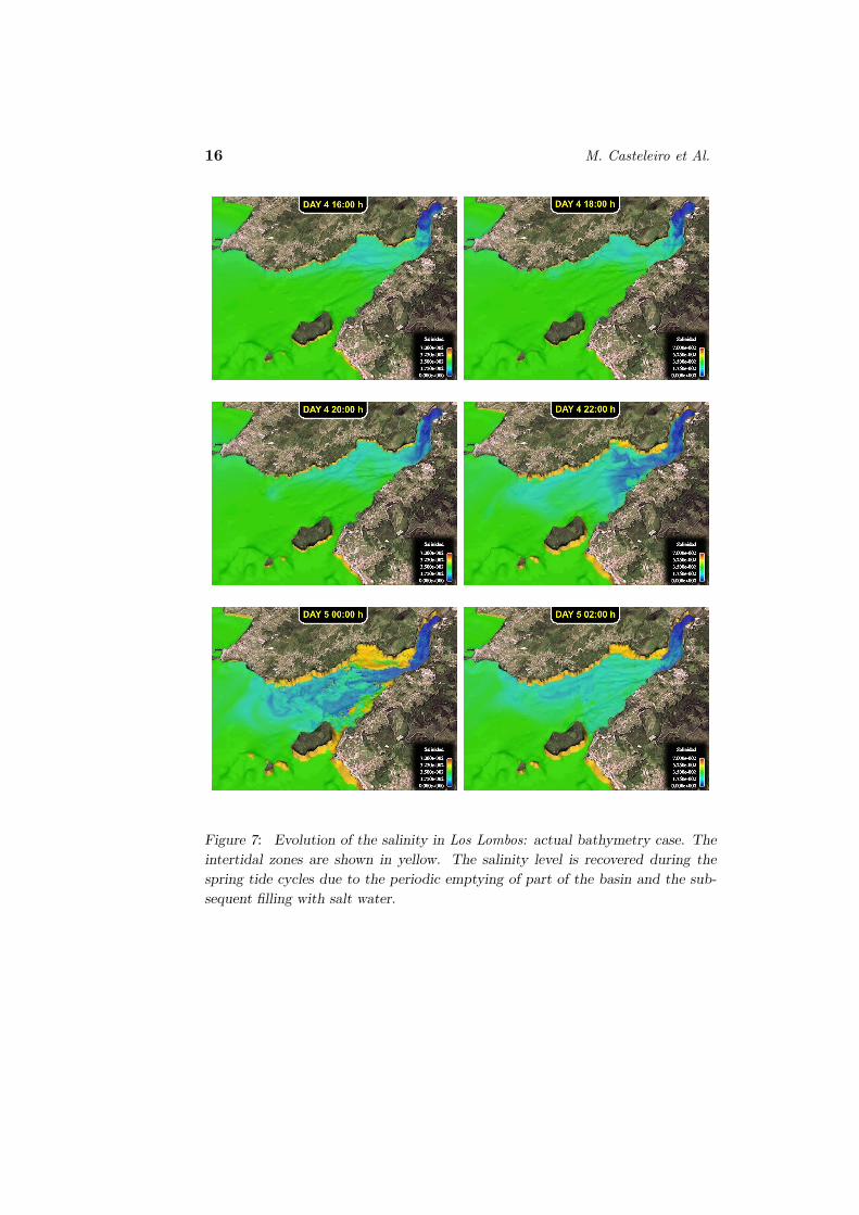
The periodic emptying (and almost complete) of Los Lombos due to thelow tide during the spring tide cycles is the essential process that allows to


Figure 6: 28 days tide wave and subinterval used for the 2 days simulations.

maintain the average level of salinity in the area (see Fig. 7). During theneap tide cycles, the salinity level inexorably falls due to the continuouscontribution of freshwater from the river. However, the salinity level isrecovered during the spring tide cycles, due to the emptying of an importantpart of the basin and the periodic contribution of salt water from the sea.For this reason, we absolutely advised against a general dredging of LosLombos. As it is observed in the simulations, a general dredging causes animportant decrease in the average salinity level in all the area (see Fig. 8).

However, the dredging of a channel does not significantly modify thesalinity level in Los Lombos. Thus, the shellfish production of the areawould not be substantially affected, while the navigation conditions in thearea could be improved.

The presented model contributes to know the marine habitat. It showshow important are the different processes involved in the hydrodynamicsof an estuary. It provides useful and accurate information that can be usedto predict the migration of the shellfish colonies depending on the salinitylevel and on the currents. And it allows to predict the effects of CivilEngineering public works and other human actions (dredging, spillings,etc.) and to evaluate their environmental impact.


Figure 7: Evolution of the salinity in Los Lombos: actual bathymetry case. The

intertidal zones are shown in yellow. The salinity level is recovered during the

spring tide cycles due to the periodic emptying of part of the basin and the sub-

sequent filling with salt water.


Figure 8: Evolution of the salinity in Los Lombos: general dredging case. The

intertidal zones are in shown in yellow. The salinity level is not recovered during

the spring tide cycles, since the beneficial effects of the periodic emptying of part

of the basin are no longer present.


Acknowledgements

This work has been partially supported by the Consellerıa de Pesca of theXunta de Galicia by means of a research contract between the FundacionCETMAR and the Fundacion de la Ingenierıa Civil de Galicia, by Grants# PGDIT01PXI11802PR and # PGDIT03PXIC11802PN of the DXID–CIIC of the Xunta de Galicia, by Grant # DPI-2002-00297 of the SGPI–DGI of the Ministerio de Ciencia y Tecnologıa, and by research fellowshipsof the Universidad de A Coruna and the Fundacion de la Ingenierıa Civilde Galicia.

References

Donea J. and Huerta A. (2003). Finite Element Methods for Flow Prob-lems. John Wiley & Sons, Chichester.

Ente Publico Puertos del Estado (2004). Web de Puertos del Estado<http://www.puertos.es>. Ministerio de Fomento, Spain.

Fischer H.B. et Al. (1979). Mixing in Inland and Coastal Waters. Aca-demic Press Inc., Orlando.

Holley E.R. (1996). Diffusion and Dispersion. In V.P. Singh andW.H. Hager, eds., Environmental Hydraulics, pp. 111–151. Kluwer Aca-demic Publishers, Dordrecht.

Navarrina F. (2004). Modelo Numerico de los Lombos del Ulla: InformeFinal . Technical Report, Fundacion de la Ingenierıa Civil de Galicia—Universidad de A Coruna, A Coruna, Spain.

Navarrina F., Colominas I., Casteleiro M., Cueto-Felgueroso L., Gomez H., Fe J. and Soage A. (2005). Analysisof Hydrodynamic and Transport Phenomena in the Rıa de Arousa:A Numerical Model for High Environmental Impact Estuaries. InS.K. Chakrabarti, S. Hernandez and C.A. Brebbia, eds., Fluid StructureInteraction and Moving Boundary Problems, pp. 583–593. WIT Press,Southampton.

Peraire J. (1986). A Finite Element Method for convection dominatedflows. PhD Thesis, University College of Swansea, Wales, UK.


Peraire J., Zienkiewicz O.C. and Morgan K. (1986). Shallow wa-ter problems: a general explicit formulation. International Journal forNumerical Methods in Engineering , 22:547–574.

Rutherford J.C. (1994). River Mixing . John Wiley & Sons, Chichester.

Sarrate J. (1996). Modelizacion numerica de la interaccion fluido-solidorıgido: desarrollo de algoritmos, generacion de mallas y adaptabilidad .PhD Thesis, Universitat Politecnica de Catalunya, Barcelona, Spain.

Sarrate J. and Huerta A. (2000). Efficient unstructured quadrilateralmesh generation. International Journal for Numerical Methods in Engi-neering , 49:1327–1350.

Sarrate J. and Huerta A. (2001). Manual de Gen4u (Version 2.1). Tech-nical Report, LaCaN, Universitat Politecnica de Catalunya, Barcelona,Spain.

Scarlatos P.D. (1996). Estuarine Hydraulics. In V.P. Singh andW.H. Hager, eds., Environmental Hydraulics, pp. 289–348. Kluwer Aca-demic Publishers, Dordrecht.

Soage A. (2005). Simulacion numerica del comportamiento hidrodinamicoy de evolucion de la salinidad en zonas costeras de gran impacto ambien-tal: aplicacion a la Rıa de Arousa. MSc Thesis, Escuela Tecnica Superiorde Ingenieros de Caminos, Canales y Puertos, Universidad de A Coruna,A Coruna, Spain.

Zienkiewicz O.C. and Taylor R.L. (2000). The Finite Element Method,Vol. III: Fluid Dynamics. Butterworth-Heinemann, Oxford.

Documents

A Mathematical and Numerical Model for the Transport of