Steel heat treating: mathematical modelling and numerical

Advances in Science, Technology and Engineering Systems JournalVol. 2, No. 5, 55-62 (2017)

www.astesj.comProceedings of International Conference on Applied Mathematics

(ICAM’2017), Taza, Morocco

ASTES JournalISSN: 2415-6698

Steel heat treating: mathematical modelling and numericalsimulation of a problem arising in the automotive industryJose Manuel Dıaz Moreno1, Concepcion Garcıa Vazquez1, Marıa Teresa Gonzalez Montesinos2,Francisco Ortegon Gallego*,1, Giuseppe Viglialoro3

1Departamento de Matematicas, Facultad de Ciencias, Universidad de Cadiz, 11510 Puerto Real, SPAIN,[email protected], [email protected], [email protected].

2Departamento de Matematica Aplicada I, ETS de Ingenierıa Informatica, Universidad de Sevilla, 41012 Sevilla,SPAIN, [email protected].

3Dipartimento di Matematica ed Informatica, Universita degli Studi di Cagliari, viale Merello 92 – 09123Cagliari, ITALY, [email protected].

A R T I C L E I N F O A B S T R A C TArticle history:Received: 10 June, 2017Accepted: 15 July, 2017Online: 10 December, 2017

We describe a mathematical model for the industrial heating and cooling processes of a steel workpiece representing the steering rack of an automobile. The goal of steel heat treating is to provide a hardened surface on critical parts of the workpiece while keeping the rest soft and ductile in order to reduce fatigue. The high hardness is due to the phase transformation of steel accompanying the rapid cooling. This work takes into account both heating-cooling stage and viscoplastic model. Once the general mathematical formulation is derived, we can perform some numerical simulations.

Keywords :Steel hardeningPhase transitionsPotential Maxwell equationsNumerical SimulationsFinite Element Methods

1 Introduction

In the automative industry, many workpieces suchgears, bearings, racks and pinions, are made of steel.Steel is an alloy of iron and carbon. Generally, indus-trial steel has a carbon content up to about 2 wt%.Other alloying elements may be present, such as Crand V in tools steels, or Si, Mn, Ni and Cr in stain-less steels. Most structural components in mechanicalengineering are made of steel. Certain of these com-ponents, such as toothed wheels, bevel gears, pinionsand so on, engaged each others in order to transmitsome kind of (rotational or longitudinal) movement.In this situation, the contact surfaces of these compo-nents are particularly stressed. The goal of heat treat-ing of steel is to attain a satisfactory hardness. Priorto heat treating, steel is a soft and ductile material.Without a hardening treatment, and due to the sur-face stresses, the gear teeth will soon get damaged andthey will no longer engage correctly.

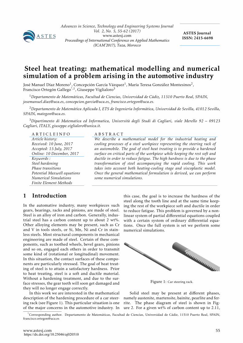
In this work we are interested in the mathematicaldescription of the hardening procedure of a car steer-ing rack (see Figure 1). This particular situation is oneof the major concerns in the automotive industry. In

this case, the goal is to increase the hardness of thesteel along the tooth line and at the same time keep-ing the rest of the workpiece soft and ductile in orderto reduce fatigue. This problem is governed by a non-linear system of partial differential equations coupledwith a certain system of ordinary differential equa-tions. Once the full system is set we perform somenumerical simulations.

Figure 1: Car steering rack.

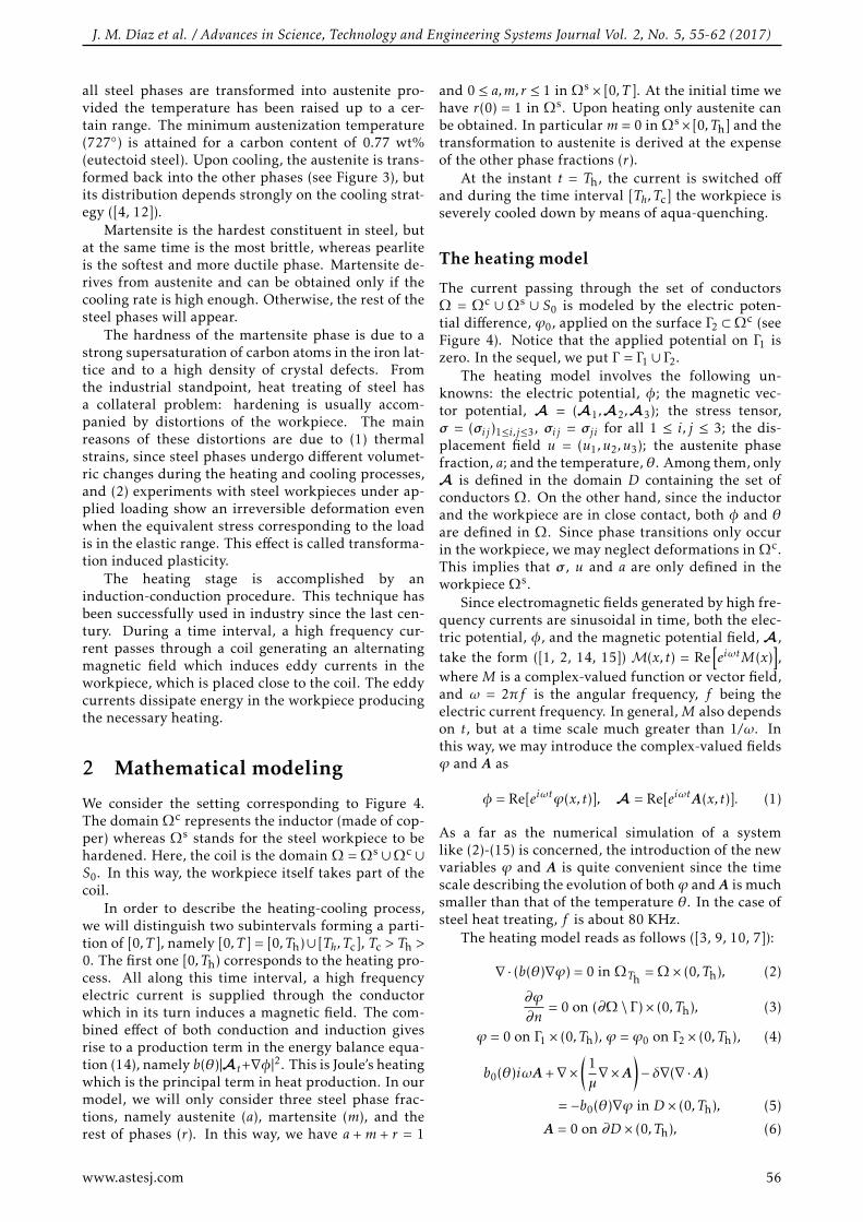
Solid steel may be present at different phases,namely austenite, martensite, bainite, pearlite and fer-rite. The phase diagram of steel is shown in Fig-ure 2. For a given wt% of carbon content up to 2.11,

*Corresponding author. Departamento de Matematicas, Facultad de Ciencias, Universidad de Cadiz, 11510 Puerto Real, SPAIN,[email protected]

www.astesj.com 55https://dx.doi.org/10.25046/aj020510

www.astesj.com

J. M. Dıaz et al. / Advances in Science, Technology and Engineering Systems Journal Vol. 2, No. 5, 55-62 (2017)

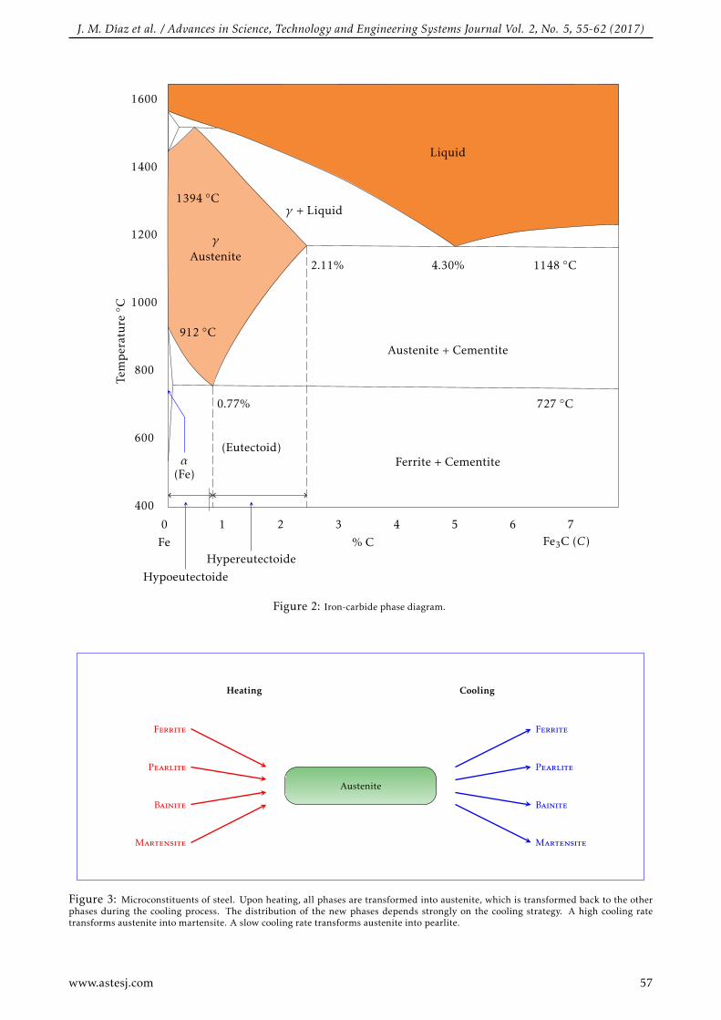
all steel phases are transformed into austenite pro-vided the temperature has been raised up to a cer-tain range. The minimum austenization temperature(727) is attained for a carbon content of 0.77 wt%(eutectoid steel). Upon cooling, the austenite is trans-formed back into the other phases (see Figure 3), butits distribution depends strongly on the cooling strat-egy ([4, 12]).

Martensite is the hardest constituent in steel, butat the same time is the most brittle, whereas pearliteis the softest and more ductile phase. Martensite de-rives from austenite and can be obtained only if thecooling rate is high enough. Otherwise, the rest of thesteel phases will appear.

The hardness of the martensite phase is due to astrong supersaturation of carbon atoms in the iron lat-tice and to a high density of crystal defects. Fromthe industrial standpoint, heat treating of steel hasa collateral problem: hardening is usually accom-panied by distortions of the workpiece. The mainreasons of these distortions are due to (1) thermalstrains, since steel phases undergo different volumet-ric changes during the heating and cooling processes,and (2) experiments with steel workpieces under ap-plied loading show an irreversible deformation evenwhen the equivalent stress corresponding to the loadis in the elastic range. This effect is called transforma-tion induced plasticity.

The heating stage is accomplished by aninduction-conduction procedure. This technique hasbeen successfully used in industry since the last cen-tury. During a time interval, a high frequency cur-rent passes through a coil generating an alternatingmagnetic field which induces eddy currents in theworkpiece, which is placed close to the coil. The eddycurrents dissipate energy in the workpiece producingthe necessary heating.

2 Mathematical modeling

We consider the setting corresponding to Figure 4.The domain Ωc represents the inductor (made of cop-per) whereas Ωs stands for the steel workpiece to behardened. Here, the coil is the domain Ω = Ωs ∪Ωc ∪S0. In this way, the workpiece itself takes part of thecoil.

In order to describe the heating-cooling process,we will distinguish two subintervals forming a parti-tion of [0,T ], namely [0,T ] = [0,Th)∪ [Th,Tc], Tc > Th >0. The first one [0,Th) corresponds to the heating pro-cess. All along this time interval, a high frequencyelectric current is supplied through the conductorwhich in its turn induces a magnetic field. The com-bined effect of both conduction and induction givesrise to a production term in the energy balance equa-tion (14), namely b(θ)|At+∇φ|2. This is Joule’s heatingwhich is the principal term in heat production. In ourmodel, we will only consider three steel phase frac-tions, namely austenite (a), martensite (m), and therest of phases (r). In this way, we have a +m + r = 1

and 0 ≤ a,m,r ≤ 1 in Ωs × [0,T ]. At the initial time wehave r(0) = 1 in Ωs. Upon heating only austenite canbe obtained. In particular m = 0 in Ωs× [0,Th] and thetransformation to austenite is derived at the expenseof the other phase fractions (r).

At the instant t = Th, the current is switched offand during the time interval [Th,Tc] the workpiece isseverely cooled down by means of aqua-quenching.

The heating model

The current passing through the set of conductorsΩ = Ωc ∪Ωs ∪ S0 is modeled by the electric poten-tial difference, ϕ0, applied on the surface Γ2 ⊂Ωc (seeFigure 4). Notice that the applied potential on Γ1 iszero. In the sequel, we put Γ = Γ1 ∪ Γ2.

The heating model involves the following un-knowns: the electric potential, φ; the magnetic vec-tor potential, A = (A1,A2,A3); the stress tensor,σ = (σij )1≤i,j≤3, σij = σji for all 1 ≤ i, j ≤ 3; the dis-placement field u = (u1,u2,u3); the austenite phasefraction, a; and the temperature, θ. Among them, onlyA is defined in the domain D containing the set ofconductors Ω. On the other hand, since the inductorand the workpiece are in close contact, both φ and θare defined in Ω. Since phase transitions only occurin the workpiece, we may neglect deformations in Ωc.This implies that σ , u and a are only defined in theworkpiece Ωs.

Since electromagnetic fields generated by high fre-quency currents are sinusoidal in time, both the elec-tric potential, φ, and the magnetic potential field,A,take the form ([1, 2, 14, 15]) M(x, t) = Re

[eiωtM(x)

],

where M is a complex-valued function or vector field,and ω = 2πf is the angular frequency, f being theelectric current frequency. In general,M also dependson t, but at a time scale much greater than 1/ω. Inthis way, we may introduce the complex-valued fieldsϕ and A as

φ = Re[eiωtϕ(x, t)], A = Re[eiωtA(x, t)]. (1)

As a far as the numerical simulation of a systemlike (2)-(15) is concerned, the introduction of the newvariables ϕ and A is quite convenient since the timescale describing the evolution of bothϕ andA is muchsmaller than that of the temperature θ. In the case ofsteel heat treating, f is about 80 KHz.

The heating model reads as follows ([3, 9, 10, 7]):

∇ · (b(θ)∇ϕ) = 0 in ΩTh= Ω× (0,Th), (2)

∂ϕ

∂n= 0 on (∂Ω \ Γ )× (0,Th), (3)

ϕ = 0 on Γ1 × (0,Th), ϕ = ϕ0 on Γ2 × (0,Th), (4)

b0(θ)iωA+∇×(

1µ∇×A

)− δ∇(∇ ·A)

= −b0(θ)∇ϕ in D × (0,Th), (5)

A = 0 on ∂D × (0,Th), (6)

www.astesj.com 56

http://www.astesj.com


Tem

per

atu

re C

400

600

800

1000

1200

1400

1600

0 1 2 3 4 5 6 7

Fe % C Fe3C (C)

Hypoeutectoide

Hypereutectoide

α(Fe)

Ferrite + Cementite

727 C

1148 C

912 C

1394 C

0.77%

(Eutectoid)

2.11% 4.30%

Austenite + Cementite

Liquid

γ + Liquid

γAustenite

Figure 2: Iron-carbide phase diagram.

Ferrite

Pearlite

Bainite

Martensite

Austenite

Ferrite

Pearlite

Bainite

Martensite

Heating Cooling

Figure 3: Microconstituents of steel. Upon heating, all phases are transformed into austenite, which is transformed back to the otherphases during the cooling process. The distribution of the new phases depends strongly on the cooling strategy. A high cooling ratetransforms austenite into martensite. A slow cooling rate transforms austenite into pearlite.

www.astesj.com 57



Ωs (steel)

Ωc (copper) Ωc

Γ1 Γ2

S0S0

D

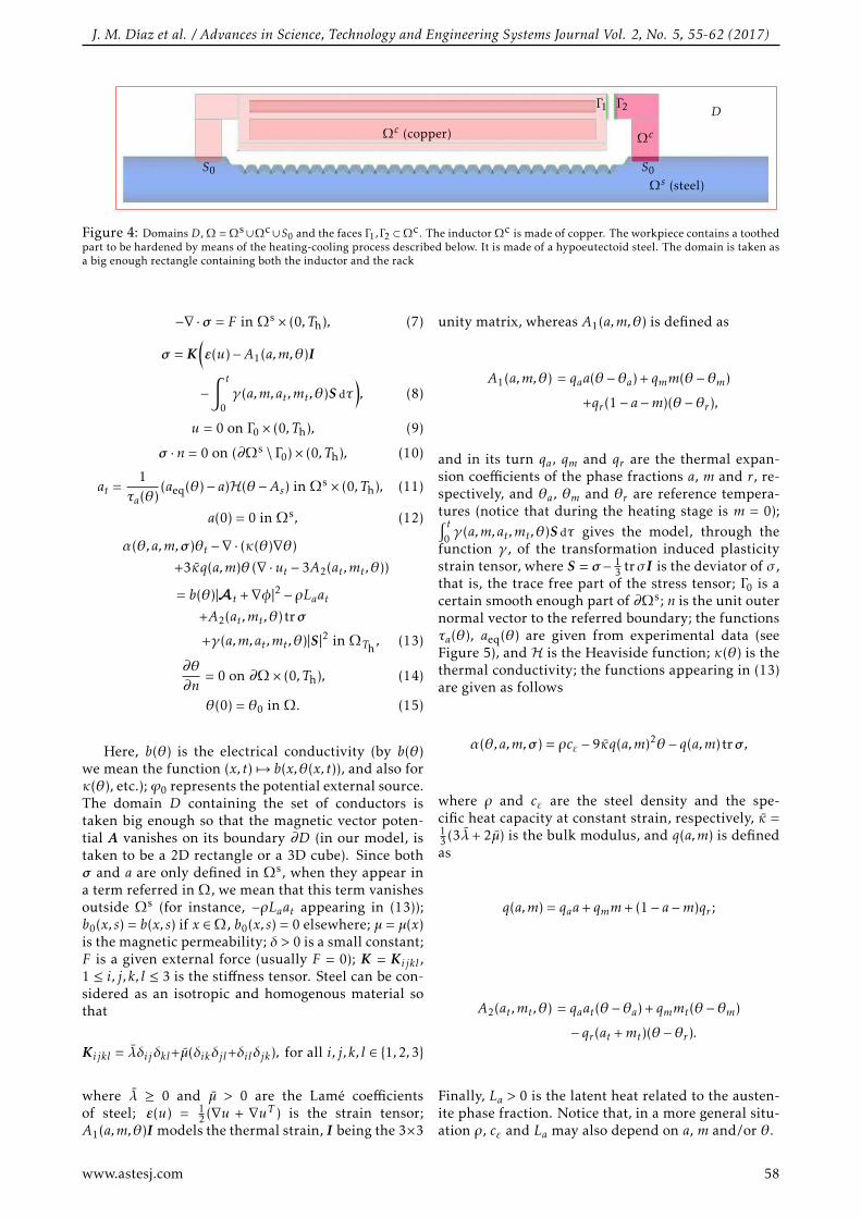
Figure 4: Domains D, Ω = Ωs∪Ωc∪S0 and the faces Γ1,Γ2 ⊂Ωc. The inductor Ωc is made of copper. The workpiece contains a toothedpart to be hardened by means of the heating-cooling process described below. It is made of a hypoeutectoid steel. The domain is taken asa big enough rectangle containing both the inductor and the rack

−∇ ·σ = F in Ωs × (0,Th), (7)

σ =K(ε(u)−A1(a,m,θ)I

−∫ t

0γ(a,m,at ,mt ,θ)S dτ

), (8)

u = 0 on Γ0 × (0,Th), (9)

σ ·n = 0 on (∂Ωs \ Γ0)× (0,Th), (10)

at =1

τa(θ)(aeq(θ)− a)H(θ −As) in Ωs × (0,Th), (11)

a(0) = 0 in Ωs, (12)

α(θ,a,m,σ )θt −∇ · (κ(θ)∇θ)

+3κq(a,m)θ (∇ ·ut − 3A2(at ,mt ,θ))

= b(θ)|At +∇φ|2 − ρLaat+A2(at ,mt ,θ) trσ

+γ(a,m,at ,mt ,θ)|S|2 in ΩTh, (13)

∂θ∂n

= 0 on ∂Ω× (0,Th), (14)

θ(0) = θ0 in Ω. (15)

Here, b(θ) is the electrical conductivity (by b(θ)we mean the function (x, t) 7→ b(x,θ(x, t)), and also forκ(θ), etc.); ϕ0 represents the potential external source.The domain D containing the set of conductors istaken big enough so that the magnetic vector poten-tial A vanishes on its boundary ∂D (in our model, istaken to be a 2D rectangle or a 3D cube). Since bothσ and a are only defined in Ωs, when they appear ina term referred in Ω, we mean that this term vanishesoutside Ωs (for instance, −ρLaat appearing in (13));b0(x,s) = b(x,s) if x ∈Ω, b0(x,s) = 0 elsewhere; µ = µ(x)is the magnetic permeability; δ > 0 is a small constant;F is a given external force (usually F = 0); K = Kijkl ,1 ≤ i, j,k, l ≤ 3 is the stiffness tensor. Steel can be con-sidered as an isotropic and homogenous material sothat

Kijkl = λδijδkl+µ(δikδjl+δilδjk), for all i, j,k, l ∈ 1,2,3

where λ ≥ 0 and µ > 0 are the Lame coefficientsof steel; ε(u) = 1

2 (∇u + ∇uT ) is the strain tensor;A1(a,m,θ)I models the thermal strain, I being the 3×3

unity matrix, whereas A1(a,m,θ) is defined as

A1(a,m,θ) = qaa(θ −θa) + qmm(θ −θm)

+qr (1− a−m)(θ −θr ),

and in its turn qa, qm and qr are the thermal expan-sion coefficients of the phase fractions a, m and r, re-spectively, and θa, θm and θr are reference tempera-tures (notice that during the heating stage is m = 0);∫ t

0 γ(a,m,at ,mt ,θ)S dτ gives the model, through thefunction γ , of the transformation induced plasticitystrain tensor, where S = σ − 1

3 trσI is the deviator of σ ,that is, the trace free part of the stress tensor; Γ0 is acertain smooth enough part of ∂Ωs; n is the unit outernormal vector to the referred boundary; the functionsτa(θ), aeq(θ) are given from experimental data (seeFigure 5), and H is the Heaviside function; κ(θ) is thethermal conductivity; the functions appearing in (13)are given as follows

α(θ,a,m,σ ) = ρcε − 9κq(a,m)2θ − q(a,m) trσ ,

where ρ and cε are the steel density and the spe-cific heat capacity at constant strain, respectively, κ =13 (3λ+ 2µ) is the bulk modulus, and q(a,m) is definedas

q(a,m) = qaa+ qmm+ (1− a−m)qr ;

A2(at ,mt ,θ) = qaat(θ −θa) + qmmt(θ −θm)

− qr (at +mt)(θ −θr ).

Finally, La > 0 is the latent heat related to the austen-ite phase fraction. Notice that, in a more general situ-ation ρ, cε and La may also depend on a, m and/or θ.

www.astesj.com 58



As Af θ

τa(θ)

aeq(θ)

Figure 5: Functions aeq and τa.Equations (2) and (5) derive from Maxwell’s equa-

tions. In [9], it is assumed the Coulomb gauge condi-tion for the magnetic vector potential, namely, ∇ ·A =0. Here, we do not impose this condition since thismakes appear an undesired pressure gradient in theequation for A. In its turn, we include a penalty termin this equation of the form −δ∇(∇ ·A). In doing so,both the theoretical analysis and the numerical simu-lations are simplified.

Equation (7) is a quasistatic balance law of mo-mentum and (8) is Hooke’s law. The transformationto austenite from the initial phase r(0) = 1 is describedin (11).

Finally, equation (13) derives from the balance lawof internal energy. As it has been pointed out above,Joule’s heating is the main responsible in heat pro-duction. Since γ(a,m,at ,mt ,θ)|S|2 ≥ 0, the contribu-tion of the transformation induced plasticity to theenergy balance is also a production term. On the otherhand, during the heating stage we have at ≥ 0 so that−ρLaat ≤ 0. This means that the transformation toaustenite absorbs energy, which is released during thecooling stage.

The cooling model

The heating process ends, the high frequency currentpassing through the coil is switched-off and aqua-quenching begins. The quenching is just modeled viathe Robin boundary condition given in (25).

We put aTh= a(Th), that is, aTh

is the austenitephase fraction distribution at the final heating instantTh obtained from (11). In the same way, we defineθTh

= θ(Th). Obviously, these functions will be takenas the initial phase fraction distribution and temper-ature, respectively, in the cooling model. Here weuse the Koistinen-Marburger model ([11, 13]) for thedescription of the transformation to martensite fromaustenite.

The cooling model reads as follows

−∇ ·σ = F in Ωs × (Th,Tc), (16)

σ =K(ε(u)−A1(a,m,θ)I

−∫ t

0γ(a,m,at ,mt ,θ)S dτ

), (17)

u = 0 on Γ0 × (Th,Tc), (18)

σ ·n = 0 on (∂Ωs \ Γ0)× (Th,Tc), (19)

at =1

τa(θ)(aeq(θ)− a)H(θ −As) in Ωs × (Th,Tc), (20)

a(Th) = aThin Ωs, (21)

mt = cm(1−m)H(−θt)H(Ms −θ) in Ωs × (Th,Tc), (22)

m(Th) = 0 in Ωs, (23)

α(θ,a,m,σ )θt −∇ · (κ(θ)∇θ)

+ 3κq(a,m)θ (∇ ·ut − 3A2(at ,mt ,θ))

= −ρLaat + ρLmmt +A2(at ,mt ,θ) trσ

+γ(a,m,at ,mt ,θ)|S|2 in Ω× (Th,Tc), (24)

∂θθn

= β(x, t)(θ −θe) on ∂Ω× (Th,Tc), (25)

θ(Th) = θThin Ω. (26)

In (22) cm > 0 is a constant value. Also, in (24),Lm > 0 is the latent heat related to the martensitephase fraction. The function β(x, t) in (25) is a heattransfer coefficient and is given by

β(x, t) =

0 on ∂Ω∩∂Ωc,β0(t) on ∂Ω∩∂Ωs.

where β0(t) > 0 (usually taken to be constant). Finally,θe is the temperature of the quenchant.

The mathematical analysis of a system similarto (16)-(26) can be seen in [3]. In this reference, anexistence result is shown assuming that the data aresmooth enough and Tc − Th is sufficiently small.

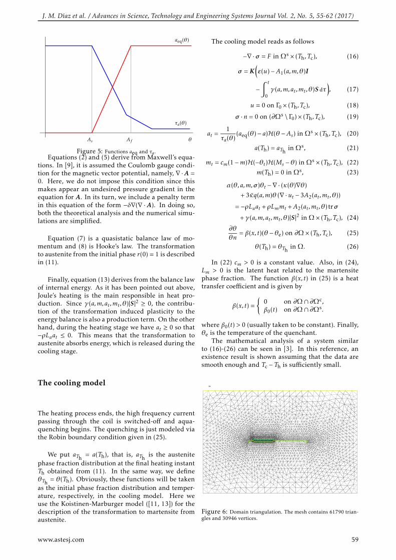
Dh

Figure 6: Domain triangulation. The mesh contains 61790 trian-gles and 30946 vertices.

www.astesj.com 59



3 Numerical simulation

Using the Freefem++ package ([8]), we have per-formed some numerical simulations for the approxi-mation of the solution to the systems (2)-(15) and (16)-(26). We want to describe the hardening treatment ofa car steering rack during the heating-cooling process.The goal is to produce martensite along the tooth linetogether with a thin layer in its neighborhood insidethe steel workpiece ([5, 6]).

Dh

Figure 7: Domain triangulation. Element density near threeteeth.

Figure 4 shows the open sets D, Ω = Ωs ∪Ωc ∪ Sand the faces Γ1 and Γ2 (they appear stick togetherin this figure) which intervene in the setting of theproblem. The workpiece contains a toothed part tobe hardened by means of the heating-cooling processdescribed above. It is made of a hypoeutectoid steel.The open set D \Ω is air. The magnetic permeability µin (5) is then given by

µ(x) =

µ0 if x ∈D \ Ω,0.99995µ0 if x ∈Ωc,2.24× 103µ0 if x ∈Ωs,

where µ0 = 4π × 10−7 (N/A2) is the magnetic constant(vacuum permeability).

The martensite phase can only derive from theaustenite phase. Thus we need to transform firstthe critical part to be hardened (the tooth line) intoaustenite. For our hypoeutectoid steel, austeniteonly exists in a temperature range close to the in-terval [1050,1670] (in K). During the first stage, theworkpiece is heated up by conduction and induction(Joule’s heating) which renders the tooth line up tothe desired temperature. In order to transform theaustenite into martensite, we must cool it down at avery high rate. This second stage is accomplished byaquaquenching.

In this simulation, the final time of the heatingprocess is Th = 5.5 seconds and the cooling processextends also for 5.5 seconds, that is Tc = 11.

We have used the finite elements method for thespace approximation and a Crank-Nicolson schemefor the time discretization. Figures 6 and 7 show thetriangulation of D in our numerical simulations. Wehave used P2-Lagrange approximation for ϕ, A and θand P1 for a and m.

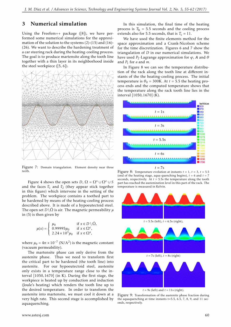
In Figure 8 we can see the temperature distribu-tion of the rack along the tooth line at different in-stants of the the heating-cooling process. The initialtemperature is θ0 = 300K. At t = 5.5 the heating pro-cess ends and the computed temperature shows thatthe temperature along the rack tooth line lies in theinterval [1050,1670] (K).

t = 1s

t = 3s

t = 5.5s

t = 6s

t = 7sFigure 8: Temperature evolution at instants t = 1, t = 3, t = 5.5(end of the heating stage, aqua-quenching begins), t = 6 and t = 7seconds, respectively. At t = 5.5s the temperature along the toothpart has reached the austenization level in this part of the rack. Thetemperature is measured in Kelvin.

t = 5.5s (left), t = 6.5s (right),

t = 7s (left), t = 8s (right)

t = 9s (left) and t = 11s (right).

Figure 9: Transformation of the austenite phase fraction duringthe aquaquenching at time instants t=5.5, 6.5, 7, 8, 9, and 11 sec-onds, respectively.

www.astesj.com 60



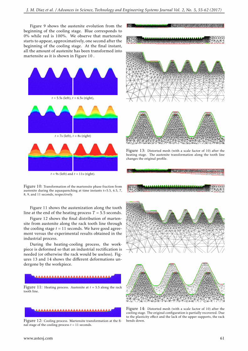
Figure 9 shows the austenite evolution from thebeginning of the cooling stage. Blue corresponds to0% while red is 100%. We observe that martensitestarts to appear, approximatively, one second after thebeginning of the cooling stage. At the final instant,all the amount of austenite has been transformed intomartensite as it is shown in Figure 10 .

t = 5.5s (left), t = 6.5s (right),

t = 7s (left), t = 8s (right)

t = 9s (left) and t = 11s (right).

Figure 10: Transformation of the martensite phase fraction fromaustenite during the aquaquenching at time instants t=5.5, 6.5, 7,8, 9, and 11 seconds, respectively.

Figure 11 shows the austenization along the toothline at the end of the heating process T = 5.5 seconds.

Figure 12 shows the final distribution of marten-site from austenite along the rack tooth line throughthe cooling stage t = 11 seconds. We have good agree-ment versus the experimental results obtained in theindustrial process.

During the heating-cooling process, the work-piece is deformed so that an industrial rectification isneeded (or otherwise the rack would be useless). Fig-ures 13 and 14 shows the different deformations un-dergone by the workpiece.

Figure 11: Heating process. Austenite at t = 5.5 along the racktooth line.

Figure 12: Cooling process. Martensite transformation at the fi-nal stage of the cooling process t = 11 seconds.

Figure 13: Distorted mesh (with a scale factor of 10) after theheating stage. The austenite transformation along the tooth linechanges the original profile.

Figure 14: Distorted mesh (with a scale factor of 10) after thecooling stage. The original configuration is partially recovered. Dueto the plasticity effect and the lack of the upper supports, the rackbends down.

www.astesj.com 61



Conflict of Interest The authors declare no conflictof interest.

Acknowledgments This research was partially sup-ported by Ministerio de Educacion y Ciencia undergrants MTM2010-16401 and TEC2014-54357-C2-2-R with the participation of FEDER, and Consejerıade Educacion y Ciencia de la Junta de Andalucıa, re-search group FQM–315.

References[1] A. Bermudez, J. Bullon, F. Pena and P. Salgado, “A numer-

ical method for transient simulation of metallurgical com-pound electrodes”, Finite Elem. Anal. Des., 39, 283–299, 2003.https://doi.org/10.1016/S0168-874X(02)00069-0

[2] A. Bermudez, D. Gomez, M. C. Muniz and P. Salgado, “Tran-sient numerical simulation of a thermoelectrical problem incylindrical induction heating furnaces”, Adv. Comput. Math.,26, 39–62, 2007. https://doi.org/10.1007/s10444-005-7470-9

[3] K. Chełminski, D. Homberg and D. Kern, “On a ther-momechanical model of phase transitions in steel”,Adv. Math. Sci. Appl., 18, 119–140, 2008.

[4] J. R. Davis et al. “ASM Handbook: Heat Treating”, vol. 4, ASMInternational, USA, 2007.

[5] J. M. Dıaz Moreno, C. Garcıa Vazquez, M. T. Gonzalez Mon-tesinos and F. Ortegon Gallego, “Numerical simulation ofa Induction-Conduction Model Arising in Steel Hardeningmodel arising in steel hardening”, Lecture Notes in Engineer-ing and Computer Science, World Congress on Engineering2009, Volume II, July 2009, 1251–1255.

[6] J. M. Dıaz Moreno, C. Garcıa Vazquez, M. T. Gonzalez Mon-tesinos, F. Ortegon Gallego and G. Viglialoro, “Mathematical

modeling of heat treatment for a steering rack including me-chanical effects”, J. Numer. Math. 20, no. 3-4, 215–231, 2012.https://doi.org/10.1515/jnum-2012-0011

[7] J. Fuhrmann, D. Homberg and M. Uhle, “Numerical simula-tion of induction hardening of steel”, COMPEL, 18, No. 3,482–493, 1999.https://doi.org/10.1108/03321649910275161

[8] F. Hecht, “New development in freeFem++”, J. Numer. Math.20, no. 3-4, 251–265, 2012. https://doi.org/10.1515/jnum-2012-0013

[9] D. Homberg, “A mathematical model for induction hard-ening including mechanical effects”, Nonlinear Anal.-RealWorld Appl., 5, 55–90, 2004. https://doi.org/10.1016/S1468-1218(03)00017-8

[10] D. Homberg and W. Weiss, “PID control of laser surface hard-ening of steel”, IEEE Trans. Control Syst. Technol., 14, No. 5,896–904, 2006. https://doi.org/10.1109/TCST.2006.879978

[11] D. P. Koistinen, R. E. Marburger, “A general equation pre-scribing the extent of the austenite-martensite transforma-tion in pure iron-carbon alloys and plain carbon steels”,Acta Metall., 7, 59–60, 1959. https://doi.org/10.1016/0001-6160(59)90170-1

[12] G. Krauss, “Steels: Heat Treatment and Processing Princi-ples”, ASM International, USA, 2000.

[13] J. B. Leblond and J. Devaux, “A new kinetic model foranisothermal metallurgical transformations in steels includ-ing effect of austenite grain size”, Acta Metall., 32, No. 1, 137–146, 1984. https://doi.org/10.1016/0001-6160(84)90211-6

[14] F. J. Pena Brage, “Contribucion al modelado matematico de al-gunos problemas en la metalurgia del silicio”, Ph. thesis, Uni-versidade de Santiago de Compostela, 2003.

[15] H. M. Yin, “Regularity of weak solution to Maxwell’s equa-tions and applications to microwave heating”, J. Differ. Equ.,200, 137-161, 2004.https://doi.org/10.1016/j.jde.2004.01.010

www.astesj.com 62


Documents

Steel heat treating: mathematical modelling and numerical