Embed Size (px)
Citation preview

A Math PrimerA review of basic quantitative skills
for theMPA Program in Environmental Science and Policy
Prepared by Dr. P. Louchouarn

Math Primer (MPA Environmental Sciences and Policy) i
Table of Contents1) Algebraic Expressions..................................................................................... 1
a. Simplifying Algebraic Expressions...................................................... 1b. Solutions of Algebraic Expressions...................................................... 2c. Addition Principle ............................................................................... 3d. Multiplication Principle ....................................................................... 4e. Using the Principles Together.............................................................. 5
2) Word Problems ............................................................................................... 6a. General Word Problems....................................................................... 6
3) Graphing and Straight Lines............................................................................ 8a. Rectangular Coordinates...................................................................... 8b. Graphing Functions ............................................................................. 9c. Straight Lines .................................................................................... 10
4) Systems of Linear Equations ......................................................................... 14a. The Solutions of a Systems of Equations ........................................... 14b. Addition Method ............................................................................... 15c. Substitution Method .......................................................................... 17
5) Exponents and Roots..................................................................................... 18a. Exponents.......................................................................................... 18b. Roots ................................................................................................. 19c. Simplifying Radical Expressions ....................................................... 20d. Rationalizing the Denominator .......................................................... 20
6) Quadratic Equations ...................................................................................... 22a. Definition .......................................................................................... 22b. Solving Quadratic Equations ............................................................. 22
i. Solving by Square Roots ........................................................ 22 ii. Solving by Factoring.............................................................. 22 iii. Solving by Completing the Squares........................................ 23 iv. Solving Using the Quadratic Formula .................................... 24
7) Basic Concepts of Statistics........................................................................... 26a. Introduction....................................................................................... 26b. Measurement ..................................................................................... 26c. Central Tendencies ............................................................................ 27
i. Mean...................................................................................... 28 ii. Median................................................................................... 28 iii. Mode ..................................................................................... 28
d. Correlations....................................................................................... 29 i. Calculation of Correlation Coefficient.................................... 31
e. Bivariate Linear Regression............................................................... 32 i. Introduction ........................................................................... 32 ii. Linear Regression Analysis.................................................... 33 iii. Interpretation ......................................................................... 34
8) Operations’ Reminder ................................................................................... 359) References .................................................................................................... 39

Math Primer (MPA Environmental Sciences and Policy) 1
Algebraic Expressions
Variablesÿ Letters represent an unknown or generic real
numberÿ Sometimes with restrictions, such as a member
of a certain set, or the set of values that makes anequation true.
ÿ Often a letter from the end of the alphabet: x, y, zÿ Or a letter that stands for a physical quantity: d
for distance, t for time, etc.
Constantsÿ Fixed values, like 2 or 7ÿ Can also be represented by letters: a, b, c, p, e, k
TermsTerms are Separated by + or –
FactorsFactors are multiplied together.
CoefficientsCoefficients are constant factors that multiply avariable or powers of a variable
The middle term has 2 factors, –3 and x. We say thatthe coefficient of x is –3.
The first term has three factors, 2 and two factors ofx. We say that 2 is the coefficient of x2.
The last term is a factor all by itself (although thenumber 4 could be factored into 2 x 2).
Simplifying Algebraic Expressions
By “simplifying” an algebraic expression, we meanwriting it in the most compact or efficient manner,without changing the value of the expression. Thismainly involves collecting like terms, which meansthat we add together anything that can be addedtogether. The rule here is that only like terms can beadded together.
Like (or similar) termsLike terms are those terms which contain the samepowers of same variables. They can have differentcoefficients, but that is the only difference.
Examples:
3x, x, and –2x are like terms.
2x2, –5x2, and are like terms.
xy2, 3y2 x, and 3xy2 are like terms.
xy2 and x2 y are NOT like terms, because the samevariable is not raised to the same power.
Combining Like termsCombining like terms is permitted because of thedistributive law. For example,
3x2 + 5x2 = (3 + 5)x2 = 8x2
What happened here is that the distributive law wasused in reverse—we “undistributed” a commonfactor of x2 from each term. The way to think aboutthis operation is that if you have three x-squareds,and then you get five more x-squareds, you will thenhave eight x-squareds.
Example: x2 + 2x + 3x2 + 2 + 4x + 7
Starting with the highest power of x, we see thatthere are four x-squareds in all (1x2 + 3x2). Then wecollect the first powers of x, and see that there are sixof them (2x + 4x). The only thing left is the constants2 + 7 = 9. Putting this all together we get
x2 + 2x + 3x2 + 2 + 4x + 7=
4x2 + 6x + 9
Math Primer (MPA Environmental Sciences and Policy) 2
Parentheses• Parentheses must be multiplied out before
collecting like termsYou cannot combine things in parentheses (or othergrouping symbols) with things outside theparentheses. Think of parentheses as opaque—thestuff inside the parentheses can’t “see” the stuffoutside the parentheses. If there is some factormultiplying the parentheses, then the only way to getrid of the parentheses is to multiply using thedistributive law.
Example: 3x + 2(x – 4) = 3x + 2x – 8
= 5x – 8
Minus Signs: Subtraction and Negatives
Subtraction can be replaced by adding the opposite3x – 2 = 3x + (–2)
Negative signs in front of parenthesesA special case is when a minus sign appears in frontof parentheses. At first glance, it looks as thoughthere is no factor multiplying the parentheses, andyou may be tempted to just remove the parentheses.What you need to remember is that the minus signindicating subtraction should always be thought of asadding the opposite. This means that you want to addthe opposite of the entire thing inside theparentheses, and so you have to change the sign ofeach term in the parentheses. Another way of lookingat it is to imagine an implied factor of one in front ofthe parentheses. Then the minus sign makes thatfactor into a negative one, which can be multipliedby the distributive law:
3x – (2 – x)
= 3x + (–1)[2 + (–x)]
= 3x + (–1)(2) + (–1)(–x)
= 3x – 2 + x
= 4x – 2
However, if there is only a plus sign in front of theparentheses, then you can simply erase theparentheses:
3x + (2 – x)
= 3x + 2 – x
A comment about subtraction and minus signsAlthough you can always explicitly replacesubtraction with adding the opposite, as in thisprevious example, it is often tedious andinconvenient to do so. Once you get used to thinkingthat way, it is no longer necessary to actually write itthat way. It is helpful to always think of minus signsas being “stuck” to the term directly to their right.That way, as you rearrange terms, collect like terms,and clear parentheses, the “adding the opposite”business will be taken care of because the minussigns will go with whatever was to their right. If whatis immediately to the right of a minus sign happensto be a parenthesis, and then the minus sign attacksevery term inside the parentheses.
Solutions of Algebraic Equations
Up until now, we have just been talking aboutmanipulating algebraic expressions. Now it is time totalk about equations. An expression is just astatement like
2x + 3
This expression might be equal to any number,depending on the choice of x. For example, if x = 3then the value of this expression is 9. But if we arewriting an equation, then we are making a statementabout its value. We might say
2x + 3 = 7
A mathematical equation is either true or false. Thisequation, 2x + 3 = 7, might be true or it might befalse; it depends on the value chosen for x. We callsuch equations conditional, because their truthdepends on choosing the correct value for x. If Ichoose x = 3, then the equation is clearly falsebecause 2(3) + 3 = 9, not 7. In fact, it is only true if Ichoose x = 2. Any other value for x produces a falseequation. We say that x = 2 is the solution of thisequation.
Solutionsÿ The solution of an equation is the value(s) of the
variable(s) that make the equation a truestatement.
An equation like 2x + 3 = 7 is a simple type called alinear equation in one variable. These will alwayshave one solution, no solutions, or an infinite numberof solutions. There are other types of equations,

Math Primer (MPA Environmental Sciences and Policy) 3
however, that can have several solutions. Forexample, the equation
x2 = 9
is satisfied by both 3 and –3, and so it has twosolutions.
One SolutionThis is the normal case, as in our example where theequation 2x + 3 = 7 had exactly one solution, namelyx = 2. The other two cases, no solution and an infinitenumber of solutions, are the oddball cases that youdon’t expect to run into very often. Nevertheless, it isimportant to know that they can happen in case youdo encounter one of these situations.
Infinite Number of SolutionsConsider the equation
x = x
This equation is obviously true for every possiblevalue of x. This is, of course, a ridiculously simpleexample, but it makes the point. Equations that havethis property are called identities. Some examples ofidentities would be
2x = x + x
3 = 3
(x – 2)(x + 2) = x2 – 4
All of these equations are true for any value of x.The second example, 3 = 3, is interesting because itdoes not even contain an x, so obviously itstruthfulness cannot depend on the value of x! Whenyou are attempting to solve an equation algebraicallyand you end up with an obvious identity (like 3 = 3),then you know that the original equation must also bean identity, and therefore it has an infinite number ofsolutions.
No SolutionsNow consider the equation
x + 4 = x + 3
There is no possible value for x that could make thistrue. If you take a number and add 4 to it, it willnever be the same as if you take the same numberand add 3 to it. Such an equation is called acontradiction, because it cannot ever be true.
If you are attempting to solve such an equation, youwill end up with an extremely obvious contradiction
such as 1 = 2. This indicates that the originalequation is a contradiction, and has no solution.
In summary,
ÿ An identity is always true, no matter what x isÿ A contradiction is never true for any value of xÿ A conditional equation is true for some values of
x
Addition Principle
Equivalent EquationsThe basic approach to finding the solution toequations is to change the equation into simplerequations, but in such a way that the solution set ofthe new equation is the same as the solution set of theoriginal equation. When two equations have the samesolution set, we say that they are equivalent.
What we want to do when we solve an equation is toproduce an equivalent equation that tells us thesolution directly. Going back to our previousexample,
2x + 3 = 7
we can say that the equation
x = 2
is an equivalent equation, because they both have thesame solution, namely x = 2. We need to have someway to convert an equation like 2x + 3 = 7 into anequivalent equation like x = 2 that tells us thesolution. We solve equations by using methods thatrearrange the equation in a manner that does notchange the solution set, with a goal of getting thevariable by itself on one side of the equal sign. Thenthe solution is just the number that appears on theother side of the equal sign.
The methods of changing an equation withoutchanging its solution set are based on the idea that ifyou change both sides of an equation in the sameway, then the equality is preserved. Think of anequation as a balance—whatever complicatedexpression might appear on either side of theequation, they are really just numbers. The equal signis just saying that the value of the expression on theleft side is the same number as the value on the rightside. Therefore, no matter how horrible the equationmay seem, it is really just saying something like3 = 3.

Math Primer (MPA Environmental Sciences and Policy) 4
The Addition PrincipleAdding (or subtracting) the same number to bothsides of an equation does not change its solution set.
Think of the balance analogy—if both sides of theequation are equal, then increasing both sides by thesame amount will change the value of each side, butthey will still be equal. For example, if
3 = 3,
then
3 + 2 = 3 + 2.
Consequently, if
6 + x = 8
for some value of x (which in this case is x = 2), thenwe can add any number to both sides of the equationand x = 2 will still be the solution. If we wanted to,we could add a 3 to both sides of the equation,producing the equation
9 + x = 11.
As you can see, x = 2 is still the solution. Of course,this new equation is no simpler than the one westarted with, and this maneuver did not help us solvethe equation.If we want to solve the equation
6 + x = 8,
the idea is to get x by itself on one side, and so wewant to get rid of the 6 that is on the left side. We cando this by subtracting a 6 from both sides of theequation (which of course can be thought of asadding a negative six):
6 – 6 + x = 8 – 6
or
x = 2
You can think of this operation as moving the 6from one side of the equation to the other, whichcauses it to change sign The addition principle is useful in solving equationsbecause it allows us to move whole terms from oneside of the equal sign to the other. While this is aconvenient way to think of it, you should rememberthat you are not really “moving” the term from oneside to the other—you are really adding (orsubtracting) the term on both sides of the equation.
NotationsIn the previous example, we wrote the –6 in-line withthe rest of the equation. This is analogous to writingan arithmetic subtraction problem in one line, as in
234 – 56 = 178.
You probably also learned to write subtraction andaddition problems in a column format, like
We can also use a similar notation for the additionmethod with algebraic equations.Given the equation
x + 3 = 2,
we want to subtract a 3 from both sides in order toisolate the variable. In column format this wouldlook like
Here the numbers in the second row are negative 3’s,so we are adding the two rows together to producethe bottom row.
The advantage of the column notation is that it makesthe operation easier to see and reduces the chancesfor an error. The disadvantage is that it takes morespace, but that is a relatively minor disadvantage.Which notation you prefer to use is not important, aslong as you can follow what you are doing and itmakes sense to you.
Multiplication Principle
Multiplying (or dividing) the same non-zero numberto both sides of an equation does not change itssolution set.
Example:
so if 6x = 12, then 18x = 36 for the same value of x(which in this case is x = 2).
The way we use the multiplication principle to solveequations is that it allows us to isolate the variable bygetting rid of a factor that is multiplying the variable.

Math Primer (MPA Environmental Sciences and Policy) 5
Example: 2x = 6
To get rid of the 2 that is multiplying the x, we candivide both sides of the equation by 2, or multiply byits reciprocal (one-half).Either divide both sides by 2:
or multiply both sides by a half:
• Whether you prefer to think of it as dividing bythe number or multiplying by its reciprocal is notimportant, although when the coefficient is afraction it is easier to multiply by the reciprocal:
Example: 4/5x = 8
Multiply both sides by the reciprocal of thecoefficient, or 5/4
Using the Principles Together
Suppose you were given an equation like
2x – 3 = 5. You will need to use the addition principle to movethe –3, and the multiplication principle to remove thecoefficient 2. Which one should you use first?Strictly speaking, it does not matter—you willeventually get the right answer. In practice, however,it is usually simpler to use the addition principle first,and then the multiplication principle. The reason forthis is that if we divide by 2 first we will turneverything into fractions:
Given: 2x – 3 = 5
Suppose we first divide both sides by 2:
Now there is nothing wrong with doing arithmeticwith fractions, but it is not as simple as working withwhole numbers. In this example we would have toadd 3/2 to both sides of the equation to isolate the x.It is usually more convenient, though, to use theaddition principle first:
Given: 2x – 3 = 5
Add 3 to both sides:
At this point all we need to do is divide both sidesby 2 to get x = 4.

Math Primer (MPA Environmental Sciences and Policy) 6
Word Problems
Problem Solving Strategies
Understand1. Read the problem carefully.2. Make sure you understand the situation that is
described.3. Make sure you understand what information is
provided, and what the question is asking.4. For many problems, drawing a clearly labeled
picture is very helpful.
Plan1. First focus on the objective. What do you need to
know in order to answer the question?2. Then look at the given information. How can you
use that information to get what you need toknow to answer the question?
3. If you do not see a clear logical path leadingfrom the given information to the solution, justtry something. Look at the given information andthink about what you can find from it, even if itis not what the question is asking for. Often youwill find another piece of information that youcan then use to answer the question.
Write equationsYou need to express mathematically the logicalconnections between the given information and theanswer you are seeking. This involves:
1. Assigning variable names to the unknownquantities. The letter x is always popular, but it isa good idea to use something that reminds youwhat it represents, such as d for distance or t fortime. The trickiest part of assigning variables isthat you want to use a minimum number ofdifferent variables (just one if possible). If youknow how two quantities are related, then youcan express them both with just one variable. Forexample, if Jim is two years older than John is,you might let x stand for John’s age and (x + 2)stand for Jim’s age.
2. Translate English into Math. Mathematics is alanguage, one that is particularly well suited todescribing logical relationships. English, on theother hand, is much less precise.
SolveNow you just have to solve the equation(s) for theunknown(s). Remember to answer the question thatthe problem asks.
Check!Think about your answer. Does your answer comeout in the correct units? Is it reasonable? If you madea mistake somewhere, chances are your answer willnot just be a little bit off, but will be completelyridiculous
General Word Problems
General StrategyRecall the general strategy for setting up wordproblems. Refer to the Problem Solving Strategiespage for more detail.1. Read the problem carefully: Determine what is
known, what is unknown, and what question isbeing asked.
2. Represent unknown quantities in terms of avariable.
3. Use diagrams where appropriate.4. Find formulas or mathematical relationships
between the knowns and the unknowns.5. Solve the equations for the unknowns.6. Check answers to see if they are reasonable.
Number ProblemsExample: Find a number such that 5 more than one-half the number is three times the number.Let x be the unknown number.
Translating into math: 5 + x/2 = 3x
Solving:(First multiply by 2 to clear the fraction)
5 + x/2 = 3x
10 + x = 6x
10 = 5x
x = 2
Geometry ProblemsExample: If the perimeter of a rectangle is 10inches, and one side is one inch longer than the other,how long are the sides?

Math Primer (MPA Environmental Sciences and Policy) 7
Let one side be x and the other side be x + 1.
Then the given condition may be expressed as
x + x + (x + 1) + (x + 1) = 10
Solving:4x + 2 = 10
4x = 8x = 2
so the sides have length 2 and 3.
Rate-Time Problems
Rate = Quantity/Time
or
Quantity = Rate x Time
Example 1: A fast employee can assemble 7 radiosin an hour, and another slower employee can onlyassemble 5 radios per hour. If both employees worktogether, how long will it take to assemble 26 radios?
The two together will build 7 + 5 = 12 radios in anhour, so their combined rate is 12 radios/hr.
Using Time = Quantity/Rate, Time = 26/12 = 2 1/6 h
or
2 hours 10 minutes
Example 2: you are driving along at 55 mph whenyou are passed by a car doing 85 mph. How long willit take for the car that passed you to be one mileahead of you?
We know the two rates, and we know that thedifference between the two distances traveled will beone mile, but we don’t know the actual distances. LetD be the distance that you travel in time t, and D + 1be the distance that the other car traveled in time t.
Using the rate equation in the formdistance = speed • time for each car we can write
D = 55 t, and D + 1 = 85 t
Substituting the first equation into the second,
55t + 1 = 85t
-30t = -1
t = 1/30 hr(or 2 minutes)
Mixture ProblemsExample: How much of a 10% vinegar solutionshould be added to 2 cups of a 30% vinegar solutionto make a 20% solution?
Let x be the unknown volume of 10% solution. Writean equation for the volume of vinegar in eachmixture:
(amount of vinegar in first solution) + (amount ofvinegar in second solution) = (amount of vinegar intotal solution)
0.1x + 0.3(2) = 0.2(x + 2)
0.1x + 0.6 = 0.2x + 0.4
-0.1x = -0.2
x = 2 cups

Math Primer (MPA Environmental Sciences and Policy) 8
Graphing and straight Lines
A. Rectangular Coordinates
The rectangular coordinate system is also known asthe Cartesian coordinate system after ReneDescartes, who popularized its use in analyticgeometry. The rectangular coordinate system isbased on a grid, and every point on the plane can beidentified by unique x and y coordinates, just as anypoint on the Earth can be identified by giving itslatitude and longitude.
AxesLocations on the grid are measured relative to a fixedpoint, called the origin, and are measured accordingto the distance along a pair of axes. The x and y axesare just like the number line, with positive distancesto the right and negative to the left in the case of the
x axis, and positive distances measured upwards andnegative down for the y axis. Any displacement awayfrom the origin can be constructed by moving aspecified distance in the x direction and then anotherdistance in the y direction. Think of it as if you weregiving directions to someone by saying somethinglike “go three blocks East and then 2 blocks North.”
Coordinates, Graphing Points
We specify the location of a point by first giving its xcoordinate (the left or right displacement from theorigin), and then the y coordinate (the up or downdisplacement from the origin). Thus, every point onthe plane can be identified by a pair of numbers(x, y), called its coordinates.
Examples:

Math Primer (MPA Environmental Sciences and Policy) 9
QuadrantsSometimes we just want to know what general partof the graph we are talking about. The axes naturallydivide the plane up into quarters. We call thesequadrants, and number them from one to four.Notice that the numbering begins in the upper rightquadrant and continues around in the counter-clockwise direction. Notice also that each quadrantcan be identified by the unique combination ofpositive and negative signs for the coordinates of apoint in that quadrant.
B. Graphing Functions
Consider an equation such as
y = 2x – 1
We say that y is a function of x because if you chooseany value for x, this formula will give you a uniquevalue of y. For example, if we choose x = 3 then theformula gives us
y = 2(3) – 1
or
y = 5
Thus we can say that the value y = 5 is generated bythe choice of x = 3. Had we chosen a different valuefor x, we would have gotten a different value for y. Infact, we can choose a whole bunch of differentvalues for x and get a y value for each one. This isbest shown in a table:
x (input) x – Formula - y y (output)–2 2(–2) – 1 = –5 –5–1 2(–1) – 1 = –3 –30 2(0) – 1 = –1 –11 2(1) – 1 = 1 12 2(2) – 1 = 3 33 2(3) – 1 = 5 5
This relationship between x and its corresponding yvalues, produces a collection of pairs of points (x, y),namely
(–2, –5)(–1, –3)(0, –1)(1, 1)(2, 3)(3, 5)
Since each of these pairs of numbers can be thecoordinates of a point on the plane, it is natural to askwhat this collection of ordered pairs would look likeif we graphed them. The result is something like this:
The points seem to fall in a straight line. Now, ourchoices for x were quite arbitrary. We could just aswell have picked other values, including non-integervalues. Suppose we picked many more values for x,like 2.7, 3.14, etc. and added them to our graph.Eventually the points would be so crowded togetherthat they would form a solid line:
The arrows on the ends of the line indicate that itgoes on forever, because there is no limit to whatnumbers we could choose for x. We say that this lineis the graph of the function y = 2x – 1.
If you pick any point on this line and read off its xand y coordinates, they will satisfy the equation

Math Primer (MPA Environmental Sciences and Policy) 10
y = 2x – 1. For example, the point (1.5, 2) is on theline:
and the coordinates x = 1.5, y = 2 satisfy the equationy = 2x – 1:
2 = 2(1.5) – 1
Note: This graph turned out to be a straight line onlybecause of the particular function that we used as anexample. There are many other functions whosegraphs turn out to be various curves.
C. Straight Lines
Linear Equations in Two VariablesThe equation y = 2x – 1 that we used as an examplefor graphing functions produced a graph that was astraight line. This was no accident. This equation isone example of a general class of equations that wecall linear equations in two variables. The twovariables are usually (but of course don’t have to be)x and y. The equations are called linear because theirgraphs are straight lines. Linear equations are easy torecognize because they obey the following rules:
1. The variables (usually x and y) appear only to thefirst power
2. The variables may be multiplied only by realnumber constants
3. Any real number term may be added (orsubtracted, of course)
4. Nothing else is permitted!
* This means that any equation containing things likex2, y2, 1/x, xy, square roots, or any other function of xor y is not linear.
Describing LinesJust as there are an infinite number of equations thatsatisfy the above conditions, there are also an infinitenumber of straight lines that we can draw on a graph.To describe a particular line we need to specify two
distinct pieces of information concerning that line. Aspecific straight line can be determined by specifyingtwo distinct points that the line passes through, or itcan be determined by giving one point that it passesthrough and somehow describing how “tilted” theline is.
SlopeThe slope of a line is a measure of how “tilted” theline is. A highway sign might say something like“6% grade ahead.” What does this mean, other thanthat you hope your brakes work? What it means isthat the ratio of your drop in altitude to yourhorizontal distance is 6%, or 6/100. In other words, ifyou move 100 feet forward, you will drop 6 feet; ifyou move 200 feet forward, you will drop 12 feet,and so on.
We measure the slope of lines in much the same way,although we do not convert the result to a percent.
Suppose we have a graph of an unknown straightline. Pick any two different points on the line andlabel them point 1 and point 2:
In moving from point 1 to point 2, we cover 4 stepshorizontally (the x direction) and 2 steps vertically(the y direction):
Therefore, the ratio of the change in altitude to thechange in horizontal distance is 2 to 4. Expressing it

Math Primer (MPA Environmental Sciences and Policy) 11
as a fraction and reducing, we say that the slope ofthis line is
To formalize this procedure a bit, we need to thinkabout the two points in terms of their x and ycoordinates.
Now you should be able to see that the horizontaldisplacement is the difference between the xcoordinates of the two points, or
4 = 5 – 1,
and the vertical displacement is the differencebetween the y coordinates, or
2 = 4 – 2.
In general, if we say that the coordinates of point 1are (x1, y1) and the coordinates of point 2 are(x2, y2),
then we can define the slope m as follows:
where (x1, y1) and (x2, y2) are any two distinctpoints on the line.
ÿ It is customary (in the US) to use the letter m torepresent slope. No one knows why.
ÿ It makes no difference which two points are usedfor point 1 and point 2. If they were switched,
both the numerator and the denominator of thefraction would be changed to the opposite sign,giving exactly the same result.
ÿ Many people find it useful to remember thisformula as “slope is rise over run.”
ÿ Another common notation is m = Dy/Dx, wherethe Greek letter delta (D) means “the change in.”The slope is a ratio of how much y changes perchange in x:
Horizontal Lines
A horizontal line has zero slope, because there is nochange in y as x increases. Thus, any two points willhave the same y coordinates, and since y1 = y2,
Vertical Lines
A vertical line presents a different problem. If youlook at the formula

Math Primer (MPA Environmental Sciences and Policy) 12
you see that there is a problem with the denominator.It is not possible to get two different values for xl andx2, because if x changes then you are not on thevertical line anymore. Any two points on a verticalline will have the same x coordinates, and sox2 – x1 = 0. Since the denominator of a fractioncannot be zero, we have to say that a vertical linehas undefined slope. Do not confuse this with thecase of the horizontal line, which has a well-definedslope that just happens to equal zero.
Positive and Negative SlopeThe x coordinate increases to the right, so movingfrom left to right is motion in the positive x direction.Suppose that you are going uphill as you move in thepositive x direction. Then both your x and ycoordinates are increasing, so the ratio of rise overrun will be positive—you will have a positiveincrease in y for a positive increase in x. On the otherhand, if you are going downhill as you move fromleft to right, then the ratio of rise over run will benegative because you lose height for a given positiveincrease in x. The thing to remember is:As you go from left to right,
ÿ Uphill = Positive Slopeÿ Downhill = Negative Slope
And of course, no change in height means that theline has zero slope.
Some Slopes
InterceptsTwo lines can have the same slope and be indifferent places on the graph. This means that inaddition to describing the slope of a line we needsome way to specify exactly where the line is on thegraph. This can be accomplished by specifying oneparticular point that the line passes through.Although any point will do, it is conventional to
specify the point where the line crosses the y-axis.This point is called the y-intercept, and is usuallydenoted by the letter b. Note that every line exceptvertical lines will cross the y-axis at some point, andwe have to handle vertical lines as a special caseanyway because we cannot define a slope for them.
Same Slopes, Different y-Intercepts
EquationsThe equation of a line gives the mathematicalrelationship between the x and y coordinates of anypoint on the line.
Let’s return to the example we used in graphingfunctions. The equation
y = 2x – 1
produces the following graph:
This line evidently has a slope of 2 and a y interceptequal to –1. The numbers 2 and –1 also appear in theequation—the coefficient of x is 2, and the additiveconstant is –1. This is not a coincidence, but is due tothe standard form in which the equation was written.

Math Primer (MPA Environmental Sciences and Policy) 13
Standard Form (Slope-Intercept Form)If a linear equation in two unknowns is written in theform
y = mx + b
where m and b are any two real numbers, then thegraph will be a straight line with a slope of m and a yintercept equal to b.
Point-Slope Form
As mentioned earlier, a line is fully described bygiving its slope and one distinct point that the linepasses through. While this point is customarily the yintercept, it does not need to be. If you want todescribe a line with a given slope m that passesthrough a given point (x1, y1), the formula is
To help remember this formula, think of solving itfor m:
Since the point (x, y) is an arbitrary point on the lineand the point (x1, y1) is another point on the line, thisis nothing more than the definition of slope for thatline.
Two-Point FormAnother way to completely specify a line is to givetwo different points that the line passes through. Ifyou are given that the line passes through the points(x1, y1) and (x2, y2), the formula is
This formula is also easy to remember if you noticethat it is just the same as the point-slope form withthe slope m replaced by the definition of slope,

Math Primer (MPA Environmental Sciences and Policy) 14
Systems of Linear Equations
A. The Solutions of a System of Equations
A system of equations refers to a number ofequations with an equal number of variables. We willonly look at the case of two linear equations in twounknowns. The situation gets much more complex asthe number of unknowns increases, and largersystems are commonly attacked with the aid of acomputer.
A system of two linear equations in two unknownsmight look like
This is the standard form for writing equations whenthey are part of a system of equations: the variablesgo in order on the left side and the constant term ison the right. The bracket on the left indicates that thetwo equations are intended to be solvedsimultaneously, but it is not always used.
When we talk about the solution of this system ofequations, we mean the values of the variables thatmake both equations true at the same time. Theremay be many pairs of x and y that make the firstequation true, and many pairs of x and y that makethe second equation true, but we are looking for an xand y that would work in both equations. In thefollowing pages we will look at algebraic methodsfor finding this solution, if it exists.
Because these are linear equations, their graphs willbe straight lines. This can help us visualize thesituation graphically. There are three possibilities:
1. Independent Equationsÿ Lines intersectÿ One solution
In this case the two equations describe lines thatintersect at one particular point. Clearly this point ison both lines, and therefore its coordinates (x, y) willsatisfy the equation of either line. Thus the pair (x, y)is the one and only solution to the system ofequations.
2. Dependent Equationsÿ Equations describe the same lineÿ Infinite number of solutions
Sometimes two equations might look different butactually describe the same line. For example, in
The second equation is just two times the firstequation, so they are actually equivalent and wouldboth be equations of the same line. Because the twoequations describe the same line, they have all theirpoints in common; hence there are an infinite numberof solutions to the system.
ÿ Attempting to solve gives an identityIf you try to solve a dependent system by algebraicmethods, you will eventually run into an equationthat is an identity. An identity is an equation that isalways true, independent of the value(s) of anyvariable(s). For example, you might get an equationthat looks like x = x, or 3 = 3. This would tell youthat the system is a dependent system, and you couldstop right there because you will never find a uniquesolution.

Math Primer (MPA Environmental Sciences and Policy) 15
3. Inconsistent Equationsÿ Lines do not intersect (Parallel Lines; have the
same slope)ÿ No solutions
If two lines happen to have the same slope, but arenot identically the same line, then they will neverintersect. There is no pair (x, y) that could satisfyboth equations, because there is no point (x, y) that issimultaneously on both lines. Thus these equationsare said to be inconsistent, and there is no solution.The fact that they both have the same slope may notbe obvious from the equations, because they are notwritten in one of the standard forms for straight lines.The slope is not readily evident in the form we usefor writing systems of equations. (If you think aboutit you will see that the slope is the negative of thecoefficient of x divided by the coefficient of y).
• Attempting to solve gives a false statementBy attempting to solve such a system of equationsalgebraically, you are operating on a falseassumption—namely that a solution exists. This willeventually lead you to a contradiction: a statementthat is obviously false, regardless of the value(s) ofthe variable(s). At some point in your work youwould get an obviously false equation like 3!=!4.This would tell you that the system of equations isinconsistent, and there is no solution.!
Solution by GraphingFor more complex systems, and especially those thatcontain non-linear equations, finding a solution byalgebraic methods can be very difficult or evenimpossible. Using a graphing calculator (or acomputer), you can graph the equations and actuallysee where they intersect. The calculator can then giveyou the coordinates of the intersection point. Theonly drawback to this method is that the solution isonly an approximation, whereas the algebraic methodgives the exact solution. In most practical situations,though, the precision of the calculator is sufficient.For more demanding scientific and engineering
applications there are computer methods that can findapproximate solutions to very high precision.
B. Addition Method
The whole problem with solving a system ofequations is that you cannot solve an equation thathas two unknowns in it. You need an equation withonly one variable so that you can isolate the variableon one side of the equation. Both methods that wewill look at are techniques for eliminating one of thevariables to give you an equation in just oneunknown, which you can then solve by the usualmethods.
The first method of solving systems of linearequations is the addition method, in which the twoequations are added together to eliminate one of thevariables.
Adding the equations means that we add the leftsides of the two equations together, and we add theright sides together. This is legal because of theAddition Principle, which says that we can add thesame amount to both sides of an equation. Since theleft and right sides of any equation are equal to eachother, we are indeed adding the same amount to bothsides of an equation.
Consider this simple example:
Example:
If we add these equations together, the termscontaining y will add up to zero (2y plus -2y), and wewill get
or
5x = 5
x = 1
However, we are not finished yet—we know x, butwe still don’t know y. We can solve for y bysubstituting the now known value for x into either ofour original equations. This will produce an equationthat can be solved for y:

Math Primer (MPA Environmental Sciences and Policy) 16
Now that we know both x and y, we can say that thesolution to the system is the pair (1, 1/2).
This last example was easy to see because of thefortunate presence of both a positive and a negative2y. One is not always this lucky. Consider
Example:
Now there is nothing so obvious, but there is stillsomething we can do. If we multiply the firstequation by -3, we get
(Don’t forget to multiply every term in the equation,on both sides of the equal sign). Now if we add themtogether the terms containing x will cancel:
or
As in the previous example, now that we know y wecan solve for x by substituting into either originalequation. The first equation looks like the easiest tosolve for x, so we will use it:
And so the solution point is (-4, 7/2).
Now we look at an even less obvious example:
Example:
Here there is nothing particularly attractive aboutgoing after either the x or the y. In either case, bothequations will have to be multiplied by some factorto arrive at a common coefficient. This is very muchlike the situation you face trying to find a leastcommon denominator for adding fractions, exceptthat here we call it a Least Common Multiple(LCM). As a general rule, it is easiest to eliminatethe variable with the smallest LCM. In this case thatwould be the y, because the LCM of 2 and 3 is 6. Ifwe wanted to eliminate the x we would have to usean LCM of 10 (5 times 2). So, we choose to make thecoefficients of y into plus and minus 6. To do this,the first equation must be multiplied by 3, and thesecond equation by 2:
or
Now adding these two together will eliminate theterms containing y:
or
x = 2
We still need to substitute this value into one of theoriginal equation to solve for y:
Thus the solution is the point (2, 2).
Math Primer (MPA Environmental Sciences and Policy) 17
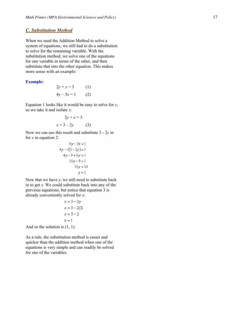
C. Substitution Method
When we used the Addition Method to solve asystem of equations, we still had to do a substitutionto solve for the remaining variable. With thesubstitution method, we solve one of the equationsfor one variable in terms of the other, and thensubstitute that into the other equation. This makesmore sense with an example:
Example:2y + x = 3 (1)
4y – 3x = 1 (2)
Equation 1 looks like it would be easy to solve for x,so we take it and isolate x:
2y + x = 3
x = 3 – 2y (3)
Now we can use this result and substitute 3 - 2y infor x in equation 2:
Now that we have y, we still need to substitute backin to get x. We could substitute back into any of theprevious equations, but notice that equation 3 isalready conveniently solved for x:
And so the solution is (1, 1).
As a rule, the substitution method is easier andquicker than the addition method when one of theequations is very simple and can readily be solvedfor one of the variables.
Math Primer (MPA Environmental Sciences and Policy) 18
Exponents and Roots
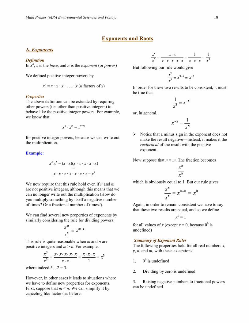
A. Exponents
DefinitionIn xn, x is the base, and n is the exponent (or power)
We defined positive integer powers by
xn = x · x · x · . . . · x (n factors of x)
PropertiesThe above definition can be extended by requiringother powers (i.e. other than positive integers) tobehave like the positive integer powers. For example,we know that
xn · xm = xn+m
for positive integer powers, because we can write outthe multiplication.
Example:
x2 x5 = (x · x)(x · x · x · x · x)=
x · x · x · x · x · x · x = x7
We now require that this rule hold even if n and mare not positive integers, although this means that wecan no longer write out the multiplication (How doyou multiply something by itself a negative numberof times? Or a fractional number of times?).
We can find several new properties of exponents bysimilarly considering the rule for dividing powers:
This rule is quite reasonable when m and n arepositive integers and m > n. For example:
where indeed 5 – 2 = 3.
However, in other cases it leads to situations wherewe have to define new properties for exponents.First, suppose that m < n. We can simplify it bycanceling like factors as before:
But following our rule would give
In order for these two results to be consistent, it mustbe true that
or, in general,
ÿ Notice that a minus sign in the exponent does notmake the result negative—instead, it makes it thereciprocal of the result with the positiveexponent.
Now suppose that n = m. The fraction becomes
which is obviously equal to 1. But our rule gives
Again, in order to remain consistent we have to saythat these two results are equal, and so we define
x0 = 1
for all values of x (except x = 0, because 00 isundefined)
Summary of Exponent RulesThe following properties hold for all real numbers x,y, n, and m, with these exceptions:
1. 00 is undefined
2. Dividing by zero is undefined
3. Raising negative numbers to fractional powerscan be undefined

Math Primer (MPA Environmental Sciences and Policy) 19
x1 = x
x0 = 1
xn · xm = xn+m
(xn)m = xnm
B. Roots
DefinitionRoots are the inverse of exponents. An nth root“undoes” raising a number to the nth power, andvice-versa. (The correct terminology for these typesof relationships is inverse functions, but powers androots can only be strictly classified as inversefunctions if we take care of some ambiguitiesassociated with plus or minus signs, so we will notworry about this yet). The common example is thesquare root, which “undoes” the act of squaring. Forexample, take 3 and square it to get 9. Now take thesquare root of 9 and get 3 again. It is also possible tohave roots related to powers other than the square.The cube root, for example, is the inverse of raisingto the power of 3. The cube root of 8 is 2 because 23
= 8. In general, the nth root of a number is written:
if and only if
because 43 = 64
We leave the index off the square root symbol onlybecause it is the most common one. It is understoodthat if no index is shown, then the index is 2.
if and only if
because 42 = 16
Square RootsThe square root is the inverse function of squaring(strictly speaking only for positive numbers, becausesign information can be lost)
Principal Rootÿ Every positive number has two square roots, one
positive and one negative
Example: 2 is a square root of 4 because 2 x 2 = 4,but –2 is also a square root of 4 because (–2) x(–2) = 4
To avoid confusion between the two we define thesymbol (this symbol is called a radical) to mean
the principal or positive square root.
The convention is: For any positive number x,
is the positive root, and
is the negative root.
If you mean the negative root, use a minus sign infront of the radical.
Example:
Properties
for all non-negative numbers x
for all non-negative numbers x
However, if x happens to be negative, then squaringit will produce a positive number, which will have apositive square root, so
for all real numbers x
ÿ You don’t need the absolute value sign if youalready know that x is positive. For example,
, and saying anything about the absolutevalue of 2 would be superfluous. You only needthe absolute value signs when you are taking thesquare root of a square of a variable, which maybe positive or negative.
ÿ The square root of a negative number isundefined, because anything times itself willgive a positive (or zero) result.
(your calculator will probablysay ERROR).
ÿ Note: Zero has only one square root (itself). Zerois considered neither positive nor negative.
WARNING: Do not attempt to do something likethe distributive law with radicals:
(WRONG) or
(WRONG).
Math Primer (MPA Environmental Sciences and Policy) 20
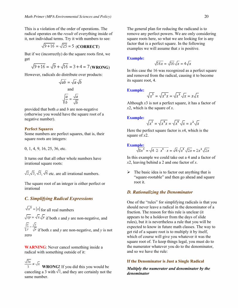
This is a violation of the order of operations. Theradical operates on the result of everything inside ofit, not individual terms. Try it with numbers to see:
(CORRECT)
But if we (incorrectly) do the square roots first, weget
(WRONG)
However, radicals do distribute over products:
and
provided that both a and b are non-negative(otherwise you would have the square root of anegative number).
Perfect SquaresSome numbers are perfect squares, that is, theirsquare roots are integers:
0, 1, 4, 9, 16, 25, 36, etc.
It turns out that all other whole numbers haveirrational square roots:
, , , etc. are all irrational numbers.
The square root of an integer is either perfect orirrational
C. Simplifying Radical Expressions
for all real numbers
if both x and y are non-negative, and
if both x and y are non-negative, and y is notzero
WARNING: Never cancel something inside aradical with something outside of it:
WRONG! If you did this you would becanceling a 3 with , and they are certainly not thesame number.
The general plan for reducing the radicand is toremove any perfect powers. We are only consideringsquare roots here, so what we are looking for is anyfactor that is a perfect square. In the followingexamples we will assume that x is positive.
Example:
In this case the 16 was recognized as a perfect squareand removed from the radical, causing it to becomeits square root, 4.
Example:
Although x3 is not a perfect square, it has a factor ofx2, which is the square of x.
Example:
Here the perfect square factor is x4, which is thesquare of x2.
Example:
In this example we could take out a 4 and a factor ofx2, leaving behind a 2 and one factor of x.
ÿ The basic idea is to factor out anything that is“square-rootable” and then go ahead and squareroot it.
D. Rationalizing the Denominator
One of the “rules” for simplifying radicals is that youshould never leave a radical in the denominator of afraction. The reason for this rule is unclear (itappears to be a holdover from the days of sliderules), but it is nevertheless a rule that you will beexpected to know in future math classes. The way toget rid of a square root is to multiply it by itself,which of course will give you whatever it was thesquare root of. To keep things legal, you must do tothe numerator whatever you do to the denominator,and so we have the rule:
If the Denominator is Just a Single Radical
Multiply the numerator and denominator by thedenominator
Math Primer (MPA Environmental Sciences and Policy) 21
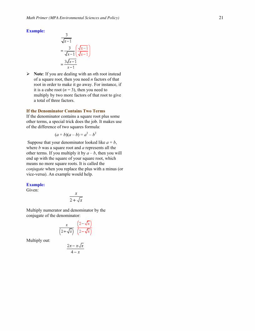
Example:
ÿ Note: If you are dealing with an nth root insteadof a square root, then you need n factors of thatroot in order to make it go away. For instance, ifit is a cube root (n = 3), then you need tomultiply by two more factors of that root to givea total of three factors.
If the Denominator Contains Two TermsIf the denominator contains a square root plus someother terms, a special trick does the job. It makes useof the difference of two squares formula:
(a + b)(a – b) = a2 – b2
Suppose that your denominator looked like a + b,where b was a square root and a represents all theother terms. If you multiply it by a – b, then you willend up with the square of your square root, whichmeans no more square roots. It is called theconjugate when you replace the plus with a minus (orvice-versa). An example would help. Example: Given:
Multiply numerator and denominator by theconjugate of the denominator:
Multiply out:
Math Primer (MPA Environmental Sciences and Policy) 22
Quadratic Equations
Definition
ax2 + bx + c = 0
a, b, c are constants (generally integers)
RootsSynonyms: Solutions or Zeros
ÿ Can have 0, 1, or 2 real roots
Consider the graph of quadratic equations. Thequadratic equation looks like ax2 + bx + c = 0, but ifwe take the quadratic expression on the left and setit equal to y, we will have a function:
y = ax2 + bx + c
When we graph y vs. x, we find that we get a curvecalled a parabola. The specific values of a, b, and ccontrol where the curve is relative to the origin (left,right, up, or down), and how rapidly it spreads out.Also, if a is negative then the parabola will beupside-down. What does this have to do withfinding the solutions to our original quadraticequation? Well, whenever y = 0 then the equationy = ax2 + bx + c is the same as our original equation.
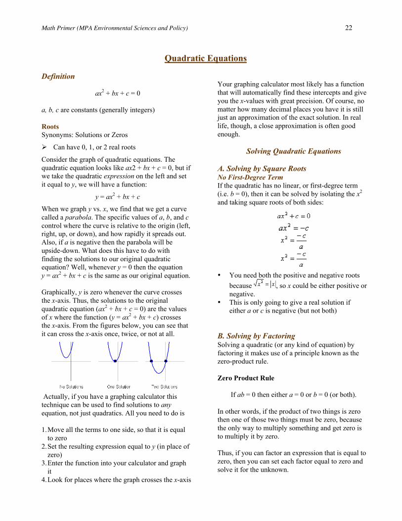
Graphically, y is zero whenever the curve crossesthe x-axis. Thus, the solutions to the originalquadratic equation (ax2 + bx + c = 0) are the valuesof x where the function (y = ax2 + bx + c) crossesthe x-axis. From the figures below, you can see thatit can cross the x-axis once, twice, or not at all.
Actually, if you have a graphing calculator thistechnique can be used to find solutions to anyequation, not just quadratics. All you need to do is 1. Move all the terms to one side, so that it is equal
to zero2. Set the resulting expression equal to y (in place of
zero)3. Enter the function into your calculator and graph
it4. Look for places where the graph crosses the x-axis
Your graphing calculator most likely has a functionthat will automatically find these intercepts and giveyou the x-values with great precision. Of course, nomatter how many decimal places you have it is stilljust an approximation of the exact solution. In reallife, though, a close approximation is often goodenough.
Solving Quadratic Equations
A. Solving by Square RootsNo First-Degree TermIf the quadratic has no linear, or first-degree term(i.e. b = 0), then it can be solved by isolating the x2
and taking square roots of both sides:
• You need both the positive and negative roots
because , so x could be either positive ornegative.
• This is only going to give a real solution ifeither a or c is negative (but not both)
B. Solving by FactoringSolving a quadratic (or any kind of equation) byfactoring it makes use of a principle known as thezero-product rule. Zero Product Rule
If ab = 0 then either a = 0 or b = 0 (or both).
In other words, if the product of two things is zerothen one of those two things must be zero, becausethe only way to multiply something and get zero isto multiply it by zero.
Thus, if you can factor an expression that is equal tozero, then you can set each factor equal to zero andsolve it for the unknown.

Math Primer (MPA Environmental Sciences and Policy) 23
ÿ The expression must be set equal to zero to usethis principle
ÿ You can always make any equation equal tozero by moving all the terms to one side.
Example:Given:
x2 – x = 6
Move all terms to one side:
x2 – x – 6 = 0
Factor:
(x – 3)(x + 2) = 0
Set each factor equal to zero and solve:
(x – 3) = 0 OR (x + 2) = 0
Solutions:
x = 3 OR x = -2 No Constant TermIf a quadratic equation has no constant term (i.e.c = 0) then it can easily be solved by factoring outthe common x from the remaining two terms:
Then, using the zero-product rule, you set eachfactor equal to zero and solve to get the twosolutions:
x = 0 or ax + b = 0
x = 0 or x = –b/a WARNING: Do not divide out the common factorof x or you will lose the x = 0 solution. Keep all thefactors and use the zero-product rule to get thesolutions.
TrinomialsWhen a quadratic has all three terms, you can stillsolve it with the zero-product rule if you are able tofactor the trinomial.
ÿ Remember, not all trinomial quadratics can befactored with integer constants
If it can be factored, then it can be written as aproduct of two binomials. The zero-product rule canthen be used to set each of these factors equal tozero, resulting in two equations that are both simplelinear equations that can be solved for x. See the
above example for the zero-product rule to see howthis works.
A more thorough discussion of factoring trinomialsmay be found in the chapter on polynomials, buthere is a quick review:
Tips for Factoring Trinomials
1) Clear fractions (by multiplying through by thecommon denominator)
2) Remove common factors if possible
3) If the coefficient of the x2 term is 1, then
4) x2 + bx + c = (x + n)(x + m), where n and mi. Multiply to give cii. Add to give b
5) If the coefficient of the x2 term is not 1, thenuse eitheri. Guess-and Checkii. List the factors of the coefficient of the x2
termiii. List the factors of the constant termiv. Test all the possible binomials you can
make from these factorsv. Factoring by Grouping
6) Find the product aci. Find two factors of ac that add to give bii. Split the middle term into the sum of two
terms, using these two factorsiii. Group the terms into pairsiv. Factor out the common binomial
C. Solving by Completing the SquareThe technique of completing the square is presentedhere primarily to justify the quadratic formula,which will be presented next. However, thetechnique does have applications besides being usedto derive the quadratic formula. In analyticgeometry, for example, completing the square isused to put the equations of conic sections intostandard form.Before considering the technique of completing thesquare, we must define a perfect square trinomial.
Perfect Square TrinomialWhat happens when you square a binomial?
ÿ Note: that the coefficient of the middle term(2a) is twice the square root of the constant term(a2)

Math Primer (MPA Environmental Sciences and Policy) 24
ÿ Thus the constant term is the square of half thecoefficient of x
ÿ Important: These observations only hold true ifthe coefficient of x is 1.
This means that any trinomial that satisfies thiscondition is a perfect square. For example,
x2 + 8x + 16
is a perfect square, because half the coefficient of x(which in this case is 4) happens to be the squareroot of the constant term (16). That means that
x2 + 8x + 16 = (x + 4)2
Multiply out the binomial (x + 4) times itself andyou will see that this works.
The technique of completing the square is to take atrinomial that is not a perfect square, and make itinto one by inserting the correct constant term(which is the square of half the coefficient of x). Ofcourse, inserting a new constant term has to be donein an algebraically legal manner, which means thatthe same thing needs to be done to both sides of theequation. This is best demonstrated with anexample.
Example: Given Equation:
Move original constant to other side:
Add new constant to both sides(the square of half the coefficient of x):
Write left side as perfect square:
Square root both sides(remember to use plus-or-minus):
Solve for x:
Notesÿ Finds all real roots. Factoring can only find
integer or rational roots.
• When you write it as a binomial squared, theconstant in the binomial will be half of thecoefficient of x.
If the Coefficient of x2 is Not 1First divide through by the coefficient, then proceedwith completing the square.
Example: Given Equation:
Divide through by coefficient of x2:(in this case a 2)
Move constant to other side:
Add new constant term:(the square of half the coefficient of x, in this case9/16):
Write as a binomial squared:(the constant in the binomial is half the coefficientof x)
Square root both sides:(remember to use plus-or-minus)
Solve for x:
Thus:x = 1⁄2 or x = -2
D. Solving using the Quadratic FormulaThe solutions to a quadratic equation can be founddirectly from the quadratic formula.The equation
ax2 + bx + c = 0
has solutions

Math Primer (MPA Environmental Sciences and Policy) 25
The advantage of using the formula is that it alwaysworks. The disadvantage is that it can be more time-consuming than some of the methods previouslydiscussed. As a general rule you should look at aquadratic and see if it can be solved by takingsquare roots; if not, then if it can be easily factored;and finally use the quadratic formula if there is noeasier way.
· Notice the plus-or-minus symbol (±) in theformula. This is how you get the two differentsolutions—one using the plus sign, and one with theminus.· Make sure the equation is written in standardform before reading off a, b, and c.· Most importantly, make sure the quadraticexpression is equal to zero.
The DiscriminantThe formula requires you to take the square root ofthe expression b2 – 4ac, which is called thediscriminant because it determines the nature of thesolutions. For example, you can’t take the squareroot of a negative number, so if the discriminant isnegative then there are no solutions.
If b2 – 4ac > 0 There are two distinct real rootsIf b2 – 4ac = 0 There is one real rootIf b2 – 4ac < 0 There are no real roots
Deriving the Quadratic FormulaThe quadratic formula can be derived by using thetechnique of completing the square on the generalquadratic formula:Given:
Divide through by a:
Move the constant term to the right side:
Add the square of one-half the coefficient of x toboth sides:
Factor the left side (which is now a perfect square),and rearrange the right side:
Get the right side over a common denominator:
Take the square root of both sides (remembering touse plus-or-minus):
Solve for x:

Math Primer (MPA Environmental Sciences and Policy) 26
Basic Concepts of Statistics
Note: This section is not intended to provide a fullcoverage of statistics. A formal book on statisticalmethods and applications will be more appropriatefor that. This section, instead, intends to provide aquick overview of simple statistical approaches usedto establish relationships between data and howthese can be used in solving some environmentalproblems.
IntroductionWhat is Statistics?Statistics is the discipline concerned with thecollection, organization, and interpretation ofnumerical data, especially as it relates to theanalysis of population characteristics by inferencefrom sampling. It addresses all elements ofnumerical analysis, from study planning to thepresentation of final results. Statistics, therefore, ismore than a compilation of computationaltechniques. It is a means of learning from data, away of viewing information, and a servant of allscience.
In a simplistic way, we can say that Statistics boilsdown to two approaches: exploration andadjudication. The purpose of exploration is touncover patterns and clues within data sets.Adjudication, on the other hand, serves to determinewhether the uncovered patterns are valid and can begeneralized. Both approaches are as important andnone can be minimized in the statistical process ofdata analysis. Statistics is a great quantitative tool tohelp make any method of enquiry more meaningfuland particularly as objective as possible. However,one must avoid falling in the trap of the “black holeof empiricism” whereby data are analyzed with thehopes of discovering the fundamental “laws”responsible for observed outcomes. One must firstestablish an explanatory protocol of what theselaws/processes can be and then use Statistics(among other tools) to test the appropriateness, andsometimes exactness, of such explanations. Thispre-formulation of plausible explanations is at thecore of the “scientific method” and is called“hypothesis formulation”. Hypotheses areestablished as educated hunches to explain observedfacts or findings and should be constructed in waysthat can lead to anticipatory deductions (also calledpredictions). Such predictions should of course beverifiable through data collection and analysis. Thisis probably where Statistics come most in handy inhelping judge the extent to which the recovered dataagree with the established predictions (althoughStatistics also contributes substantially toformulation of test protocols and how data might becollected to verify hypotheses).
Statistics thus seeks to make each process of thescientific method (observation, hypothesisformulation, prediction, verification) more objective(so that things are observed as they are, withoutfalsification according to some preconceived view)and reproducible (so that we might judge things interms of the degree to which observations might berepeated).
It is not the scope of this short introduction to goover the range of statistical analyses possible. Infact, this text explores only selective issues relatedto statistics leaving room for true course in statistics(applied or theoretical) to develop all concepts morefully. Below we will talk succinctly about variables,summary statistics, and the evaluation of linearrelationships between two variables.
A. MeasurementTo perform statistical operations we need an objectof analysis. For this, number (or codes) are used asthe quantitative representation of any specificobservation. The assignment of number or codes todescribe a pre-set subject is called measurement.Measurements that can be expressed by more thanone value during a study are called variables.Examples of variables are AGE of individuals,WEIGHT of objects, or NAME of species.Variables only represent the subject of themeasurement, not any intrinsic value or code.Variables can be classified according to the way inwhich they are encoded (i.e. numeric, text, date) oraccording to which scale they are measured.Although there exists many ways to classifymeasurement scales, three will be considered here:ÿ Nominal (qualitative, categorical)ÿ Ordinal (semi-quantitative, “ranked”)ÿ Scale (quantitative, “continuous”,
interval/ratio)Nominal variables are categorical attributes thathave no inherent order. For example SEX (male orfemale) is a nominal variable, as is NAME andEYECOLOR.Ordinal variables are ranked-ordered characteristicand responses. For example an opinion graded on a1-5 scale (5 = strongly agree; 4 = agree; 3 =undecided; 2 = disagree; 1 = strongly disagree).Although the categories can be put in ascending (ordescending) order, distances (“differences”)between possible responses are uneven (i.e. thedistance between “strongly agree” and “agree” isnot the same as the distance between “agree” and“undecided”). This makes the measurement ordinal,and not scaled.
Math Primer (MPA Environmental Sciences and Policy) 27
Scale variables represent quantitativemeasurements in which differences betweenpossible responses are uniform (or continuous). Forexample LENGTH (measured in centimeters) is ascale measurement. No matter how much you cutdown the measurement into a smaller fraction (i.e. atenth of a centimeter) the difference between onmeasurement and the next still remains the same(i.e. the difference between 3 centimeters and 2centimeters or 3 millimeters and 2 millimeters is thesame as that between 2 cm and 1 cm or 2 mm and 1mm).
Notice that each step up the measurement scalehierarchy takes on the assumptions f the step belowit and then adds another restriction. That is, nominalvariables are named categories. Ordinal variablesare named categories that can be put into logicalorder. Scale variables are ordinal variables that haveequal distance between possible responses.
Data QualitySomething must be said about the quality of dataused. A statistical analysis is only as good as its dataand interpretative limitations may be imposed bythe quality of the data rather than by the analysis. Inaddressing data quality, we must make a distinctionbetween measurement error and processing error.Measurement error is represented by differencesbetween the “true” quality of the object observed(i.e the true length of a fish) and what appearsduring data collection (the actual scale measurementcollected during the study). Processing errors areerrors that occur during data handling (i.e. wrongdata reporting, erroneous rounding ortransformation). One must realize that errors areinherent to any measurement and that trying toavoid them is virtually impossible. What must bedone is characterize these errors and try minimizingin the best way possible.
Population and SampleMost statistical analyses are done to learn about aspecific population (the total number of trouts in aspecific river, the concentration of a contaminant ina lake’s total sediment bed). The population is thusthe universe of all possible measurements in adefined unit. When the population is real, it issometimes possible to obtain information on theentire population. This type of study is calledcensus. However, performing a census is usuallyimpractical, expensive, and time-consuming, if notdownright impossible. Therefore, nearly allstatistical studies are based on a subset of thepopulation, which is called sample. Wheneverpossible, a probabilility sample should be used. Aprobability samples is a sample in which a) everypopulation member (item) has known probability ofbeing sampled, b) the sample is drawn by some
method of chance consistent with theseprobabilities, and c) selection probabilities areconsidered when making estimates from thesamples.
B. Central Tendencies
Although we do not go over frequency distributionof a data set here, we need to develop some concisestatement about the data distribution as a whole. Todo this, we need numerical summary measures ofthe data (“summary statistics”). The mostcommonly used descriptive statistics are measuresof central tendency. Taken together, such measuresprovide a great deal of information about the dataset but most importantly, they attempt to locate themiddle or center point in a group of data.
However, before we can develop and analyze theseconcepts quantitatively, we need to define animportant mathematical symbol for thedetermination of central tendencies (and otherstatistics): the summation notation.The Greek letter S (a capital sigma) is used todesignate a mathematical summation. We use thesummation notation to write the sum of the valuesof a variable. The summation sign can be read as“the sum of.” The expression Sxi means that weshould sum all the values of xi (i.e., xi + x2 + ... xn),where n is the total number of observations in thedata set.For example, let’s consider a simple data setconsisting of the following ten age values:
21 425 1130 5028 5724 52
In discussing these data, let:n, represent sample size (i.e. n = 10)X, represent the variable (i.e. age)xi, represent the value of the ith observation(i.e. x1 = 21)
The symbol S (capital “sigma”) is the summationsign, indicating that all values should be added. Forthe illustrative data set Sxi = x1 + x2 + x3 + … + x10 =21 + 42 + 5 + 11 + 30 + 50 + 28 + 27 + 24 + 52 =290.
To use the summation notation, you should realizethat the summation sign is always followed by asymbol or mathematical expression. To computeS(x-1)2, your first task is to calculate all of the (x-1)2
values and then sum the results.In general, the best strategy for using summation

Math Primer (MPA Environmental Sciences and Policy) 28
notation is to proceed as follows:1) Identify the symbol or expression following thesummation sign.2) Use the symbol or expression as a columnheading and list in the column all of the valuescorresponding to the symbol or all of the valuescalculated for the expression.3) Finally, you sum the values in the column.
MeanWhen mentioned without specification, the termsmean refers to the arithmetic average of the dataset. Statisticians refer to to two different types ofmeans (arithmetic averages): the population meanand the sample mean.The population mean (m: pronounced “mu”) is:
†
m =xiÂ
N=
1N
xiÂ
Where Sxi represents the sum of all values in thepopulation and N represents the population size. Forexample, assuming the sum of all age values (Sx) ofa population of 600 individuals (N) is 17,703, thenthe population mean (m) is = 17,703/600 = 29.505.
Although knowledge of the population mean isvaluable, it is often difficult (if not impossible) toget information on the entire population. This forcesus to study the population mean indirectly, throughthe sample mean. The sample mean (
†
x :pronounced “x bar”) is:
†
x =xiÂ
n=
1n
xiÂ
Where Sxi represents the sum of all values in thesample and n represents the sample size. For ourillustrative data set above, Sx = 290 and n = 10.Therefore, the sample mean (
†
x ) is = 290/10 = 29.0(since we rarelyhave data on all possible values of apopulation,
†
x is usually calculated instead of m).ÿ The mean of a distribution represents its
gravitational center (where the distributionwould balance if placed on a “numerical scale”.
ÿ The population mean is often called the“expected value”, because if you were to selectone observation at random from the population,the population mean would provide areasonable expectation of that value.
ÿ The sample mean is a) a good reflection ofindividual values drawn at random from thesample, b) a good reflection of individual values
drawn at random from the population, and c) agood estimate of the population mean.
MedianSometimes an extreme value, called an outlier, willhave a disproportionate influence on the mean andthus may affect how well the mean represents thecentral tendency of the data (i.e. average income offamilies; or average price of homes in a city). In thatcase, the median is a much better indicator ofcentral tendency of such data sets. The median isthus the value that is greater than or equal to the halfof the values in the data set. The median has a depthof
†
n +12
where the depth in an ordered array is the distancefrom the lowest value to any point in the array. Inother words, the median is the 50th percentile in thedistribution of the data since half of the observationsfall above it and half below it. For an illustrativeexample let’s consider the following ordered array:
5 11 21 24 27 28 30 42 50 52The median has a depth of (10+1)/2 = 5.5. So themedian falls right in between the 5th and 6th numbersin the ordered array (27 and 28, respectively). Themedian is thus the average between 27 and 28 =27.5. When n is odd, the depth of the median will bean integer. For the following data set:
4 7 8 11 12n = 5 and the median has a depth of (5+1)/2 = 3.Therefore the median is the 3rd datum and = 8.
Although the median conveys less preciseinformation than the mean, it is sometimes inpreference to the mean when the data set containsextreme numbers that “skew” the distributiontowards one tail (see discussion below).
ModeThe final measure of central tendency is the mode.The mode is simple the data value that occurs mostoften (with greatest frequency) in any distribution.The distribution can have more than one mode (iffor example there are two numbers with equallylarge frequency, then the distribution is calledbimodal). When each value of a data set occurs onlyonce, then the data set has no mode. When data setsare small to moderate size, the mode is rarely used.
Comparison of Central Tendency ParametersThe mean, median, and mode are equivalent whenthe distribution is unimodal and symmetrical (Fig. 1below).

Math Primer (MPA Environmental Sciences and Policy) 29
Fig. 1. Symmetric frequency distribution of a dataset (from Gould, 1996; “Full House: The spread ofexcellence from Plato to Darwin”; Random HouseInc. NY, NY).
However, in an asymmetric distribution, the datafalls more on one side of the center (or middle) thanon the other side. In that case skewness exists in thedata. Skewness will be either positive (extended“tail” of extreme data to the right of the centraltendency) or negative (extended “tail” of extremedata to the left of the central tendency). If data arestrongly skewed, the mean is not a good measure ofcentral tendency as it gets disproportionately“pulled” towards the outliers. In asymmetry themedian is approximately one-third the distancebetween the mean and the mode:
Fig. 2. Asymmetric frequency distribution of a dataset: Positive skewness (from Gould, 1996).
Measure of DispersionA useful descriptive statistic complementary to themeasures of central tendency is the measure ofdispersion. The measure of dispersion tells howmuch the data do or do not cluster around the mean.The standard deviation (syn: “root mean square”) isthe most common measure of dispersion and issimply the average square deviation of the datafrom the mean. The deviation of a data point is itsdifference from the mean:
deviationi = xi -
†
xAlthough the sum of deviations may seem like a
good basis for a measure of spread (dispersionaround the mean), the sum of the deviations willalways be eual to zero. Therefore, the sum of thedeviation cannot be used to measure spread.Instead, statisticians square the deviations beforesumming them up. This statistics, known as sum ofsquares (SS) is:
†
SS = (xi - x)2
i=1
n
Â
The variance of the data can now be calculated. Thepopulation standard deviation (s), for example, isthe square root of the population variance:
†
s 2 =SSN
However, since we rarely have data on the entirepopulation, we usually must calculate the samplestandard deviation (s), which is the square root ofthe sample variance:
†
s2 =SS
n -1Interpreting standard deviation is not as easy as, say,interpreting a mean. One thing to keep in mind isthat big standard deviations are associated with bigdata spreads and small standard deviations areassociated with small data spreads. One way tointerpret the standard deviation is to indicate thepercent data that is within a specified number ofstandard deviations of the mean. There are two rulesfor applying this approach: when the data isdistributed normally, and when it is non normallydistributed.
Normal distributionÿ About 68% of all values lie within 1 standard
deviation from the mean.ÿ About 95% of all values lie within 2 standard
deviations from the mean.ÿ Nearly all values will lie within 3 standard
deviations from the mean.
Non-normal distributionÿ At least 75% of all values lie within 2 standard
deviations from the mean.ÿ At least seven-eighths of all values will lie
within 3 standard deviations from the mean.
C. Correlations
Correlations quantify the extent to which twoquantitative (continuous) variables, X and Y, “gotogether”. When high values of X are associatedwith high values of Y, a positive correlation is said

Math Primer (MPA Environmental Sciences and Policy) 30
to exist. When high values of X are associated withlow values of Y, a negative correlation is said toexist.
The first step in determining if a relationship existsbetween two variables is to plot them in the form ofa scatter plot. Let’s consider the following datapresented in Table 1.
YearAtmos. CO2
(ppmv)World population
(billions)1791 279.7 0.91816 283.8 1.01843 287.4 1.11854 288.2 1.21869 289.3 1.31887 292.3 1.51899 295.8 1.71909 299.2 1.81921 301.6 2.01943 307.9 2.31953 312.7 2.71960 316.9 3.01965 320.1 3.31970 325.7 3.71975 331.2 4.11980 338.7 4.51985 345.9 4.91990 354.2 5.31995 360.9 5.72000 369.4 6.1
Both human populations levels and theconcentrations of CO2 in the atmosphere haveshown exponential growth in the last two centuries(see figure one below), and such growth has beenconsidered as indicators of global change (See Aberand Melillo, 2001: Terrestrial Ecosystems;Academic Press, London, UK).
0
1
2
3
4
5
6
7
1750 1800 1850 1900 1950 2000
Year
Hum
an P
opul
atio
n (B
illio
ns)
270
290
310
330
350
370
390
Atm
ospheric CO
2 (ppm)
Population (billions)Atmos CO2 (ppm)
Fig. 3. Human population and atmospheric CO2concentrations from 1750 to 2001. (Population datafrom the US Census Bureau:http://www.census.gov/ipc/www/world.html and
http://www.census.gov/ipc/www/worldhis.html; CO2 data fromKeeling and Whorf: http://cdiac.esd.ornl.gov/trends/co2/sio-mlo.htm and Neftel et al.http://cdiac.esd.ornl.gov/trends/co2/siple.htm)
On a first look, the two variables seem to behavesimilarly and may indicate a relationship betweenthem. The first step in determining if there existssuch relationship between the variables is to plot thedata in the form of scatter plot. Figure 4 belowindeed reveals that high values of Y are related tohigh values of X. That is, as the total amount ofpeople on Earth increases, the atmospheric CO2concentration also increases.
260
280
300
320
340
360
380
0 1 2 3 4 5 6
Human Population (billions)
Atm
osph
eric
CO
2 (p
pm)
Fig. 4. Human population vs. atmospheric CO2concentrations from 1750 to 2001
In general, a scatter plot may reveal eitherÿ a positive relationship between the two studied
variables (high values of X associated to highvalues of Y)
ÿ a negative relationship between the two studiedvariables (high values of X associated to lowvalues of Y)
ÿ no relationshipClearly, Figure 4 shows a strong positiverelationship between human population andatmospheric CO2. It is said that the two variables arecorrelated. Such correlation between two variablescan be quantified with a unit-free statistics calledPearson’s correlation coefficient, denoted r. Whenall points on a scatter plot fall directly on an upwardincline, r = +1. When all points on a scatter plot falldirectly on a downward incline, r = -1.

Math Primer (MPA Environmental Sciences and Policy) 31
A. A perfect positive correlation (r = +1)
B. A perfect negative correlation (r = -1)
We quantify the strength of the correlation by thedegree to which data adhere to an imaginary trendline that passes through the data. Strong correlationsare associated with scatter clouds that adhereclosely to the imaginary trend line. Weakcorrelations are associated with scatter clouds thatadhere weakly to the imaginary trend line. Thestength of the correlation is quantified by the valueof r. The closer r is to +1, the stronger the positivecorrelation. The closer r is to -1, the stronger thenegative correlation. Examples of strong and weakcorrelations are shown below:
0%
1%
2%
3%
4%
5%
0% 2% 4% 6% 8% 10%
Al (%)
Fe
(%)
A. Strong positive correlation (real relationshipbetween iron and aluminum in lake sediments)
0.0
0.4
0.8
1.2
1.6
2.0
2.4
2.8
1.5 2.0 2.5 3.0 3.5
Corg
As
B. Weak positive correlation (real relationshipbetween natural organic matter and arsenic inlake sediments)
However god the relationship appears betweentwo variable, one needs to quantify thecorrelation strength (note: impressions ofstrength are subjective and will be influenced byaxis scaling).
Calculation of Correlation CoefficientTo calculate the correlation coefficient, one needsthree different sums of squares:
A. Sum of squares for variable X. This statisticsquantifies the spread of variable X. Its formulais:
†
SSXX = (xi - x)2
i=1
n
Â
For the illustrative data in Table 1 above, n = 20;
†
x= 2.9 billion humans; SSXX = (0.9 - 2.9)2 + (1 - 2.9)2
+ … + (6.1 - 2.9)2 = 54.0
B. Sum of squares for variable Y. This statisticsquantifies the spread of variable Y. Its formulais:
†
SSYY = (yi - y)2
i=1
n
Â
For the illustrative data in Table 1 above
†
y = 315.0ppm CO2; SSYY = (279.7 – 315.0)2 + (283.8 – 315.0)2
+ … + (369.4 - 315.0)2 = 14246.5
C. Sum of the cross-products. This statistics isanalogous to the other sums of squares exceptthat it quantifies the extent to which the twovariables go together or apart. Its formula is:
†
SSXY = (xi - x)i=1
n
 (yi - y)

Math Primer (MPA Environmental Sciences and Policy) 32
For the illustrative data in Table 1 above, SSXY =(0.9 - 2.9)*(279.7 – 315.0) + (1 - 2.9)*(283.8 –315.0) + … + (6.1 - 2.9)*(369.4 - 315.0) = 875.7
The correlation coefficient thus becomes:
†
r =SSXY
(SSXX )(SSYY )
For the illustrative data set:
†
r =875.7
(54.0)(14246.5)= 0.9981
Here, the correlation coefficient is positive(indicates a positive relationship) and very close to1 (indicates a very strong relationship between thetwo variables). Although the application of thisstatistic seems quite straightforward, it turns out thatthe correlation coefficient has no inherent value, andin the exception of strong relationships as in thecase presented, r is hard to use to determinecorrelational strength. Another statistics is muchmore useful: the coefficient of determination. Thecoefficient of determination is he square of thecorrelation coefficient (r2). For the illustrative dataset, r2 = (0.998)2 = 0.996. This statistic quantifiesthe proportion of the variance of one variable that isexplained by the other. The illustrative coefficientof determination of 0.99 suggests that >99% of thevariability in the global atmospheric CO2concentrations in the last 200 years is explained byhuman population growth.
D. Bivariate Linear Regression
IntroductionOne must be very careful however in how theprevious statistical approach is used. It is evidentfrom the data that the two variables studied(atmospheric CO2 and human population) are indeedstrongly correlated and that the variation in oneexplains that of the other. But does this mean a truefunctional dependency? Functional dependencyassumes that the magnitude of the dependentvariable (Y) is determined in part by the magnitudeof the independent variable (X). For example, instudying the relationship between blood pressureand age, it is reasonable to assume a functionaldependency, i.e. a person’s blood pressure dependson their age (most of the time). This is not tosuggest age is the only factor responsible forincreases in blood pressure, and is not to suggest acausal relationship is proven, but that age is onepossible determinant of blood pressure. One mustbe particularly careful in interpretingrelationships (even strong ones).
In the example above, the observed relationshipbetween atmospheric CO2 and human population
may be used to suggest that there exists a functionaldependency between these two variables through,for example, increased respiration of humanpopulations (and thus larger releases of CO2 to theatmosphere). This, of course appears immediately asa ludicrous statement that seems impossible tosustain with a straight face. Indeed, although thereseems to be a functional dependency between thesetwo variables it is an indirect one, whereby humanpopulation increase has lead large-scaleenvironmental changes such as fossil fuelcombustion and deforestation that themselves havelead to increases fluxes of CO2 (and other gases) tothe atmosphere.
More dangerous yet is the potential for spuriouscorrelations, the type of strong relationship betweentwo variables that can be completely explained byindependent arguments rather than a true functionaldependency (we call these arguments nestedrelationships). One example of such spuriouscorrelation is presented below. Consider the growthof two populations in the state of Georgia: humansand storks. One can see from Figure 5 that thereexists a strong relationship between these twovariables and by running the previous exercise oneobtains a value of 0.99 for the coefficient ofdetermination (r2).
4.0
4.5
5.0
5.5
6.0
6.5
7.0
7.5
8.0
8.5
0 0.2 0.4 0.6 0.8 1 1.2 1.4
Stork population (counts)
Hum
an p
opul
atio
n (m
illio
ns)
Fig. 4. Human vs. wood stork (Mycteria americana)populations from 1970 to 2000 in the state ofGeorgia. Human population data from the GeorgiaStatistic System:http://www.georgiastats.uga.edu/guide.html; Storkpopulation data from the USGS North AmericanBreeding Bird Survey: http://www.mbr-pwrc.usgs.gov/bbs/bbs00.html)
This suggests that the variation in stork populationin the last 30 years in Georgia can explain most ofthe variation in human population. In other words,this relationship can help demonstrate that theincrease in the human population has been madepossible thanks to the increase of the storkpopulation in that state (which, if you believe WaltDisney’s “Dumbo”, points to the primordial role of

Math Primer (MPA Environmental Sciences and Policy) 33
these graceful birds in bringing human babies totheir final destination…) If there is isn’t a shred ofevidence in this past argument, one must also acceptthat the observed relationship is somewhatsuspicious. By all means, one might expect a veryopposite effect of increased human population (andthus land use expansion and habitat degradation,added to increases in contaminant releases) on storkpopulations. Indeed, Stork numbers presented hererepresent sightings along a predetermined transect,which is not equivalent to a full census of the storkpopulation in Georgia. This might just represent anincreased effort from the surveyors. Although a trueincrease in the population cannot be excluded(maybe through conservation efforts andreinstallation of individuals in the population). Inany extent, a “perfect” relationship does not by anymeans sustain causality in the variables studied.
Linear Regression AnalysisAs with correlation, regression is used to analyzethe relationship between two continuous (scale)variables. However, regression is better suited tostudy the functional dependency between factors.Also, the “products” (output) of regression andcorrelation analyses differ. Put it very simply, withregression, you are predicting the average change inthe dependent variable Y per unit independentvariable X, whereas with correlation you aredescribing the fit of the two-dimensional scatter(spread) around a trend line. To illustrate regression,let’s use the same illustrative example as in theprevious section (global human population vs.atmospheric CO2).
Regression ModelThe simplest functional relationship between twovariables is that of a linear relationship. Yu mightremember from algebra (see section above) that aline is described by its intercept and slope:
y = ax + b
where y is the dependent variable, x is theindependent variable, a is the slope of the line (alsocalled m), and b is the intercept (where the linecrosses the Y-axis).
If all data were to fall on a straight line, drawing aline that connects the data would be a trivial matter.However, because we are dealing with statisticalscatter, choosing a line is not an easy matter. Todetermine the best fitting line for the data set, let’sassume:
ÿ
†
ˆ y represents the predicted value of Yÿ a represents the slope of the lineÿ b represents the intercept of the line
The regression equation is:
†
ˆ y = ax + bBecause of random scatter, each data point will be acertain distance from the line. These distances, arecalled error terms or residuals. To illustrate theprinciples of regression, let’s use a data set ofchemical parameters in lake sediments: aluminumand lignin content along the depth of a sedimentprofile (0-40 cm). (Lignin is a natural organiccomponent exclusive to vascular plants and which isused as a tracer for terrigenous inputs to aquaticsystems).
Sedimentdepth (cm)
Al(%)
Lignin(mg/g)
0.5 7.0 0.563.5 7.3 0.694.5 7.3 0.485.5 7.4 0.777.5 7.4 1.168.5 7.1 0.8615 6.9 0.9123 7.0 1.0025 7.3 0.7631 6.9 1.3633 6.3 2.1335 6.2 2.0137 6.0 3.6039 5.8 3.14
The residuals for this illustrative data setrepresented by the vertical lines in Figure 5 below:
0.0
0.5
1.0
1.5
2.0
2.5
3.0
3.5
4.0
5.0% 5.5% 6.0% 6.5% 7.0% 7.5% 8.0%
X - Aluminum concentration (%)
Y -
lign
in c
once
ntra
tion
(mg/
g)
Fig. 5. Lignin concentrations (natural organic matterexclusive to vascular plants) vs. aluminumconcentrations in lake sediments.

Math Primer (MPA Environmental Sciences and Policy) 34
The strategy for determining the line is to select theintercept (b) and slope (a) that minimizes the sum ofsquared residuals. This is called the least squaresline. The slope of the least squares line is given bythe equation:
†
a =SSXY
SSXX
Where SSXY is the sum of the cross-products andSSXX is the sum of squares for the variable X.(remember that formulas for these sums of squareswere presented in the previous section).
For the illustrative data, SSXY = -6.26 and SSXX =3.89 (you should test this by calculating these twoparameters). Therefore the slope a is:
†
a =-6.263.89
= -1.61
The intercept of the line is:
†
b = y - ax
where
†
y is the average value of the variables Y,
†
xis the average value of the variables X, and a is theslope of the line. Hence for the illustrative data set,
†
b =1.4 - (-1.61¥ 6.8) =12.5The regression model for the illustrative data set istherefore:
†
ˆ y = (-1.61x) +12.5
InterpretationIn the previous section, we’ve learned how tocalculate the correlation coefficient (r) and thecoefficient of determination (r2). The correlationcoefficient for this data set is –0.91, which statesthat there exists a rather strong negative relationshipbetween the two variables (in other words, anyincrease in the independent variable, X, yields lowervalues of the dependent variable, Y). The coefficientof determination is 0.82 and states that 82% of thevariability of Y is explained by the variability of X.To assess if this is indeed a relationship built onfunctional dependency one must know somethingabout the system of study (and here geochemicalprinciples).
In short, aluminum is an abundant element in theearth’s crust and is a predominant component ofsmall sized minerals operationally defined as claysand mineralogically called aluminosilicates.Generally, the percentage (or relative amount) of
aluminum increases inversely with respect to thesize of solid particles (i.e. sand fractions, >2mm,will have very low amount of aluminum, whereasclays, <2mm, will tend to have higher relativeproportions of aluminum). Lignin, an organicbiomolecule exclusive to land plants, tends to occurin high concentrations in woody tissues and in loweramounts in soft tissues (i.e. leaves) and small plantfragments. In a soil, for example, very smallparticles (i.e. clays) will absorb small quantities oforganic matter including small amounts of lignincomponents (from plant fragments). In contrast,large plant macro-debris will be more enriched inlignin components (but associated with sands thatare depleted in aluminum). In any extent, therelationship observed in the studied lake sedimentssuggest that the bottom of the lake receives achanging proportion of large sandy particlesenriched in lignin (but depleted in aluminum) andsmall clayey material enriched in aluminum (butdepleted in woody fragments). This relationship isindeed functional and points to changes in the lake’sdrainage basin that lead to variations in materialinputs to its bottom (i.e. due to variations in stormactivities or other natural or human-based process).Hence, it becomes clear that to demonstrate thevalidity of an observed correlation, one must be ableto establish some sort of functional dependencybetween the variables (whether direct or indirect),and thus know something about the system of study.
An important aspect of regression analysis, asidefrom establishing a relationship, is the calculation ofthe slope of the model. The slope has a directinterpretation as the predicted change in variable Yper unit change in the variable X. In the case of alinear correlation, the rate of change is constantthroughout the range of the data set. For theillustrative example above, the slope of –1.61suggests that for every additional unit in X(percentage of aluminum in sediments), we predict adecrease in Y (amount of lignin in sediments) of1.61 units. The model can also be used to predictvalues for Y given a known value of X. Forexamples, if we were to analyze another sedimentsample and obtained an aluminum concentration of5.5%, the predicted lignin content would be ~3.6mg/g. Or, we could extrapolate the relationship to y= 0 and solve to calculate the predicted amount ofaluminum in minerals with no lignin whatsoever.The solution of this equation is 7.71% (you shouldtry to solve it).
This study is by far minimal in its analysis butshould act as a primer in starting work with linearrelationships between two variables. A more indepth approach will help develop the conceptsnecessary for quantitative analyses of problem sets.

Math Primer (MPA Environmental Sciences and Policy) 35
Operations’ ReminderPowers (Exponents)xa x xb = x(a + b)
xaya = (xy)a
(xa)b = x(ab)
x (a/b) = bth root of (xa) =
†
xab
x(-a) =
†
1xa
x (a - b) =
†
xa
xb
Logarithmsy = logb(x) if and only if x=by
also,
†
xy = blogb(1) = 0logb(b) = 1logb(x*y) = logb(x) + logb(y)logb(x/y) = logb(x) - logb(y)logb(x
n) = nlogb(x)
Warning:logb(x)*logb(y) ≠ logb(x*y)
†
logb (x)logb (y)
≠ logb ( xy
)
Example:We want to calculate y and express it in scientificnotation:
y = 175
Using common logarithms (base 10):
Log10(y) = Log10(175) = 5Log10(17)
= 5 * 1.2304
= 6.1522
Thus the answer isy = 106.1522
But this is not very meaningful. It is better toexpress this as:
100.1522 * 106
= 1.42.106
(of course, calculators can give you 175 directly inscientific notation, but it’s better to know how thisnumber can be derived).
Natural Logarithms (Ln)The constant e (occasionally called Napier'sconstant in honor of the Scottish mathematicianwho introduced logarithms) is an infinite decimal.This constant is the base of the natural logarithmand is approximately equal to 2.71828... (no precisedecimal fraction can be given, as e is an irrationalnumber; e = 2.71828 18284 59045 23536 02874…)
e can also be written as the infinite series
eln(x) = x for all positive x andlnex = x for all real xlne = 1
Initially, it seems that the base-10 would be more"natural" than base e. One reason we call ln(x)"natural" is that expressions in which the unknownvariable appears as the exponent of e occur muchmore often than exponents of 10 (because of the"natural" properties of the exponential functionwhich allow to describe growth and decaybehaviors), and so the natural logarithm is moreuseful in practice
Example:To illustrate just one reason for its use, let’s assumethat a sum P (the original principal you invest) earnsinterest at a rate r (% per annum). If this interest isNOT compounded continuously and calculated atthe end of each year. Assuming we have a principalof $110 and a 12% annual interest, after one yearthe total amount available is the sum of the principaland its interest (1 + r), or $112. However, bycompounding the interest quaterly, we have a factorof (1 + r/4)4, and the total available at the end of theyear is: $112.55. In other words, we are getting anextra $0.55 by compounding quaterly.Compounding monthly (12 times), we would get anextra $0.68, and $0.73 by compounding weekly(you should try this out). As the compoundingevents tend to • the amount will increase by afactor of er. So, with a interest rate of 12%, withcontinuous compounding, the principal grows bye0.12 and yields $112.75 at the end of one year.Uncontrolled bacterial growth is similar tocontinuous compound interest.

Math Primer (MPA Environmental Sciences and Policy) 36
Computing Factorials
The factorial of a non-negative integer n, written asn!, is defined as follows:
n! = 1 x 2 x 3 x ….. x n (when n >1)
0! is always equal to 1.
A few examples below should make thecomputation of a factorial clearer.
Examples of factorial computations:
a) 0! = 1b) 1! = 1c) 2! = 1 x 2 = 2d) 3! = 1 x 2 x 3 = 6e) 5! = 5 x 4 x 3 x 2 x 1 = 120f) 10! = 10 x 9 x 8 x 7 x 6 x 5 x 4 x 3 x 2 x
1 = 3,628,800
You will need to know how to compute factorialsfor your quantitative methods courses. Specifically,you will use factorials to compute probabilitydistributions for binomial random variables (note:binary random variables are variables that can haveonly one of two values – for example, a success or afailure).
An example of a binary random variable is whethera graduating MPA student is offered a job after theyapply for an open position. In this case, the variable“hire” would be a binary random variable because itcan only have two values (0 = not hired and 1 =hired). You will learn more about computingprobability distributions of binary random variablesduring the fall and spring semester.
Symbols and Conversion TablesMATHEMATICAL SYMBOLS
= equal ± plus or minus (i.e. 11±2 is the range of realnumbers between 9 and 13)
≡ identical to µ proportional to
≈ or @ approximately equal to
†
xii=1
n
 sum of the values of x from x1 to xn
≠ not equal to
†
xii=1
n
’ product of the values of x from x1 to xn
> greater than n! factorial of n (i.e. 4! Is 4x3x2x1 = 24)≥ greater than or equal to % percent (or part per hundred.)>> much greater than ‰ per mil (or part per thousand)< less than ppm part per million (i.e. mg per kg)
£ less than or equal to ppm(v) part per million by volume (i.e. mg perm3)
<< much less than ppb part per billion (i.e. ng per kg)• infinity a:b the ratio of a to b
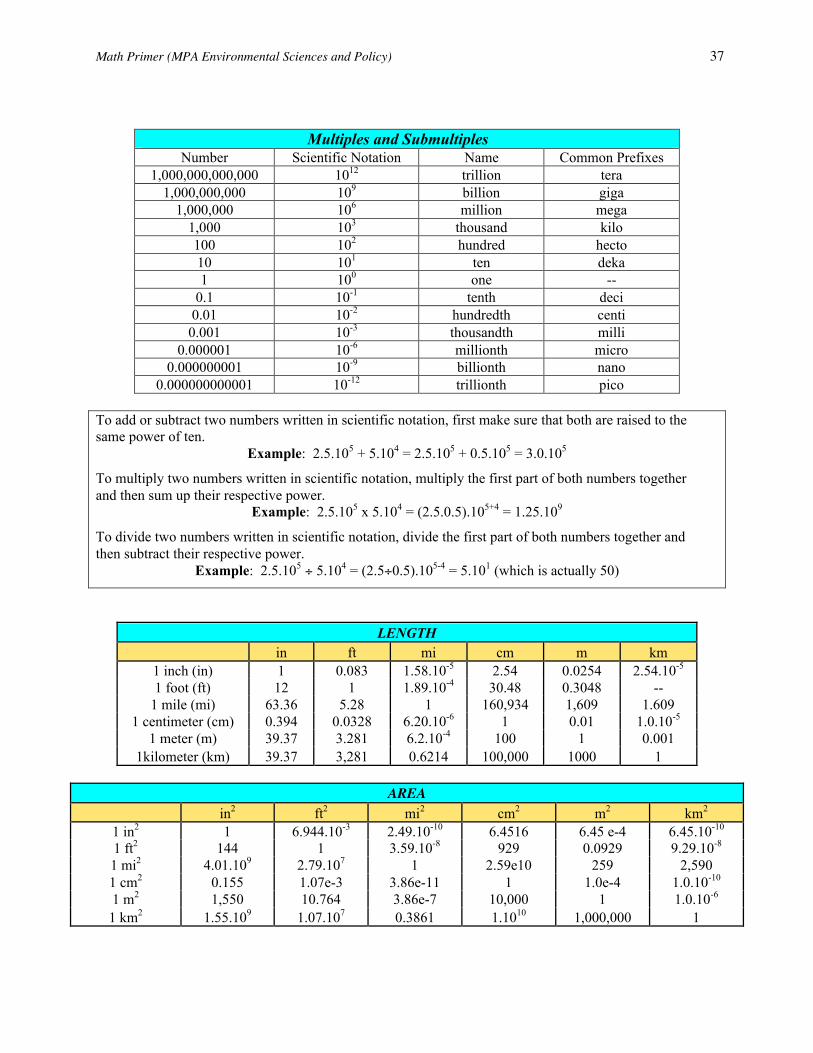
Math Primer (MPA Environmental Sciences and Policy) 37
Multiples and SubmultiplesNumber Scientific Notation Name Common Prefixes
1,000,000,000,000 1012 trillion tera1,000,000,000 109 billion giga
1,000,000 106 million mega1,000 103 thousand kilo100 102 hundred hecto10 101 ten deka1 100 one --
0.1 10-1 tenth deci0.01 10-2 hundredth centi0.001 10-3 thousandth milli
0.000001 10-6 millionth micro0.000000001 10-9 billionth nano
0.000000000001 10-12 trillionth pico
To add or subtract two numbers written in scientific notation, first make sure that both are raised to thesame power of ten.
Example: 2.5.105 + 5.104 = 2.5.105 + 0.5.105 = 3.0.105
To multiply two numbers written in scientific notation, multiply the first part of both numbers togetherand then sum up their respective power.
Example: 2.5.105 x 5.104 = (2.5.0.5).105+4 = 1.25.109
To divide two numbers written in scientific notation, divide the first part of both numbers together andthen subtract their respective power.
Example: 2.5.105 ÷ 5.104 = (2.5÷0.5).105-4 = 5.101 (which is actually 50)
LENGTHin ft mi cm m km
1 inch (in) 1 0.083 1.58.10-5 2.54 0.0254 2.54.10-5
1 foot (ft) 12 1 1.89.10-4 30.48 0.3048 --1 mile (mi) 63.36 5.28 1 160,934 1,609 1.609
1 centimeter (cm) 0.394 0.0328 6.20.10-6 1 0.01 1.0.10-5
1 meter (m) 39.37 3.281 6.2.10-4 100 1 0.0011kilometer (km) 39.37 3,281 0.6214 100,000 1000 1
AREAin2 ft2 mi2 cm2 m2 km2
1 in2 1 6.944.10-3 2.49.10-10 6.4516 6.45 e-4 6.45.10-10
1 ft2 144 1 3.59.10-8 929 0.0929 9.29.10-8
1 mi2 4.01.109 2.79.107 1 2.59e10 259 2,5901 cm2 0.155 1.07e-3 3.86e-11 1 1.0e-4 1.0.10-10
1 m2 1,550 10.764 3.86e-7 10,000 1 1.0.10-6
1 km2 1.55.109 1.07.107 0.3861 1.1010 1,000,000 1

Math Primer (MPA Environmental Sciences and Policy) 38
VOLUMEin3 ft3 yd3 m3 qt liter barrel gal(U.S)
1 in3 1 5.79.10-4 2.14.10-5 1.64.10-5 1.73.10-2 0.02 -- 4.33.10-3
1 ft3 1,728 1 3.70e-3 0.0283 29.922 28.3 -- 7.481 yd3 46656 27 1 0.76 807.89 764.55 -- 201.971 m3 61,020 35.315 1.307 1 -- 1,000 -- --
1 quart (qt) 57.75 3.34.10-2 1.24.10-3 9.46.10-4 1 0.95 -- 0.251 liter (l) 61.02 3.53.10-2 1.31.10-3 1.0.10-3 1.06 1 -- 0.2642
1 barrel (oil) -- -- -- -- 168 159.6 1 421 gallon (U.S) 231 0.13 4.95.10-3 3.78.10-3 4 3.785 0.02 1
MASS AND WEIGHT1 pound 1 gram 1 short pound 1 long ton
453.6 grams 0.0353 ounce 2000 pounds 2240 pounds0.4536 Kg 0.0022 pound 907.2 kilograms 1008 kilograms16 ounces
1 metric ton 1 kilogram2205 pounds 2.205 pounds
1000 kilograms
TEMPERATUREFahrenheit to Celsius °F = (
†
95 x °C) + 32
Celsius to Fahrenheit °C = 9
5 x (°F – 32)
Kelvin to Celsius °K = °C + 273Celsius to Kelvin °C = °K - 273

Math Primer (MPA Environmental Sciences and Policy) 39
ReferencesAber and Melillo, 2001: Terrestrial Ecosystems; Academic Press, London, UK
Brennan, J.W. “Understanding Algebra - An online algebra text”: http://www.jamesbrennan.org/algebra/
Gerstman, B. and M. Innovera “StatPrimer, Version 5.3 - An online, public-domain biostatisticsinstructional manual”: http://www.sjsu.edu/faculty/gerstman/StatPrimer/
Gould, S.J. (1996) “Full House: The spread of excellence from Plato to Darwin”, Random House Inc.NY, NY
Gravetter, F.J. and L.B. Wallnau. (2000). Statistics for the Behavioral Sciences. Fifth Edition. WadsworthThompson Learning.