A Lyapunov Function Based Remedial Action Screening Tool Using Real‐Time Data

Prof. Joydeep MitraElectrical & Computer Engineering

Michigan State UniversityEast Lansing, MI 48824

(517) 353‐8528mitraj@msu.edu

1

• Following a potentially destabilizing event, the grid can evolve along any of numerous possible trajectories. Appropriate operator action can stabilize the system.

• Most real‐time tools today are based on steady state analysis. Transient stability analysis is computationally intensive, and emergency/remedial actions are prescribed using off‐line studies. 

• We are developing a screening tool that uses an approach based on Lyapunov functions to enable, without time‐domain simulation, the selection of appropriate remedial actions that are most likely to result in stabilizing trajectories. 

• Since the system evolves continuously, it is necessary to update the tool using real‐time data from the SCADA/EMS.

• Our tool will screen contingencies for stability and prescribe remedial action at real‐time speed.

Context/Vision 

2

3

Presentation Outline  Project Vision

Significance and impact Project components and deliverables Project team

Technical Approach Lyapunov stability and screening; homotopy‐based approach System modeling and energy function Polynomial Lyapunov function Control actions

Results and Technical Accomplishments Screening by homotopy Polynomial Lyapunov functions Control actions Real‐time simulation status Visualization

Plans and Expectations Conclusion  Acknowledgments/Contacts

4

• The past decade has witnessed a higher frequency of grid disruptions in the North American Grid than any other similar period in history.

• A key finding of NERC’s Technical Analysis of the August 14, 2003 Blackoutis that grid operators needed increased situational awareness, and improved understanding of remedial action alternatives.

• The need for better situational awareness fueled a multitude of activities that are part of various “smart grid” initiatives.

• The L‐RAS will select appropriate remedial actions for the system operator to stabilize the system and represent a significant mathematical innovation toward enabling the understanding of catastrophic failure in power systems and the rapid and correct selection of remedial actions.

• The algorithms will be tested on a utility system (Southern California Edison) simulated on a real‐time digital simulation cluster, and the software and interface will be vetted by utility (SCE) personnel.

Significance and Impact

Project Components/Tasks

1. Development of a methodology for contingency screening using a homotopy method based on Lyapunov functions and real‐time data.

2. Development of a polynomial Lyapunov function that is capable of capturing a larger region of attraction than the energy functions that have been traditionally used in power systems.

3. Development of a methodology for recommending strategic and tactical remedial action recommendations based on the screening results.

4. Development of a visualization and operator interface tool.5. Testing of screening tool, validation of control actions, and 

demonstration of project outcomes on a representative real system simulated on a Real‐Time Digital Simulator (RTDS®) cluster.

5

Project Deliverables

1. A software prototype tested on a simulated system, vetted by utility personnel, and potentially ready for wider testing and commercialization

2. An RTDS‐based test bed that can be used for future research in the field 

3. A suite of breakthrough theoretical contributions to the field of power system stability and control

4. A new tool for visualization of power system stability margins

6

Project Team

7

Lead Institution: Michigan State University (MSU)Principal Investigator: Prof. Joydeep Mitra, MSUPartners: University of Illinois–Chicago (UIC), Los Alamos National Lab (LANL), Florida State University Center for Advanced Power Systems (FSU‐CAPS), Southern California Edison (SCE), LCG Consulting (LCG)

Co‐Investigators:Prof. Sudip K Mazumder, UICDr. Scott Backhaus, LANLDr. Russell Bent, LANLDr. Feng Pan, LANLDr. Manuel Garcia, LANLProf. Omar  Faruque, FSUDr. Mischa Steurer, FSUDr. Benyamin Moradzadeh, LCGSidart Deb, LCGDr. Nagy Abed, SCEFrank Ashrafi, SCE

Technical Approach: Summary

8

• This project will develop an advanced computational tool to assist system operators in making real‐time redispatch decisions to preserve power grid stability. 

• The tool will enable transient stability evaluation at real‐time speed without the use of massively parallel computational resources. 

• Traditional time domain simulation employed in transient stability analysis is computationally intensive. It is difficult to analyze a large number of trajectories to determine stability at real‐time speed.

• To avoid time domain simulation, this project uses homotopy and Lyapunov functions to screen out stable trajectories. Only a small number of trajectories will be subjected to time domain simulation.

• The trajectories will be updated as necessary with real‐time data.• Based on the screening results, control actions will be developed to stabilize the system.

Lyapunov Function and Region of Attraction

9

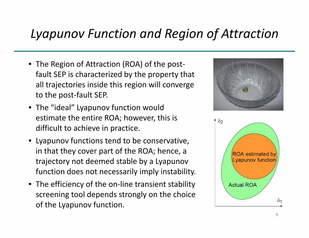
• The Region of Attraction (ROA) of the post‐fault SEP is characterized by the property that all trajectories inside this region will converge to the post‐fault SEP. 

• The “ideal” Lyapunov function would estimate the entire ROA; however, this is difficult to achieve in practice. 

• Lyapunov functions tend to be conservative, in that they cover part of the ROA; hence, a trajectory not deemed stable by a Lyapunovfunction does not necessarily imply instability.

• The efficiency of the on‐line transient stability screening tool depends strongly on the choice of the Lyapunov function.

Controlling Unstable Equilibrium Point

10

coX

)( coXR

)( cos XW

)( sXA

)( sXA

sXpresX

EP: Exit Point 

MGP: Minimum Gradient Point 

Xco: Controlling UEP 

R(Xco): Region of Convergence of the controlling UEP 

Xs: Post‐Fault SEP 

Xspre : Pre‐Fault SEP 

A(Xs): Region of Attraction of Post‐Fault SEP – ROA 

∂A(Xs): Boundary of the Region of Attraction of Post‐Fault SEP 

Ws(Xco): Stable Manifold of the controlling UEP 

Technical Approach: Screening

11

List of contingencies

Unstable contingency

All contingencies

screened?

Yes

End

i=i+1

Stable contingencies

Islanding problem?

No

Contingency i

No

Yes

Satisfied

Stable?

Yes

No

Other criteriaNot

satisfied

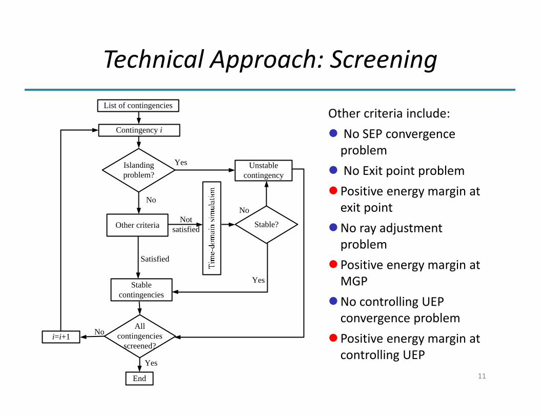
Other criteria include: No SEP convergence problem

No Exit point problemPositive energy margin at exit point

No ray adjustment problem

Positive energy margin at MGP

No controlling UEP convergence problem

Positive energy margin at controlling UEP

Homotopy‐based approaches

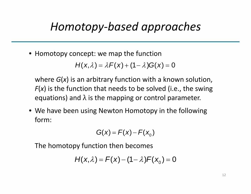
• Homotopy concept: we map the function

where G(x) is an arbitrary function with a known solution, F(x) is the function that needs to be solved (i.e., the swing equations) and λ is the mapping or control parameter.

• We have been using Newton Homotopy in the following form:

The homotopy function then becomes

12

( , ) ( ) (1 ) ( ) 0H x F x G x

0( ) ( ) ( )G x F x F x

0( , ) ( ) (1 ) ( ) 0H x F x F x

Role of Homotopy in Screening

• Homotopy‐based approaches map the trajectory of the solution (in this case the controlling UEP) from a known and easy to find solution (starting point). The starting points can be the exit points or the minimum gradient points (MGP) whichever is available.

• Homotopy‐based approaches are used to avoid to the extent possible the use of time‐domain simulations for the cases where numerical problems arise. Homotopy‐based approaches are used in these scenarios:– Numerical problems in precise determination of the Exit Points or other uncertainty

– The MGP cannot be detected – Iterative methods fail to calculate the controlling UEP

13

System Modeling I

14

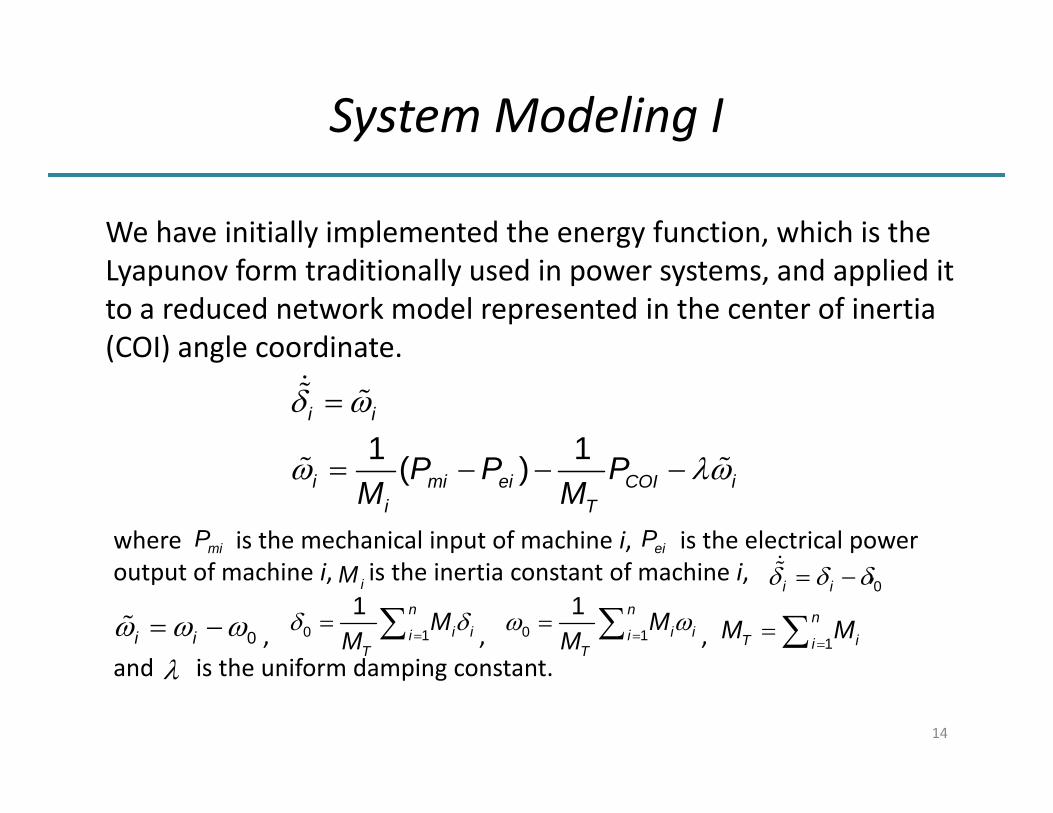
We have initially implemented the energy function, which is the Lyapunov form traditionally used in power systems, and applied it to a reduced network model represented in the center of inertia (COI) angle coordinate.

i i

1 1( )i mi ei COI ii T

P P PM M

where         is the mechanical input of machine i,        is the electrical power output of machine i,      is the inertia constant of machine i,                    , 

,                                   ,                                    ,                             and       is the uniform damping constant.

miP eiP

iM 0i i

0i i 0 1

1 ni ii

T

MM

0 1

1 ni ii

T

MM

1

nT ii

M M

System Modeling II

15

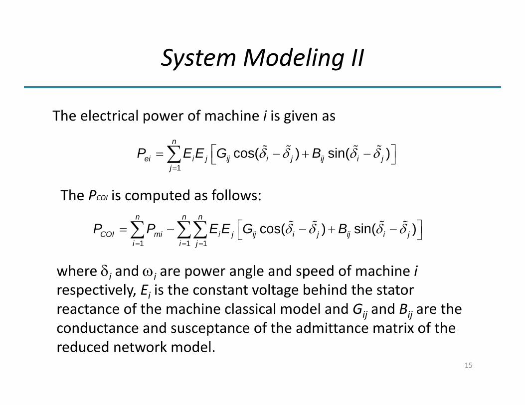
The electrical power of machine i is given as

where i and i are power angle and speed of machine irespectively, Ei is the constant voltage behind the stator reactance of the machine classical model and Gij and Bij are the conductance and susceptance of the admittance matrix of the reduced network model.

The PCOI is computed as follows:

1cos( ) sin( )

n

ei i j ij i j ij i jj

P E E G B

1 1 1cos( ) sin( )

n n n

COI mi i j ij i j ij i ji i j

P P E E G B

Energy Function

16

The transient energy function is expressed as

where

12

1 1 1 1

1 ( ) (cos cos )2

n n n ns s

i i i i i ij ij ij iji i i j i

V M P C I

2i mi i iiP P E G

Iij is the energy dissipated in the network transfer conductancesand can be expressed as

cosi j

s si j

ij ij ij i jI D d

This term is path dependent and can be calculated only if the system trajectory is known. It is common to use the following approximation:

sin sins s

i j i j sij ij ij ijs s

i j i j

I D

Technical Approach: Polynomial Lyapunov Fn.

17

Purpose: To develop a polynomial Lyapunov function that can include losses, and potentially accommodate switching functions and other non‐linearities .

Algorithm for PLF

18

0

Step 1: Obtaining upper bound  of V(x) such thatincluded in  0 such that

Step 2: Determining the largest  such that:p x included in 

0

p x

Step 3: Determining a V(x) such thatincluded between 0

and p x

0

· is SOS

is SOS

is SOS· is SOS

is SOS

Technical Approach: Control Actions

19

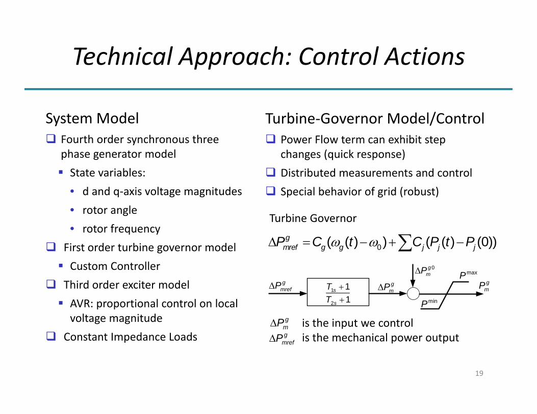
System Model Fourth order synchronous three 

phase generator model State variables:

• d and q‐axis voltage magnitudes• rotor angle• rotor frequency

First order turbine governor model Custom Controller

Third order exciter model AVR: proportional control on local voltage magnitude

Constant Impedance Loads

Turbine‐Governor Model/Control Power Flow term can exhibit step 

changes (quick response) Distributed measurements and control Special behavior of grid (robust)

Turbine Governor

0( ( ) ) ( ( ) (0))gmref g g j j jP C t C P t P

is the input we controlis the mechanical power output g

mrefP

gmP

1

2

11

s

s

TT

gmrefP g

mP

0gmP

gmP

maxP

minP

Results and Technical Accomplishments

1. The fundamental theoretical development of homotopy‐based screening tool has been completed using traditional energy functions, and tested in the IEEE 39‐bus test system.

2. The fundamental theoretical development of a polynomial Lyapunovfunction suitable for power system stability analysis has been completed and tested on several small test systems.

3. A methodology for evaluation of trajectory stability, and control strategies for stabilization of sets of potentially unstable trajectories, have been developed and are being tested.

4. A preliminary version of a visualization tool had been developed.5. The IEEE 39‐bus test case has been implemented on an RTDS cluster. 

Several PMU cards have been procured and installed on the cluster, and streaming of PMU data from CAPS and acquisition at MSU had been tested.

20

Test Systems Used

21

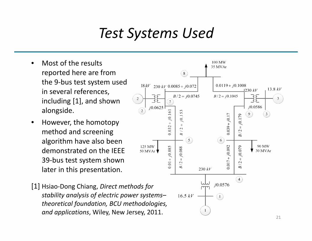
• Most of the results reported here are from the 9‐bus test system used in several references, including [1], and shown alongside.

• However, the homotopymethod and screening algorithm have also been demonstrated on the IEEE 39‐bus test system shown later in this presentation.

[1] Hsiao‐Dong Chiang, Direct methods for stability analysis of electric power systems–theoretical foundation, BCU methodologies, and applications, Wiley, New Jersey, 2011.

Results: Screening by Homotopy Method

22

Contingency number 

Fault at Bus 

Line Trip  Exit points ( 1 ,  2,  3)(rad) From  To 

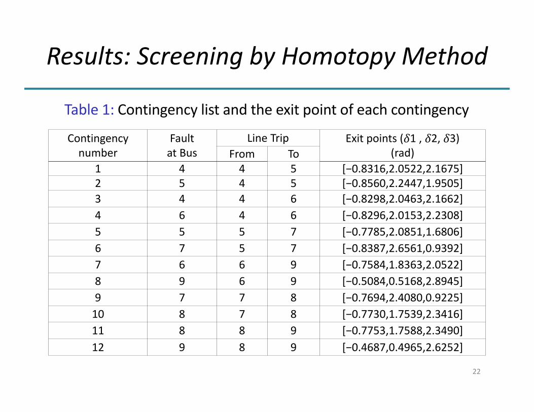
1  4  4  5  [−0.8316,2.0522,2.1675] 2  5  4  5  [−0.8560,2.2447,1.9505] 3  4  4  6  [−0.8298,2.0463,2.1662] 4  6  4  6  [−0.8296,2.0153,2.2308] 5  5  5  7  [−0.7785,2.0851,1.6806] 6  7  5  7  [−0.8387,2.6561,0.9392] 7  6  6  9  [−0.7584,1.8363,2.0522] 8  9  6  9  [−0.5084,0.5168,2.8945] 9  7  7  8  [−0.7694,2.4080,0.9225] 10  8  7  8  [−0.7730,1.7539,2.3416] 11  8  8  9  [−0.7753,1.7588,2.3490] 12  9  8  9  [−0.4687,0.4965,2.6252] 

Table 1: Contingency list and the exit point of each contingency 

Results: Screening by Homotopy II

23

Table 2: Controlling UEP obtained by homotopy method Contingency number  CUEP from homotopy  CUEP from [1] 

1 [−0.8323, 2.0742, 2.1447]  [−0.8364, 2.0797, 2.1466] 2 [−0.8323, 2.0742, 2.1447]  [−0.8364, 2.0797, 2.1466] 3 [−0.8266, 2.0821, 2.0540]  [−0.8256, 2.0830, 2.0549] 4 [−0.8266, 2.0821, 2.0540]  [−0.8256, 2.0830, 2.0549] 5 [−0.7598, 1.9521, 1.8071]  [−0.7589, 1.9528, 1.8079] 6 [−0.7598, 1.9521, 1.8071]  [−0.7589, 1.9528, 1.8079] 7 [−0.7586, 1.8576, 1.9979]  [−0.7576, 1.8583, 1.9986] 8 [−0.7586, 1.8576, 1.9979]  [−0.7576, 1.8583, 1.9986] 9 [−0.5430, 2.1797, −0.3764]  [−0.5424, 2.1802, −0.3755] 10 [−0.3500, 0.0738, 2.5861]  [−0.3495, 0.0745, 2.5864] 11 [−0.2915, −0.1017, 2.5004]  [−0.2910, −0.1011, 2.5008] 12 [−0.2915, −0.1017, 2.5004]  [−0.2910, −0.1011, 2.5008] 

[1] Hsiao‐Dong Chiang, Direct methods for stability analysis of electric power systems–theoretical foundation, BCU methodologies, and applications, Wiley, New Jersey, 2011. 

Results: Screening by Homotopy III

24

Table 3: The use of program components in the screening process in case of disturbing the exit points

Contingency number 

Stable/ Unstable 

Use of program components 

Iterative methods  Homotopy  Time‐domain 1  stable  –2  stable  –3  stable  –4  stable  –5  – stable 6  unstable  –7  stable  –8  unstable  –9  – unstable 10  stable  –11  stable  –12  unstable  –

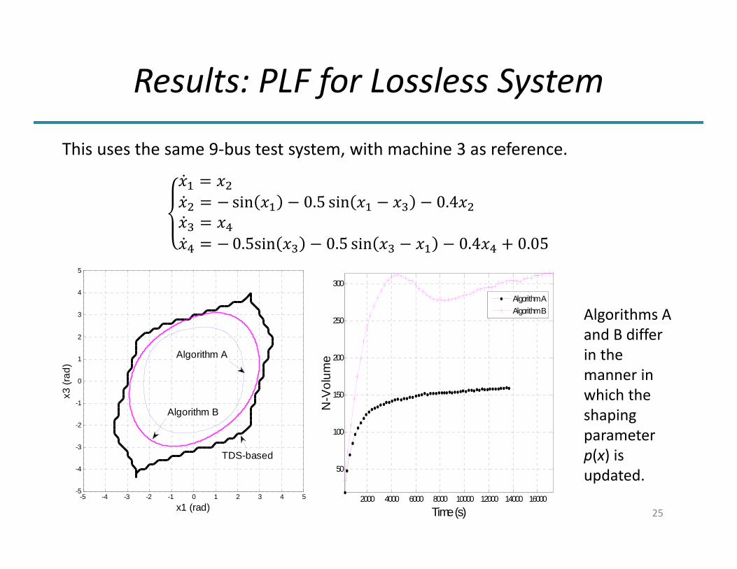
Results: PLF for Lossless System

25

sin 0.5 sin 0.4 0.5sin 0.5 sin 0.4 0.05

x1 (rad)

x3 (r

ad)

-5 -4 -3 -2 -1 0 1 2 3 4 5

-5

-4

-3

-2

-1

0

1

2

3

4

5

Algorithm A

Algorithm B

TDS-based

2000 4000 6000 8000 10000 12000 14000 16000

50

100

150

200

250

300

Time (s)

N-V

olum

e

Algorithm AAlgorithm B

This uses the same 9‐bus test system, with machine 3 as reference.

Algorithms A and B differ in the manner in which the shaping parameter p(x) is updated. 

Results: PLF for Lossy System

26

33.5849 1.8868cos 5.283cos 16.9811 sin 59.6226 sin 1.8868 48.4810 11.3924 sin 1.2658cos 3.2278 cos 99.3671 sin 1.2658

x1 (rad)

x3 (r

ad)

-2.5 -2 -1.5 -1 -0.5 0 0.5 1 1.5 2 2.5-2.5

-2

-1.5

-1

-0.5

0

0.5

1

1.5

2

2.5

Algorithm B

TDS-based

Algorithm A

1000 2000 3000 4000 5000 6000 7000

20

40

60

80

100

120

140

160

180

Time (s)

N-V

olum

e

Algorithm AAlgorithm B

Results: Optimized Control Actions

27

Penalty Terms:• Frequency dispersion among 

generators.          is the instantaneous average generator frequency. 

• Voltage deviation on every bus.

Figure : Penalty vs Duration Curve

0

2 2

0

0 0

( ) ( )( ) ( )1 ( )( )

ft i iit

i G i N i

V t V tt tP a t dtT V t

( )t

Optimization• Choose Threshold P using Penalty vs

Duration curve• Determine unstable faults U• Solve using gradient method

min min max( ,0)j j

mult i iC C i UP P P

Figure: Illustration of penalty terms

Results: Increasing System Load

28

Penalty will increase as system load increases. Assume load increases uniformly. 

Interpreting Plots: • begin by traversing 

droop control curve• perform update when 

penalty at bus 8 crosses threshold

• traverse step 1 curve until another fault crosses its threshold

• Top Left: Droop control curves for faults at bus 7, 8 and 9

• Other Three: Evolution of curve as control is updated

The 14‐rack RTDS system at FSU‐CAPS is being used as a surrogate for a real system to achieve the following:• Validate the accuracy and effectiveness of the proposed 

Lyapunov function based algorithm by mimicking the dynamic behavior of power system using real‐time simulation. 

• Demonstration of the robustness of the algorithm for contingency analysis.

Real‐Time Digital Simulation 

29

LRAS Tool with Visualization (at MSU end)

InternetIEEE C37.118 protocol

Real‐time Simulation Modelat FSU end

30

Validation Strategy: Summary

4. Overall performance validation and evaluation4. Overall performance validation and evaluation

Comprehensive testing using LRAS tool and PMU data streaming in real‐time over the Internet 

Demonstration of the algorithm in contingency analysis by feeding real‐time data from PMU streaming

3. PMU measurement data streaming through the Internet3. PMU measurement data streaming through the Internet

Using Internet as the communication media Bi‐directional data communication between MSU and FSU using VPN or secured networking

2. Hardware and software installation for PMU streaming2. Hardware and software installation for PMU streaming

Installation of PMU hardware and firmware on RTDS Platform for streaming phasor data from the real‐time simulation using the standard IEEE C37.118 protocol

1. Real‐time Simulation Model Development1. Real‐time Simulation Model Development

Model conversion from PSSE to RTDS and Validation  using IEEE 39 Test Bus

Model conversion/development and validation of actual SCE System

p

Status: Developed and validated theIEEE 39 BUS test system in RTDS. Nextstep is to develop the model of actualSCE system. Waiting on SCE data andLRAS tool development

Status: Installation and testing iscomplete. Capable of streaming 96PMU data from different location ofthe network.

Status: One way data communicationbetween FSU and MSU and testing iscomplete; working on making it bi‐directional

Status: In progress.

31

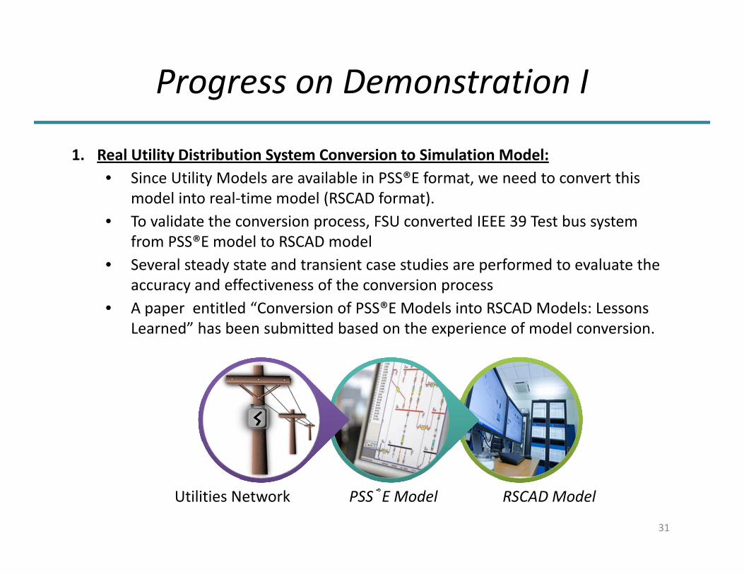
Progress on Demonstration I

1. Real Utility Distribution System Conversion to Simulation Model:• Since Utility Models are available in PSS®E format, we need to convert this 

model into real‐time model (RSCAD format).• To validate the conversion process, FSU converted IEEE 39 Test bus system 

from PSS®E model to RSCAD model• Several steady state and transient case studies are performed to evaluate the 

accuracy and effectiveness of the conversion process • A paper  entitled “Conversion of PSS®E Models into RSCAD Models: Lessons 

Learned” has been submitted based on the experience of model conversion.

Utilities Network PSS®E Model RSCAD Model

32

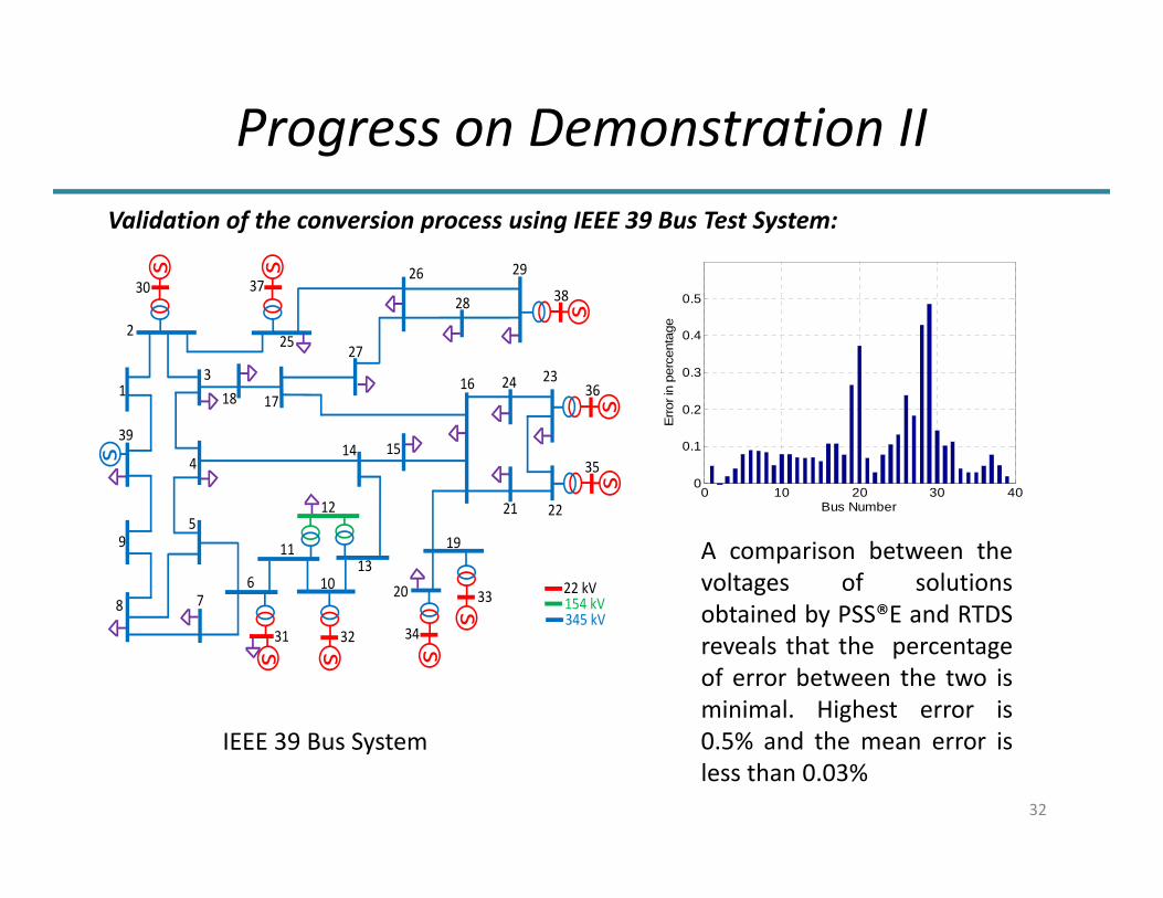
Progress on Demonstration II

  s s

s

ssss

ss

30

1

2

318 17

25

26 29

383728

27

39

9

8

5

4

76

11

10

14 15

16 24

21

31 32 34

20

19

33

22

2336

35

12

1322 kV154 kV345 kV

0 10 20 30 400

0.1

0.2

0.3

0.4

0.5

Bus Number

Erro

r in

perc

enta

ge

A comparison between thevoltages of solutionsobtained by PSS®E and RTDSreveals that the percentageof error between the two isminimal. Highest error is0.5% and the mean error isless than 0.03%

IEEE 39 Bus System

Validation of the conversion process using IEEE 39 Bus Test System:

33

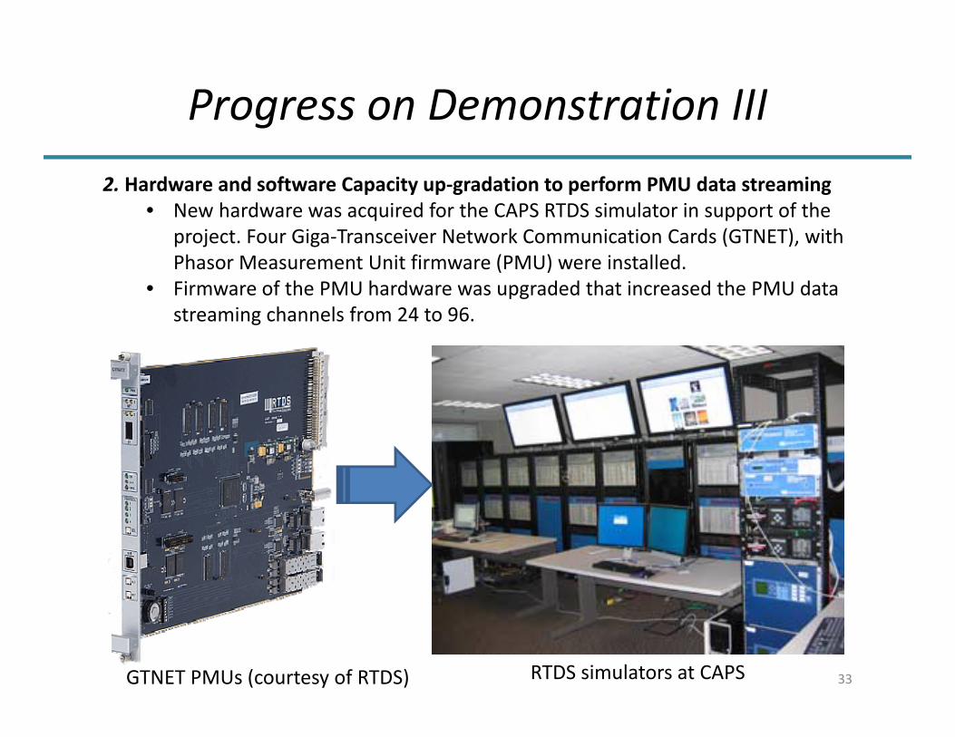
Progress on Demonstration III2. Hardware and software Capacity up‐gradation to perform PMU data streaming

• New hardware was acquired for the CAPS RTDS simulator in support of the project. Four Giga‐Transceiver Network Communication Cards (GTNET), with Phasor Measurement Unit firmware (PMU) were installed.

• Firmware of the PMU hardware was upgraded that increased the PMU data streaming channels from 24 to 96.

RTDS simulators at CAPSGTNET PMUs (courtesy of RTDS)

34

Progress on Demonstration IV3. PMU measurement data streaming through Internet

• Test cases were executed using the IEEE 39 Bus system.• Four fault cases were created and PMU measurement of Voltage and Current 

data for 32 Buses were streamed through the Internet.• FSU has streamed the data over the Internet to MSU who received those PMU 

data remotely using open source software named “PMU connection tester” and saved the data for further analysis.

Fig. IEEE 39 Bus System with Fault locations and PMU connections

Visualization Scheme

35

The following data is communicated and updated every 4 seconds• Bus data: Bus ID, Name, Latitude, Longitude, Nominal Voltage, Real Power Load,  Reactive Power Load, Angle, Voltage, Frequency 

• Generator data: Generator ID, Generator Name, Bus ID,  Pmin,  Pmax, Qmin,  Qmax,  Real Power,  Reactive Power 

• Lines data: Line ID, Name, From Bus ID,  To Bus ID, Limit,  Active Power Flow, Reactive Power Flow 

• Interfaces: Interface ID, Interface Name, Forward Limit, Reverse Limit, Flow • Interface lines: Interface ID, Line, Coefficient • Bus warning: Bus ID, Warning • Line warning: Line ID, Description • Bus fault: Bus ID, Description • Line fault: Line ID, Description 

Visualization: Illustration

36

Plans and Expectations

The near‐term plans and next steps for the project components are as follows.1. The homotopy‐based method is being developed into a multi‐parameter, 

variable‐gain form for increased computational efficiency. This will then be tested on several large test systems.

2. After testing the polynomial Lyapunov method and the control strategies on larger systems, these will be integrated with the homotopy‐based screening algorithm.

3. The screening algorithm will be modified to accept and use real‐time data streamed from the RTDS cluster at FSU‐CAPS. The control algorithm will be sent to CAPS for testing on the RTDS.

4. SCE is developing a reduced model of their system for implementation on the RTDS cluster.

5. LCG is developing a user interface to integrate with the visualization tool. This visualization and user‐interface tool will be integrated with the screening and control algorithm for final testing, demonstration, and vetting by the team, including utility personnel.

37

38

Conclusion 

• This project has many components under development in parallel and these have progressed well. 

• New theoretical contributions that were anticipated have also produced promising results: Homotopy method Polynomial Lyapunov function Distributed control actions 

• A preliminary visualization tool has also been developed. • The work performed has been kept in alignment with input from 

industry partners.• Integration and demonstration tasks that remain are expected to be 

completed by September 2015.• We are excited about this project and look forward to producing an 

integrated and potentially commercializable product.

39

Financial support is acknowledged from the US Department of Energy.

Technical contributions from the following are appreciated:  Collaborators:

• Prof. Sudip K. Mazumder, mazumder@uic.edu• Dr. Scott Backhaus, backhaus@lanl.gov• Prof. Omar Faruque, faruque@caps.fsu.edu• Dr. Benyamin Moradzadeh, moradzadeh@energyonline.com

And my graduate students:• Mohammed Benidris• Niannian Cai• Nga Nguyen

Principal Investigator: Prof. Joydeep Mitra, mitraj@msu.edu

Acknowledgements/Contacts

A Lyapunov Function Based Remedial Action Screening Tool Using Real‐Time Data

Key Personnel: Joydeep Mitra (Michigan State University), Sudip K. Mazumder (University of Illinois–Chicago), Scott N. Backhaus (Los Alamos National Lab), Omar Faruque (Florida State University), Sidart Deb (LCG Consulting), Nagy Abed (Southern California Edison)

Purpose of Project: To develop an advanced computational tool that is will assist system opera‐tors in making real‐time redis‐patch decisions to preserve power grid stability. The tool relies on screening contingencies using a homotopy method based on Lyapunov functions to avoid, to the extent possible, the use of time domain simulations. This enables transient stability eval‐uation at real‐time speed with‐out the use of massively parallel computational resources. The tool is updated with real‐time data as the contingency evolves.

Key Innovations:• A new methodology for 

contingency screening using a homotopy approach based on Lyapunov func‐tions and real‐time data.

• A polynomial Lyapunovfunction capable of captur‐ing a larger region of attrac‐tion than energy functions.

• A methodology for recom‐mending strategic and tactical remedial action recommendations based on the screening results.

• A novel visualization and operator interface tool.

Deliverables:• A software proto‐

type ready for commercialization

• A real‐time digital simulation test‐bed

• A suite of break‐through theoretical contributions on grid stability and control

• A new visualization tool for grid stability

Budget:DOE: $1,500,000Cost‐share: $375,000Total: $1,875,000  40