A Low Cost Method to Develop an Initial Pavement ... · I A Low Cost Method to Develop an Initial Pavement Management System A Thesis in The Department of Building, Civil and Environmental

I

A Low Cost Method to Develop an Initial Pavement

Management System

A Thesis

in

The Department of

Building, Civil and Environmental Engineering

Presented in Partial Fulfillment of the Requirements for the

Degree of Master of Applied Science

at

Concordia University

Montreal, Quebec, Canada

February 2014

© Mohammed Al-Dabbagh, 2014

II

CONCORDIA UNIVERSITY

School of Graduate Studies This is to certify that the thesis prepared By: Mohammed Al-Dabbagh Entitled: A Low Cost Method to Develop an Initial Pavement Management

System and submitted in partial fulfillment of the requirements for the degree of

Master of Applied Science (Civil Engineering) complies with the regulations of the University and meets the accepted standards with respect to originality and quality. Signed by the final examining committee:

__________________________________________________ Chair Dr. S. Samuel Li __________________________________________________ Examiner Dr. Fariborz Haghighat __________________________________________________ External Examiner Dr. Deborah Dysart-Gale __________________________________________________ Supervisor

Dr. Luis Amador Approved by

______________________________________________ Chair of Department or Graduate Program Director

______________________________________________

Dean of Faculty Date _____________________________________________

III

ABSTRACT

A Low Cost Method to Develop an Initial Pavement Management System

Mohammed Al-Dabbagh

Implementation of a pavement management system requires data collection to estimate

system needs, performance modeling to forecast time sensitive changes and decision

making to allocate interventions. Many agencies have embarked into the implementation

of a pavement management system which eventually after some years render its fruits,

however, implementation typically involves expensive equipment, years of data collection

and hundreds of hours of workmanship. This all result in a barrier that impedes

implementation at small municipalities and governments in developing countries. A low

cost solution to estimate road surface roughness condition and to implement an initial

pavement management system is proposed in this research. Pavement roughness can be

estimated with an accelerometer built-in tablets and smart phones. Vertical accelerations

normalized by speed can be used to produce a proxy for International Roughness Index.

Testing of the method was done by comparing different tablets, applications, vehicles,

speeds and location of the instrument inside the vehicle. Performance models were

developed using World Bank’s equation of IRI, road repair strategies were correlated to

testing sections in need of maintenance or rehabilitation repairs. This research shows a case

study of the town of Saint-Michelle in Quebec. Data was collected for all municipal roads

in Saint Michelle and a pavement management system was developed. It was found that

$254,418 dollars is required in order to sustain current levels of condition. It is

recommended that in the future performance models are based on several years of

observations in order to replace the synthetic deterministic curves herein adopted.

IV

DEDICATION

To my wife: Hind, my daughter: Reema and my son: Ibrahim

V

ACKNOWLEDGEMENT

I would like to express my sincere gratitude to my supervisor Dr. Luis Amador for his

advice, guidance and continuous support during all the time of research and writing of this

thesis. I was so honored to work under his supervision.

I would like also to express my appreciation to the examining committee: Dr.

Fariborz Haghighat, Dr. Deborah Dysart-Gale, and Dr. S. Samuel Li.

VI

TABLE OF CONTENTS

TABLE OF CONTENTS .................................................................................................. VI

LIST OF FIGURES ....................................................................................................... VIII

LIST OF TABLES ............................................................................................................. X

LIST OF ABBREVIATIONS ........................................................................................... XI

CHAPTER 1 ....................................................................................................................... 1

INTRODUCTION .............................................................................................................. 1

1.1 Background ............................................................................................................... 1

1.2 Problem Statement .................................................................................................... 2

1.3 Research Objective ................................................................................................... 3

1.3.1 Overall Goal ∙∙∙∙∙∙∙∙∙∙∙∙∙∙∙∙∙∙∙∙∙∙∙∙∙∙∙∙∙∙∙∙∙∙∙∙∙∙∙∙∙∙∙∙∙∙∙∙∙∙∙∙∙∙∙∙∙∙∙∙∙∙∙∙∙∙∙∙∙∙∙∙∙∙∙∙∙∙∙∙∙∙∙∙∙∙∙∙∙∙∙∙∙∙∙∙∙∙∙∙∙∙ 3

1.3.2 Specific Objectives ∙∙∙∙∙∙∙∙∙∙∙∙∙∙∙∙∙∙∙∙∙∙∙∙∙∙∙∙∙∙∙∙∙∙∙∙∙∙∙∙∙∙∙∙∙∙∙∙∙∙∙∙∙∙∙∙∙∙∙∙∙∙∙∙∙∙∙∙∙∙∙∙∙∙∙∙∙∙∙∙∙∙∙∙∙∙∙∙∙∙∙∙∙ 3

1.4 Scope and Limitations ............................................................................................... 3

1.5 Research Significance ............................................................................................... 4

1.6 Organization of the Thesis ........................................................................................ 4

CHAPTER 2 ....................................................................................................................... 5

LITERATURE REVIEW ................................................................................................... 5

2.1 Pavement Condition .................................................................................................. 5

2.1.1 Pavement Distress ∙∙∙∙∙∙∙∙∙∙∙∙∙∙∙∙∙∙∙∙∙∙∙∙∙∙∙∙∙∙∙∙∙∙∙∙∙∙∙∙∙∙∙∙∙∙∙∙∙∙∙∙∙∙∙∙∙∙∙∙∙∙∙∙∙∙∙∙∙∙∙∙∙∙∙∙∙∙∙∙∙∙∙∙∙∙∙∙∙∙∙∙∙∙ 6

2.1.2 Pavement Condition Indices ∙∙∙∙∙∙∙∙∙∙∙∙∙∙∙∙∙∙∙∙∙∙∙∙∙∙∙∙∙∙∙∙∙∙∙∙∙∙∙∙∙∙∙∙∙∙∙∙∙∙∙∙∙∙∙∙∙∙∙∙∙∙∙∙∙∙∙∙∙∙∙∙∙∙∙∙ 11

2.1.3 Pavement Roughness Evaluation ∙∙∙∙∙∙∙∙∙∙∙∙∙∙∙∙∙∙∙∙∙∙∙∙∙∙∙∙∙∙∙∙∙∙∙∙∙∙∙∙∙∙∙∙∙∙∙∙∙∙∙∙∙∙∙∙∙∙∙∙∙∙∙∙∙∙∙∙∙ 12

2.1.4 International Roughness Index (IRI) ∙∙∙∙∙∙∙∙∙∙∙∙∙∙∙∙∙∙∙∙∙∙∙∙∙∙∙∙∙∙∙∙∙∙∙∙∙∙∙∙∙∙∙∙∙∙∙∙∙∙∙∙∙∙∙∙∙∙∙∙∙∙∙ 14

2.2 Civil Infrastructure Asset Management .................................................................. 16

2.3 Pavement Management Systems ............................................................................. 17

2.4 Pavement Performance Prediction Modeling ......................................................... 19

2.4.1 Stochastic Model ∙∙∙∙∙∙∙∙∙∙∙∙∙∙∙∙∙∙∙∙∙∙∙∙∙∙∙∙∙∙∙∙∙∙∙∙∙∙∙∙∙∙∙∙∙∙∙∙∙∙∙∙∙∙∙∙∙∙∙∙∙∙∙∙∙∙∙∙∙∙∙∙∙∙∙∙∙∙∙∙∙∙∙∙∙∙∙∙∙∙∙∙∙∙ 20

2.4.2 Deterministic Model ∙∙∙∙∙∙∙∙∙∙∙∙∙∙∙∙∙∙∙∙∙∙∙∙∙∙∙∙∙∙∙∙∙∙∙∙∙∙∙∙∙∙∙∙∙∙∙∙∙∙∙∙∙∙∙∙∙∙∙∙∙∙∙∙∙∙∙∙∙∙∙∙∙∙∙∙∙∙∙∙∙∙∙∙∙∙∙∙∙ 22

2.5 Decision making for Pavement Management ......................................................... 31

2.5.1 Typical Mathematical Algorithms ∙∙∙∙∙∙∙∙∙∙∙∙∙∙∙∙∙∙∙∙∙∙∙∙∙∙∙∙∙∙∙∙∙∙∙∙∙∙∙∙∙∙∙∙∙∙∙∙∙∙∙∙∙∙∙∙∙∙∙∙∙∙∙∙∙∙∙∙ 31

2.5.2 Total Enumeration ∙∙∙∙∙∙∙∙∙∙∙∙∙∙∙∙∙∙∙∙∙∙∙∙∙∙∙∙∙∙∙∙∙∙∙∙∙∙∙∙∙∙∙∙∙∙∙∙∙∙∙∙∙∙∙∙∙∙∙∙∙∙∙∙∙∙∙∙∙∙∙∙∙∙∙∙∙∙∙∙∙∙∙∙∙∙∙∙∙∙∙ 33

VII

CHAPTER 3 ..................................................................................................................... 35

METHODOLOGY ........................................................................................................... 35

3.1 Introduction ............................................................................................................. 35

3.2 Road Roughness Measurement ............................................................................... 35

3.2.1 Data Collection Protocol ∙∙∙∙∙∙∙∙∙∙∙∙∙∙∙∙∙∙∙∙∙∙∙∙∙∙∙∙∙∙∙∙∙∙∙∙∙∙∙∙∙∙∙∙∙∙∙∙∙∙∙∙∙∙∙∙∙∙∙∙∙∙∙∙∙∙∙∙∙∙∙∙∙∙∙∙∙∙∙∙∙ 36

3.2.2 A Proxy for International Roughness Index ∙∙∙∙∙∙∙∙∙∙∙∙∙∙∙∙∙∙∙∙∙∙∙∙∙∙∙∙∙∙∙∙∙∙∙∙∙∙∙∙∙∙∙∙∙∙∙∙∙∙∙∙∙ 40

3.2.3 Normalization by speed ∙∙∙∙∙∙∙∙∙∙∙∙∙∙∙∙∙∙∙∙∙∙∙∙∙∙∙∙∙∙∙∙∙∙∙∙∙∙∙∙∙∙∙∙∙∙∙∙∙∙∙∙∙∙∙∙∙∙∙∙∙∙∙∙∙∙∙∙∙∙∙∙∙∙∙∙∙∙∙∙∙∙∙∙ 41

3.2.4 Comparison of Various Surface Conditions ∙∙∙∙∙∙∙∙∙∙∙∙∙∙∙∙∙∙∙∙∙∙∙∙∙∙∙∙∙∙∙∙∙∙∙∙∙∙∙∙∙∙∙∙∙∙∙∙∙∙∙∙ 46

3.2.5 Comparison of Applications and Devices Used for Data Collection ∙∙∙∙∙∙∙∙∙∙∙∙∙∙ 47

3.2.6 Comparison of Vehicles Sizes ∙∙∙∙∙∙∙∙∙∙∙∙∙∙∙∙∙∙∙∙∙∙∙∙∙∙∙∙∙∙∙∙∙∙∙∙∙∙∙∙∙∙∙∙∙∙∙∙∙∙∙∙∙∙∙∙∙∙∙∙∙∙∙∙∙∙∙∙∙∙∙∙∙∙ 49

3.2.7 Comparison of Sensor Locations ∙∙∙∙∙∙∙∙∙∙∙∙∙∙∙∙∙∙∙∙∙∙∙∙∙∙∙∙∙∙∙∙∙∙∙∙∙∙∙∙∙∙∙∙∙∙∙∙∙∙∙∙∙∙∙∙∙∙∙∙∙∙∙∙∙∙∙∙∙ 51

3.3 Database Preparation ............................................................................................... 52

CHAPTER 4 ..................................................................................................................... 55

CASE STUDY: TOWN OF SAINT-MICHELLE ........................................................... 55

4.1 Introduction ............................................................................................................. 55

4.2 Construction of Saint Michelle Road Spatial Database .......................................... 58

4.3 Construction of Performance Curves ...................................................................... 61

4.4 Estimation of Intervention Treatment Type and Effectiveness .............................. 64

4.5 Investment Strategies: allocation of funds and scheduling of levels of intervention per year .......................................................................................................................... 65

4.6 Optimization and Trade-off Analysis Results ......................................................... 66

CHAPTER 5 ..................................................................................................................... 73

CONCLUSIONS AND RECOMMENDATIONS ........................................................... 73

5.1 Conclusions ............................................................................................................. 73

5.2 Recommendations ................................................................................................... 75

References ......................................................................................................................... 76

VIII

LIST OF FIGURES

Figure 1: Sketch of pavement roughness in wheel-paths (Sayers & Karamihas, 1998) ..... 6

Figure 2: Block cracking (Pavemanpro.com, 2013) ........................................................... 8

Figure 3: Fatigue cracks (Butler, 2013) .............................................................................. 9

Figure 4: Transverse cracks (WAPA, 2013) ..................................................................... 10

Figure 5: Pavement rutting (Pavementinteractive, 2013) ................................................. 11

Figure 6: Laser pavement profilometer (Roadex, 2013) ................................................... 14

Figure 7: Operational framework for infrastructure management, including pavements (Hudson, et al., 1997) ........................................................................................ 19

Figure 8: An example of Markov Chain Performance Model for deterioration prediction (Amador & Mrawira, 2009) .............................................................................. 21

Figure 9: Uncertainty in pavement performance prediction curve (Amador & Mrawira, 2009) ................................................................................................................. 22

Figure 10: Logic sequence of road deterioration and maintenance submodel – paved roads (Watanatada, et al., 1987) ................................................................................. 29

Figure 11: Prediction of roughness progression for flexible and semi – rigid pavements under minimal maintenance of patching all the potholes (Watanatada, et al., 1987) ................................................................................................................. 30

Figure 12: Total enumeration process ............................................................................... 34

Figure 13: Standard Deviation of vertical acceleration with and without speed-normalization .................................................................................................... 36

Figure 14: Flow chart of data collection procedure .......................................................... 39

Figure 15: Comparison of speed-normalized standard deviation of z-accelerations – gravel – fair to good condition – same vehicle – various speeds ................................. 43

Figure 16: Comparison of speed-normalized standard deviations of z-accelerations – asphalt – poor condition – same vehicle – various speeds ................................ 44

Figure 17: Comparison of speed normalized standard deviations of z-accelerations – Earth – poor condition – same vehicle – various speeds ............................................ 45

Figure 18: Comparison of earth in fair- poor and asphalt in good condition.................... 46

Figure 19: Asphalt Good-Fair condition ........................................................................... 47

Figure 20: Comparison of observations – Iphone (SensorLog) vs Samsung (Physics Toolbox Accelerometer) ................................................................................... 48

Figure 21: Comparison of RI – segment in poor condition - various vehicles ................. 49

IX

Figure 22: Comparison of RI – segment in good condition – various vehicles ................ 50

Figure 23: Comparison of RI – same vehicle - same sensor at different locations........... 51

Figure 24: Point condition data-ARCGIS .......................................................................... 53

Figure 25: Database preparation flow chart ...................................................................... 54

Figure 26: Location of Saint-Michelle city (Google Maps) ............................................. 56

Figure 27: Saint-Michelle city (Google Maps) ................................................................. 56

Figure 28: Case study main work stages ........................................................................... 57

Figure 29: Constructing Saint Michelle road network database – flow chart ................... 60

Figure 30: Annual Average Daily Traffic (AADT) (TransportsQuebec, 2013) ............... 62

Figure 31: Pavement performance deterioration ............................................................... 63

Figure 32: Progression of very poor roads across time ..................................................... 69

Figure 33: Progression of condition groups across time ($350,000) ................................ 70

Figure 34: Annual intervention cost ($350,000) ............................................................... 71

Figure 35: Time progression of mean network condition ($350,000) .............................. 72

X

LIST OF TABLES Table 1: Definitions of variables used in HDM model (Watanatada, et al., 1987)........... 28

Table 2: Target speeds (kph) for tested surfaces............................................................... 42

Table 3: Interventions used in the analysis ....................................................................... 64

Table 4: Annual resource allocation per intervention type ............................................... 67

Table 5: Split of roads by condition group (in linear meters) ........................................... 67

XI

LIST OF ABBREVIATIONS

AADT Annual Average Daily Traffic

AASHTO American Association of State Highway and Transportation Officials

ASTM American Society of Testing and Materials

COST European Cooperation in the Field of Scientific and Technical Research

DOT Department of Transportation

ESAL Equivalent Single Axle Load

FHWA Federal Highway Administration

GPS Global Positioning System

HDM The Highway Design and Maintenance Standards Model

HMA Hot Mix Asphalt

IRI International Roughness Index

RI Roughness Indicator

TAC Transportation Association of Canada

UDOT Utah Department of Transportation

1

CHAPTER 1

INTRODUCTION

1.1 Background

An effective road network is a fundamental component of the economic and social

development of any country; therefore, pavements are one of the major investments

administered by governments around the world (Watanatada, et al., 1987). Maintenance

and rehabilitation has been identified as a key task to preserve pavements and ensure they

remain productive throughout their lifespan. They are also expensive (Posavljak, et al.,

2013).

First implementations of pavement management dates from the 1980’s with silo-type

systems for pavements (Tarpay, et al., 1996) (Chen, et al., 1996). Pavement management

was the precursor of bridges, water systems, and other assets management systems, which

are referred in general under the umbrella of asset management (Falls, et al., 2001).

Today Pavement Management Systems (PMS) are widely used by the governments

of many countries, provinces and states of developed countries (Chen, et al., 1996) (Falls,

et al., 2001). However they are no so common in poor countries or small municipalities

that lack the resources to implement them.

The implementation of a PMS is typically challenging task because it requires an

intensive data collection campaign (Khan, et al., 2003) which in turn necessitates utilization

of expensive equipment such as profilometers or deflectometers (Noureldin, et al., 2003).

2

Without such equipment, estimation of road condition is difficult if not impossible. Some

have used visual inspections in this circumstances (Amador & Magnuson, 2011), but visual

inspections suffer from two drawbacks: first are incapable of estimate the condition of the

structure and secondly are entirely related to human subjectivity which is an issue when

visiting thousands of kilometers of roads.

Another problem comes from the fact that treatment allocation should be based upon

a consistent repeatable criteria (Ksaibati, et al., 1999) which must relate to some

measurable indicator of damage (Mactutis, et al., 2000). The two most widely suggested

criteria are as rutting (also known as rut depth) and cracking (Hall & Muñoz, 1999).

Another difficulty to implement is the need to count with at least two condition data

points (Amador & Mrawira, 2011) traditionally recommending data collection for at least

5 years to observe trends. This because it requires the development of performance curves

(Falls, et al., 2001).

The final restriction comes from the fact that an optimization software is required in

order to support decision making for the allocation of resources and development of

strategic, tactical and operational plans (Posavljak, et al., 2013).

1.2 Problem Statement

There is a need to evaluate road condition with a low cost accessible method for small

municipalities and poor governments lacking the financial capability to develop and

implement a pavement management system.

3

1.3 Research Objective

1.3.1OverallGoal

Propose a low cost method to capture pavement surface condition and develop a low-cost

initial pavement management system.

1.3.2SpecificObjectives

1. Establish a low cost procedure to collect data for surface condition; and

2. Develop an initial pavement management systems based on a low-cost data-acquisition

method.

1.4 Scope and Limitations

This research proposes a low cost method to collect pavement surface condition data and

evaluate the pavement condition for the purpose of developing initial pavement

management system. Specifically, the research is limited to pavement surface roughness

assessment, although it is indirectly capable of incorporating structural decay when

observing time trends of longitudinal data collected across time. There is no

characterization of specific damage; however this is not required because operational

ranges for treatment allocation can be learnt from visiting deficient sections already

categorized to be in need of a specific type of intervention. No assessment of pavement

layers structural capacity or state of degradation is done, but this is not needed as surface

4

roughness is sufficient to be used in the decision criteria. Further testing will be required

to investigate the effect of horizontal and vertical curves in rebalancing of vertical

accelerations into horizontal accelerations.

1.5 Research Significance

This research makes the following contributions:

1. It proposes a method to evaluate surface condition of a pavement with a low cost

technology;

2. It proposes a procedure to establish an initial pavement management system in about a

year on the basis of low cost data acquisition; and

3. It demonstrates the method through a case study for municipal road network.

1.6 Organization of the Thesis

This thesis is presented in five chapters as follows; Chapter 1 defines the problem and

presents the objectives of the research and structure of the thesis. Chapter 2 displays a

review of concepts related to pavement management, specifically road surface condition,

performance curves and optimization to support decision making. Chapter 3 presents the

methodology employed for data collection. Chapter 4 presents a short case study

demonstrates the implementation of the proposed method for the purpose of dissemination

to potential users. Chapter 5 presents conclusions and recommendations, as well as

suggestions for future research.

5

CHAPTER 2

LITERATURE REVIEW

2.1 Pavement Condition

New pavements start out smooth and increase in roughness over the time (UDOT, 2009).

They deteriorate due to a combination of detrimental effects including frequent traffic

loading, climate and weather conditions and repeated civil infrastructure maintenance

(Mannering, et al., 2009). Pavement roughness is an important indicator of pavement

condition. It reflects the distress of the pavement surface as well as the underneath layers

(UDOT, 2009) (Figure 1); therefore, it is used in measuring road performance which is

useful for producing feasibility studies (Bennett, 1996). The International Roughness Index

(IRI) is widely used to reflect the amount of roughness and it is reported in inches per mile

(in/mi) or meters per kilometer (m/km).

The American Society of Testing and Materials (ASTM-E867) defines road

roughness as the vertical variation on the pavement surface from a base level considered to

be perfectly flat. Such variations affect the smoothness of the ride and may lead to damage

on the vehicle (Sayers & Karamihas, 1998). The World Bank (HDM-III, 1987) has a more

applied perspective for road roughness stressing the fact that it is the effect of traffic

loading which results in “damage in the form of rut depth variations, surface defects from

spalled cracking, potholes, and patching, and a combination of aging and environmental

effects” (Watanatada, et al., 1987). Several other definitions had been given to roughness

for the past four decades (Guignard, 1971) such as: irregularities in the pavement surface

6

affect the ride quality of a vehicle and user. They cause vehicle delay costs, fuel

consumption, greenhouse gas emissions and vehicle operating costs; therefore, road

roughness was identified as a primary factor in the analyses and trade-offs involving road

quality vs. user cost (Sayers, 1995).

Road profile consists of large number of wavelengths ranging from several

centimetres to tens of meters, with different amplitudes. The excitation of different

traversing vehicles in response to these wavelengths depend on several factors including

vehicle speed, suspension system type, wheel and frame inertial properties, and etc.

(Papagiannakis & Masad, 2008).

Figure 1: Sketch of pavement roughness in wheel-paths (Sayers & Karamihas, 1998)

2.1.1PavementDistress

Pavement distress such as rutting, cracking spalling, ravelling, bleeding and etcetera are

the sign of inappropriate mix design, poor workmanship or aging over time or all of the

aforementioned. There are several types of road pavement distress with variety of severity

7

levels; however, these types can be classified into three main groups: cracking, surface

deformation, and surface defects (Papagiannakis & Masad, 2008). Cracking and rutting are

main contributors to road pavement roughness; therefore, a brief description of each is

given hereinafter along with common examples, possible reasons and rectification

methods.

Cracking

There are several types of flexible pavement cracking: Block Cracking, Fatigue Cracking,

Microcracking, Top-Down Cracking, Longitudinal Cracking, Transverse Cracking,

Slippage Cracking and Reflection Cracking. As shown in Figure 2, block cracking appears

in the form of separated pavement blocks. They range in size from approximately 0.1 m2

(1 ft2) to 9 m2 (100 ft2) due to net of surface cracks spread in different directions. This type

of cracks is mainly caused by either aging and/or low quality of binder of the asphalt mix

which both make the binder unable to expand and contract with temperature cycles. The

result is moisture infiltration and pavement roughness. Repair approach depends on the

severity of the cracks. For low severity cracks of less than ½ inch thickness, crack seal is

the best solution while for the high severity ones of greater than ½ inches thickness and

raveled edges, replacing the cracked pavement with an overlay is optimum repair solution

(Roberts, et al., 1996).

8

Figure 2: Block cracking (Pavemanpro.com, 2013)

As shown in Figure 3, fatigue cracks are similar to the crocodile shape. They are

caused by fatigue failure of the hot mix asphalt surface because of the repeated traffic

loading (Dore & Zubeck, 2009). This type of cracks is mainly caused by actual traffic loads

greater than what was considered during the design stage or inadequate structural design

of pavement layers or poor construction performance. The result is moisture infiltration,

pavement surface roughness and possibility of further deteriorate to a pothole. An

investigation is commonly required to stand on the right reason behind fatigue cracking.

For limited crack area, which is considered as an indication of subgrade support failure, it

is required to remove the cracked area, replace the poor subgrade layer and patch over the

rectified subgrade. For wide crack area, which is considered as an indication of general

structural failure, it is required to place a strong hot mix asphalt (HMA) coat over the entire

pavement surface (Roberts, et al., 1996).

9

Figure 3: Fatigue cracks (Butler, 2013)

Pavement transverse cracks are seen in the direction perpendicular to the pavement’s

main direction (Figure 4). The suggested causes for this type of cracks are of ambient

temperature changes, cracks beneath the surface hot mix asphalt (HMA) layer (Thom,

2008). Transverse cracks result in moisture infiltration into the underneath pavement layers

and roughness. If cracks are not repaired at the right time, more crack deterioration will

occur which means poorer riding quality which requires more extensive repairs and

resurfacing or rehabilitation. Repair method depends on the size and severity level of

existing cracks. For less than ½ inch wide infrequent crack, crack seal is the best strategy

to be followed in order to prevent moisture infiltration to underneath layers and avoid

further raveling of the crack edges. While for greater than ½ inch wide and numerous

cracks, replacement of cracked layer and overlying strategy is the optimum solution

(Roberts, et al., 1996).

10

Figure 4: Transverse cracks (WAPA, 2013)

Rutting

Rutting is longitudinal surface depressions in the wheel-paths as a result of repeated traffic

loads (Dore & Zubeck, 2009) (Figure 5). Ruts have different shapes depending on the

reasons behind them (Thom, 2008) and they can be classified to two kinds: Asphalt rutting

and unbound underneath layers rutting. Asphalt rutting happens when only pavement

surface deforms due to compaction and/or mix design problems, while unbound underneath

layers rutting happens when these layers, and consequently the pavement surface,

demonstrate wheel-path depressions as a result of the axle loading (Dore & Zubeck, 2009).

Pavement inability to stand for these traffic loads is resulted from improper pavement

design and/or poor workmanship. Repair strategy depends on the rutting severity and

reason behind it. For low severity ruts (less than 1/3 inch deep), pavement can generally be

left untreated, while for high severity ruts pavement needs to be leveled and overlyed

(Mallick & El-Korchi, 2013).

11

Figure 5: Pavement rutting (Pavementinteractive, 2013)

2.1.2PavementConditionIndices

There are two types of pavement condition indicators: those that relate to specific types of

pavement distress and those that reflect general pavement condition without identification

of specific damages (Mactutis, et al., 2000). The second type may impede the appropriate

selection of the corresponding treatment; however, it is useful for the development of initial

pavement management systems.

As per the European Cooperation in the Field of Scientific and Technical Research

(COST), Pavement Condition Indicator is “A superior term of a technical road pavement

characteristic (distress) that indicates the condition of it (e.g. transverse evenness, skid

resistance, etc.). It can be expressed in the form of a Technical Parameter (dimensional)

and/or in the form of an Index (dimensionless)” (Litzka, et al., 2008). Pavement

performance and condition over time is expressed, in general, using certain indices. These

12

indices are either subjective depending on site inspections or objective that make them

mechanically reproducible. Performance indices can be produced through different

methods depending on the ultimate desired purpose such as design decision making and

road network planning decision making. There are several examples of performance

indices used in pavement management field such as; International Roughness Index (IRI),

Present Serviceability Index (PSI), Pavement Quality Index (PQI) Pavement Condition

Index (PCI), Pavement Rating Index (PCR), Surface Distress Index (SDI), and so on. The

choice to consider a certain performance index depends basically on the desirable use of

the performance model and the existing data.

2.1.3PavementRoughnessEvaluation

Evaluation of pavement roughness is essential for modern pavement rehabilitation and

design methodologies (Mactutis, et al., 2000). Pavement roughness evaluation process

consists of two steps:

Pavement Roughness Data Collection which can be conducted through either of the

two systems explained next, and

Data Process which includes filtering the raw data obtained from the previous step to

extract the desired profile information and conclude summary index (roughness index)

using computer software.

13

There are two methods to collect the road pavement roughness: Response-Type Method

and Profilometer-Type Method. Response-Type devices are utilized to measure the

response of the testing vehicle to the surface undulations of the tested road. The meter

mounted in the testing vehicle yields a continuous trace of the relative displacement of the

middle of the axle with respect to the frame of the vehicle. The captured data is divided by

the traveled distance and reported in units of meter per kilometer or inches per mile

(Bennett, 1996).

The Response-Type roughness measuring system has a number of limitations. It

lacks the stability and the university required. i.e., it is not repeatable for a particular device

and not comparable between devices of the same producer and model. This is because the

collected roughness data depend on varying factors; mainly on the properties of the

mechanical system used such as the spring elasticity, shock absorber damping type and tire

inflation pressure (Papagiannakis & Masad, 2008); however, recent study has shown that

results can approach those values of IRI from a profilometer (Dawkins, et al., 2011).

The use of Profilometer-Type Pavement Roughness instruments solves the problem

posed by vehicle-related variations that as explained before affect the results of the

Response-Type Pavement Roughness Method. Hence profilometers measure the actual

profile of the pavement in order to gather data about its roughness. Most of the

transportation departments in the United States use laser-type road profilers for roughness

measurement (Ksaibati, et al., 1999) (Figure 6). The Profilometer-Type system measures

the actual pavement profile without contacting the road surface. Instead, it uses laser or

sound waves to record the road profile. The gathered data is then analyzed and translated

14

to corresponding pavement roughness analysis software such as RoadRuf (Sayers &

Karamihas, 1998).

Figure 6: Laser pavement profilometer (Roadex, 2013)

2.1.4InternationalRoughnessIndex(IRI)

The International Roughness Index (IRI) is the first widely used road profile index. It is an

effective index to reflect a pavement roughness (Capuruco, et al., 2005). It is also defined

as a specific mathematical transform of road profile. In other words, it is a summary

number calculated from many numbers that reflect a road profile (Sayers & Karamihas,

1998). IRI evolved out of a study conducted by the World Bank in Brazil in 1982 (Sayers

& Karamihas, 1998) to establish uniformity of the physical measurement of pavement

roughness regardless of technology used for measurement. The IRI is reported in inches

per mile (in/mi) or meters per kilometer (m/km). The lower the value of the IRI, the

smoother the pavement surface and vice versa. Under the IRI, the scale of roughness ranges

15

from zero for a true planar surface, about 2 for good condition pavements, 6 for a fair rough

paved roads, 12 for an extremely rough paved roads, and escalating to about 20 for

extremely rough unpaved roads (Archondo, 1999).

The advantage of IRI is that it is considered as a general indicator of road pavement

condition. Furthermore, it is reproducible, portable, stable with time, and can be computed

from different types of profiles (Sayers & Karamihas, 1998). Also, it meets the profiling

needs with regard to the assessment of road condition, the road serviceability level, and the

setting of priorities for planning for road maintenance and repair (Delanne & Pereira,

2001).

Calculation process of IRI begins with transforming the digital signals obtained from

the profilometers-type measurement stage to elevation values. The next step is filtering the

raw profile by eliminating the wavelengths that do not affect the ride quality of the vehicle

traversing the pavement under evaluation (Papagiannakis & Masad, 2008). Such as

wavelengths shorter than the pavement macrotexture dimensions and longer than roadway

geometric features. Moving average (MA) is a popular technique for pavement profile

filtering. Profile filtering falls in two types; Low-pass filtering and High-pass filtering

(Papagiannakis & Masad, 2008).

The IRI is calculated through algorithm of a series of differential equations relate the

vertical motion of a simulated quarter-car to the road profile (Bennett, 1996). Specifically,

IRI can be calculated by accumulating the relative displacement of the tire with respect to

the frame of the quarter-car and dividing the result by the profile length, as represented in

the following Equation (2-1) (Sayers, 1995).

16

IRI = |Z Z | (2-1)

Where:

IRI: International Roughness Index (m/km)

L: length of the profile in km

S: simulated speed (80 km/h)

Zs: time derivative of the height of the sprung mass and

Zu: time derivative of the height of the unsprung mass

2.2 Civil Infrastructure Asset Management

The U. S. Department of Transportation defines asset management as a “systematic process

of maintaining, upgrading, and operating physical assets cost-effectively. In the broadest

sense, the assets of a transportation agency include physical infrastructure such as

pavements, bridges, and airports, as well as human resources (personal and knowledge),

equipment and materials, and other items of value such as financial capacities, right of way,

data, computer systems, methods, technologies and partners” (FHWA & AASHTO, 1997).

In line with the abovementioned definition, asset management encompasses

pavements and other infrastructure assets; therefore, asset management is wider, in terms

of scope, than pavement management although the latter had predated the current interest

in asset management by several decades (Falls, et al., 2001). As per the Pavement Design

and Management Guide, asset management is new or modified terminology, but the basic

17

principles are quite similar to what has been developed and applied as pavement (Falls, et

al., 2001) (TAC, 1997).

2.3 Pavement Management Systems

A pavement management system is a process that involves a wide range of elements

including the scheduling of investments related to maintenance, rehabilitation, upgrading

and expansion of a network or roads, for this it requires several components capable of

assessing deficiencies, estimating cost effectiveness of possible alternative courses of

action and attempting to foresees the future in order to measure the impact of decisions

across time. It has been defined to involve the comparison of alternatives, coordination of

interventions, decision making (TAC, 1977).

However, it should not be forgotten that the aim of any infrastructure management

system is quality of the service to the final user which in conglomerate implies the

community. Another element is that having assets that remain productive throughout their

lifespan (RTA, 1996).

A pavement management not only involves people but also technology to collect and

interpret information in order to allocate resources across alternative (TAC, 1999).

Advantages of pavement management had been elsewhere documented, among them one

finds better allocation of resources, faster achievement of performance goals, sustainable

levels of condition across time. Also the possibility to incorporate other assets such as

bridges, pipes and other systems such as safety.

18

Falls et al. (2001) had defined the basic purpose of a pavement management systems

as that to achieve the best value possible for the available public funds and to provide

efficient, safe, comfortable, and economic transportation. This concept involves all modes

of transportation and is made by comparing investment alternatives at both levels: network

and project; coordinating design, construction, maintenance, and evaluation activities; and

using the existing practices and knowledge efficiently.

Borrowing from this, a pavement management system, therefore, encompasses a

wide range of activities including tradeoff of investment alternatives, design, construction,

maintenance, periodic evaluation of performance and decision making. The processes of

the later ranges from policy-related levels that deal with a number of projects to practice-

related and detailed levels that deal with particular projects. They are all important to

maintain efficient management (Falls, et al., 2001) (TAC, 1997).

There are two levels at which pavement management tasks are performed: network

level, and project level (Haas, et al., 1994). At the network level, the planners and decision

makers look at the overall strategy of the pavement network and examine the suggested

fund and other planning issues; while at the project level, the concentration is on a limited

component of the whole network and specific decisions on maintenance strategies and

funding allocations are made (Huang & Mahboub, 2004).

The two levels of infrastructure management, network and project, are indicated in

the Figure 7 below. This flow chart has been produced by Hudson et al. to show the

operational framework of infrastructure management (Hudson, et al., 1997). As seen, it

involves data at its core which is then used to assess the overall level of needs and to

allocate interventions.

19

Financing

Budgets

Agency Policies

Standards and Specifications

Budget Limit

Environmental Constraints

Figure 7: Operational framework for infrastructure management, including pavements (Hudson, et

al., 1997)

2.4 Pavement Performance Prediction Modeling

There are two types of performance prediction models; Deterministic and Stochastic

(George, et al., 1989) (Prozzi & Madanat, 2003). While deterministic models generate

single value of the response variable (such as a performance indicator) for a given set of

Program / Network / Systemwide

Level

Data (location, inventory, properties,

performance, evaluation, etc.)

Deficiencies / Needs / (current and

future)

Alternative strategies and life-cycle

analyses

Project / Section Level

Data (materials, properties, traffic /

flow / loads, unit costs, etc.)

Detailed design

Construction

ONGOING, IN-SERVICE

MONITORING & EVALUATION

Data

Base

20

independent variables (such as time, age, traffic loading, usage rate, environmental

exposure, preservation activity level, etc.), stochastic models generate a statistical

distribution function of the response variable, performance indicator, of the asset.

For deterministic models, statistical regression is the most popular analysis technique

used while stochastic models utilize Markov chain (MC) and survivor curves as widely

accepted technique. Given the current road condition (state i), the MC technique predicts

the future condition of the road (state j) as a probability distribution.

2.4.1StochasticModel

There are two advantages of stochastic model formulation; the power to incorporate

uncertainty (which is actuality in assets design and planning processes) and the capability

to adopt expert opinions to supplement historical data, where quality data is unavailable.

In Markov Chain model a base condition vector (BCV) representing the current year

pavement condition is multiplied by a square matrix called transition probabilities matrix

(TPM) to predict the probability distribution of next year condition. This procedure can be

redone for as many as required for future prediction purpose. Figure 8 shows an example

of a TPM when deterioration and improvements occur.

21

Stages: 1 2 3 n

TPM1 =

nnnn

n

n

ppp

ppp

ppp

21

22221

11211

TPM2 =

1000

00

0

333

22322

1131211

n

n

n

pp

ppp

pppp

Figure 8: An example of Markov Chain Performance Model for deterioration prediction (Amador &

Mrawira, 2009)

pij represents the probability that an element in condition situation “i” transfer to situation

“j” if a one transition occurs. The values at the right side of the main diagonal are for

deterioration while the values situated at the left side of the same are for improvement. The

more far from the main diagonal, the higher deterioration or improvement is forecasted. As

time passes, the probabilistic process lose reliability; therefore, periodically updating the

program of works, decreases the need for high reliability of the prediction model further

into the future.

There are two benefits of the prediction model; the first is identification of the

optimum time for preservation interventions to prolong the road’s life, the second is

representing effectiveness of each preservation treatment and consequently the ability to

conduct comparison between the treatment alternative in the optimization and/or trade-off

analyses. Figure 9 shows a scholastic performance prediction graph with density functions

and related terms and concepts. Two cases are indicated: (a) an improvement TPM

composed of zeros above the diagonal with improvement values below it, and (b) a mixed

(improvement – deterioration) TPM with values all across its cells. In the mixed TPM the

22

values overhead the main diagonal signify deterioration and the values below it stand for

the treatment improvement.

Performing periodical modifications is very important to achieve the desired

reliability of investments optimization results for the network over the long term. The

dispersion of future condition values can only be constricted by enriching the training

population with all new periodic condition surveys and data update.

Figure 9: Uncertainty in pavement performance prediction curve (Amador & Mrawira, 2009)

2.4.2DeterministicModel

The World Bank proposed in the Highway Design and Maintenance Standards Model

(HDM) during the late 1980s equations for the development of performance models. In

such model, minimization of total transport costs resulted from roads deterioration, within

23

financial, quality and policies constraints, was set as desired by all governments and

municipalities. To achieve this goal, alternative rehabilitation and maintenance plans must

be compared and the tradeoffs between them carefully assessed. This in sequence requires

the ability to quantify and predict performance and cost functions for the desired period of

analysis. This was the motivation for the World Bank to commence a study in 1969, which

later became a large-scale program, resulted in producing the HDM model. This model is

used to conduct comparative cost estimates and economic evaluations of different policy

options, including different time staging strategies, either for a given road project or for

entire network. In the HDM model, the current pavement condition is updated each

consecutive year during the analysis period as shown diagrammatically in Figure 10. The

values of the road condition variables after maintenance (i.e., cracking, raveling, potholing

and patching areas, rut depth and consequently roughness) are computed and become initial

values for the next analysis year. The cycle continues through successive years to the final

analysis year (Watanatada, et al., 1987).

Computational logic

The main variables used from one analysis year to the following to define pavement

condition, history and strength are classified into groups as indicated below (see variables

definitions in Table 1):

[CONDITION] = [ACRA, ACRW, ARAV, APOT, RDM, RDS, QI]

[HISTORY] = [AGE1, AGE2, AGE3]

[TRAFFIC] = [YE4, YAX]

[STRUCTURE] = [SNC, DEF, HS.., PCRA, PCRW, CRT, RRF]

24

The computational logic adopted by the HDM model (Watanatada, et al., 1987) is

illustrated in Figure 10 and briefly explained below:

Pavement condition at the beginning of the analysis year is initialized either from

input data if it is the first year of the analysis or the first year after construction, or otherwise

from the result of the previous year's condition after maintenance:

The surface conditions before maintenance at the end of the year are predicted as

indicated below (2-2):

[ACRA, ACRW, ARAV, APOT]b = [ACRA, ACRW, ARAV, APOT]a

+ ∆[ACRA, ACRW, ARAV, APOT]d (2-2)

The rut depth and roughness conditions before maintenance at the end of the years

are predicted as indicated below (2-3):

[RDM, RDS, QI]b = [RDM, RDS, QI]a + ∆[RDM, RDS, QI]d (2-3)

Maintenance intervention criteria are applied to determine the nature of maintenance

to be applied, if any:

Condition responsive:

if [ACRW, ARAV, APOT, QI]b >= [ACRW, ARAV, APOT,QI] intervention (2-4)

25

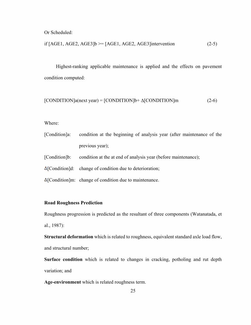
Or Scheduled:

if [AGE1, AGE2, AGE3]b >= [AGE1, AGE2, AGE3]intervention (2-5)

Highest-ranking applicable maintenance is applied and the effects on pavement

condition computed:

[CONDITION]a(next year) = [CONDITION]b+ ∆[CONDITION]m (2-6)

Where:

[Condition]a: condition at the beginning of analysis year (after maintenance of the

previous year);

[Condition]b: condition at the at end of analysis year (before maintenance);

[Condition]d: change of condition due to deterioration;

[Condition]m: change of condition due to maintenance.

Road Roughness Prediction

Roughness progression is predicted as the resultant of three components (Watanatada, et

al., 1987):

Structural deformation which is related to roughness, equivalent standard axle load flow,

and structural number;

Surface condition which is related to changes in cracking, potholing and rut depth

variation; and

Age-environment which is related roughness term.

26

QId = 13 Kgp [134 EMT (SNCK + 1)-5.0 YE4 + 0.114 (RDSb - RDSa)

+ 0.0066 CRXd + 0.42 APOTd]+ Kge 0.023 QI a (2-7)

Where:

QId: the predicted change in road roughness during the analysis year due to road

deterioration in QI;

Kgp: the user-specified deterioration factor for roughness progression (default

value= 1);

Kge: the user-specified deterioration factor for the environment-related annual

fractional increase in roughness (default value = 1);

EMT: exp (0.023 K e AGE3)

SNCK: the modified structural number adjusted for the effect of cracking, given by:

SNCK: max (1.5; SNC - SNK)

SNK: the predicted reduction in the structural number due to cracking since the last

pavement reseal, overlay or reconstruction (when the surfacing age, AGE2,

equals zero), given by:

SNK: 0.0000758 [CRX’a HSNEW + ECR HSOLD]

CRX'a: min (63; CRXa);

ECR: the predicted excess cracking beyond the amount that existed in the old

surfacing layers at the time of the last pavement reseal, overlay or

reconstruction given by:

ECR: max [min (CRXa- PCRX; 40); 0]

27

PCRX: area of previous indexed cracking in the old surfacing and base layers, given

by:

PCRX: 0.62 PCRA + 0.39 PCRW

Roughness at the end of the analysis year, before maintenance and imposing an upper limit

of 150 QI, is given by:

QIb = min (150; QIa + QId)

YAX: flow of all vehicle axles (YAX) – annual millions per lane

YE4: flow of equivalent 80 KN standard axle loads annual millions per lane

Predictions from the model are illustrated in Figure 11 for two Pavements (SNC-

values of 3 and 5) under six volumes of traffic loading and minimal maintenance

comprising the patching of all potholes (Watanatada, et al., 1987).

28

Table 1: Definitions of variables used in HDM model (Watanatada, et al., 1987)

29

Figure 10: Logic sequence of road deterioration and maintenance submodel – paved roads

(Watanatada, et al., 1987)

30

Figure 11: Prediction of roughness progression for flexible and semi – rigid pavements under

minimal maintenance of patching all the potholes (Watanatada, et al., 1987)

31

2.5 Decision making for Pavement Management

The decision making process involved in pavement management system works first with

analysing alternatives at the long term, that is, it creates possible courses of action and

examines the impact following each of them. In this regard the system is a two-tier in which

a total enumeration process creates a decision-tree-like mechanism, the second step consist

of the assessment of the consequences of each course of action by measuring its impact on

the variables of interest (i.e., condition, cost, etc.). The decision making process is guided

by a mathematical algorithm that defines the optimization problem in terms of its objectives

and constraints. The sense of the optimization is given by the nature of the objective and is

restricted by constraints which typically limit the achievement of the objective; hence,

objectives and constrains are exchangeable. In other words, an objective could be turn into

a constraint and vice versa.

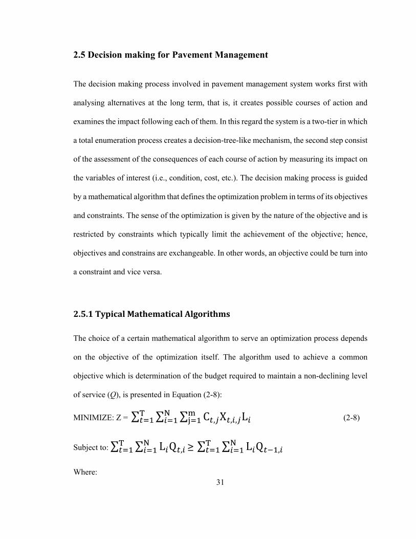
2.5.1TypicalMathematicalAlgorithms

The choice of a certain mathematical algorithm to serve an optimization process depends

on the objective of the optimization itself. The algorithm used to achieve a common

objective which is determination of the budget required to maintain a non-declining level

of service (Q), is presented in Equation (2-8):

MINIMIZE: Z = ∑ ∑ ∑ C , X , , L (2-8)

Subject to: ∑ ∑ L Q , ≥ ∑ ∑ L Q ,

Where:

32

Qt,i,j: level of service based on condition at year t, of section i, after action j

Xt,i,j: {0, 1}: 1 if treatment (j) is applied on asset (i) on time (t), zero otherwise

Li: length (size) of the asset

Ct,i,j: cost of treatment j on section i at year t

Bt: budget for year t

Another algorithm approach is used to achieve another common objective which is

determination of the budget required to achieve a target mean Level of Service (LOSn) as

presented in Equation (2-9)

MINIMIZE: Z = ∑ ∑ ∑ C , X , , L (2-9)

Subject to: ∑ ∑ L Q , ≥ (LOSn) ∑ L …..(term is fixed, constant)

Where:


LOSn: target level of service for network n (when you have more than one network of

assets)

xt,i,j: yes = 1 and no = 0;


Ct,i,j: cost of treatment j on section i at year t.

Bt: budget for year t.

33

Also, there is an algorithm to achieve a very common objective that follows the

determination of minimum budget and is that when we have a fixed budget per year (Bt)

and need to determine the best Level of Service (Q) achievable (Equation 2-10)

MAXIMIZE: Z = ∑ ∑ L , , (2-10)

Subject to: ∑ ∑ ∑ C , , , L ≤ Bt

Where:


xt,i,j: yes = 1 and no = 0;


Ct,i,j: cost of treatment j on section i at year t.

Bt: budget for year t.

2.5.2TotalEnumeration

The mathematical algorithms is supported by a total enumeration process (Watanatada, et

al., 1987) that consist of a decision-like-tree with arcs connecting paths and nodes

recording levels of service and cost per treatment option and follows a binary nature in

which a treatment may be selected or not. This enumeration process delivers expected

consequences of applying each available treatment at each segment of road at every time

step during the length of the analysis. It produces chains of alternative decision variables

from which the software selects the optimal in terms of the particular objectives and

34

constraints (Figure 12). Integer linear programming (as herein suggested) or a heuristic

method such as an evolutionary algorithm may be used to obtain a solution (although

approximate) (Imani & Amador, 2013).

Figure 12: Total enumeration process

35

CHAPTER 3

METHODOLOGY

3.1 Introduction

This chapter presents the methodology used for data acquisition and database preparation

which are necessary to develop initial pavement management system. The chapter is

divided into two main sections; the first section explains the method used to measure road

pavement roughness and presents complementary analysis to validate the proposed

approach. The second section presents the method used to prepare the database required

for the management system. The development of pavement performance curves and

treatment characterization are explained in the case study chapter for better explanation. It

is important to mention that the method herein presented aims to typify average condition

of road pavement and not to identify nor locate damage along the road pavement.

3.2 Road Roughness Measurement

Accelerometers can be used to capture vertical accelerations which are correlated to road

surface condition. Accelerometers can be found in most tablets and smart phones, they

capture accelerations in three-dimensional fashion. For the purpose of this thesis, only

vertical accelerations were of interest although the long range trend of x-accelerations

seems to map well horizontal curves and this could be used for road safety.

36

Standard deviations of accelerometer vertical accelerations captured variability or

spread around the mean of the vertical accelerations. The larger the value, the larger the

vertical accelerations. Once filtered by speed, standard deviations provided with an

estimate of pavement condition (Figure 13).

Figure 13: Standard Deviation of vertical acceleration with and without speed-normalization

3.2.1DataCollectionProtocol

There are several mobile device software applications able to log accelerations. These

applications utilize the accelerometers originally built in the mobile devices to control their

screens orientation. Few applications are able to log spatial coordinates (latitude,

longitude), speed and accelerations altogether. It is possible then to use separate

0

0.5

1

1.5

2

2.5

3

3.5

700 800 900 1000 1100 1200 1300 1400 1500

time (seconds)

Z-

Accel

era

tio

ns

Stddev_Accel_Z

Normalized_Stdev_Accel_Z

37

applications at one time to collect the desired data; i.e., one application to collect

coordinates and speed and other one to collect accelerations.

The data collection procedure herein proposed uses two sets of mobile devices and

compatible acceleration applications, as listed below:

1. Android-based device Lenovo ThinkPad with two compatible applications MyTracks

and Accelogger (MyTracks for collecting coordinates and speeds data and Accelogger

for collecting accelerations data); and

2. IOS-based devices IPad (Sometimes IPhone was used) with one compatible

application SensorLog for collecting the desired data altogether.

Data collection started at rest (zero speed) and finished at rest as well, in order to

have a known location given by a Global Positioning System (GPS). MyTracks application

required somewhere from 2 to 10 seconds to find GPS signals and triangulate the location

of the device. Lenovo ThinkPad tablet was placed horizontally on the floor of a vehicle

near the middle of it. It was a 1998 Mazda pick-up truck. For other test, various vehicles

were used to compare the acceleration observations resulting from using different dumping

systems (vehicles). This is detailed under item no. 3.2.6.

The data collection steps fall into two stages; Field Work Stage and Desk Work

Stage. The following procedure is for data collection using Lenovo device with two

applications MyTracks and Accelogger:

Field Work:

1. Start at rest and set both applications to collect data at the same time;

2. Wait for GPS signal;

38

3. Drive the vehicle non-stopping and maintain constant speed. Do not exceed 40 kph on

horizontal curves to avoid major impact of x-accelerations on z-accelerations;

4. Stop the vehicle when the traversed road surface type is changed or when 10 minutes

travel time is reached (whichever happens first). Once vehicle at rest, stop the data

collection of both applications. Data collection of any segment was stopped with

changes in surface type so that each segment contained only one type of surface. Short

changes of surface type should not be a reason to stop data collection; and

5. Register, on a field-book, date and time (beginning and end), spatial location

coordinates, surface type, qualitative appreciation of overall condition, possible

treatment type.

6. Export the collected data from the device to the computer (using email or any other

suitable mean) to the purpose of Desk Work.

Desk Work:

The data collected during the field work stage were processed to obtain the standard

deviations of the z-accelerations per second. The desk work steps are:

1. Join the collected acceleration, coordinates and speeds data;

2. Estimate the standard deviations of the vertical z-accelerations per second;

3. Estimate speeds in meter per second;

4. Normalize the standard deviations of z-accelerations by dividing them by the

corresponding speeds;

5. Multiply each normalized standard deviation by 100 to obtain the Roughness Indicators

(RIs) in one column;

39

6. Generate a column for the accumulative distance;

7. Draw a (RI-Accumulative Distance) graph; and

8. Obtain a spatial database with normalized standard deviations of z-accelerations.

Estimation of RIs of all pavements:

(Speed-normalized Standard Deviations of Vertical Accelerations)

Tool: MS Excel

Is the application able to collect the required Data

altogether?

Use Additional ApplicationNo

YESStart Data Collection

Tool: Vehicle+Tablet

Join Collected Data in One Spread Sheet

Start Data Collection

Tool: Vehicle+Tablet

Collection of Pavement Condition Data from Site1- Vertical Accelerations

2- Spatial Coordinates (Longitude + Latitude)3- Vehicle Velocities

Field Work StageData Collection

Desk Work StageStart of Database

Preparation

Figure 14: Flow chart of data collection procedure

The abovementioned procedure which was followed to collect data from site using

Lenovo set is applicable for IPad or IPhone set; however, since the latter were able to

40

collect spatial location, accelerations and speeds data altogether, there was no need to do

data join mentioned under step no. 1 of the desk work stage.

In both tablets IPad and Lenovo, the loggers took somewhere from 10 to 100

observations per second. Each road segment contained observations for a maximum of 10

minutes. It was observed that the logger took more points on rougher surfaces. For this,

one should estimate how many observations were taken in total and how many seconds

passed from start to end. Figure 14 shows the main steps of the procedure used for data

collection and processing.

3.2.2AProxyforInternationalRoughnessIndex

The Root Mean Square (RMS) is often used to capture variation on cyclical responses of

sinusoidal form. Equation (3-1) suggests that if the mean (a) is zero, the RMS equation is

equivalent to the standard deviation. Equation (3-2) shows speed-normalized RMS and

speed-normalized standard deviations of z-accelerations. As shown, such normalized-

measure captures variability on the vertical scale (z), and its units are of frequency (1/s).

N

izi

N

izi aa

nDevSta

nRMS

1

2

1

2 1..

1 (3-1)

yi

N

izzi

yi

zN

i yi

zi

yi v

aan

vv

a

nv

RMS

1

2

1

21

1 (3-2)

41

Where σz is the standard deviation of the z-accelerations (az) if the speed vyi is constant for

all observations. For this research, speed was treated as a constant because there is

corresponding speed value per observation.

A close correlation between the speed-normalized z-acceleration and the

International Roughness Index (IRI) has been suggested elsewhere (Dawkins, et al., 2011).

Values of RMS normalized by speed and multiplied by 100 could be used as proxy for IRI

(Dawkins, et al., 2011). For this research, values of speed-normalized standard deviation

of z-accelerations were equivalent to those of speed-normalized RMS, and then multiplied

by 100 to obtain a roughness index in m/km. The observed values of normalized standard

deviations are kind of 0.05, 0.04, 0.07, 0.1; so multiplying them by 100 make them similar

to the IRI values which are within a scale from 0 to 12. This doesn’t have effect on

capturing of the pavement condition, it is simply rescaling the digits to look like IRI digits.

The idea of the Roughness Indicator (RI) estimation is similar to that of International

Roughness Index (IRI), however, the RI values depend on the wheel path of the vehicle

and therefore will vary with the path followed by the driver. Also, the proposed roughness

indicator (RI) acts similarly to the International Roughness Index (IRI), lower values of RI

are associated with better condition and higher values with poorer condition.

3.2.3Normalizationbyspeed

Observed standard deviations of vertical (z-axis) accelerations were divided by

observed vehicle speed (in meter per second) to take into consideration the variability of

vehicle speed during the trip. A vehicle driver normally drives at a speed appropriate to the

42

road surface condition; i.e., if the road is in poor condition, the driver will slow down to

avoid violent movements which cause discomfort and vehicle damage. In this context,

similar values of accelerations obtained from traversing two identical hypothetical road

segments, one driven at high speed and the other one at low speed, resulted in different

values of roughness; as the standard deviations of the segment traversed with higher speed

were divided by larger speed-range and therefore delivered overall lower levels of the

condition indicator. This speed normalization process is kind of filtering the standard

deviation of vertical accelerations.

Normalization by speed (1/s) was validated using a comparison of observed values

resulted from driving a vehicle at several speeds and on different surfaces. An experiment

was set to measure vertical accelerations for three test segments at 3 speed ranges as

summarized in Table 2. Speed ranges were measured in meter per second and each value

of vertical acceleration was divided by the observed speed in meter per second.

Table 2: Target speeds (kph) for tested surfaces

Asphalt (poor condition) Gravel (fair to good) Earth (poor condition)

20 20 10

40 40 20

60 60 30

43

A comparison of speed-normalized RMS for the materials and speeds listed in Table

2 is shown on Figures 15, 16 and 17.

Figure 15: Comparison of speed-normalized standard deviation of z-accelerations – gravel – fair to

good condition – same vehicle – various speeds

Gravel Road

0

0.05

0.1

0.15

0.2

0.25

0.3

0.35

0.4

0 50 100 150 200 250 300

Distance (meters)

Sp

eed

-no

rmal

ized

StD

ev Z

40kph

20kph

60kph

44

Figure 16: Comparison of speed-normalized standard deviations of z-accelerations – asphalt – poor

condition – same vehicle – various speeds

0

0.02

0.04

0.06

0.08

0.1

0.12

0 100 200 300 400 500 600 700 800 900distancia (m)

des. est. acle‐z norm

. Vel

asf40kphasf60kphasf20kph

Asphalt Road

45

Figure 17: Comparison of speed normalized standard deviations of z-accelerations – Earth – poor

condition – same vehicle – various speeds

It should be noticed that no two trials ran over the exact same wheel path, therefore

the values of speed-normalized standard deviation of accelerations (or RMS normalized by

speed) for the same road segment are close to each other but not exactly the same. Another

reason for that is the speed effect and vehicles ability to travel over the complete vertical

irregularity. At lower speeds the vehicle is able to go all the way down and back up on a

given vertical deformation (for instance a pothole) but at higher speeds the accelerometer

is not able to register the complete vertical variation because it will travel between fewer

points of such vertical irregularity. This can be seen by comparing the vertical profiles of

gravel roads at 20, 40 and 60kph in Figure 15.

Earth Road

0

0.1

0.2

0.3

0.4

0.5

0.6

0.7

0.8

0.9

1

0 50 100 150 200

Distance (meters)

Spee

d-n

orm

aliz

ed S

tDev

. Z-a

ccel

.10kph20kph30kph

46

3.2.4ComparisonofVariousSurfaceConditions

Results showed that the use of response normalized by vehicle speed (i.e., standard

deviation normalized by speed) is capable of identifying roads at different levels of

condition (good, fair, poor) regardless of their surface material, as shown in Figure 18 for

two road segments: five and eight, S5 and S8 respectively.

Figure 18: Comparison of earth in fair- poor and asphalt in good condition

Comparison of different material segments at same levels of qualitative condition

showed similar values for the normalized response. This empirical result provides an

argument in favour of the normalization by speed. It appears that it is capable of returning

a response able to represent levels of condition (Figure 19).

Comparison Condition Poor-Good

-0.1

0.4

0.9

1.4

1.9

2.4

0 50 100 150 200 250 300 350

Time (seconds)

StD

evA

ccel

Z

Earth poor (s5)

Asphalt good (s8)

47

Figure 19: Asphalt Good-Fair condition

3.2.5ComparisonofApplicationsandDevicesUsedforDataCollection

A test of equivalency was made between the iOS's platform application SensorLog

(compatible to IPhone 4S) and Android's platform application Physics Toolbox

Accelerometer (compatible to Samsung Galaxy S4 mini). The road segment length was 275

meter and it was traversed two times in the same day. Each time for one device. Each device

was placed horizontally on the dashpool of the car which was a 2011 Toyota Corolla. The

profiles of accelerations (speed-normalized standard deviations) are shown in Figure 20.

0

0.2

0.4

0.6

0.8

1

1.2

1.4

6.7E+12 6.8E+12 6.8E+12 6.9E+12 6.9E+12 7E+12 7E+12 7.1E+12 7.1E+12

No

rmal

ized

StD

ev Z

-Acc

eler

atio

ns

GoodGood

Fair

48

The SensorLog application measures accelerations in terms of gravity acceleration

(G) that is as a percentage of 9.81m/s2 (Thomas, 2013); therefore, it was required to

multiply the acceleration readings by 9.81 m/s2. The SensorLog application collects 10

observations per second while the Physics Toolbox Accelerometer collects 15 observations

per second. As shown in Figure 20, the observations are close to each other.

Figure 20: Comparison of observations – Iphone (SensorLog) vs Samsung (Physics Toolbox

Accelerometer)

The differences between the applications observations could be explained by the

slight difference in the sensitivity of the accelerometers built in the devices, by the

difference in number of observations per second collected by each application as well as

different wheelpath traversed during the trips, because in reality there are no two trips run

over the same wheel path.

0

10

20

30

40

50

60

70

80

90

100

0 50 100 150 200 250

RI

Accumulative Distance

IOS Operation System Based Device ‐ Iphone 4S

Android Operation System Based Device ‐ Samsung Galaxy S4

49

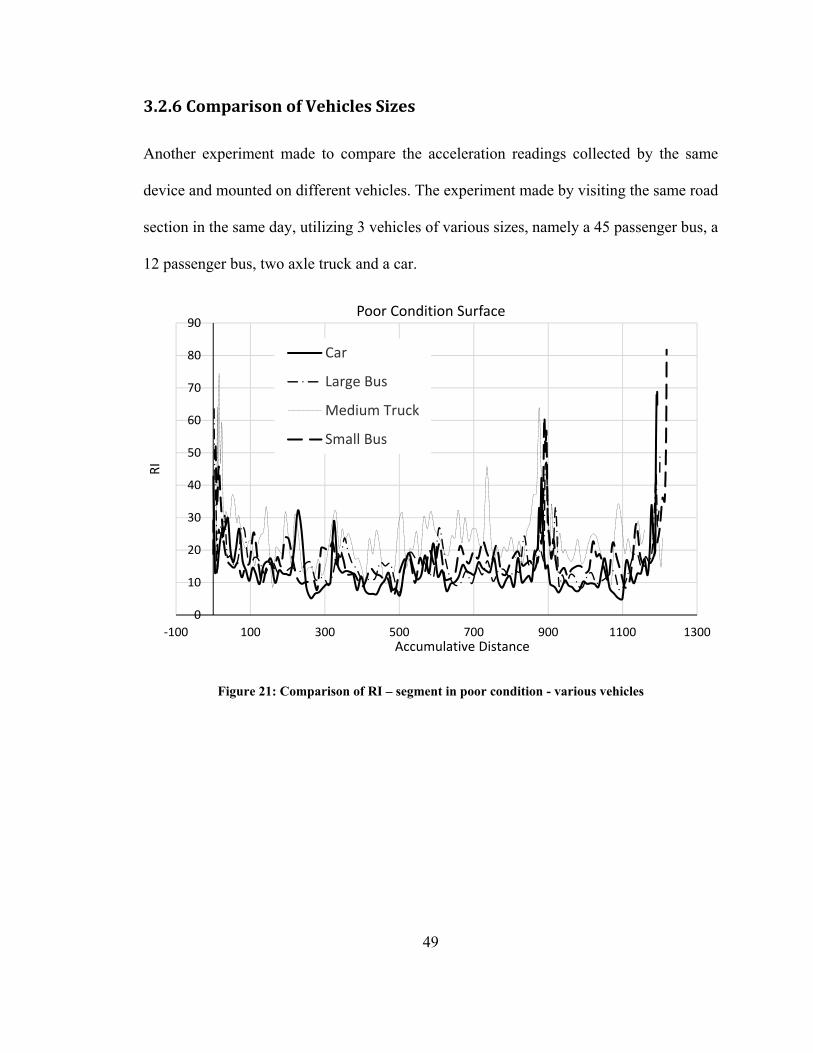
3.2.6ComparisonofVehiclesSizes

Another experiment made to compare the acceleration readings collected by the same

device and mounted on different vehicles. The experiment made by visiting the same road

section in the same day, utilizing 3 vehicles of various sizes, namely a 45 passenger bus, a

12 passenger bus, two axle truck and a car.

Figure 21: Comparison of RI – segment in poor condition - various vehicles

0

10

20

30

40

50

60

70

80

90

‐100 100 300 500 700 900 1100 1300

RI


Poor Condition Surface

Car

Large Bus

Medium Truck

Small Bus

50

Figure 22: Comparison of RI – segment in good condition – various vehicles

Vehicle size do make a difference (especially for trucks) as seen on Figures 21 and

22. It was also confirmed that initial and final observations are highly affected by the

influence of y-acceleration resulting from brake/acceleration from/to rest effects; therefore

they must be removed. At station 0+900 in Figure 21 there was a portion of heavily

deteriorated unpaved road which induced large vertical movements on the vehicles.

0

10

20

30

40

50

60

0 20 40 60 80 100 120 140 160 180 200

RI


Good Condition Surface

Small Bus

Medium Truck

Large Bus

Car

51

3.2.7ComparisonofSensorLocations

Finally, a test was made to examine the impact of device location, inside the vehicle, on

the roughness indicator. In this test, a road segment was visited three times on the same

day using the same vehicle but the IPhone was placed at different location every time. As

seen in Figure 23, it was found that the location of the instrument within the vehicle has

ignorable impact on the observed vertical accelerations.

Figure 23: Comparison of RI – same vehicle - same sensor at different locations

0

10

20

30

40

50

60

0 200 400 600 800 1000 1200

RI


Sensor in the Front Pool

Sensor in the Middle

Sensor in the Rear Pool

52

3.3 Database Preparation

The condition data collected from site, in the previous step, need to be prepared prior to its

use for developing a pavement management system. Preparing the database encompasses

several steps including extraction of the required data from the accelerometer records,

processing them and joining them (in decimal degrees WGS84) with a blank base map (in

NAD1983 CSRS). The idea of preparation phase was to obtain the average condition for

road segments of 25meters. The complete steps of database preparation are listed below

and they correspond to the case study presented in the next chapter. Also, Figure 25

illustrates the flow chart of these steps:

1. Point condition data in comma separated vector format (csv) collected from site was

processed to retain the location, speed and vertical accelerations.

2. The processed condition data was imported into ARCMAP and plotted with same

spatial reference. Each road was represented in dot format, (Figure 24).

3. The dots of each road were merged into one line. The result was linearly referenced

condition map.

4. Each road of Saint-Michelle road network was divided to segments of 25 meters.

5. Quebec roads network was imported into ARCGIS. This file is in GSC North American

1983 CSRS in decimal degrees

6. Only Saint-Michelle road network was emphasized.

7. The linearly referenced map (the 25 meters segmented map) was joined with Quebec

roads network by spatial proximity, road by road.

53

8. The RI (IRI proxy) was calculated for each segment (average value of vertical

accelerations normalized by speed and multiplied by 100.

9. Using Paterson performance model and the RI(s), the apparent age of each road

segment was calculated.

10. The final map contained database included condition data, segment length, apparent

ages and four attributes, namely, type of asset, functional classification, type of surface

and last type of intervention applied. The final map was saved as shape file and it was

the primary input for the long-term planning and optimization software (REMSOFT).

Figure 24: Point condition data-ARCGIS

54

Join the Processed Condition Data with the Road Network Map Obtained From the Agency

Tool: ArcGIS Software

1- Import condition data to ArcMap software as shp files

2- Merge all the condition shp files in one file

3- Division of each road to segments of 25 meters

4- Import main roads network into ArcMap

5- Selection of desired road network only

6- Join the condition data file resulted from step 3 with the selected local road network resulted form step 5

7- Calculate average RI of each road segment

8- Export the required attribute data to excel file

Construction of Performance Curves

Tool: Paterson Model orMunicipality Model

Calculate the Apparent Age of Each Road Segment


Merge of Apparent Ages with the Attribute Data of Step 8

Tool: MS Excel

Database is ready to Start PMS



Tool: MS Excel

Figure 25: Database preparation flow chart

55

CHAPTER 4

CASE STUDY: TOWN OF SAINT-MICHELLE

4.1 Introduction

This case study focuses on the development of initial pavement management system (PMS)

for the town of Saint Michelle, Quebec, Canada using low cost solution. Figures 26 and 27

shows town location and road network image taken by satellite, respectively. The case

study presents a novel methodology to estimate initial road surface condition in a situation

where limited budget impedes the purchase of traditional condition measurement

equipment such as Falling Weight Deflectometers (FWD) or Profilometers to estimate

International Roughness Index, which are over $125,000 in cost each. This initial condition

estimation was used to demonstrate the possibility to run a budget exercise capable of

determining long term funding needs for the allocation for maintenance and rehabilitation

of the municipal road’s pavement.

Good quality data for performance modeling is always the biggest challenge in the

implementations of initial pavement management systems that are capable of optimization

and trade-off analyses; a spatial database containing line shapefiles for the road network of

the town of Saint Michelle was assigned with condition data estimated using a vertical

accelerometer. Performance model was calibrated to indicate pavement condition across

time. Investment decisions such as what budget strategy would sustain the asset value in

the long run were performed. This decision making process required, as mentioned, the

ability to predict future asset conditions under each such investment strategy. All these

56

matters are explained in detail in this case study. Figure 28 shows flow chart of the main

work stages of the case study.

Figure 26: Location of Saint-Michelle city (Google Maps)

Figure 27: Saint-Michelle city (Google Maps)

57

Definition of Objectives and Constraints

Budget constraintNo budget constraint

Objective: Maximize the network condition regardless the budget

Example: get-rid of very poor pavements

Pre-decided budget like $ 200,000/yearNo pre-decided budget but minimize the cost

Future condition ?(< = > recent condition)

Objective: Maximize the network condition within the decided budget ($200,000/year)

Objective: Achieve certain level of network condition

Example: Status quo scenario (maintain the recent level of

condition)

ProgrammingPrinciples:

1- Stabilization, and2- Selecting the lowest cost alternative

Technique: Linear programmingTool: Remsoft software

Optimization

Technique: Enumeration + Performance CurvesTool: Solver software such as Lindo 6.2

ApprovalsBy concerned parties

Establishment of Treatment and Effectiveness Operational Window

Implementation

Figure 28: Case study main work stages

58

4.2 Construction of Saint Michelle Road Spatial Database

The first challenge was to integrate information obtained from two sources, and collected

over different spatial location systems. The first set of information were surface condition

data of 52 roads forms the road network of Saint-Michelle city. This information were

spatially referenced roughness data in point format and were collected by driving the whole

road network of the city. This condition data have been integrated with a blank base map

in line format of the same city obtained from GeoBase (GeoBase, 2013).

The method used for constructing Saint Michelle road database is indicated in the following

steps and the flow chart of Figure 29:

1. Point condition data in comma separated vector format (csv) collected from site was

processed to retain the location, speed and vertical accelerations.

2. The processed condition data was imported into ARCMAP and plotted with same

spatial reference. Each road was represented in dot format, (Figure 24).

3. The dots of each road were merged into one line. The result was linearly referenced

condition map.

4. Each road of Saint-Michelle road network was divided to segments of 25 meters.

5. Quebec roads network was imported into ARCGIS. This file is in GSC North American

1983 CSRS in decimal degrees

6. Only Saint-Michelle road network was emphasized.

7. The linearly referenced map (the 25 meters segmented map) was joined with Quebec

roads network by spatial proximity, road by road.

59

8. The RI (IRI proxy) was calculated for each segment (average value of vertical

accelerations normalized by speed and multiplied by 100.

9. Using Paterson performance model and the RI(s), the apparent age of each road

segment was calculated.

10. The final map contained database included condition data, segment length, apparent

ages and four attributes, namely, type of asset, functional classification, type of surface

and last type of intervention applied. The final map was saved as shape file and it was

the primary input for the long-term planning and optimization software (REMSOFT).

60

Join the Processed Condition Data with the Road Network Map Obtained From the Agency

Tool: ArcGIS Software

1- Import condition data to ArcMap software as shp files

2- Merge all the condition shp files in one file

3- Division of each road to segments of 25 meters

4- Import Quebec roads network map into ArcMap

5- Selection of Saint Michelle road network map only

6- Join the condition data file resulted from step 3 with the selected local road network resulted form step 5

7- Calculate average RI of each road segment

8- Export the required attribute data to excel file

Construction of Performance Curves


Calculate the Apparent Age of Each Road Segment


Merge of Apparent Ages with the Attribute Data of Step 8

Tool: MS Excel

Database is ready to Start PMS



Tool: MS Excel

Figure 29: Constructing Saint Michelle road network database – flow chart

61

4.3 Construction of Performance Curves

Strategic and long-term planning for sustainable civil infrastructure, including pavements

and other transportation systems, relies on performance prediction models. Effective

prediction of pavement performance requires adoption of the major causal contributors to

pavement deterioration which can realistically be included in the performance model.

Traffic load intensity has been recognized as the most significant factor affecting

pavements deterioration (Pedigo, et al., 1981). Also, the decision of which causal variable

to include was driven by the availability of data. Therefore, in this case study, traffic

loading was used as the primary causal factor in the performance model.

Obtaining the traffic load (ESALs) across the whole city network was limited. The

two main routes; 221 and rue Principale were assigned with Annual Average Daily Traffic

(AADT) values by Transports Qubec (TransportsQuebec, 2013) Figure 30. The rest of the

network, which are local roads, was assumed to be exposed to 35,000 ESALs over its

design life. This assumption complies with one of the methods proposed by Patterson and

Attoh-Okine back in 1992. A standard truck factor of 2.0 was assumed and percentage of

trucks was set to 10% for the sake of this academic exercise. Traffic counts should be

conducted in order to obtain a better estimate of AADT and truck percentage.

62

Figure 30: Annual Average Daily Traffic (AADT) (TransportsQuebec, 2013)

Other factors related to pavement structure such as layers thicknesses, material types

and soil strength were not available. Therefore, they were assumed to match design code

requirements.

Saint-Michelle road pavements were separated into three performance groups

depending on the traffic volumes they are exposed to. Each group was assigned different

performance curve as shown in Figure 31. These performance curves were based on a

calibrated version of modified IRI progression model developed by Paterson and Okine in

1992 (Paterson & Attoh-Okine, 1992) to match observed levels of roughness index which

varied from almost 0.4 to levels of about 160. The first performance curve was done for

Rue Principale as data for AADT levels is available (157,000 ESALs per year), m factor

for environment was set to 0.07 (Natural Resources Canada, 2013), traffic growth to 1%

63

(Statistics Canada, 2013) and thickness of pavement layers to 75mm of hot mixed asphalt

and 100mm of granular base and 150 of granular sub-base with structural coefficients of

0.22, 0.09 and 0.065 correspondingly. The second performance curve was done for the

route 221 with 350,000 ESALs per year, m equals 0.07 (Natural Resources Canada, 2013),

traffic growth to 1.5% (Statistics Canada, 2013) and thickness of pavement layers to 75mm

of hot mixed asphalt and 150mm of granular base and 150 of granular sub-base with

structural coefficients of 0.22, 0.09 and 0.065 correspondingly. The third performance

curve was done for the local roads utilizing the same method with different coefficients.

Figure 31: Pavement performance deterioration

Performance Deterioration Pavement

0

20

40

60

80

100

120

140

160

180

0 10 20 30 40 50 60

Time (years)

IRI (

m/K

m)

Local roads

principale

Route 221

64

4.4 Estimation of Intervention Treatment Type and Effectiveness

Four types of treatments were used in this model: cracksealing, microsurfacing, resurfacing

and reconstruction, corresponding to preservation, minor rehabilitation, major

rehabilitation and reconstruction for irreparable roads on the basis of one treatment per

interval of condition. Table 3 shows the cost, range of application and effectiveness of these

treatments.

Table 3: Interventions used in the analysis

Treatment

Type Cost

Operational Window Treatment

Effectiveness Lower

Boundary

Upper

Boundary

Cracksealing 0.33 $/m2 RI =< 3 3 years

Microsurfacing 6.74 $/m2 RI > 3 RI =< 6 8 years

Resurfacing 25 $/m2 RI > 6 RI =< 12 12 years

Reconstruction 42 $/m2 RI > 12 As new

65

4.5 Investment Strategies: allocation of funds and scheduling of levels of

intervention per year

Linear programming optimization was used to select the optimal combination of

interventions across time such that a given objective function is optimized and constraints

are met. The optimization procedure is performed iteratively to determine benefits

associated with each treatment, on each road element and different time (or condition)

states. The optimized schedule of works can be selected to maximize the return on

investment, while maintaining roads at an appropriate service level and considering other

constraints, such as budgets, limiting available equipment, pre-committed projects, etc. The

software used in running the linear programming in this case study was REMSOFT, a long-

term planning and optimization software. In practice, optimization of practical problems

can only be carried out using advanced software – the so-called solvers, e.g., LPABO,

LINDO, MOSEK, CPLEX, etc.

Tradeoff analysis is a complex process that tries to answer: what asset type, what

segment, what treatment should be applied and when should the road be treated over the

planning horizon so as to meet a given agency’s objective. This is done in order to compare

benefits, costs or both and determine the most effective set of strategies. Long term

investment planning (LTIP) in asset management requires trade-off of investment

strategies across variety of asset types such as bridges versus pavements, etc. The trade-off

analysis is applied to the outputs from the optimization process to select the treatment

combination (i.e., investment strategy) that will maximize the objective function. Objective

66

functions can include minimizing the cost to maintain a given road condition, maximizing

average road condition or road value over the analysis period, etc.

Deterioration curves are used to determine the optimal time to apply treatments to

roads as well as their condition after treatment application. The output from the tool is an

investment strategy that can be visualized through the map or presented as detailed tabular

reports or graphs.

Two investment strategies were analyzed. The first investment strategy evaluated is

a scenario called status quo. It is used to determine mean levels of budget required to

sustain current levels of condition across time. The second scenario looks at an

optimization that maximizes condition while restricted by budgets evolved from the budget

level obtained from the preceding scenario (status quo).

4.6 Optimization and Trade-off Analysis Results

A status quo scenario identified the need to allocate about $254,000 per year (ignoring the

final 5 years of Table 4 since scheduling of interventions falls to almost none) just to be

able to sustain current levels of condition.

It can be seen that allocation of interventions focuses on reconstructions and major

rehabilitations, following a somewhat "worst-first" approach. Even after following such

worst-first approach, still a group of segments in very poor condition remains with some

3456 (about 12%) linear meters of roads (Table 5).

67

Table 4: Annual resource allocation per intervention type

Period

Cost of

Preservation

Cost of

Rehabilitations

Cost of

Rehabilitations

Cost of

Reconstruction

Total

Cost

1 692.48 0 421,534 0 422,226

2 2,489 0 131,819 306,579 440,887

3 0 0 232,674 387,127 619,801

4 0 0 202,921 243,368 446,289

5 0 0 197,379 222,626 420,005

6 0 0 186,902 179,083 365,985

7 0 0 141,884 176,505 318,389

8 0 0 94,053 172,330 266,383

9 0 0 0 171,038 171,038

10 0 0 0 67,011 67,011

11 0 0 0 80,154 80,154

12 1,901 0 0 69,624 71,525

13 2,400 0 0 55,321 57,721

14 1,509 0 0 47,598 49,107

15 1,380 0 0 18,366 19,746

16 1,110 0 0 0 1,110

17 1,094 0 0 0 1,094

18 1,069 0 0 28.86 1,098

19 1,061 0 0 0 1,061

20 415.52 0 0 0 416

Average 254,418

Table 5: Split of roads by condition group (in linear meters)

68

Period Very Poor Condition Poor Condition Fair Condition Good Condition

0 3,581 4,659 6,543 3,300

1 4,117 3,828 5,242 4,897

2 4,839 2,768 3,483 6,993

3 5,571 1,234 2,623 8,655

4 5,692 765.69 1,613 10,013

5 5,318 621.86 990.95 11,153

6 4,988 396.52 526.41 12,173

7 4,662 399.21 0 13,022

8 4,344 52.05 0 13,688

9 4,028 52.05 0 14,003

10 3,905 52.05 0 14,127

11 3,757 52.05 0 14,275

12 3,628 52.05 0 14,403

13 3,578 0 0 14,505

14 3,490 0 0 14,593

15 3,456 0 0 14,627

16 3,456 0 0 14,627

17 3,456 0 0 14,627

18 3,456 0 0 14,627

19 3,456 0 0 14,627

20 3,456 0 0 14,627

69

The second scenario (maximization scenario) was intended to get-rid of very poor

roads and overall increase levels of condition across the network. A first attempt was done

with a $200,000 dollar per year just to find that levels of condition dropped as it was below

minimum required to sustain them obtained from the status quo scenario which is $254,418

dollar per year. A second attempt with $275,000 dollar per year showed sustain

improvement across time, however, incapable of fully eliminating very poor roads in

twenty years. Therefore, budget was raised to $350,000 per year. This latter level of budget

did resulted in full elimination of very poor roads as shown on Figure 32.

Figure 32: Progression of very poor roads across time

It is also quite interesting to note how at the beginning all segments in fair condition

are upgraded to good condition which requires a less onerous expenditure than

reconstruction broken roads, once this is achieved some money is spend to make sure good

‐1,000

0

1,000

2,000

3,000

4,000

5,000

6,000

7,000

8,000

9,000

10,000

0 1 2 3 4 5 6 7 8 9 10 11 12 13 14 15 16 17 18 19 20 21

Meters

Time (Years)

Very Poor Roads

Optimize $200,000/Year



Optimize $254,418/Year Status quo

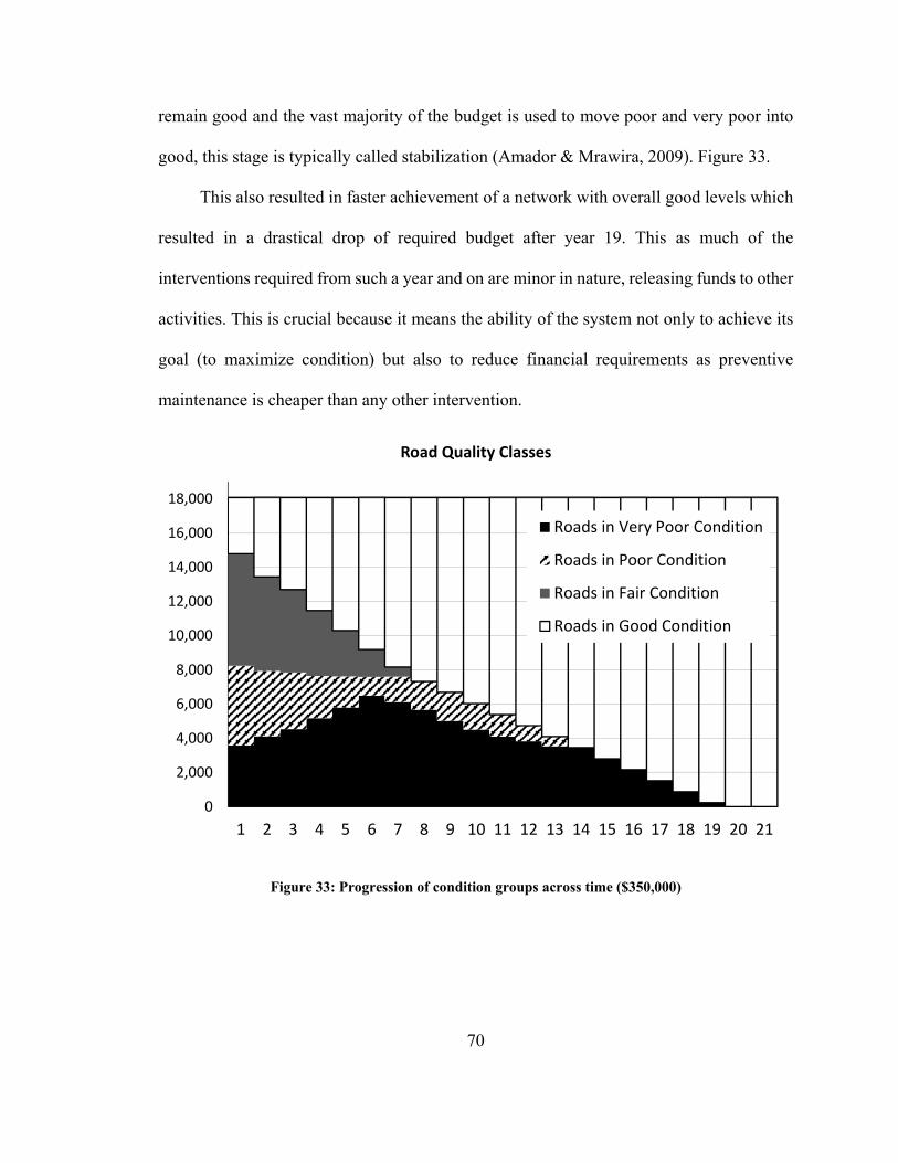
70

remain good and the vast majority of the budget is used to move poor and very poor into

good, this stage is typically called stabilization (Amador & Mrawira, 2009). Figure 33.

This also resulted in faster achievement of a network with overall good levels which

resulted in a drastical drop of required budget after year 19. This as much of the

interventions required from such a year and on are minor in nature, releasing funds to other

activities. This is crucial because it means the ability of the system not only to achieve its

goal (to maximize condition) but also to reduce financial requirements as preventive

maintenance is cheaper than any other intervention.

Figure 33: Progression of condition groups across time ($350,000)

0

2,000

4,000

6,000

8,000

10,000

12,000

14,000

16,000

18,000

1 2 3 4 5 6 7 8 9 10 11 12 13 14 15 16 17 18 19 20 21

Road Quality Classes

Roads in Very Poor Condition

Roads in Poor Condition

Roads in Fair Condition

Roads in Good Condition

71

Figure 34: Annual intervention cost ($350,000)

However, Amador and Afghari (2012) also notice a boundary effect that impedes the

solver to realize of the impact of the decisions on the long term when there is no long term,

this has been also found in economics of overlapping generations. Therefore results from

two years before the end of the 20 year period can be seen as a 2 year optimization and

those of the final year as isolated annual optimization. A somewhat lazy allocation of

treatments can be observed at the beginning, no explanation can be provided on this regard.

0

50,000

100,000

150,000

200,000

250,000

300,000

350,000

1 2 3 4 5 6 7 8 9 10 11 12 13 14 15 16 17 18 19 20

Intervention Costs (CAN$)

Cost of Preserve

Cost of Minor Rehabilitation

Cost of Major Rehabilitation

Cost of Reconstruction

72

Figure 35: Time progression of mean network condition ($350,000)

0

2

4

6

8

10

12

14

16

0 1 2 3 4 5 6 7 8 9 10 11 12 13 14 15 16 17 18 19 20 21

IRI

Time (years)

Network Condition

Average IRI

73

CHAPTER 5

CONCLUSIONS AND RECOMMENDATIONS

5.1 Conclusions

This thesis presents a low cost method to measure pavement surface condition based on

roughness and utilize it in developing initial pavement management system. In particular

it shows the capability of using the accelerometer built in a tablet or smart phone to capture

surface vertical irregularities and condense them into an indicator of condition. This

indicator was utilized in the development of initial pavement management system.

This method is expected to help municipalities and governments in developing

countries which lack financial resources to purchase expensive equipment to quickly assess

the condition of their network and implement a pavement management system. This system

is capable of allocating resources in a way that condition across the network is sustained at

good levels and public funds are invested in a cost-effective manner. It does so by looking

at the impact of long term strategies of sustain funding and their use on preservation, minor

and major rehabilitation interventions.

A case study of a small municipality (the city of Saint Michelle in the suburb of

Montreal, Quebec) was used to demonstrate how this condition indicator which is resulted

from the low-cost road surface condition measurement paved the way for the

implementation on an initial pavement management system. Performance curves were

produced on the basis of expert criteria and empirical method used by the World Bank

(Paterson & Attoh-Okine, 1992)(Watanatada, et al., 1987). A decision making system was

74

used to find out required levels of annual funding to sustain good levels of condition across

time.

A fully optimized investment strategy based on network-wide average roughness

index was able to restore the whole network in good condition (IRI lesser than 1.8) after

18 years and also eliminate very poor, poor and fair roads. These findings are consistent to

many studies (Abaza, et al., 2004) (Abaza, 2006) on pavement preservation best practice –

demonstrating that spending money on the good roads first (“keep good roads good”) is

the most efficient way of managing roads.

In numbers’ language, the investment scenarios showed the need to have at least

$254,418 per year to sustain current levels of condition. A larger budget of $275,000 per

year was required to achieve improvement. An even larger budget of about $350,000 per

year was required to recover the entire network and move it into good levels of condition.

Moreover, the required levels of funding dropped after year 18, showing that only

preservation and minor rehabilitation activities, which are much cheaper than major

rehabilitation and reconstruction, were required.

The effect of reducing the budget to $275,000 per year on the optimized program of

works is that it will take longer time to achieve a network average roughen index of less

than 1.8. In this case, it will take more than 20 years, and yet some roads will remain at

very poor condition.

75

5.2 Recommendations

Future research needs to look into filtering algorithms to clean the collected data in order

to remove the effect of undesirable features (per instance speed reducer bumps).

Operational windows for treatment application should be matched with local

experience; hence, a group of roads already scheduled to receive dissimilar levels of

intervention should be visited in order to learn from local circumstances the range of

variation in condition to which specific treatments are allocated.

It is also advisable to measure levels of condition after treatment application in order

to estimate treatment effectiveness jump. Intervened roads should be visited annually in

order to develop a database of after treatment performance. Non-intervened roads should

also be visited in order to estimate deterioration rates and develop deterioration models

adjusted to local circumstances. Also, traffic loading should be based on traffic counts and

weight estimation for the municipal roads.

All this information should be used in order to update and improve the model such

that it is truly calibrated to local circumstances. Finally it should not be forgotten the fact

that current interventions as applied for certain circumstances does not rule out other

applicable treatments as technology evolves that could be more effective, also the quality

of local contractors is not necessarily the best. All this can be estimated by measuring the

before and after trends at intervened pavements.

76

REFERENCES

Abaza, K. A., 2006. Iterative Linear Approach for Nonlinear Nonhomogeneous Stochastic

Pavement Management Models. Journal of Transportation Engineering, Vol. 132,

American Society of Civil Engineering, pp. 244-256.

Abaza, K. A., Ashur, S. A. & Al-Khatib, I. A., 2004. Integrated Pavement Management

System with a Markovian Prediction Model. Journal of Transportation Engineering,

Vol. 130, American Society of Civil Engineering, pp. 24-33.

Amador, L. & Afghari, A., 2012. Lifecycle Optimization and Tradeoff Analysis among

Competing Objectives for a Road Corridor. s.l., Transportation Research Board

Annual Meeting 2012 Paper #12-0342.

Amador, L. & Magnuson, S., 2011. Adjacency Modeling for Coordination of Investments

in Infrastructure Asset Management-Case Study of Kindersley, Saskatchewan,

Canada. Transportation Research Record: Journal of the Transportation Research

Board of the National Academies, No. 2246, Washington, D.C., pp. 8-15.

Amador, L. & Mrawira, D., 2009. Roads Performance Modeling and Management System

from two condition data points: Case study of Costa Rica. Journal of Transportation

Engineering, ASCE Vol 135, No.12, pp. 999-1007.

Amador, L. & Mrawira, D., 2011. Capturing Variability in Pavement Performance Models

from Sufficient Time-Series Predictors: A Case Study of the New Brunswick Road

Network. Canadian Journal of Civil Engineering , Volume 38, pp. 210-220.

Archondo, R., 1999. Typical Unpaved Roads Roughness Predicted By the HDM-III Model.

Infrastructure Notes - The World Bank, Volume Transport No. RT-1, pp. 1-5.

77

Bennett, C., 1996. Calibrating Road Roughness Meters in Developing Countries.

Transportation Research Record: Journal of the Transportation Research Board of

the National Academies, No. 1536, Washington, D.C., pp. 73-81.

Butler, Z., 2013. Advanced Paving Solutions. [Online] Available at:

http://www.advancedpavingsolutions.com/commonproblems/ [Accessed 9 October

2013].

Capuruco, R., Hegazy, T., Tighe, S. & Zaghloul, S., 2005. Full-Car Roughness Index as

Summary Roughness Statistic. Transportation Research Record: Journal of the

Transportation Research Board of the National Academies, No. 1905, Washington,

D.C., pp. 148-156.

Chen, X., Hudson, S., Pajoh, M. & Dickinson, W., 1996. Development of New Network

Optimization Model for Oklahoma Department of Transportation. Transportation

Research Record: Journal of the Transportation Research Board of the National

Academies, No. 1524, Washington, D.C., pp. 103-108.

Dawkins, J., Bevly, D., Powell, B. & Bishop, R., 2011. IntelliDrive Pavement Maintenance

Application Quarterly Report, s.l.: s.n.

Delanne, Y. & Pereira, P., 2001. Advantages and Limits of Different Road Roughness

Profile Signal-Processing Procedure Applied in Europe. Transportation Research

Record: Journal of the Transportation Research Board of the National Academies,

No. 1764, Washington, D.C., pp. 254-259.

Dore, G. & Zubeck, H. K., 2009. Cold Regions Pavement Engineering. U.S.A.: American

Society of Civil Engineers (ASCE).

78

Falls, L. C., Hass, R., McNeil, S. & Tighe, S., 2001. Asset Management and Pavement

Management Using Common Elements to Maximize Overall Benefits.

Transportation Research Record: Journal of the Transportation Research Board of

the National Academies, No. 1769, Washington, D.C., pp. 1-10.

FHWA & AASHTO, 1997. Asset Management: Advancing the State of the Art into the

21st Century Through Public-Private Dialogue. Transportation Research Record:

Journal of the Transportation Research Board of the National Academies, No.

FHWA-RD-97-046, Washington, D.C., p. 16.

GeoBase, 2013. GeoBase. [Online] Available at:

http://www.geobase.ca/geobase/en/search.do?produit=nrn&language=en

[Accessed 2 August 2013].

George, K. P., Rajagopal, A. S. & Lim, L. K., 1989. Models for Predicting Pavement

Deterioration. Transportation Research Record: Journal of the Transportation

Research Board of the National Academies, No. 1215, Washington, D.C., pp. 1-7.

Guignard, J. C., 1971. Human Sensitivity to Vibration. Journal of Sound and Vibration,

Vol. 15, pp. 11-16.

Haas, R., Hudson , R. & Zaniewski , J., 1994. Modern Pavement Management. FL: Krieger

Publishing Comany.

Hall, K. & Munoz, C., 1999. Estimation of Present Serviceability Index from International

Roughness Index. Transportation Research Record: Journal of the Transportation

Research Board of the National Academies, No. 1655, Washington, D.C., pp. 93-99.

Huang, Y. H. & Mahboub, K., 2004. Pavement Analysis and Design. 2nd ed. U.S.A.:

Pearson Education, Inc..

79

Hudson, W. R., Uddin, W. & Hass, R. C., 1997. Infrastructure Management. New York:

McGraw-Hill.

Imani, A. F. & Amador, L., 2013. Towards A Sustainable Pavement Management:

Incorporating Environmental Impacts of Pavement Treatments Into A Performance-

Based Optimization. Washington D.C., Transportation Research Board-92nd Annual

Meeting.

Khan, R., Helali, K., Jumikis, A. & He, Z., 2003. Deficiency Analysis of As-Built Database

to Enhance a Pavement Management System. Transportation Research Record:

Journal of the Transportation Research Board of the National Academies, No. 1853,

Washington, D.C., pp. 55-64.

Ksaibati, K., McNamara, R., Miley, W. & Armaghani, J., 1999. Pavement Roughness Data

Collection and Utilization. Transportation Research Record: Journal of the


D.C., pp. 86-92.

Litzka, J. et al., 2008. The Way Forward for Pavement Performance Indicators Across

Europe - COST Action 354 Performance Indicators for Road Pavements - Final

Report, s.l.: European COoperation in the field of Scientific and Technical Research.

Mactutis, J., Alavi, S. & Ott, W., 2000. Investigation of Relationship Between Roughness

and Pavement Surface Distress Based on WesTrack Project. Transportation



Mallick, R. B. & El-Korchi, T., 2013. Pavement Engineering. USA: CRC Press, Taylor &

Francis Group.

80

Mannering, F. L., Washburn, S. S. & Kilareski, W. P., 2009. Principles of Highway

Engineering and Traffic Analysis. 4th ed. U.S.A.: John Wiley & Sons, Inc..

Natural Resources Canada, 2013. Natural Resources Canada. [Online]

Available at: http://geogratis.gc.ca/api/en/nrcan-rncan/ess-sst/0f7e60fd-c3c4-595a-

8f8e-679c6c2c65d9.html [Accessed 12 August 2013].

Noureldin, S., Zhu, K., Li, S. & Harris, D., 2003. Network Pavement Evaluation with

Falling-Weight Deflectometer and Ground-Penetrating Radar. Transportation



Papagiannakis, A. T. & Masad, E. A., 2008. Pavement Design and Materials. New Jersey:

John Wiley and Sons, Inc..

Paterson, W. D. & Attoh-Okine, B., 1992. Simplified Models of Paved Road Deterioration

Based on HDM-III. s.l., Transportation Research Board.

Pavemanpro.com, 2013. pavemanpro. [Online] Available at:

http://www.pavemanpro.com/article/identifying_asphalt_pavement_defects/

[Accessed 8 October 2013].

Pavementinteractive, 2013. Pavement Interactive. [Online] Available at:

http://www.pavementinteractive.org/article/rutting/ [Accessed 7 October 2013].

Pedigo, D., Hudson, R. & Roberts, F., 1981. Pavement Performance Modeling for

Pavement Management. Transportation Research Record: Journal of the


D.C., pp. 14-21.

81

Posavljak, M., Tighe, S. & Godin, J., 2013. Strategic Total Highway Asset Management

Integration (STHAMi). Washington, D.C., Transportation Research Board 92nd

Annual Conference.

Prozzi, J. A. & Madanat, S. M., 2003. Incremental Nonlinear Model for Predicting

Pavement Serviceability. Journal of Transportation Engineering, Vol. 129,

American Society of Civil Engineering, pp. 635-641.

Roadex, 2013. Roadex Network. [Online] Available at:

http://www.roadex.org/index.php/permanent4#4.1.5 [Accessed 6 November

2013].

Roberts, F. L. et al., 1996. Hot Mix Asphalt Materials, Mixture, Design and Constructio.

2nd ed. Lanham, Md: Natinal Asphalt Pavement Association Research and

Education Foundation.

Sayers, M. W., 1995. On the Calculation of International Roughness Index from

Longitudinal Road Profile. Transportation Research Record: Journal of the


D.C., pp. 1-12.

Sayers, M. W. & Karamihas, S. M., 1998. The Little Book of Profiling-Basic information

About Measuring and Interpreting Road Profiles. Michigan: University of

Michigan-Transportation Research Institute (UMTRI) .

Statistics Canada, 2013. Statistics Canada. [Online] Available at:

http://www.statcan.gc.ca/daily-quotidien/130926/t130926a002-eng.htm [Accessed

8 November 2013].

82

TAC, 1977. Pavement Management Guide. Ottawa: Transportation Association of Canada

(TAC).

TAC, 1997. Pavement Design and Management Guide. Ottawa: Transportation

Association of Canada (TAC).

TAC, 1999. Highway Asset Management Systems: a primer. s.l.:Transportation

Association of Canada (TAC).

Takayama, S., 2013. [Online] Available at:

https://play.google.com/store/apps/details?id=jp.daikiko.Accelogger&hl=en

[Accessed 2 June 2013].

Tarpay, M., Tapio, R. & Talvitie, A., 1996. Using a Pvement Management System for

Allocating Resources: Case Study of Hungary. Transportation Research Record:

Journal of the Transportation Research Board of the National Academies, No.

1518, Washington, D.C., pp. 78-84.

Thomas, B., 2013. Apple. [Online] Available at:

https://itunes.apple.com/ca/app/sensorlog/id388014573?mt=8 [Accessed 2 June

2013].

Thom, N., 2008. Principles of Pavement Engineering. London: Thomas Telford

Publishing.

TransportsQuebec, 2013. ATLAS des transports quebec. [Online] Available at:

http://transports.atlas.gouv.qc.ca/Infrastructures/InfrastructuresRoutier.asp

[Accessed 2 August 2013].

UDOT, 2009. Pavement Preservation Manual - Part 2 - Pavement Condition Data, s.l.:

Utah Department of Transportation (UDOT).

83

WAPA, 2013. Washington Asphalt Pavement Association (WAPA). [Online]

Available at: http://www.asphaltwa.com/2010/09/18/transverse-thermal-cracking/

[Accessed 8 December 2013].

Watanatada, T. et al., 1987. The Highway Design and Maintenance Standards Model -

HDM III. Washington D.C.: Word Bank - John Hopkins University.

Documents

A Low Cost Method to Develop an Initial Pavement ... · I A Low Cost Method to Develop an Initial Pavement Management System A Thesis in The Department of Building, Civil and Environmental