UNIVERSITÉ DE GENÈVE FACULTÉ DES SCIENCES Département de Chimie Minérale, Professeur J. Buffle Analytique et Appliquée Département d’Informatique Professeur B. Chopard Département de Chimie - Université de Lleida Professeur J. Galceran

A Lattice Boltzmann numerical approach for modelling reaction-diffusion processes in chemically and physically heterogeneous

environments

THÈSE

présenté à la Faculté des sciences de l’Université de Genève pour obtenir le grade de Docteur ès sciences, mention interdisciplinaire

par

Davide Alemani

de

Corbetta (Italie)

Thèse No Sc. 3850

GENÈVE

2007

Contents

Acknowledgements vii

Résumé de la thèse (in French) ix

1 Introduction 11.1 Motivation . . . . . . . . . . . . . . . . . . . . . . . . . . . . . 11.2 Environmental Processes . . . . . . . . . . . . . . . . . . . . . 2

1.2.1 Chemically heterogeneous systems . . . . . . . . . . . . 21.2.2 Physicochemical complex geometry: Biofilm . . . . . . 4

1.3 The method proposed . . . . . . . . . . . . . . . . . . . . . . 51.4 Organisation of the thesis . . . . . . . . . . . . . . . . . . . . 61.5 Publications . . . . . . . . . . . . . . . . . . . . . . . . . . . . 7

I The model and Validation 9

2 The Physical Problem 112.1 Overview . . . . . . . . . . . . . . . . . . . . . . . . . . . . . . 112.2 The Problem . . . . . . . . . . . . . . . . . . . . . . . . . . . 11

2.2.1 The prototype problem . . . . . . . . . . . . . . . . . . 122.2.2 Space scales: Diffusion and reaction layer thicknesses . 152.2.3 Diffusion and reaction time scales . . . . . . . . . . . . 16

2.3 A typical Multi-scale problem . . . . . . . . . . . . . . . . . . 172.4 The mathematical formulation of the problem for Multiligand

applications . . . . . . . . . . . . . . . . . . . . . . . . . . . . 192.4.1 Reaction-Diffusion equations . . . . . . . . . . . . . . . 192.4.2 Initial Conditions . . . . . . . . . . . . . . . . . . . . . 212.4.3 Boundary Conditions . . . . . . . . . . . . . . . . . . . 21

2.5 Summary . . . . . . . . . . . . . . . . . . . . . . . . . . . . . 23

i

3 The Lattice Boltzmann Method for Reaction-Diffusion Pro-cesses 253.1 Overview . . . . . . . . . . . . . . . . . . . . . . . . . . . . . . 253.2 The Lattice Boltzmann Approach . . . . . . . . . . . . . . . . 253.3 The Lattice Boltzmann Reaction-Diffusion Model . . . . . . . 27

3.3.1 General description . . . . . . . . . . . . . . . . . . . . 273.3.2 A way to compute the flux . . . . . . . . . . . . . . . . 303.3.3 The regularised LBGK method for reaction-diffusion

problem . . . . . . . . . . . . . . . . . . . . . . . . . . 313.4 A convergence analysis of LB methods for the prototype reaction 32

3.4.1 Pure diffusive case . . . . . . . . . . . . . . . . . . . . 333.4.2 Pure reactive case . . . . . . . . . . . . . . . . . . . . . 343.4.3 Reactive-Diffusive case . . . . . . . . . . . . . . . . . . 353.4.4 Comparison of convergence conditions between Stan-

dard and Regularised schemes . . . . . . . . . . . . . . 363.5 The numerical initial and boundary conditions . . . . . . . . . 393.6 Summary . . . . . . . . . . . . . . . . . . . . . . . . . . . . . 43

4 The Multi-scale Methods: Time Splitting and Grid Refine-ment 454.1 Overview . . . . . . . . . . . . . . . . . . . . . . . . . . . . . . 454.2 The Time splitting Method . . . . . . . . . . . . . . . . . . . 46

4.2.1 Introduction . . . . . . . . . . . . . . . . . . . . . . . . 464.2.2 The basics of the time splitting method . . . . . . . . . 474.2.3 The time splitting method in the LBGK framework . . 484.2.4 Time splitting validation . . . . . . . . . . . . . . . . . 51

4.3 The Grid Refinement Methods . . . . . . . . . . . . . . . . . . 564.3.1 The reason to refine the grid . . . . . . . . . . . . . . . 564.3.2 The grid refinement schemes . . . . . . . . . . . . . . . 574.3.3 Grid refinement validation . . . . . . . . . . . . . . . . 614.3.4 Good choice of grid parameters for a typical reactive

systems. . . . . . . . . . . . . . . . . . . . . . . . . . . 644.4 The complete numerical scheme . . . . . . . . . . . . . . . . . 68

4.4.1 The numerical algorithm . . . . . . . . . . . . . . . . . 684.4.2 The complete scheme for the prototype problem . . . . 69

4.5 Summary . . . . . . . . . . . . . . . . . . . . . . . . . . . . . 72

II 1D systems.Multiligand and Chemically Heterogeneous Systems.

ii

Program validation and applications. 73

5 Chemical validation and some studies of simple multiligandsystems 755.1 Overview . . . . . . . . . . . . . . . . . . . . . . . . . . . . . . 755.2 Validation with a system of electrochemical interest . . . . . . 75

5.2.1 Simulation of voltammetric curves . . . . . . . . . . . . 755.2.2 Validity of the numerical model in excess of ligand . . . 76

5.3 Some studies with simple multiligand systems . . . . . . . . . 805.3.1 Mixture of ligands in excess compare to metal . . . . . 805.3.2 Computation of flux without ligand excess . . . . . . . 835.3.3 Mixture of complexes; the use of several grids . . . . . 84

6 Fluxes in environmental Multiligand systems 896.1 Overview . . . . . . . . . . . . . . . . . . . . . . . . . . . . . . 896.2 A summary of the physical model and boundary and initial

conditions . . . . . . . . . . . . . . . . . . . . . . . . . . . . . 906.3 Metal fluxes in presence of simple Ligands: OH− and CO2−

3 . . 936.3.1 Metal complex distribution and simulation conditions . 936.3.2 Results at constant [CO2−

3 ]tot and varying pH . . . . . 956.3.3 Results at constant pH and variable [CO2−

3 ]tot . . . . . 976.4 Metal fluxes in presence of Fulvic Acids . . . . . . . . . . . . . 98

6.4.1 Simulation conditions . . . . . . . . . . . . . . . . . . . 986.4.2 Time evolution of total flux and concentration profiles 1046.4.3 Distribution of individual fluxes and lability degree, at

steady-state . . . . . . . . . . . . . . . . . . . . . . . . 1046.5 Metal fluxes in presence of suspended particles/aggregates . . 111

6.5.1 Simulation conditions . . . . . . . . . . . . . . . . . . . 1116.5.2 Simulation results . . . . . . . . . . . . . . . . . . . . . 114

6.6 Metal fluxes in mixtures of environmental complexants . . . . 1176.7 Computational time: performance of MHEDYN . . . . . . . . 1216.8 Summary . . . . . . . . . . . . . . . . . . . . . . . . . . . . . 122

III 3D systems.Physicochemical Validation and an Environmental Ap-plication 123

7 Physicochemical validation 1257.1 Overview . . . . . . . . . . . . . . . . . . . . . . . . . . . . . . 125

iii

7.2 3D case: comparison of LBGK performance without and withgrid refinement . . . . . . . . . . . . . . . . . . . . . . . . . . 1257.2.1 Case of inert complex in 3D . . . . . . . . . . . . . . . 1267.2.2 Semi-labile complex in 3D at a spherical electrode . . . 1287.2.3 Gain of computation time in 3D with grid refinement . 129

7.3 AGNES simulation . . . . . . . . . . . . . . . . . . . . . . . . 1307.4 Summary . . . . . . . . . . . . . . . . . . . . . . . . . . . . . 133

8 Modeling Fluxes in a Biofilm 1358.1 Overview . . . . . . . . . . . . . . . . . . . . . . . . . . . . . . 1358.2 General description of a Biofilm . . . . . . . . . . . . . . . . . 1358.3 A biofilm model . . . . . . . . . . . . . . . . . . . . . . . . . . 1368.4 The numerical method: BIODYN . . . . . . . . . . . . . . . . 137

8.4.1 The method . . . . . . . . . . . . . . . . . . . . . . . . 1378.4.2 The condition at 3D - 1D interface . . . . . . . . . . . 1418.4.3 parallelisation of the code . . . . . . . . . . . . . . . . 142

8.5 Metal fluxes in presence of the reaction M­ML at differentlability . . . . . . . . . . . . . . . . . . . . . . . . . . . . . . . 1448.5.1 Simulation conditions . . . . . . . . . . . . . . . . . . . 1448.5.2 Simulation results . . . . . . . . . . . . . . . . . . . . . 145

8.6 Summary . . . . . . . . . . . . . . . . . . . . . . . . . . . . . 152

9 Conclusions and Perspectives 1539.1 Contributions . . . . . . . . . . . . . . . . . . . . . . . . . . . 1539.2 Perspectives . . . . . . . . . . . . . . . . . . . . . . . . . . . . 155

Bibliography 157

Appendices 168

A The derivation of the reaction-diffusion equation from theLattice Boltzmann equation 169A.1 Setting up the scene . . . . . . . . . . . . . . . . . . . . . . . 169A.2 The Chapman-Enskog procedure . . . . . . . . . . . . . . . . 170

B Convergent criteria: the spectral radius and the Banach The-orem 175

C Lability degree at steady-state for multiligand systems 177

D List of parameters of simple ligand simulations 179

iv

E List of parameters of Fulvic Acids simulations 191

F List of parameters of Particles/Aggregates simulations 209

G List of parameters of mixture simulations 217

v

Acknowledgements

During my PhD years in Geneva, I have had the pleasure of meeting a lotof different people. They come from many different countries, with differentcultures and of different extractions. I learnt something from each of themwhich has helped me to be tolerant and respectful of the differences in people.I would like to thank my advisor, Jacques Buffle for his trust and confidencein me for all these years. He has coached and lead me to the concepts ofthe environmental chemistry. Thank you to my co-advisor, Bastien Chopardwhose fruitful suggestions always gave me the right direction to take and tohave introduced me to the Lattice Boltzmann Method. Thank you to myco-advisor, Joseph Galceran for being always close to me and for having ded-icated to me a lot of his time. I am grateful for all the discussions we had inthe Campus of Lleida on the chemical complexation of a metal and on thebeauty of the land and the idiom of Catalunya.Thank you to Serge Stoll, Jaume Puy and William Davison who have ac-cepted to be in the jury of my thesis’s defense.I like to remember my lecturer and mentor at the department of Physics inMilano, Fausto Valz-Gris. I am enormously grateful to him for his preciousteachings.Thank you to my colleagues at the University and to all the friends whomI have met in Geneva and beyond. Thank you to Tatiana Pieloni, FedericoKaragulian, Silvia Diez, Paolo Galletto, Andrea Vaccaro, Paul Albuquerque,Andrea Parmigiani, Hung Phi N’Guyen, Fokko Beekhof, Vincent Keller,Jonas Latt, Berhnard Sonderegger, Rafik Ouared, Jean-Luc Falcone, KimJee Hyub, Sandra Salinas, Zeshi Zhang, Andrea Marconetti, Ivan Sartini,Jonh Mendez, Emilio Sanchez, Lucia Niola, Paola Lezza and to those friendswhich I have absent mindedly forgotten to mentioned today.Special thanks to Marco Cattaneo, for his friendship and for all the Ferragostowe spent together and for those we did not spend. To Andrea Vaccaro,I would like to thank him for his friendship and support especially duringthose challenging times when I was writing my thesis.In particolare, grazie di cuore alla mia famiglia, per avere creduto in me e

vii

per avermi permesso di studiare e seguire la mia strada, senza interferire mai,dandomi sempre i mezzi per continuare e innumerevoli e preziosi consigli. Amia mamma e mio papà devo tutto. Grazie al mio fratellino, Andrea checon mia grande soddisfazione sta studiando matematica. Huge thanks to myfamily.Last but not least, a warm thank you to my lovely fiancée Mena, for beingunderstanding, supportive and most of all, patient. Thank you for her loveand her incredible grace in being with me. Her love and her smile will con-tinue to make me the happiest man in the world.

Once again, thank you to all.

viii

Résumé de la thèse

Introduction à la problématique

Cette thèse propose une nouvelle méthode numérique de solution des prob-lèmes de reaction-diffusion dans les milieux environnementaux, comme lessystèmes aquatiques, le milieu poreux, les sédiments, les sols et les biofilms.En particulier, la thèse étude les processus liés à la complexation d’un métaldans les milieu aquatiques et les biofilms. Dans ces systèmes les valeursdes constantes de vitesse, des coefficients des diffusions et des constantsd’équilibre, peuvent varier sur des de nombreux ordres de grandeur en fonc-tionne de la nature des ligands chimiques et de la structure physique dumilieu.Avec la croissance de la puissance des ordinateurs, en termes de mémoire etde vitesse de calculs, la modélisation numérique est devenue un outil de plusen plus essentiel pour simuler la grand variété des processus naturels.Le but de cette thèse est de développer un nouvel algorithme numérique basésur la méthode de réseau de Boltzmann (Lattice Boltzmann Method).Le modèle développé dans cette thèse considère deux processus de base: ladiffusion et la réaction chimique. Le problème général étudié dans cette thèseréside dans le fait qu’un très grand nombre d’équations de reaction-diffusiondoit être traité pour un même métal M, dans une solution chimique qui con-tiens un grand nombre de ligands et de complexes. En particulier, l’objectifspécifique est de calculer le flux du métal M sur une surface où il est con-sommé, comme sur les senseurs bioanalogiques et les micro-organismes, etd’étudier l’impact des différents complexes formés dans les systèmes environ-nementaux.En particulier, cette thèse propose deux codes numériques, provenant dumême algorithme:

1. MHEDYN - Pour calculer le flux d’un métal M sur une surface plaineoù M est consommé, dans le cas de systèmes environnementaux chim-iquement hétérogènes mais physiquement homogènes.

ix

Figure 1: Diagramme schématique des processus physico-chimiques qui ont lieuproche d’une interface où l’ion métallique est consommé, soit une électrode ou unemicro-organisme.

2. BIODYN - Pour calculer le flux d’un métal M en présence d’un lig-and L dans des modèles de biofilms en 3D, c’est à dire des systèmesphysiquement hétérogènes.

Le problème physique

Le problème physico-chimique est résumé de manière schématique dans lafigure 1. Dans cette thèse on a concentré notre étude sur les phénomènesde consommation (uptake) d’un ion métallique (tel que Cu2+, Zn2+, Al2+

. . . ) à une interface en relation avec la complexation du métal par les ligandsenvironnementaux.Les ligands naturels sont classifiés en trois groupes:

1. Ligands simples organiques et inorganiques, tel que OH−, CO2−3 , les

acides aminés ou l’oxalate. On peut les trouver souvent en fort excèspar apport aux métaux de transition et aux métaux de type b

2. Les bio-polymères organiques, dont les plus importants sont les acidesfulvics

3. Les particules et les agrégats de particules dans le domaine de taillede 1-1000 nm. La majorité des agrégats est composé par solides in-organiques tels que des oxydes métalliques (argiles, oxydes de fer . . .).

x

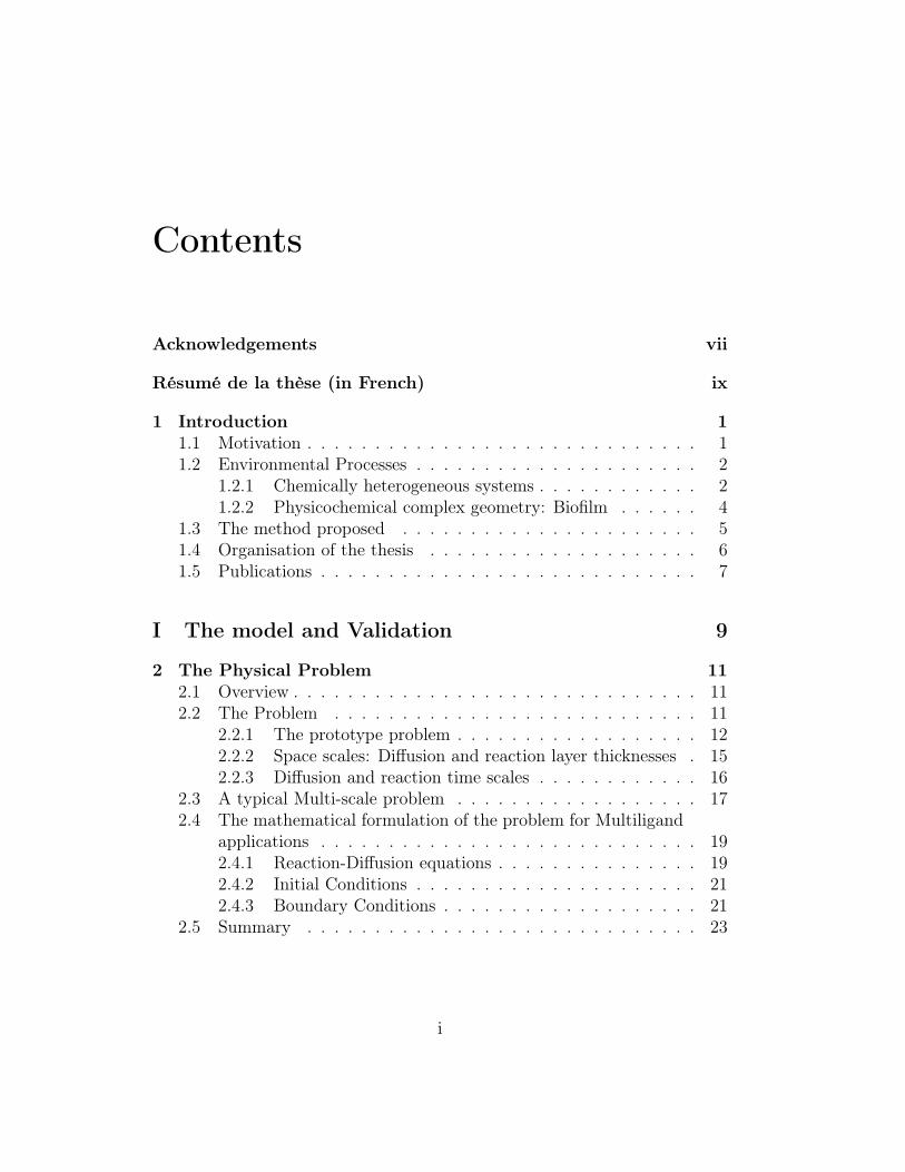
Concentrations du Métal10−8 mol m−3 – 10−3 mol m−3

Coefficients de diffusions10−13 m2 s−1 – 10−9 m2 s−1

Constantes de vitesse de réactions10−6 s−1 – 109 s−1

Table 1: Domaine de valeurs des plus importants paramètres physico-chimiquesdans les milieu environnementaux

La difficulté principale est lié à la nécessité de prendre en considéra-tion toutes les interactions conformationelles électrostatique et covalententre les métaux et ces ligands.

Les ligands environnementaux présentés ci-dessus peuvent être décrits parune ensemble de réactions chimiques de première ordre, de la forme:

M + Lkd

®

ka

ML

où kd et ka sont les constantes de vitesse de dissociation et d’association dela réaction. En outre, toutes les espèces chimiques diffusent en solution avecleur coefficient de diffusion. Les domaines typiques des concentration desions métalliques, des constantes d’association chimique et des coefficients dediffusion dans les milieu environnementaux sont résumés dans le tableau 1.La caractéristique important qu’il faut souligner et dont il faut tenir comptepour une simulation numérique correcte, est que ces valeurs varient sur denombreux ordres des grandeur. Pour cette raison on proposera deux méth-odes multi-echelles, le time splitting et le raffinement de grille.Dans le chapitre 2 on décrit les équations chimiques et mathématiques com-plètes représentatives des processus de reaction-diffusion étudiés.Ces équations et les conditions aux limites correspondantes sont résoluesnumériquement par la méthode du Boltzmann régularisée. Dans la sectionsuivante on donnera un aperçu général mais suffisamment détaillé de la méth-ode développée. La méthode est expliquée en détaille dans les chapitres 3 et 4.

xi

La méthode proposée

Dans la thèse, la méthode numérique de réseau de Boltzmann régularisée estappliquée pour calculer le flux du métal M en présence de plusieurs ligandsdans les milieu environnementaux et pour évaluer l’impact de chaque com-plexe sur le flux total de M sur une surface où M est consommé. Dans cetravail on a développé un algorithme qui couple la méthode de Boltzmannrégularisée avec deux techniques standard multiechelles:

• La méthode du ’Time Splitting’ (ou méthode à pas fractionnaires), pourtraiter séparément les processus lents et les processus rapides

• Le raffinement de grille, pour adapter la grille spatiale aux différentsgradients de concentration.

La méthode de réseau de Boltzmann pour les processusde réaction-diffusion

La thèse propose un modèle numérique de réseau de Boltzmann régulariséappliquée au processus de réaction diffusion. Ce modèle est décrit par unedistribution fX(x, v, t), associée à chaque espèce chimique X. Cette distribu-tion désigne la concentration de particules de l’espèce chimique X qui ontune vitesse v, au temps t et au point x, dans un espace d-dimensionnel.Dans la méthode, l’espace de vitesse est discrétisé selon la direction des axescartésiens et cette discretization est représentée par l’indice i. Donc fi(x, t)identifie la concentration des particules possédant une vitesse vi au point x etau temps t. La vitesse vi est liée à la direction du mouvement des particulespour rejoindre le point le plus proche sur le réseau, dans l’intervalle de temps∆t. Les points sur le réseau sont séparés par un distance ∆x déterminé par leproduit vi∆t. La dynamique du modèle décrit la propagation des particulesd’un noeud x pour rejoindre le noeud le plus proche x + ∆x. La méthodenumérique prend la forme suivante:

fX,i(x + vi∆t, t + ∆t) = fX,i(x, t) + ΩNRX,i (x, t) + ΩR

X,i(x, t)

L’opérateur ΩNRX,i (x, t) identifie la partie diffusive (non réactive) du processus

et ΩRX,i(x, t) tien compte des processus de réaction.

L’opérateur de diffusion est donné par:

ΩNRX,i (x, t) = ωX(f eq

X,i(x, t) − fX,i(x, t))

xii

La quantité ωX est un paramètre qui contient les coefficients de diffusion,DX. Pour un système purement diffusive, ωX est donné par:

ωX =2

1 + 2dDX∆t∆x2

La fonction f eqX,i(x, t) est la fonction d’équilibre qui dépend seulement des vari-

ables macroscopique. Pour les phénomènes de reaction-diffusion elle prendrela forme suivante:

f eqi (x, t) =

[X](x, t)

2d

où [X](x, t) est la concentration de l’espèce X.D’un autre côté, l’opérateur de réaction est donné par:

ΩRX,i(x, t) =

∆t

2dRX

et l’expression pour RX est liée au type de réaction considéré.La méthode numérique régularisée utilisée dans cette thèse, et développéedans le chapitre 3, est donnée par l’équation suivante:

fX,i(x + vi∆t, t + ∆t) = f eqX,i(x, t) +

(1 − ωX)

2v2

∑

j

fX,j(x, t)vi · vj + ΩRX,i(x, t)

Cette équation est appliquée pour résoudre pour la première fois des proces-sus environnementaux.Les quantités macroscopiques (la concentration, [X], et le flux du métal M,JM), sont liées aux fonctions de distribution fX,i selon les formules

[X](x, t) =2d

∑

i=1

fX,i(x, t)

JM = dωMDM

∆x

1

|v|∑

i

fneqM,i vi

La méthode de Boltzmann généralisée a été couplée à deux techniques multi-echelles, d’une parte afin de traiter correctement les différents échelles tem-porelles et, d’autre part, des calculer correctement les grandes variations desgradients de concentrations.

xiii

Méthode multi-echelle temporelle: le Time Splitting (méth-ode à pas fractionnaires)

La méthode du time splitting (aussi appelée ’des pas fractionnaires’) est uneméthode classique qui permet de résoudre de manière simple des problèmesqui contiennent plusieurs processus de diffusion et de réaction qui ont lieudans des domaines temporels différents.L’idée de time splitting est de séparer les processus de diffusion et de réactionet de les résoudre séparément.De manière générale, le problème de la réaction diffusion est décrit parl’équation suivante

∂c

∂t= TDc + TRc

où c est le vecteur des concentrations cherchées et où TD et tR sont desopérateurs de diffusion et réaction respectivement. Le but est de calculer laconcentration c à t + ∆t. En utilisant la méthode standard du time splittingl’équation ci-dessus est décomposée en deux sous-problèmes

∂c′

∂t= TDc′ sur (t, t + ∆t] avec c′(t) = c(t)

∂c′′

∂t= TRc′′ sur (t, t + ∆t] avec c′′(t) = c′(t + ∆t)

La valeur finale est c(t + ∆t) = c′′(t + ∆t). Cette décomposition est ap-pelé RD, parce que l’opérateur de diffusion TD est résolu au première pas etl’opérateur de réaction TR est résolu au deuxième pas.Dans le cadre de la méthode de Boltzmann sur réseau, la décompositionintroduite ci-dessus, est résolue en appliquant une dynamique purement dif-fusive

fX,i(x + vi∆t, t + ∆t) = fX,i(x, t) + ΩNRX,i (x, t)

pour le première pas, et une dynamique purement réactive

fX,i(x, t + ∆t) = fX,i(x, t) + ΩRX,i(x, t)

pour le deuxième pas. Une description schématique de la méthode est donnéedans la figure 2.Dans la thèse on discute en détail trois autres méthodes du splitting (DR,

DRD et RDR) et les quatre méthodes sont comparées. Après plusieurs testset validations la méthode RD a été considérée comme optimum.

xiv

Figure 2: Description schématique de la méthode de solution RD. La fonction dedistribution f est calculée, dans le première pas, au temps t + ∆t, en appliquantl’opérateur de la diffusion. Ensuite, dans le deuxième pas, l’opérateur de la réactionest appliqué à f en utilisant comme conditions initiales les valeurs obtenues aupremière pas diffusive.

Méthode multi-echelle spatiale: le raffinement de grille

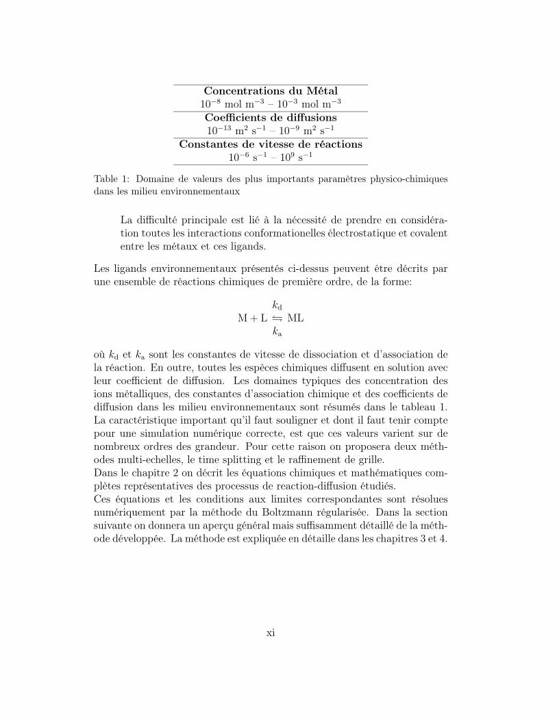
La méthode du raffinement de grille revient à utiliser plusieures grilles dansle domaine de calcul. Une tel choix est nécessaire lorsque des variations demasse importantes ont lieu à l’intérieur du domaine de calcul, par exem-ple dans le cas où certaines constantes de vitesse de réaction sont élevéeset les couches des réaction correspondantes très petites (parfois de l’ordrede manomètre). Il faut alors de fixer une taille de grille plus petite quel’épaisseur de la couche de réaction.Cette thèse propose une procédure de raffinement fondée sur la répartitiondu domaine de calcul en sous-grilles G1, . . . , Gs chacune avec une taille ∆xi etune discretisation temporel ∆ti. La figure 3 montre un cas 1D de raffinementavec s = 3. Les points A et D sont les points à la limite du domaine exploréet les points B et C sont les interfaces entre le sous-grilles G1-G2 et G2-G3.La procédure est basée sur la détermination des fonctions des distributionsinconnues aux points critiques B et C, en utilisant

• l’interpolation temporel et

• les lois de conservation de la masse et du flux.

xv

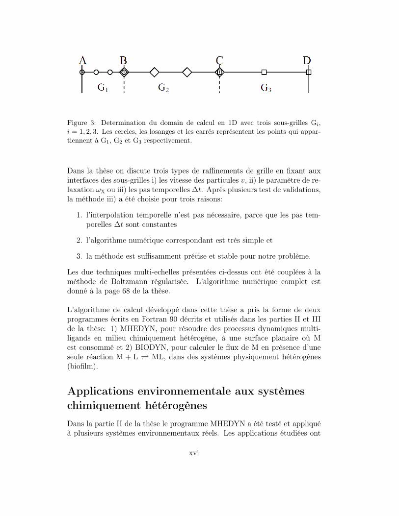
Figure 3: Determination du domain de calcul en 1D avec trois sous-grilles Gi,i = 1, 2, 3. Les cercles, les losanges et les carrés représentent les points qui appar-tiennent à G1, G2 et G3 respectivement.

Dans la thèse on discute trois types de raffinements de grille en fixant auxinterfaces des sous-grilles i) les vitesse des particules v, ii) le paramètre de re-laxation ωX ou iii) les pas temporelles ∆t. Après plusieurs test de validations,la méthode iii) a été choisie pour trois raisons:

1. l’interpolation temporelle n’est pas nécessaire, parce que les pas tem-porelles ∆t sont constantes

2. l’algorithme numérique correspondant est très simple et

3. la méthode est suffisamment précise et stable pour notre problème.

Les due techniques multi-echelles présentées ci-dessus ont été couplées à laméthode de Boltzmann régularisée. L’algorithme numérique complet estdonné à la page 68 de la thèse.

L’algorithme de calcul développé dans cette thèse a pris la forme de deuxprogrammes écrits en Fortran 90 décrits et utilisés dans les parties II et IIIde la thèse: 1) MHEDYN, pour résoudre des processus dynamiques multi-ligands en milieu chimiquement hétérogène, à une surface planaire où Mest consommé et 2) BIODYN, pour calculer le flux de M en présence d’uneseule réaction M + L ­ ML, dans des systèmes physiquement hétérogènes(biofilm).

Applications environnementale aux systèmes

chimiquement hétérogènes

Dans la partie II de la thèse le programme MHEDYN a été testé et appliquéà plusieurs systèmes environnementaux réels. Les applications étudiées ont

xvi

permis de vérifier les capacités de MHEDYN. MHEDYN est une programmefiable qui peut calculer les flux et les profils des concentrations de toutesles espèces chimiques présents en solution, même lorsqu’elles sont très nom-breuses avec des propriétés très différentes. Les principales caractéristiquesde MHEDYN sont les suivantes:

1. Calcul du flux de l’ion métallique étudié à une surface plane où il estconsommé en présence de réactions de complexations chimique avec desligands en nombre illimité et pouvant former des complexes successifs.

2. Capacité de travailler avec n’importe quelle valeur de concentration desligands, en excès ou non par rapport au métal considéré.

3. Calcul du flux du métal en fonction du temps et à l’état stationnaire.

4. Calcul du degré de labilité de chaque complexe.

5. Calcul des profils de concentration de chacune des espèces chimiquesprésentes en solution.

6. Capacité de travailler dans un domaine très large pour les valeurs desparamètres physico-chimiques. MHEDYN a été appliqué avec des ré-sultats très satisfaisants dans des solutions contenant un mélange deligands conduisant à des paramètres situés dans les domaines suivants:

• Coefficients de diffusions entre 2.4 × 10−13 et 7.1 × 10−10 m2s−1.

• Constantes de vitesse d’association entre 7.2 × 102 et 2.5 × 108

m3mol−1s−1.

• Constants d’équilibre entre 104.1 et 1016.1.

Application aux systèmes physiquement hétérogènes

(biofilm)

Dans la partie III de la thèse, le programme BIODYN a été testé et vérifiéavec des systèmes 3D simples et les résultats on montré un bon accord avecles solutions analytiques correspondantes. Le programme BIODYN a ensuiteété développé pour permettre d’effectuer des calcul en parallèl sur un clusterd’ordinateurs afin de pouvoir effectuer des calculs longs et demandant unegrande capacité de mémoire, comme c’est le cas pour les systèmes physique-ment hétérogènes naturels.L’algorithme complète est donné à la page 143. Il est appliqué à l’étude des

xvii

biofilms.Un biofilm est une couche de gel d’exoplymers organiques qui contient desmicroorganismes tels que des bactéries. Un biofilm est, en général, attachésur une surface inerte. Plusieurs processus influencent le fonctionnementd’un biofilm. En particulier:

• L’écoulement du fluid à la surface du biofilm.

• La convection, la diffusion et les réaction dans le biofilm.

• Le développement de micro-organismes et leur consommation/productiond’espèces chimiques dans le biofilm.

Dans la thèse on a choisit une modèle de biofilm simplifié, dans lequel on tientpas compte des processus de convection et de croissance des microorganismes.Ce choix est lié au domaine de temps (seconds-minutes) considéré pour lessimulations. Dans ces cas:

1. L’écoulement du fluid à la surface du biofilm est rapide et permit demaintenir une concentration constante à l’extérieur du gel du biofilm.

2. La croissance de micro-organismes est souvent beaucoup plus lente quele domaine de temps considéré.

La structure du biofilm est représentative de conditions naturelles et est don-née dans la figure de page 138.

Une caractéristique essentielle de BIODYN est de pouvoir simuler desflux à l’intérieur d’un biofilm, c’est à dire dans un milieu physiquementhétérogènes, possédant un grand nombre de micro-organismes sphériques àla surface desquels M est consommé. À la surface des microorganismes onapplique l’équation de Michaelis-Menten à l’état stationnaire.Les principales caractéristiques de BIODYN sont les suivantes:

1. Calcul du flux du métal M et des indices local de labilité du complexeML, à la surface de chaque microorganisme.

2. Calcul des profils de concentration de toutes les espèces chimiques dansles biofilms, à l’état stationnaire et en fonctionne du temps.

3. Calcul de la quantité de métal accumulé dans chaque micro-organismeen fonction du temps.

Dans le chapitre 8, différentes simulations préliminaires ont été effectuéessans changer la distribution (aléatoire) des micro-organismes. Les résultatsobtenu ont montré que:

xviii

1. L’échelle du temps nécessaire pour attendre un pseudo état station-naire dans un biofilm avec un cluster de microorganismes de 20µmd’épaisseur, est de l’ordre de 30 seconds - 1 minute.

2. L’indice de labilité local du complexe ML semble diminuer avec la pro-fondeur dans le cluster ou rester constant, selon les conditions de la-bilité. Il est en général plus faible qu’en solution homogène (indiquantque ML est moins biodisponible).

3. L’homogénéité de l’indice de labilité de ML dans le cluster sembledépendre de l’épaisseur de la couche de réaction par rapport au rayondes microorganismes.

Les résultats obtenu doivent être considérés comme préliminaires. Ils serontvérifiés soigneusement en étudiant les flux de M et l’indice local de labil-ité dans des conditions différentes. Néanmoins, le code BIODYN a montrésa capacité à effectuer des calculs de flux dans des systèmes physiquementhétérogènes compliqués, faisant intervenir des processus de réaction-diffusion.

xix

Chapter 1

Introduction

1.1 Motivation

This thesis is inspired from the wide complexity of the physical systems andconsequently by the necessity to simplify their complexity into fundamentalprocesses.It deals with a wide variety of physicochemical processes that take placein environmental systems, such as aquatic systems, porous media, sediment,soils and biofilm layer on inert substrate. In particular we focus the attentionon metal complexes in aquatic systems and biofilm structures (figure 1.1).In these systems, the values of the physicochemical parameters linked to themetal species, such as rate and equilibrium constants, or diffusion coefficients,may vary over orders of magnitudes depending on the nature of the chemicalligands and the physical structure of the medium.With the increase of computer power, both in terms of memory and rapidityof computation, the numerical modelling is becoming more and more anessential tool that can help to simulate the wide variety of real systems. Thepurpose of this thesis is to develop a new numerical computer algorithm basedon the Lattice Boltzmann approach which is applicable to environmentalchemical systems.The model developed in this thesis consider two processes coupled together:diffusion and chemical reaction. The general problem studied in this thesisis the set of reaction-diffusion equations for a metal M in a chemical solutionwith a collection of ligands and complexes. The specific purpose is to computethe flux of the metal M at a consuming surface, as bioanalogical sensors ormicroorganisms, and investigate the impact of complexation with ligands inenvironmental systems.

1

Figure 1.1: Schematic diagram of the physicochemical processes that take placenear a consuming surface, electrode or microorganism.

1.2 Environmental Processes

1.2.1 Chemically heterogeneous systems

The general framework of application of the work presented in this thesisdeals with the uptake, by a consuming surface, of metal ions complexed byenvironmental ligands, as described in figure 1.1. It shows schematically themost important physicochemical processes that take place in aquatic sys-tems, near a consuming surface, represented by a bioanalogical sensor or amicroorganism Many biophysicochemical processes in aquatic systems aredynamic [1, 2, 3]. For instance the biouptake of metals by microorganismsdepends on hydrodynamics, metal transfer through the plasma membraneand metal transport in solution by diffusion, as well as chemical kinetics ofcomplex formation/dissociation in solution [4, 5].Natural complexants include various types of compounds [6], often signifi-cantly more complicated than "simple ligands" such as OH−, CO2−

3 , aminoacids,oxalate, because both electrostatic and covalent interactions with the metalsneed to be considered. In general they can be classified as follows [6]:

1. Simple organic and inorganic ligands, which are often found in largeexcess compared to transition and b metals

2. Organic biopolymers, the most important of which are humic/fulviccompounds

2

3. Particles and aggregates in the size range 1-1000 nm, largely composedof inorganic solids such as clays, iron oxide etc.

Each type of complexant has its own specific properties which should beconsidered properly for correct computation of dynamic fluxes. These aspectsare discussed in detail in [7]. Key aspects to consider are briefly summarisedbelow:

• simple complexants are small sized, forming quickly diffusing com-pounds which are complexes, often labile or semi-labile, with weakto intermediate stability. Thus, when present, these complexes can beexpected to contribute to metal bioavailability. But this contributionis limited by their stability.

• Humics and fulvics are "small polyelectrolytes" (1-3 nm) with interme-diate diffusion coefficients, i.e. intermediate mobility. In addition theyinclude a large number of different site types, forming metal complexeswith widely varying stability and formation/dissociation kinetics. Thusthe corresponding contribution to the flux is expected to depend largelyon this chemical heterogeneity through the metal/ligand ratio under thegiven conditions.

• Particulate complexants are often aggregates of various particles andpolymers. Thus they may be also chemically heterogeneous, eventhough relatively chemically homogeneous particles may also be found.The important sites of particles (e.g. -FeOOH sites on iron oxide)form complexes with intermediate to strong stability and intermediateto slow chemical kinetics. The key property of these particles is thattheir size distribution is often very wide, i.e. their diffusion coefficientmay vary from intermediate to very low values. So it is expected thattheir contribution to bioavailability will be largely dependent on thesize class.

The computation of metal flux, at consuming interfaces, in complicated envi-ronmental systems including many ligands, is a difficult task due to the manycoupled dynamic physical and chemical processes. Theoretical concepts havebeen developed long time ago [8, 9] to compute a metal flux regulated byreaction-diffusion processes at consuming voltammetric electrodes, in solu-tion containing a single ligand. Such theories and concepts have been appliedmore recently to bioanalogical sensors and biouptake [10, 11]. Theories havealso been extended recently to the case of solutions containing many ligands[12, 13].However, most papers refer to 1/1 ML complexes with simple ligands, with

3

exceptions of a few ones [14] dealing with successive complexes. In addition,the ligand, in most cases, is considered as being in excess compared to thetotal metal concentration.As far as computation codes are concerned, the situation of metal flux dy-namic computation is at odds with the case of thermodynamic distribution ofmetal complexes for which a wealth of codes have been developed [15, 16]. Toour knowledge only one code has been published [17] for metal flux compu-tation in presence of large mixtures of ligands, which considers a wide rangeof chemical kinetics and diffusion coefficients, as it is usually the case in nat-ural waters. However, it is applicable only in excess of ligands compared tometal. Moreover, it has not yet been applied to aquatic systems includingenvironmental ligands under realistic conditions of pH and concentrations.

1.2.2 Physicochemical complex geometry: Biofilm

Sediments, soils, thin-films and biofilms are all complex systems in whichseveral physical and/or chemical and/or biological processes can take placesimultaneously. Several simulation models exist in the literature, for instancein sediments and soils [18] and biofilms [19, 20].In chapter 8 of this thesis, we focus on the numerical simulation of biofilms.They are characterised by:

1. Complex and extremely variable geometry. Their size may be close tothat of a single cell (µm) or extend to several meters.

2. Different nature. They can be formed by bacteria, mussels, worms orsimple prokaryotic cells, with diameters of few micrometres.

3. Complex processes coupled together. Inside a biofilm one can observemany processes taking place simultaneously like fluid flowing throughchannels, transport of oxygen and substrates into the biofilm, redoxreactions and reaction-diffusion of metal complexes.

4. Dynamical behaviour. Biofilms are not static entities, but they slowlychange in size and structure under growing or detachment processes.

In order to evaluate such systems, mathematical models can be very useful,but their complexity is very high, like those proposed in [21] so simplifiedmodels have also been developed [22]. A complete approach for two- andthree-dimensional biofilm growth and structure formation has been devel-oped in [20] by taking into account hydrodynamics, convection-diffusion masstransfer of soluble components, biomass increase, decay and detachment.However, to our knowledge, no numerical simulation has been performed to

4

study trace metal fluxes at the bacteria surface in a biofilm cluster and theirrelationship with complexing agents.In this thesis we have developed a simplified 3D biofilm model in which dif-fusion of M and reaction with a ligand L (in excess) is present and where theuptake of M, by each microorganism in the biofilm, can be studied.

1.3 The method proposed

In this thesis, we will propose a numerical method based on the LatticeBoltzmann approach that can be applied to compute metal fluxes in presenceof such ligands and their mixture, and to estimate the relative impact ofeach type of complex on the overall metal flux at a consuming surface (e.g.organism or bioanalogical dynamic sensor).The processes illustrated in figure 1.1 belong to the wide class of Multiscaleprocesses, because their physicochemical parameters vary in a wide rangeof values. In order to deal with these types of processes, we will develop aprocedure that couples the Lattice Boltzmann approach with two standardtechniques:

• The time splitting method, to discriminate fast from slow processes [23]

• The grid refinement method, to localise and resolve large variations ofgradient concentrations [24]

The numerical algorithms, based on the Lattice Boltzmann Methods, havebeen applied to many complex systems [25] and have shown good accuracyfor the reproduction of fluid flow systems [26, 27, 28]. Only a few applicationshave been performed for reaction-diffusion systems [29, 30] and no compu-tational codes are at the moment available for the community of chemists.We believe that this work can be of support to the community of chemistsinvolved in this kind of problems. In particular, this thesis proposes twocodes, stemming from the same algorithm:

1. MHEDYN - To compute metal fluxes at planar consuming surfaces inmultiligand, chemically heterogeneous environmental systems.

2. BIODYN - To compute metal fluxes in 3D biofilm models

MHEDYN has been successfully tested with an other program code (FLUXY,[17])based on approximate formulas and valid only at steady-state and in excessof ligands. At the moment, MHEDYN is not user-friendly yet, but there isa project to render MHEDYN accessible to the community of environmental

5

chemists.BIODYN can perform flux computations by running in parallel on severalprocessors. At the moment, only preliminary tests have been successfullyperformed by comparing its results with simple 3D benchmarks. Other testshave to be done in the future to check its real accuracy and performance.The codes are written in Fortran 90 and they are both available on the webat the following address: http://cui.unige.ch/∼alemani.

1.4 Organisation of the thesis

The thesis is organised in three parts.Part I describes the physicochemical problem and explains the numericalmodel used to simulate reaction-diffusion processes.Part II shows qualitatively and quantitatively validations of the numericalcode and report detailed computations in multiligand and chemically hetero-geneous systems.Part III validates the code for 3D systems and shows a 3D application to asimple biofilm model.In part I:Chapter 2 describes the physical problem focusing on its wide range of spaceand time scales. In this sense, the problem is classified as a typical multiscaleproblem. At the end of the chapter the mathematical formulation is givenwith the initial and boundary conditions.Chapter 3 describes the Lattice Boltzmann Method used to solve reaction-diffusion processes. A new method is described based on the regularisedapproach.Chapter 4 describes and validates two techniques that are coupled with theLattice Boltzmann Method to solve a typical multiscale system: the timesplitting and the grid refinement methods.In part II:Chapter 5 gives some chemical examples to validate the numerical algorithmdeveloped in the previous chapter.Chapter 6 applies the numerical code to solve environmental chemical sys-tems: i) simple ligands, like CO2−

3 and OH−, ii) Fulvic acids and iii) sus-pended particles /aggregates, iv) mixtures of ligands i) to iii). In this chapterwe computed the metal flux and the lability degree for many examples of realchemical conditions.In part III:Chapter 7 gives some 3D examples in order to qualitatively and quantita-tively validate the numerical code for 3D applications.

6

Chapter 8 applies the code to a 3D biofilm model.

1.5 Publications

The work performed during this PhD thesis has produced the following pub-lications:

1. P. Albuquerque, D. Alemani, B. Chopard, and P. Leone. Coupling aLattice Boltzmann and a Finite Difference Scheme. In M. Bubak, G.D.van Albada, P.M.A. Sloot, and J.J. Dongarra, editors, ComputationalScience - ICCS 2004: 4th International Conference, Kraków, Poland,June 6-9, 2004, Proceedings, Part IV, volume 3039, page 540. SpringerBerlin / Heidelberg, 2004.

2. P. Albuquerque, D. Alemani, B. Chopard, and P. Leone. A hybridLattice Boltzmann Fnite Difference scheme for the Diffusion Equation.To appear in International Journal for Multiscale Computational En-gineering, Special Issue, 2004.

3. D. Alemani, B. Chopard, J. Galceran, and J. Buffle. LBGK methodcoupled to time splitting technique for solving reaction-diffusion pro-cesses in complex systems. Phys. Chem. Chem. Phys., 7:3331–3341,2005.

4. D. Alemani, B. Chopard, J. Galceran, and J. Buffle. Time splittingand grid refinement methods in the Lattice Boltzmann framework forsolving a reaction-diffusion process. In V.N. Alexandrov, G.D. vanAlbada, P.M.A. Slot, and J.J. Dongarra, editors, Proceedings of ICCS2006, Reading, LCNS 3992, pages 70–77. Springer, 2006.

5. D. Alemani, B. Chopard, J. Galceran, and J. Buffle. Two grid re-finement methods in the Lattice Boltzmann framework for reaction-diffusion processes in complex systems. Phys. Chem. Chem. Phys.,8:4119–4130, 2006.

6. D. Alemani, B. Chopard, J. Galceran, and J. Buffle. Study of three gridrefinement methods in the Lattice Boltzmann framework for reaction-diffusion processes in complex systems. Submitted to InternationalJournal for Multiscale Computational Engineering, Special Issue, 2007.

7. D. Alemani, B. Chopard, J. Galceran, and J. Buffle. Metal Flux compu-tation in environmental ligand mixtures: simple, fulvics and particulatecomplexants. In preparation., 2007.

7

8. D. Alemani, B. Chopard, J. Galceran, and J. Buffle. Metal fluxes inbiofilms. In preparation., 2007.

8

Part I

The model and Validation

9

Chapter 2

The Physical Problem

2.1 Overview

In this chapter, the physical problem to be investigated is defined.In section 2.2, we study the complex reaction-diffusion problem of a metal Mwith a number of ligands by introducing a basic prototype problem, taken asmodel, for which a mathematical formulation will be given. Space and timescales of the prototype model are defined and discussed.In section 2.3, a summary of the typical ranges of the physicochemical pa-rameters is given. We will see that the prototype model is considered atypical multiscale problem, due to the large variations of its physicochemicalparameters.Finally section 2.4 gives the mathematical formulation of the problem withthe governing equations and the initial and boundary conditions.

2.2 The Problem

As we have seen in the previous chapter, reaction-diffusion processes arecommon in environmental chemistry and biological systems. They can behighly non-linear, involve many species and often take place in complicatedgeometries. As a consequence, several time and spatial scales characterisethe processes and accurate numerical solutions are difficult to obtain.The general environmental reaction-diffusion problem involves the solutionof a set of complexation reactions for a metal M in a heterogeneous systemwith several ligands of different nature. For instance a metal M can reactsimultaneously with a first ligand 1L and a second ligand 2L:

M + 1L ­ M1L

M + 2L ­ M2L(2.1)

11

Element Open sea waters (mol m−3) Fresh waters (mol m−3)Mn 10−7 – 10−5 10−6 – 10−2

Fe 10−7 – 10−5 10−4 – 10−2

Ni 10−6 – 10−3 10−6 – 10−3

Cu 10−6 – 10−3 10−6 – 10−3

Zn 10−8 – 10−3 10−6 – 10−3

Cd 10−9 – 10−4 10−7 – 10−5

Pb 10−8 – 10−4 10−7 – 10−3

Table 2.1: Ranges of the typical concentration values of the more important metalion M (page 2, from [1])

The ligands 1L and 2L may have completely different chemical properties,different diffusion coefficients and may or may not be in large excess withrespect to M. The reaction of M with different ligands is called parallel com-plexation, because the metal M in solution can bind with two or more ligandsat the same time.Moreover, each complex can react with the same ligand to generate a newcomplex and so on, via a set of successive reactions. For instance, consideringthe above mentioned reactions, M1L may bind with 1L and M2L may bindwith 2L:

M1L + 1L ® M1L2

M2L + 2L ® M2L2

(2.2)

The subscript of L refers to the stoichiometry of L in the complex. The typeof reactions (2.2) is called successive or sequential complexation reactions.Parallel and successive complexation reactions are very typical in environ-mental chemical solutions. Such reactions are a simplification of the realenvironmental processes that occur in nature, nevertheless until now, no dy-namic numerical simulation that takes into account both types of reactions(2.1) and (2.2) at the same time has been developed at our present knowledge.

2.2.1 The prototype problem

In this thesis we focus the attention on aquatic systems.In open sea waters and fresh waters the concentration of inorganic elementsvaries on a very wide range over orders of magnitude [1]. Table 2.1 shows thatthe concentrations of important trace metal ions range from 10−9 mol m−3

up to 10−2 mol m−3. In environmental systems, trace metals are found indifferent forms, including free hydrated ions, and complexes with well-known

12

inorganic ligands, with poorly defined natural ligands or as adsorbed specieson the surfaces of particles and colloids [6]. Their chemical reactions in theexternal medium greatly influence their biological effects [5].The basic process of adding a ligand to a free metal or a complex is the samefor parallel and successive reactions and can be reduced to the simple 1:1reaction:

M + L ­ ML (2.3)

It is important, therefore, to understand the basics of this simple process inorder to fully understand the behaviour of more complicated systems.Thus, as a first step, the discussion below is focused on the prototype prob-lem under planar diffusion. Most properties and considerations made for aplanar geometry are valid also for spherical geometry. Moreover, planar dif-fusion is also adequate to describe spherical diffusion, provided the sphereradius is large enough and the time domain of interest is small enough. Forinstance, for a sphere of radius r0, the planar diffusion is accurate within a%

if δr0

≤ a100

1.The prototype problem is shown in figure 2.1 which depicts concentration

Figure 2.1: Schematic representation of the physicochemical problem. The metalion M can form a complex ML with a ligand L, having stability constant K, anassociation rate constant ka and a dissociation rate constant kd. Each of the threespecies diffuse in solution. M can also be consumed at the interface through variousreactions (see text). The diffusion layer, δ, is the region in the vicinity of theconsuming surface where the concentration is significantly different from the bulkvalue. The reaction layer µ is such that any M dissociated from ML is supposedto be consumed at the interface more quickly than recombined to L.

1δ is the diffusion layer of the metal in solution. Its definition is given in section 2.2.2

13

profiles of M and ML at the surface of a consuming sensor or organism. Oneof the most interesting and important physicochemical and biological tasks isto understand the role played by chemical complexations and physical trans-port of M and ML in the surrounding environment of the sensor or organismwith regards to their uptake. As shown in figure 2.1, the metal ion M insolution can form a complex ML with a ligand L via reaction (2.3), withequilibrium constant K and association and dissociation rate constants ka

and kd. M, ML and L diffuse in solution with diffusion coefficients DM, DML

and DL. The plane x = 0 contains a surface which consumes M but notML or L. If the consuming surface is a Hg voltammetric electrode, M canbe reduced into the metal species M0 via the redox reaction M+ne− ® M0,when a sufficiently negative potential E is applied. Then M0 diffuses in theamalgam (extension to diffusion in the same solution is straightforward) withdiffusion coefficient DM0 . On the other hand, if the consuming surface is amicroorganism, the metal M first binds with a complexing site at the surfaceof the membrane and is then internalised inside the microorganism. Thisprocess is the so-called Michaelis-Menten mechanism [5].The mathematical formulation of the planar reaction-diffusion prototypeproblem in presence of an Hg voltammetric electrode and a consuming or-ganism is given below.

The governing equations in planar geometry

The equilibrium constant of the reaction (2.3), K = kakd

expresses the relationbetween M, L and ML in the bulk solution

K =[ML]∗

[M]∗[L]∗

where [X]∗ are the bulk concentrations of the species X=M, L and ML re-spectively.Relevant environmental cases are those where [ML]∗ ≥ [M]∗, i.e. K[L]∗ ≥ 1,and where [L]∗tot ≥ [M]∗tot.In order to compact the notation, we introduce the functions [X]=[X](x, t),with X=M, L, ML and M0, which represent the values of the concentrationsof the species involved in the processes.The planar semi-infinite diffusion-reaction problem for the species M, L andML, is described by the following system of partial differential equations inthe x -axis, ∀t > 0:

∂[M]

∂t= DM

∂2[M]

∂x2+ RM (2.4)

14

∂[ML]

∂t= DML

∂2[ML]

∂x2+ RML (2.5)

∂[L]

∂t= DL

∂2[L]

∂x2+ RL (2.6)

∂[M]0

∂t= DM0

∂2[M]0

∂x2(2.7)

where the RX’s with X=M, L and ML are the rates of formation of M, L andML respectively:

RM = kd[ML] − ka[M][L] (2.8)

RL = RM (2.9)

RML = −RM (2.10)

Equations (2.4) - (2.6) are defined ∀x ∈ (0, +∞), while equation (2.7) isdefined ∀x ∈ (−∞, 0).

2.2.2 Space scales: Diffusion and reaction layer thick-nesses

It is important to introduce here two crucial space scale parameters, con-nected with the physicochemical properties, which describe the spatial be-haviour of the system: the diffusion layer thickness δM and the reaction layerthickness µML.As schematically depicted in figure 2.1, the diffusion layer can be under-stood for each species as the region in the vicinity of an electrode where theconcentration is significantly different from its bulk value. The value of thediffusion layer thickness depends on the consumption of M at the surface, onits diffusion coefficient on time and on hydrodynamic conditions. In manycases, in unstirred solutions, δM, can be expressed as [31]:

δM =√

πDMt (2.11)

where t is the total time in which diffusion occurs.The reaction layer is associated with the formation rate of a complex ML.Its thickness, µML, corresponds to the distance from the consuming surfacebeyond which the deviation from the chemical equilibrium is taken to benegligibly small. Outside this layer, when M dissociates from ML, it can beonly recombined to L after some short time. Inside this layer, the dissociatedM is more often consumed at the interface than recombined to L. The value

15

of µML depends on the ratio of the diffusion rate of M over its recombinationrate with L [31]:

µML =

√

DM

ka[L]∗(2.12)

where [L]∗ is the bulk concentration of L.For fast reactions (ka large), this distance is a very thin layer. For interme-diate ka values, the rate of the chemical reaction plays a key role on the fluxof the metal ion M towards the interface at x = 0.The thicknesses of δM and µML influence the numerical simulation of thereaction-diffusion process by playing a crucial role in the choice of the valueof the grid size. In general, it has to be less than the minimum value takenby either µ or δ in order to be able to accurately resolve the concentrationgradients of all the species, close to the consuming surface 2. (Typical rangesof values will be given in table 2.3.)

2.2.3 Diffusion and reaction time scales

Other two important parameters are essential to describe the behaviour ofthe system: the reactive and the diffusive time scales.The time scales of reaction can be defined by the recombination rate of Mwith L

tR =1

ka[L]∗(2.13)

On the other hand, the time scale of diffusion is described by combining theexpression of the diffusion layer (2.11) with the diffusion coefficient, [6]

tD =δ2M

DM

(2.14)

Relevant cases are those for which the time scale of reaction is smaller orcomparable to the time scale of diffusion. Diffusion coefficients of metalsand complexes range in between 10−12 m2 s−1 and 10−9 m2 s−1, so that thecorresponding time scale is tD = 10−5 − 100s.Kinetic rate constants ka can range from very low to very high values, usu-ally in between 10−6 and 109m3mol−1s−1, so that the time scale of complexformation, equation (2.13), ranges in between 10−8s and days. If tR À tDthen the complex is inert and only diffusive processes are important, whilefor tR < tD diffusion and reaction both influence the flux.

2In chapter 4 this condition is explained with a model example.

16

In order to understand the influence of the complexation reaction on the flux,the flux computed in the tested conditions will be compared to:

1. The equally mobile and labile flux, Jmax:

Jmax =DM[M]∗tot

δM

(2.15)

2. The "inert" flux, Jin:

Jin =DM[M]∗

δM

(2.16)

3. The "labile" flux, Jlab:

Jlab =DM[M]∗tot

δM

(2.17)

The mobile-labile flux, Jmax, is the case corresponding to the labile flux andhypothetical equal diffusion coefficients, i.e. DML = DM. The inert flux, Jin,is the flux which would be obtained if the complex was inert, i.e. does notdissociate at all. It is equal to the diffusive flux of M without L, at the bulkconcentration [M]∗. The labile flux, Jlab, is the flux which would be obtainedif metal and complexes were fully labile. It is equal to its diffusive flux, withan average diffusion coefficient defined as [13]:

DM =

∑

i DMLi[ML]i∗

[M]∗tot(2.18)

for a fixed ligand L. The computation of the fluxes introduced above, enablesto determine the lability of a complex ML, i.e. how much it affects the to-tal flux of M and to establish its bioavailability in the surrounding solution[1, 32, 6, 5].We investigate several examples of simple and complex processes in a multi-ligand context in chapter 6.

2.3 A typical Multi-scale problem

To complete the general description of the prototype problem, table 2.2 givesa summary of the typical range of metal concentrations, diffusion coefficientsand kinetic rate constants for an environmental problem. As we can see,the trace metal concentrations vary on a wide range of values (as we havealready seen in table 2.1), the diffusion coefficients are low and they vary on

17

Metal Concentrations10−8 mol m−3 – 10−3 mol m−3

Diffusion Coefficients10−12 m2 s−1 – 10−9 m2 s−1

Kinetic Rate Constants10−6 s−1 – 109 s−1

Table 2.2: Range values of the main physicochemical parameters for the typicalreaction diffusion process (2.3)

Space TimeReaction µ (ka[L]∗)−1

10−9m ÷ 10−3 m 10−8s ÷ 100 sDiffusion δ δ2/D

10−7m ÷ 10−3 m 10−4 ÷ 100 s

Table 2.3: Typical ranges of diffusion and reaction layers and diffusion and reactiontimes in environmental systems.

three orders of magnitude and the complexation kinetic rate constants varysignificantly in a range of fifteen orders of magnitude.The four parameters, δM, µML, tR and tD (equations (2.11), (2.12), (2.13) and(2.14)) are essential to describe the space-time scales of the processes involvedin the system. Their values influence the physicochemical properties of anenvironmental systems and they are useful to determine the rate-limitingprocesses of the system.Let us consider a typical set of values wherein the bulk concentration of L, [L]∗

is in excess compared with the bulk concentration of M, [M]∗: [M]∗ = 10−3molm−3, [L]∗ = 1mol m−3, DM = 10−9m2s−1 and ka[L]∗ = 108s−1. If consump-tion of M at the planar surface is very fast, a diffusion gradient is establishedclose to the electrode surface. After one second, the four key parameterstake the following values: µ ∼ 3nm, δ ∼ 60µm, (ka[L]∗)−1 = 0.01µs andδ2M/DM ∼ 3s. Thus, clearly, the reaction and the diffusion processes take

place at very different scales. For this reason the prototype problem (2.3) isconsidered as an example of typical multiscale process.Table 2.3 gives the typical ranges of space and time scales which are metin environmental systems. Diffusive space scales range usually from submi-crometers to mm, depending on the geometry and diffusion coefficient of thespecies. Reactive space scales take very different values depending on thecomplexation reaction rates. They can take values as small as 1-10nm, for

18

fully labile complexes. Such very small values are the most important limit-ing factor in terms of computer memory. This is because the grid sizes haveto be chosen sufficiently small to follow the large concentration variations ofthe species involved in that space scales.In order to localise and compute accurate concentration profiles in a thinlayer of solution close to the interface, the grid should be refined within thespecific region. The corresponding numerical methods are known in litera-ture as grid refinement methods. In chapter 4 we describe different types ofgrid refinement methods in the framework of the lattice Boltzmann scheme.Table 2.3 also shows typical time scales of reaction and diffusion under en-vironmental conditions. Typical reaction time scales can vary between 10−8

and 100 s−1. The smallest values, corresponding to fully labile complexes,are the limiting factors in terms of computational time, since the computa-tional time step should be short enough to ensure a sufficient accuracy. Forthis reason, a suitable numerical method, enabling to discriminate slow andfast processes, is necessary. In chapter 4 we explain how to apply the timesplitting method in the Lattice Boltzmann context to separate fast from slowprocesses and solve them with appropriate numerical procedures.Multiscale problems are often met in real systems and they always representa big challenge for the numerical simulation community. For that reason, asimplification is needed which on the one hand reduces the computationalcost and the computer memory usage and, on the other hand, maintains asufficient accuracy of the solution.In order to achieve such a task, this thesis proposes to introduce the timesplitting method and three different grid refinement techniques in the Lat-tice Boltzmann framework for solving reaction-diffusion systems, not onlyfor environmental or electrochemical applications but in general for a largercommunity of scientists that are interested in simulating and understandingmultiscale phenomena.

2.4 The mathematical formulation of the prob-

lem for Multiligand applications

2.4.1 Reaction-Diffusion equations

Let us suppose that the system includes nl ligands and jn successive com-plexation reactions for each type of ligand, with j = 1, . , nl. We will consider

19

a set of parallel and successive chemical reactions of the following kind:

M + jL

jkd,1

®jka,1

MjL (2.19)

MjLi−1 + jL

jkd,i

®jka,i

MjLi i = 2, · · · ,j n (2.20)

Chemical reactions (2.19) and (2.20) take place within the solution domain.Index i represents the stoichiometric number of jL in the complex and thesuperscript j is limited to the nature of the ligand. The chemical rate asso-ciated to each reaction is given by:

jri = −jka,i[MjLi−1][

jLi] + jkd,i[MjLi] (2.21)

where jka,i and jkd,i are the association and dissociation rate constants re-spectively. The association and dissociation rate constants define the equi-librium constant for each reaction, jKi. It is defined as:

jKi =jka,i

jkd,i

=[MjLi]

∗

[MjLi−1]∗[jLi]

∗ i = 2, . . . , jn (2.22)

The first equilibrium constant jK1 is:

jK1 =jka,1

jkd,1

=[MjL]∗

[M]∗[jL]∗(2.23)

All the species diffuse within the solution domain following the usual set ofreaction-diffusion equations:

∂[M]

∂t= DM∇2[M] +

nl∑

j=1

jr1 (2.24)

∂[jL]

∂t= DjL∇2[jL] +

jn∑

i=1

jri (2.25)

∂[MjLi]

∂t= DMjLi

∇2[MjLi] − jri + jri+1 i = 1, . . . , jn − 1 (2.26)

∂[MjL]s∂t

= DMjLs∇2[MjL]s − jrs s = jn (2.27)

20

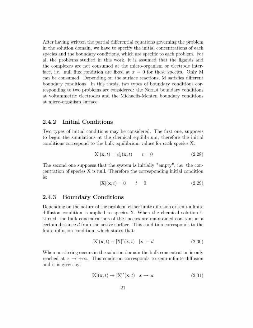
After having written the partial differential equations governing the problemin the solution domain, we have to specify the initial concentrations of eachspecies and the boundary conditions, which are specific to each problem. Forall the problems studied in this work, it is assumed that the ligands andthe complexes are not consumed at the micro-organism or electrode inter-face, i.e. null flux condition are fixed at x = 0 for these species. Only Mcan be consumed. Depending on the surface reactions, M satisfies differentboundary conditions. In this thesis, two types of boundary conditions cor-responding to two problems are considered: the Nernst boundary conditionsat voltammetric electrodes and the Michaelis-Menten boundary conditionsat micro-organism surface.

2.4.2 Initial Conditions

Two types of initial conditions may be considered. The first one, supposesto begin the simulations at the chemical equilibrium, therefore the initialconditions correspond to the bulk equilibrium values for each species X:

[X](x, t) = c∗X(x, t) t = 0 (2.28)

The second one supposes that the system is initially "empty", i.e. the con-centration of species X is null. Therefore the corresponding initial conditionis:

[X](x, t) = 0 t = 0 (2.29)

2.4.3 Boundary Conditions

Depending on the nature of the problem, either finite diffusion or semi-infinitediffusion condition is applied to species X. When the chemical solution isstirred, the bulk concentrations of the species are maintained constant at acertain distance d from the active surface. This condition corresponds to thefinite diffusion condition, which states that:

[X](x, t) = [X]∗(x, t) |x| = d (2.30)

When no stirring occurs in the solution domain the bulk concentration is onlyreached at x → +∞. This condition corresponds to semi-infinite diffusionand it is given by:

[X](x, t) → [X]∗(x, t) x → ∞ (2.31)

21

At the consuming surface S, there is no flux of MjLi and jLi crossing theinterface. Therefore:

(∂[MjLi]

∂n

)

x∈S= 0 (2.32)

(∂[jLi]

∂n

)

x∈S= 0 (2.33)

where n is the normal vector of the surface.

Two types of boundary conditions for M are considered at the consumingsurface. They are described below.

Interfacial boundary condition for M: Nernst equation

For the voltammetric sensor, the Nernst boundary condition is considered.The metal M can be reduced at the electrode interface into its neutral formM0, via the following redox process:

M0 n−

e

­ M (2.34)

where ne is the number of electrons involved in the redox reaction. If aconstant potential is applied at the electrode and the redox process can beconsidered reversible, then the Nernst condition applies:

[M](t) = [M0](t)e(E−E0)nef at x = 0 (2.35)

where E0 is the standard redox potential for the couple M/M0 and f isthe Faraday reduced constant (f = F

RT= 38.92V −1). In the above equation

another species has been introduced M0. Hence, another boundary expressioninvolving M0 and/or M is necessary in order to solve the set of reaction-diffusion equations. This additional boundary condition comes from the fluxconservation at the electrode surface. It is given by:

DM∂[M]

∂n= D0

M

∂[M0]

∂nx ∈ S (2.36)

The reduced form M0 is present only inside the electrode and its evolutionis followed by solving an appropriate diffusion equation:

∂[M0]

∂t= DM0∇2[M0] (2.37)

To solve equation (2.37), an additional boundary condition for M0 is neededat either x = −r0 (micro-electrode) or x → −∞ (macroscopic electrode). Inthe following, most problems consider the potential ∆E = E−E0 ¿ −0.3V .Under this assumption the electrode surface acts as a perfect sink for M andequation (2.37) involving M0 can be disregarded.

22

Interfacial boundary condition for M: Michaelis-Menten equation

If the consuming surface S is a micro-organism, the mechanism of site ad-sorption and internalisation is described by the Michaelis-Menten equation.This equation gives the internalisation flux of M as a function of its volumeconcentration near the surface.The general form of the Michaelis-Menten equation for a metal M is given in[33]:

Rtotd

dt

Ka[M ]

1 + Ka[M ]= DM∇n[M ] − kintRtotKa

[M ]

1 + Ka[M ](2.38)

where kint is the internalisation rate constant (s−1), Ka is the adsorptionconstant of M on the sites at the membrane surface (m3mol−1), Rtot is thesurface concentration of the free sites for the binding/transport of M (molm−2). For the application on biofilms we will show in chapter 8 that theassumption of steady-state for the Michaelis-Menten equation is reasonable.Therefore, its expression is given by:

Jint =1

A

dN

dt=

kintKaRtot[M]

1 + Ka[M]x ∈ S (2.39)

where Jint = JM is the internalisation flux, A is the surface area (m2), N isthe number of moles of M passing through the interface S, t is the time (s),and [M] is the volume concentration of M (mol m−3).Equation (2.39) is a mixed type boundary condition. Indeed, equation (2.39)contains both the flux of M at the surface, Jint and the concentration of M,[M]. Therefore, the version of equation (2.39) in terms of mixed boundarycondition takes the following form:

DM∇n[M] =KaRtotkint[M]

1 + Ka[M](2.40)

The above equation is a (non linear) combination of [M] and its normalderivative at the surface S of the micro-organism, ∇n[M].

2.5 Summary

In this chapter the general physical problem was introduced by focusing theattention on the prototype model, equation (2.3).The space and time scales has been described in relation with the diffusive

23

and reactive processes.The typical values of the physicochemical parameters were given, in partic-ular the range of values of concentrations, diffusion coefficients and reactionrate constants has been listed.Due to the large variations of the physicochemical parameters, the prototypemodel can be understood as a typical multiscale problem, requiring specificnumerical techniques to be solved.In order to numerically solve this kind of multiscale process, accurate meth-ods should be envisaged. Two typical and well known techniques that answerto our requests are the time splitting methods and the grid refinement tech-niques. A description of them is given in chapter 4.In the following chapter, the numerical scheme suggested to solve the gov-erning equation stated in section 2.4, is described.

24

Chapter 3

The Lattice Boltzmann Methodfor Reaction-Diffusion Processes

3.1 Overview

This chapter is organised as follows. Section 3.2 is an introduction to the stan-dard Lattice Boltzmann (LB) model. In section 3.3 the Lattice Bhatnagar-Gross-Krook model (LBGK) is described for solving reaction-diffusion pro-cesses. In particular, the attention is focused on the regularised LBGK model.In section 3.4 the standard LBGK model is compared with the regularisedLBGK model by studying the convergence conditions for the prototype prob-lem. Finally, in section 3.5 the numerical initial and boundary conditions arediscussed for the LBGK reactive-diffusive model.

3.2 The Lattice Boltzmann Approach

A lattice Boltzmann (LB) model [25, 26, 34, 29] describes a physical systemin terms of a mesoscopic dynamics. Intuitively we may think of fictitious par-ticles moving synchronously on a regular lattice, according to discrete timesteps. An interaction is defined between the particles that meet simultane-ously at the same lattice site. Particles obey collision rules which reproduce,in the macroscopic limit, an equation of physics. After the interaction, whichis assumed to be instantaneous, particles jump to one of the neighbouringsites, according to their new direction of motion. This propagation-collisionprocess is then repeated as many time as desired.In the last decade, the LB approach has met significant success in simulatinga wide range of phenomena. For instance, many applications can be foundin [35, 36, 27, 37, 38, 28, 25, 39]. The LB method has been successfully used

25

to simulate complex flow problems [26, 28, 40], reaction-diffusion systems[30, 36, 41, 42, 43], wave propagation processes [25] and reactive-diffusive-advective processes in porous media [44, 45, 46, 47].The major advantage of these methods over traditional numerical techniques,such as finite difference or multigrid techniques [48, 49, 50], finite elementmethods [51, 52, 53] or boundary element methods [54], is that they pro-vide insight into the underlying microscopic dynamics of the physical systeminvestigated, whereas most of the methods listed above, focus only on thesolution of the macroscopic equations. For instance, we will show a ’natural’way to compute the flux by using microscopic functions, which avoids thecalculation of the gradient of macroscopic functions. Note however that, LBhas not been extensively used in the reaction-diffusion field yet, because ithas no major advantage for systems with only one or two reactions like theprototype reaction, expression (2.3), and for simple geometry, which are thelarge majority of cases reported in the literature up to now.A LB model can be interpreted as a discretization of the Boltzmann trans-port equation on a regular lattice of spacing ∆x along each lattice directionand with discrete time step ∆t [55]. The possible velocities for the pseudo-particles are the vectors vi. They are chosen so as to match the latticeconstraints: if x is a lattice site, x+vi∆t is also a lattice point. The dynam-ics involves z +1 possible velocities, where z is the coordination number andv0 = 0 describes the population of rest particles. The lattice is identified byits spatial dimension d and its coordination number z indicating how manyneighbours each lattice point has. Traditionally, the lattice is then referredto as a DdQz lattice (D stands for Dimension and Q for Quantities).For isotropy reasons the lattice topology must at least satisfy the conditions[25, 29]:

∑

i

viα = 0 and∑

i

viαviβ = v2C2δαβ (3.1)

where C2 is a numerical coefficient which depends on the lattice topology.The Greek indices label the spatial dimension and v = ∆x/∆t. The firstcondition follows from the fact that if vi is a possible velocity, then so is −vi.In the LB approach a physical system is described through density distribu-tion functions fi(x, t). For hydrodynamics and reaction-diffusion processes,fi(x, t) represents the distribution of particles entering a site x at time t andmoving in direction vi. Therefore, in a LB approach, the description is finerthan e.g. in a finite difference scheme, as information on the particle micro-scopic velocity is included. As it can be shown, an important consequence ofthis fact is that the fi’s also contain information on the spatial derivatives ofthe macroscopic quantities. Physical quantities can be defined from moments

26

of these distributions. For instance, the local density is obtained by

ρ =z

∑

i=0

fi (3.2)

A LB model is determined by specifying:

• A lattice

• A general kinetic equation

fi(x + vi∆t, t + ∆t) − fi(x, t) = Ωi

where Ωi is the collision term that must preserve the conservation lawsof the system. For instance, in a diffusion process, particle number isconserved and, in a fluid, momentum is also conserved. In its simplestform (BGK model), the dynamics can be written as a relaxation to agiven local equilibrium

fi(x + vi∆t, t + ∆t) − fi(x, t) = ω(f eqi (x, t) − fi(x, t)) (3.3)

where ω is a relaxation parameter, which is a free parameter of themodel.

• An equilibrium distribution f eqi , that contains all the information con-

cerning the physical process investigated. It depends only on the lo-cal values of the macroscopic quantities and it changes according towhether we consider hydrodynamics, reaction-diffusion or wave propa-gation. For reaction-diffusion processes it takes the form [29]

f eqi (x, t) =

[X](x, t)

2d(3.4)

where [X](x, t) is the volume concentration of X.

3.3 The Lattice Boltzmann Reaction-Diffusion

Model

3.3.1 General description

We now focus the discussion on reaction-diffusion systems. The model wewill use is the LBGK model stated in equation (3.3). Note that in this work,we consider ∆x and ∆t as real time and space variables. ∆x is expressed

27

in meters and ∆t is expressed in seconds. As a consequence, fX,i(x, t) isexpressed in mol/m3.Such a method has already been used for solving reaction-diffusion problems(see for instance [29, 30, 43]), for two main reasons:

• The LBGK model for reaction-diffusion systems is very simple andeasy to establish, even in the presence of a large number of species andcomplicated boundary geometries

• The time step is limited only by accuracy and not by stability require-ments [29]. Moreover, the computer code is rather simple.

In this thesis, the LB method in its reaction-diffusion form will be extendedto solve multiligand reactive-diffusive processes, eqns (2.24)-(2.27).Here we consider DdQ2d lattices which means a cubic-like lattice in dimen-sion d in which each lattice site has 2d neighbours, that is we exclude thepossibility of particles at rest. The exclusion of the rest particles is acceptableaccording to what is reported in [56]: "it is well known that 90 rotationalinvariance is sufficient to yield full isotropy for diffusive phenomena". More-over, according to [56] it is sufficient to use a square or a cubic lattice in twoor three dimensions, respectively.In 3D (d = 3), the lattice velocities are therefore: v1 = (v, 0, 0), v2 =(−v, 0, 0), v3 = (0, v, 0), v4 = (0,−v, 0), v5 = (0, 0, v), v6 = (0, 0,−v), where

v = ∆x/∆t (3.5)

The chemical species X are described by density distribution functions fX,i(x, t).According to the general method, the macroscopic concentrations [X](x, t)at points (x, t) are then given by:

[X](x, t) =2d

∑

i=1

fX,i(x, t) (3.6)

Following the general procedure of the LB method, the prototype problemexpressed in equations (2.4)-(2.7) and the multiligand problem expressed inequations (2.24) -(2.27), can be represented as follows:

fX,i(x + vi∆t, t + ∆t) = fX,i(x, t) + ΩNRX,i (x, t) + ΩR

X,i(x, t) (3.7)

where ΩNRX,i (x, t) contains the non-reactive part of the interaction (e.g. dif-

fusion) whereas ΩRX,i(x, t) contains all chemical reactions affecting species X

(see for instance [41]).

28

It can be shown [25, 29] that corresponding partial differential equations(PDE) for the prototype and for the multiligand problems are obeyed by[X](x, t) =

∑

i fX,i(x, t) provided that the collision operators and the equi-librium functions are adequately chosen. A complete and detailed derivationof the PDE for a simple reactive-diffusive problem is shown in appendix Awherein the Chapman-Enskog procedure is used to derive the original PDEof the problem.For the prototype and the multiligand problems the non reactive operatorΩNR

X,i (x, t) is given by:

ΩNRX,i (x, t) = ωX(f eq

X,i(x, t) − fX,i(x, t)) (3.8)

The quantity ωX is a free parameter that tunes the transport coefficients. Incase of a purely diffusive phenomenon, the relaxation parameter ωX is relatedto the diffusion coefficients as [43]:

ωX =2

1 + 2dDX∆t∆x2

(3.9)

On the other hand, the reactive operator, ΩRX,i(x, t), is given by

ΩRX,i(x, t) =

∆t

2dRX (3.10)

where the expression for RX depends on the type of problem investigated.For the prototype problem it takes the form stated in equations (2.8), (2.9)and (2.10) for the metal M, the ligand L and the complex ML, respectively.For the multiligand problem it takes the following form

• For the metal M:

RM =

nl∑

j=1

jr1 (3.11)

• For the ligands jL with j = 1, . . . , nl

RjL =

jn∑

i=1

jri (3.12)

• for the complexes MjLi with j = 1, . . . , nl and i = 1, . . . , jn − 1

RMjLi= −jri + jri+1 (3.13)

29

• For the complex MjLs with s = jn and j = 1, . . . , nl

RMjLs= −jrs (3.14)

Note that we adopt the following notation: nl is the number of ligands presentin solution and jn is the number of successive complexations for the ligandjL.In order to satisfy the mass conservation, the equilibrium function takes thefollowing form [29, 57]:

f eqX,i(x, t) =

[X](x, t)

2d(3.15)

To the first order in the Chapman-Enskog expansion and in the limit ∆x → 0and ∆t → 0, with ∆x2/∆t → const, the distribution functions in equation(3.7) are shown to obey [25, 57]:

fX,i(x, t) = f eqX,i(x, t) + fneq

X,i (3.16)

where

fneqX,i = − ∆t

2dωX

vi · ∇[X](x, t) (3.17)

The above two equations (3.16) and (3.17) establish the relationship betweenthe macroscopical concentration [X](x, t) and the density distribution func-tions fX,i(x, t). Note that these expressions are valid only for pre-collisionvalues.

3.3.2 A way to compute the flux

The computation of the flux through a surface S with normal vector nS1 is

defined as:JM = −DM∇nS

[M] (3.18)

and can be related to the microscopic density distribution functions fX,i(x, t)as follows. By multiplying equation (3.17) by vi and summing over i weobtain

∑

i

fneqM,i vi = −∆t

1

2dωM

2v2∇[M] (3.19)

1The normal vector nS of a surface S is defined in each point x ∈ S as the outgoingunity vector perpendicular to the tangent space at the point x. The operator ∇nS

is thenormal derivative at the surface S along the normal vector nS .

30

Here we have used the fact that, for a DdQ2d lattice,∑

i vivi = 2v21,where

1 is the d × d identity matrix. Since, from equation (3.9)

DM =v2∆t

d

( 1

ωM

− 1

2

)

we finally obtain

JM = −DM∇[M] =(

1 − ωM

2

)

∑

i

fneqM,i vi = d

ωMDM

∆x

1

v

∑

i

fneqM,i vi (3.20)

This expression is purely local and can be computed without having to dis-cretize the concentration gradient. This feature is an interesting advantageof the LB approach. Note also that in case of a diffusive system, we have∑

i feqM,ivi = 0 and thus

∑

i fneqM,i vi =

∑

i fM,ivi.The above expression (3.20) for JM is valid in the bulk solution. Some careis needed when computing the flux of particles exactly at the consumingsurface, which corresponds to the boundary condition. Then, all the fi arenot known and some of them must be computed according to the desiredbehaviour at the boundary. In order to use equation (3.20), the missing fi’smust be set up consistently with the theory, that is we have to update thefi’s values at the boundary as shown in section 3.5. However, the amountof particles that is consumed at the surface can always be computed directlyfrom the balance between the number of particles reaching the surface andthose leaving it during one time step [58].

3.3.3 The regularised LBGK method for reaction-diffusionproblem

The regularised LBGK method relies on the assumption that fX,i(x, t) is sep-arated into its equilibrium f eq

X,i(x, t) and non equilibrium fneqX,i part, equation

(3.16). It consists in determine the fneqX,i part of fX,i(x, t) such that

fX,i(x, t) = f eqX,i(x, t) + f

(1)X,i (3.21)

where f(1)X,i is the first order approximation of fX,i(x, t) (fX,i(x, t) = f

(1)X,i +

f(2)X,i +. . .). By substituting equation (3.21) in the LBGK method for reaction-

diffusion introduced in equation (3.7) one gets, after some algebra:

fX,i(x + vi∆t, t + ∆t) = f eqX,i(x, t) + (1 − ωX)f

(1)X,i + ΩNR

X,i (x, t) (3.22)

31

Notice that only the non reactive operator has changed. By applying theChapman-Enskog expansion, f

(1)X,i can be written as (see appendix A for a

detailed derivations)

f(1)X,i = − ∆t

2dωX

vi · ∇[X](x, t)

Therefore, the regularised LBGK method is finally written as [59]:

fX,i(x + vi∆t, t + ∆t) = f eqX,i(x, t) +

(1 − ωX)

2v2

∑

j

fX,j(x, t)vi · vj + ΩRX,i(x, t)

(3.23)The regularised method applied only to diffusive phenomena, has been devel-oped in [59] for the first time. Here we consider its extension to multi-ligandreaction-diffusion problems.This approach has the advantage to be more accurate, because the non equi-librium part of fX,i(x, t) is set to the first order approximation f

(1)X,i before

the collision process. Moreover, as shown in [59] the time convergence isfaster than the standard method. In the next section, we investigate thetime convergence of the regularised and the standard scheme for the proto-type reaction-diffusion problem (2.3) in the excess of ligand case. We will findquantitatively why the regularised scheme converges faster than the standardscheme.

3.4 A convergence analysis of LB methods for

the prototype reaction

The standard and the regularised schemes stated in the previous sections, canbe put in matrix form if the excess of ligand case is considered. Precisely inthis section we give the collision matrix of the standard and regularised meth-ods applied to the prototype problem. Pure diffusive and reactive-diffusiveprocesses are considered in a 3D geometry. The convergence analysis is madeby using the convergence criterion stated in inequality (B-2) coupled with theimportant inequality (B-3).By applying these two inequalities we can easily find the convergence condi-tions on the time step in order to have a convergent numerical scheme. Thematrix norm used is the sup norm, defined as [60]:

‖A‖Sup = Maxij|Aij| (3.24)

where A is a matrix operator and Aij is its ij-th entry. Only the collisionmatrix are considered to establish the convergence conditions, because the

32

propagation matrix simply propagates the distribution functions from onelattice point to the closest neighbour lattice point along the correspondingdirection.We introduce in the rest of the section, the collision matrix C, which variesfrom the type of scheme chosen. However, the collision part of each schemecan be reduced to

fX,i(x, t + ∆t) = CfX,i(x, t) (3.25)

where the collision matrix C operates on the functions fX,i(x, t) and givesthe post-collision functions fX,i(x, t + ∆t).In this section we will see that

• The pure diffusive scheme is always convergent for all ∆t values byapplying both schemes.

• The regularised reactive-diffusive scheme is always conditionally con-vergent, while the standard scheme may not be convergent.

• The regularised scheme converges to the solution faster and it is moreaccurate.

3.4.1 Pure diffusive case

Pure diffusive case: Standard method

If the reactive operator is zero, then only M diffuses in solution and thecollision part of the evolution equation (3.7) becomes:

fX,i(x, t + ∆t) = fX,i(x, t) + ΩNRX,i (x, t) (3.26)

with X=M. The pure diffusive collision matrix Cs,M (where s stands for"standard" LBGK scheme) is then given by:

Cs,M = I +ωX

6

−5 1 1 1 1 11 −5 1 1 1 11 1 −5 1 1 11 1 1 −5 1 11 1 1 1 −5 11 1 1 1 1 −5

(3.27)

By applying the convergence criteria (appendix B), the scheme (3.27) is con-vergent if

0 < ωX <12

5(3.28)

33

Therefore, the scheme is always convergent, because the parameter ωX isalways in between 0 and 2, due to the fact that the diffusion coefficient isalways positive (see equation 3.9)

Pure diffusive case: Regularised method

With the regularisation process, the collision matrix of the pure diffusive caseis:

Cr,M =

16

+ 1−ωX

216− 1−ωX

216

16

16

16

16− 1−ωX

216

+ 1−ωX

216

16

16

16

16

16

16

+ 1−ωX

216− 1−ωX

216

16

16

16

16− 1−ωX

216

+ 1−ωX

216

16

16

16

16

16

16

+ 1−ωX

216− 1−ωX

216

16

16

16

16− 1−ωX

216

+ 1−ωX

2

(3.29)where the subscript r stands for "regularised" scheme. As above, by applyingthe convergence criteria, the scheme (3.29) is convergent if

−2

3< ωX < +∞ (3.30)

Also the regularised diffusive scheme is always convergent but the conver-gence spectra of ωX values is much larger than the interval of values foundfor the standard scheme in expression (3.28). Even if for diffusive processesit is not relevant, because ωX can only take values between 0 and 2, theregularised scheme is more convergent, in the sense that its ωX convergencedomain is larger.

3.4.2 Pure reactive case

Let us turn to the prototype reaction M®ML where the concentration of Lis in excess comparing with the concentration of the total M in solution. Weintroduce the following notation:

f = (fM,i, fML,i)T i = 1, . . . , 6 (3.31)

i.e. the density distribution functions of each species are collected in thecolumn vector f made of 12 component, so that the reaction and the diffusionoperators can be written in a compact matrix form.For the moment let us consider only the pure reaction process. Let k′

a =ka[L]∗ and kd be the association and dissociation rate constants respectivelyfor the complex ML. Therefore one can define the reaction rate constants,

34

along each lattice direction, as ra = k′a

∆t6

and rd = kd∆t6

(see equation (3.10)).The pure reactive process under matrix form takes the following form:

CR =(

1 − ra rd

ra 1 − rd

)

(3.32)

where CR is a 12 × 12 matrix (the superscript R stands for "Reaction"), 1

is the 6 × 6 identity matrix, ra is the 6 × 6 matrix with all the componentsequal to ra and rd is the 6 × 6 matrix with all the components equal to rd.The application of the convergence criterion gives the following condition:

∆t <6

k′a

(3.33)

3.4.3 Reactive-Diffusive case

Linear Reactive-Diffusive case: Standard LBGK method

We consider here the reaction coupled with the diffusion process under theexcess of ligand condition. Also for this process we can write the matrixcollision by applying the standard LBGK scheme. It is given by:

CRs =

(

C11 C12

C21 C22

)

(3.34)

(the subscript s refers to the "standard" LBGK method) where C11, C12, C21

and C22 are sub-matrices with 6×6 size, such that C11 = Cs,M−ra, C12 = rd,C21 = ra and C22 = Cs,ML−rd. The matrix Cs,X is defined in equation (3.27)at page 33 for M and ML.

Linear Reactive-Diffusive case: Regularised method

The regularised matrix collision for the same reaction process described aboveis:

CRr =

(

C11 C12

C21 C22

)

(3.35)

(the subscript r refers to the regularised method) where C11 = Cr,M − ra,C12 = rd, C21 = ra and C22 = Cr,ML − rd. The matrix Cr,X is defined inequation (3.29) at page 34 for M and ML.

35

3.4.4 Comparison of convergence conditions between Stan-dard and Regularised schemes

In this section, the convergence conditions are applied to the collision matri-ces, given in equations (3.34) and (3.35). Then, the results are analysed andcompared.The general method consists in compute the norm of the matrix operatorand to find the values of ∆t such that the matrix norm is less than one 2,see the convergence criteria stated in appendix B. For the standard method,the Sup norm (i.e. the largest value of the matrix) of the collision operatorCR

s is:

‖CRs ‖Sup = Max

∣

∣

∣α − ra

∣

∣

∣,∣

∣

∣β − ra

∣

∣

∣,∣

∣

∣ra

∣

∣

∣,∣

∣

∣α − rd

∣

∣

∣,∣

∣

∣β − rd

∣

∣

∣

(3.36)

where we have made the following assumptions: 1) the relaxation parametersof M and ML are equal, ωM = ωML = ω, so that we can set α = 1 − 5

6ω and

β = 56ω, 2) for practical reasons we consider only chemical rate constants

such that ka ≥ kd (i.e. K = ka

kd≥ 1).

The purpose is to determine the values of ∆t such that the convergencecriterion defined in appendix B holds. For that, we have plotted each functionon the rhs of equation (3.36) (the functions under Max operator) for twotypical and representative values of chemical rate constants k′

a = 105s−1 andkd = 102s−1, for two values of ω, ω = 0.5 and 1.5. Figures 3.1 shows theabsolute value of the functions α− ra, β− ra, ra, α− rd and β− rd plotted asa function of ∆t for ω = 0.5. As shown in this figure, the norm ‖CR

s ‖Sup isless than one for ∆t less than ∼ 6 · 10−5s= 6

k′

a. On the other hand, the same

functions shown in figure 3.2 for ω = 1.5, are never less than one and so theconvergence condition is not satisfied.The same procedure is applied to determine the convergence conditions forthe regularised scheme. In this case, the Sup norm of the collision is:

‖CRr ‖Sup = Max

∣

∣

∣α − ra

∣

∣

∣,∣

∣

∣β − ra

∣

∣

∣,∣

∣

∣

1

6− ra

∣

∣

∣,∣

∣

∣ra

∣

∣

∣,

∣

∣

∣α − rd

∣

∣

∣,∣

∣

∣β − rd

∣

∣

∣,∣

∣

∣

1

6− rd

∣

∣

∣

(3.37)

where α = 16

+ 1−ω2

and β = 16− 1−ω

2. As above we have considered

ωM = ωML = ω and k′a ≥ kd. Furthermore, we have used the same val-

ues as in the previous test, of ω, k′a and kd. As done for the standard scheme,

2Notice that we have chosen the Sup norm to determine the convergence domain of thescheme. Therefore the results shown here depends on this choice. The results should notbe taken in its absolute sense, but relatively to the norm formula chosen.

36

10−8

10−6

10−4

10−210

−1

100

101

∆ t (s)

|(C

sR) ij|

Figure 3.1: The plot shows the functions of the Max operator of the standardscheme of equation (3.36) for ω = 0.5, k′

a = 105s−1 and kd = 102s−1. The marker’smeaning is: (+) α− ra, (*) β − ra, (o) ra, (¤) α− rd and (4) β − rd. α = 1− 5ω

6 ,β = 5ω

6 . The maximum value taken as a function of ∆t is less than one, when∆t <∼ 6 · 10−5s. Hence, the time convergence domain for this case is ∆t <∼6 · 10−5s.

10−8

10−6

10−4

10−210

−1

100

101

∆ t (s)

|(C

sR) ij|

Figure 3.2: The plot shows the functions of the Max operator of the standardscheme of equation (3.36) for ω = 1.5, ka = 105s−1 and kd = 102s−1. The marker’smeaning is the same as figure 3.1. α = 1− 5ω

6 , β = 5ω6 . The maximum value taken

as a function of ∆t is never less than one. Hence, the time convergence domain forthis case is an empty set.

37

we have plotted the functions on the rhs of equation (3.37) as a function of∆t. The results are shown in figure 3.3 and 3.4. These figures show that

10−8

10−6

10−4

10−210

−1

100

101

∆ t (s)

|(C

rR) ij|

Figure 3.3: The plot shows the functions of the Max operator of the regularisedscheme of equation (3.37) for ω = 0.5, k′

a = 105s−1 and kd = 102s−1. The marker’smeaning is: (+) α − ra, (*) β − ra, (o) 1

6 − ra, (¤) ra, (4) α − rd, (/) β − rd and(O) 1

6 − rd. α = 16 + 1−ω

2 , β = 16 − 1−ω

2 . The maximum value taken as a functionof ∆t is less than one, when ∆t <∼ 6 · 10−5s= 6

k′

a. Hence, the time convergence

domain for this case is ∆t < 6k′

a.

for the regularised scheme, for both values of ω=0.5 and 1.5, the convergencecriterion is satisfied if ∆t <∼ 6 · 10−5s= 6

k′

a. Therefore, for the cases shown

in the figures, the regularised scheme is expected to be better and more con-vergent than the standard scheme in the Sup norm, in the sense that theconvergence domain of ∆t is larger.We have proved, at least for the cases shown in the figures, that the regu-larised scheme is more convergent and faster than the standard scheme. Thisfact was shown only qualitatively in [59]. It is more convergent because theconvergence domain is larger and it is faster, because the Sup norm (whereits value is less than one) takes smaller values than the standard scheme.

38

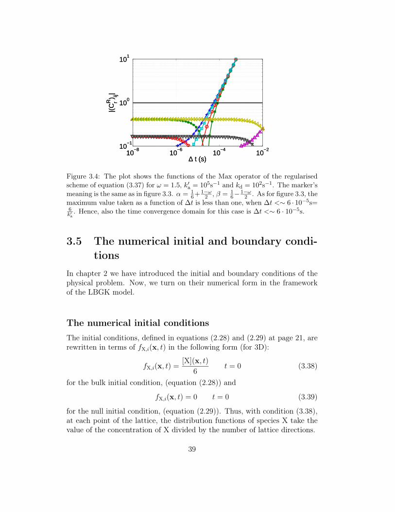
10−8

10−6

10−4

10−210

−1

100

101

∆ t (s)

|(C

rR) ij|

10−8

10−6

10−4

10−210

−1

100

101

∆ t (s)

|(C

rR) ij|

Figure 3.4: The plot shows the functions of the Max operator of the regularisedscheme of equation (3.37) for ω = 1.5, k′

a = 105s−1 and kd = 102s−1. The marker’smeaning is the same as in figure 3.3. α = 1

6+ 1−ω2 , β = 1

6− 1−ω2 . As for figure 3.3, the

maximum value taken as a function of ∆t is less than one, when ∆t <∼ 6 · 10−5s=6k′

a. Hence, also the time convergence domain for this case is ∆t <∼ 6 · 10−5s.

3.5 The numerical initial and boundary condi-

tions

In chapter 2 we have introduced the initial and boundary conditions of thephysical problem. Now, we turn on their numerical form in the frameworkof the LBGK model.

The numerical initial conditions

The initial conditions, defined in equations (2.28) and (2.29) at page 21, arerewritten in terms of fX,i(x, t) in the following form (for 3D):

fX,i(x, t) =[X](x, t)

6t = 0 (3.38)

for the bulk initial condition, (equation (2.28)) and

fX,i(x, t) = 0 t = 0 (3.39)

for the null initial condition, (equation (2.29)). Thus, with condition (3.38),at each point of the lattice, the distribution functions of species X take thevalue of the concentration of X divided by the number of lattice directions.

39

The numerical boundary conditions

The numerical boundary conditions are written by using either the formulasshown in proposition 3 in appendix A

fX,i(x, t) = f eqX,i(x, t) + f

(1)X,i (3.40)

if we want to recover a Neumann boundary condition, i.e. the flux is known,or the simple formula

fX,i(x, t) = [X](x, t) −∑

j 6=i

fX,j(x, t) (3.41)

which give the fX,i(x, t) as a function of the [X](x, t) and the fX,j with j 6= i.The numerical form of the boundary conditions are listed below.

Solution side: finite Diffusion

The boundary condition of finite diffusion stated in equation (2.30) is

fX,i(x, t) = [X]∗ −∑

j 6=i

fX,j(x, t) |x| = d (3.42)

where d is the distance of diffusion, the lhs is the missing value and the rhs isknown. This equation is equivalent, as already said in the previous chapter,to have a stirred solution at distance d from the consuming surface.

Solution side: semi-infinite Diffusion

The boundary condition of semi-infinite diffusion is similar to the previousboundary condition of finite diffusion with the difference that the finite dif-fusion length d should be at least 5 times of the diffusion layer thicknessδ =

√

(πDMt). This condition ensures that the diffusion process is not af-fected by the boundary at distance d. Therefore the semi-infinite diffusioncondition is

fX,i(x, t) = [X](x, t) −∑

j 6=i

fX,j(x, t) |x| = 5δX (3.43)

where fX,i(x, t) is the missing value and the rhs is known.

40

Flux boundary condition at interface

A flux boundary condition means that the concentration gradient at thesurface along the normal vector n must be defined or computed. When thesurface is not regular and does not match the lattice, such computation isnot trivial. However, a good approximation is to discretize the surface withlattice points with a sufficient small grid size and compute the flux at theboundary at the closest lattice points outside the surface. In this way thesurface is approximated by a collection of step functions, which in the limitof small grid size, takes the same shape as the surface boundary. Therefore,the cubic nature of the lattice is preserved and equation (3.20) can be used.As an example of application let us consider the simple 1D planar problem.The boundary conditions for L and ML, at x = 0 are

fL,1 = fL,3 (3.44)

fML,1 = fML,3 (3.45)

Nernst and flux boundary condition at interface

Nernst boundary condition apply when the consuming surface is a voltam-metric electrode on which the metal ion M is reversibly reduced into M0.Again, to obtain the numerical boundary condition at x = 0, for M and M0,conditions (2.35) and (2.36) must be transformed in terms of density distri-bution functions. By combining expression (3.41) with the Nernst condition(2.35) and equation (3.41) with the flux conservation, eqn (2.36) to write thegradient, it is possible to find two equations with two unknowns along eachCartesian axis. For instance, along the x axis, one gets:

fM,1 + fM,3 = (fM0,1 + fM0,3)e(E−E0)nf (3.46)

βM(fM,1 − fM,3) = β0M(fM0,1 − fM0,3) (3.47)

where n is the number of electrons, f is the Faraday reduced constant,βM = ωMDM

∆xand βM0 =

ωM0DM0

∆x0, ∆x and ∆x0 are the mesh sizes of the

space in solution and inside the electrode, respectively. After some algebraicmanipulation one gets:

fM0,3 =fM0,1(β

0M − βMe(E−E0)nf ) + 2fM,3βM

βMe(E−E0)nf + β0M

(3.48)

fM,1 = (fM0,1 + fM0,3)e(E−E0)nf − fM,3 (3.49)

In most of the applications discussed in this thesis, cases where E ¿ E0,are considered, so that the electrode surface is a perfect sink for M. Under

41

such conditions, we do not need to compute the concentration of M0 andthe conditions stated by the previous equations (3.48) and (3.49) can besimplified to a condition only on M

fM,1 = −fM,3

The Michaelis-Menten condition at interface

In section 2.4.3 we have described the Michaelis-Menten condition in thecomplete form, equation (2.38) at page 23. In this thesis we use the steady-state approximation, equation (2.39) at page 23:

Jint =1

A

dN

dt=

kintKaRtot[M]

1 + Ka[M]x ∈ S (3.50)

In this approximation the Michaelis-Menten condition becomes a mixed bound-ary condition. Therefore we can apply the equation (3.40) to the equation(3.50) and the numerical condition is rewritten along the Cartesian directionsas

Jx =ωdD

∆x(f

(1)1 − f

(1)2 )

Jy =ωdD

∆x(f

(1)3 − f

(1)4 )

Jz =ωdD

∆x(f

(1)5 − f

(1)6 )

(3.51)

where Jx, Jy and Jz are the x, y and z components of the internalisationflux.For instance, for a planar surface, if Ka[M] ¿ 1 as it is often the case fortrace metal, the Michaelis-Menten numerical boundary condition, reduces tosolve the following algebraic equation in the unknown fM,1:

2ωMDM

∆x

(

fM,1 − fM,2

)

= kintKaRtot

(

fM,1 + fM,2

)

from which, after simple computations, one get:

fM,1 = −1 + 2ωMDM

kintKaRtot

1 − 2ωMDM

kintKaRtot

fM,2 (3.52)

Following the same reasoning, but with more calculation, one can extendthe above condition for 3D spherical surface, by discretizing the surface withelementary cubes of size ∆x.

42

3.6 Summary

In this chapter, after having reviewed the basics of the LB approach, a newregularised LBGK scheme was suggested to discretize and numerically solvethe reaction-diffusion problem stated in equations (2.24), (2.25), (2.26) and(2.27) of chapter 2. We have shown that, considering typical real values ofthe chemical rate constants, the regularised LBGK scheme converges fasterthan the standard LBGK scheme and that it has also a larger convergencedomain. Finally, the numerically counterpart of the initial and boundaryconditions was given. We believe that the Nernst + Flux balance boundarycondition and the Michaelis-Menten equation have never been treated beforein the LBGK framework.

43

Chapter 4

The Multi-scale Methods: TimeSplitting and Grid Refinement

4.1 Overview

As we have seen in the previous chapters, we are facing a problem with spaceand time scales that vary over a large range of magnitude.This class of problems are called multiscale problems. In the literature manyauthors have investigated these problems, by using different numerical meth-ods, see for instance [61, 62, 63, 64, 65, 66].In the framework of the Lattice Boltzmann schemes, authors have focustheir attentions to study the different time scales of a problem by applyingmulti-block schemes [67, 68] or multi-components schemes [36, 27, 69]. How-ever, the combined use of the time splitting method and the grid refinementtechniques in the framework of the Lattice Boltzmann scheme for reaction-diffusion has never been used at the present time to simulate chemical andphysical heterogeneous complex systems.The chapter is organised as follows. Section 4.2 is devoted to the time split-ting method. It is organised in three parts. In the first part, the basics ofthe time splitting method are given. In the second part, its application tothe Lattice Boltzmann framework is described for reaction-diffusion problemand, in the third part, the method is validated with some benchmarks.Section 4.3 is devoted to the grid refinement methods. It is organised asfollows. We start to give the reason to refine the grid, then we describe indetail three grid refinement techniques in the Lattice Boltzmann framework,focusing on one dimensional geometries. Then, they are validated with somebenchmarks.Finally in section 4.4, we state the numerical algorithm we use and we give a

45

complete description of the numerical scheme by applying it to the prototypeproblem.

4.2 The Time splitting Method

4.2.1 Introduction

The time splitting method is a classical technique, first introduced by Ya-nenko [70], to solve problems involving several physical and chemical pro-cesses taking place at different time scales with widely different rate con-stants. A good introduction of this method can be found in [23].As mentioned above, the presence of several physical and chemical processesis a major feature of environmental and biological systems. Many authorshave already applied splitting methods to reaction-diffusion systems [71],where different time scales need to be resolved, and to dynamic systems[23, 72] where a suitable statistical description of the phenomena is requiredfor the large number of unknowns involved. To our knowledge the time split-ting technique has never been coupled to the regularised LBGK approach.The numerical scheme previously defined in equation (3.7) is second orderaccurate 1 and valid only when, as we have shown in section 3.4, the timestep of integration ∆t is sufficiently small with respect to the association-dissociation reaction times. This limitation, cannot be avoided by explicitschemes: solving fast problem requires to reduce the time step of integrationto keep the error bound. However, when two processes take place at differenttime scales, the problem can be reformulated in a more convenient way. Inparticular, one can discriminate two different time scales: the time scale ofdiffusion and that of reaction.For instance, regarding the prototype problem (2.3), our purpose is to per-form simulations in a wide range of values of the (pseudo) first order rateconstants kacL and kd, typically between 10−5s−1 and 108s−1, with usuallyK ′ = kacL

kdÀ 1, i.e. under conditions where the complex has a major contri-

bution to the flux.Thus the reaction time scale, equation (2.13) ranges between ns and hours,while the time scale of diffusion, equation (2.14), is usually in the range fromms to s.Roughly speaking, the time splitting method is needed when the time scaleof reaction is much smaller than the time scale of diffusion, i.e. tR ¿ tD.For instance, let us consider a system with ka[L]∗ = 106s−1, δM = 10µmand DM = 10−10m2s−1. The reaction time tR is of the order of µs, while

1See appendix A

46

tD = δ2/DM = 1s. For equation (3.7) to be valid, the time step of integra-tion ∆t must be less than tR = 10−6s, whereas total time will be secondsto minutes. For a system with the same diffusion time but a faster reactionka[L]∗ = 108s−1, the time step of integration must be less than 10−8s, againfor a total time of seconds to minutes. Such a low value of integration time isnot reasonable due to the very high computational CPU time required and,so, another method such as the time splitting is needed to overcome thisdifficulty.

4.2.2 The basics of the time splitting method

We will outline below a numerical scheme which makes use of the time split-ting method within the framework of the regularised LBGK scheme (3.7).The idea of the splitting method is to solve separately the diffusion and thereaction parts. This will produce extra integration errors, but will allow usto deal efficiently with a large difference in the characteristic time scales.For simplicity, we shall illustrate the splitting technique directly at the levelof the partial differential equations so as to build two coupled problems.Let c be the vector of concentration functions 2. The original problem is

∂c

∂t= TDc + TRc (4.1)

where TD and TR are the diffusion and the reaction operators, respectively.With appropriate choices of TD and TR, our problem stated in equations(2.4)-(2.7) can be easily recovered.We want to compute the concentration c at time t+∆t, c(t+∆t), by solvingthe equation (4.1) on the time domain (t, t + ∆t] with the initial conditionat time t, c(t) = ct. By using the standard time splitting method, equation(4.1) is decomposed into

∂c′

∂t= TDc′ on (t, t + ∆t] with c′(t) = ct (4.2)

∂c′′

∂t= TRc′′ on (t, t + ∆t] with c′′(t) = c′(t + ∆t) (4.3)

The final value is c(t + ∆t) = c′′(t + ∆t). This decomposition is also calledRD scheme, because the diffusion operator TD is solved at the first step andthe reaction operator TR is solved at the second step.

2Following the standard mathematical notation, the vector function c is introduced.Each entry of it contains the concentration function of each species. For instance, consid-ering the prototype problem, equation (2.3), X=M, L and ML, hence c = (cM, cL, cML)T.

47

It can be shown [23] that the time splitting scheme is exact if the reactive andthe diffusive operators commute. If they do not commute, the time splittingerror is accurate at the second order in space and at least first order in time.

4.2.3 The time splitting method in the LBGK frame-work

Principles explained with the RD mode

We will consider two LB dynamics to solve the coupled system of equations(4.2) and (4.3), one for each process. The first equation is solved by applyingthe pure diffusive dynamics:

fX,i(x + vi∆t, t + ∆t) = fX,i(x, t) + ΩNRX,i (x, t)

The second equation is solved by applying the pure reactive dynamics:

fX,i(x, t + ∆t) = fX,i(x, t) + ΩRX,i(x, t)

The pure diffusive scheme is non-local and it can be decomposed into itscollision and propagation parts 3. On the other hand the second scheme ispurely local and it reduces only to one collision step.The idea is to perform the diffusive collision, followed by the reactive collisionand, finally, by the propagation.Therefore, by using the RD splitting scheme, the complete numerical scheme(3.7) is now split into its pure diffusive and reactive parts as (figure 4.1, left):

fX,i(x, t′) = fX,i(x, t) + ΩNRX,i (x, t) (t, t′] (4.4)

fX,i(x, t′′) = fX,i(x, t′) + ΩRX,i(x, t′) (t′, t′′] (4.5)

fX,i(x + vi∆t, t + ∆t) = fX,i(x, t′′) t′′ = t + ∆t (4.6)

3Notice that the decomposition into collision and propagation steps of whatever LatticeBoltzmann dynamics, can be considered as an application of the time splitting scheme tothe original Boltzmann equation. In fact, it can be shown that the Lattice Boltzmannscheme, in its LBGK approximation, is equivalent to the discretization of the BoltzmannEquation in the BGK approximation

∂f

∂t+ v · ∇f = ω(f eq − f)

by applying the time splitting method to separate the streaming operator v · ∇f from thecollision operator ω(f eq − f).

48

Here we have assumed that the time variable t′ for the diffusion equationruns differently from the time variable t′′ of the reaction equation. In fact,the difficult problems to handle are those where the reaction time run fasterthan the diffusion time, i.e. tr ¿ td. These class of problems, where reactionis fast, are also known in literature as stiff problems.A schematic description of the RD scheme is shown in the left hand sideof figure 4.1. The sub-problem (4.4) is a numerical initial-boundary-value

Figure 4.1: Example of RD, DR and DRD splittings.

problem involving only diffusion process, therefore it will be called processD. On the other hand, sub-problem (4.5) is a numerical initial value probleminvolving only a chemical reaction, therefore it will be called process R. Insuch a way, we can define several splitting procedures.Notice that process R, as expressed in equation (4.5) is an explicit scheme,because the values of ΩX,i(x, t) are computed at the actual time level. How-ever, the very advantage of the time splitting method, is the possibility ofusing different techniques for sub-problems (4.4) and (4.5) and to use differ-ent time integration steps. In fact, during the simulation the time step ∆thas to be understood as the main integration time and when not explicitlyspecified it will be used for both schemes D and R. Furthermore, to takeadvantage of the splitting techniques, an implicit scheme, which warrants alarger stability region [73], should be used for the reaction process (4.5). Inthis case, equation (4.5), is replaced with:

fX,i(x, t′′) = fX,i(x, t′) + ΩRX,i(x, t′′) (4.7)

We discuss quantitatively the advantages of the time splitting for fast chem-ical reactions in section 4.2.4 where the four splittings, discussed below, are

49

validated. Before beginning this discussion, three other splitting modes (DR,DRD and RDR) are explained steps by step below.

DR splitting

The DR splitting mode is defined in the same way as the RD mode. (see themiddle of figure 4.1) by interchanging equation (4.4) with equation (4.5). Inthe time interval [t, t′ = t + ∆t], firstly we compute an intermediate functionfX,i(x, t′) by solving equation (4.5) (where t′ is replaced by t and t′′ is replacedwith t′), with initial condition fX,i(x, t). Then, in the same time interval,[t′ = t, t′′ = t + ∆t], we compute fX,i(x, t′′) by solving equation (4.4) (byreplacing t with t′ and t′ with t′′), with the initial condition fX,i(x, t′) and theappropriate boundary conditions. Finally the solution at t + ∆t is obtainedby applying equation (4.6). The complete numerical RD scheme is thus:

fX,i(x, t′) = fX,i(x, t) + ΩRX,i(x, t) (t, t′] (4.8)

fX,i(x, t′′) = fX,i(x, t) + ΩNRX,i (x, t′) (t′, t′′] (4.9)

fX,i(x + vi∆t, t + ∆t) = fX,i(x, t′′) t′′ = t + ∆t (4.10)

DRD splitting

DRD splitting is defined as follows (see the right side of figure 4.1): in thetime interval [t, t′ = t+∆t/2] firstly we compute an intermediate function bysolving the equation (4.4) with the appropriate boundary conditions and theinitial condition fX,i(x, t). Then, in the time interval [t′ = t, t′′ = t + ∆t], wecompute another intermediate function by solving the equation (4.5) withthe initial condition fX,i(x, t′). Finally, we compute a third intermediatefunction at t′′′ = t+∆t by solving again the equation (4.4) in the time interval[t′′ = t+∆t/2, t′′′ = t+∆t] with the appropriate boundary conditions and theinitial condition fX,i(x, t′′). The solution at time t + ∆t is finally computedby applying equation (4.6). The splitting mode RDR is deduced in the sameway, with the role of R and D exchanged. The complete numerical DRDscheme is given below:

fX,i(x, t′) = fX,i(x, t) + ΩNRX,i (x, t) (t, t′] (4.11)

fX,i(x, t′′) = fX,i(x, t) + ΩRX,i(x, t′) (t′, t′′] (4.12)

fX,i(x, t′′′) = fX,i(x, t′′) + ΩNRX,i (x, t′′) (t′′, t′′′] (4.13)

fX,i(x + vi∆t, t + ∆t) = fX,i(x, t′′′) t′′′ = t + ∆t (4.14)

50

4.2.4 Time splitting validation

Several tests has been made to check the capability and the accuracy of thevarious splitting modes. Here we give the most important results that allowedus to choose the RD splitting as the most convenient for our purposes. Fromnow on, we indicate with NS the non splitting scheme, i.e. the original LatticeBoltzmann scheme for reaction-diffusion in its standard version, equation(3.7).We consider the planar semi-infinite diffusion-reaction prototype problem(2.3) stated in equation (2.4) - (2.6), defined on the interval (0, +∞), wherethe consuming surface is placed at x = 0, with the following initial andboundary conditions: cX(x, 0) = c∗X, cX(x → +∞, t) = c∗X for X=M,L andML, cM(0, t) = 0 and both ML and L have nil flux at x = 0. We distinguishtwo time step of integrations: ∆tD and ∆tR which are the time step ofreaction and diffusion, respectively. In all plots the same step size was usedfor diffusion and reaction, i.e. ∆tD = ∆tR.Figure 4.2 shows that the absolute l2-error, defined as

‖cM(x, t) − uM(x, t)‖2 =

√

√

√

√

n∑

j=1

|cM(xj, t) − uM(xj, t)|2 (4.15)

where uM is the analytical solution and n the number of lattice points,decreases with the number of iteration steps with a slope approximatelyequal to -1, indicating a first order convergence, up to 1000 iteration steps,for the non-splitting scheme and all the splitting schemes. In general, wecan say that all the schemes are sufficiently accurate with approximately thesame absolute precision.The error on flux computation, JM, at a consuming surface, is defined as

εr =|JM − Je|

Je

(4.16)

where Je is the exact solution, either for the inert case or for the fully labilecase (see equations (2.15) and 2.16). εr depends on ∆t

∆xand on the equilibrium

constant K, as shown in Figure 4.3. The numerical scheme associated withthe reaction is solved by an explicit method. In all plots we observe thatthe NS scheme is the most accurate and, within the splitting schemes, RDis the best. Furthermore, we observe that when K takes high values, K >1000m3mol−1, then the NS scheme no longer converges and we have to usethe splitting schemes.Table 4.1 reports results obtained with RD and NS methods for the flux

at t = 0.5s. They are compared with the exact solution given in [74] for a

51

102

103

10410

−7

10−6

10−5

t / ∆ t

L 2 err

or

slope = −1 NS

RD

DR

DRD

RDR

Figure 4.2: Error in the l2-norm on the concentration profile of M vs the numberof iteration steps. (NS is the standard scheme without splitting.) The diffusioncoefficient are all equal to 10−9m2s−1, K ′ = K[L]∗ = 0.1, kd = 10−7s−1, ka =10−8molm−3s−1, t = 1ms, ∆x = 10−6m, n = 201, [M]tot = 10−3molm−3 and[L]tot = 1molm−3. A reference slope of -1 has been added to compare the numericalschemes. The splittings are solved using the same integration time steps for thediffusion and the reaction schemes. Markers for NS and RD on one hand and DRand RDR on the other hand are indistinguishable in the plot, because they givealmost the same error.

kd (s−1) RD NS Exact10−5 0.09096 0.09093 0.0909110−4 0.09101 0.09098 0.0909510−3 0.09141 0.09138 0.0913610−2 0.09545 0.09543 0.0954110−1 0.13196 0.13195 0.13194

1 0.31929 0.31949 0.3195410 0.66661 0.66792 0.66867102 0.91865 0.92330 0.92660103 0.98150 0.98113 0.99114104 0.98828 Not convergent 0.99909105 0.98828 Not convergent 0.99991

Table 4.1: Normalised flux results of numerical simulations with the followingparameters: K ′ = K[L]∗ = 10, DM = DML = 10−9m2s−1, t = 0, 5s, ∆x = 10−6m,∆tD = 0.1ms, ∆tR = 50µs, [M]tot = 10−3molm−3, [L]∗ = 1molm−3 and n = 201.

52

101

102

10310

−10

10−5

100

ε rel

101

102

10310

−5

100

∆ t / ∆ x (s/m)

ε rel

∆ t / ∆ x (s/m)

101

102

10310

−4

10−2

100

∆ t / ∆ x (s/m)

ε rel

∆ t / ∆ x (s/m)10

110

210

310−4

10−2

100

ε rel

A B

C D

Figure 4.3: Relative error on the flux at t = 0.1 seconds, computed for severalequilibrium constants as a function of the ratio ∆t

∆x , in excess of ligand condition.All the diffusion coefficients take the same value as for table 4.2, [L]∗ = 1molm−3

and kd = 1s−1. The number of iteration steps is 1000 in all the simulations. PlotA: K = 10m3mol−1, plot B: K = 100m3mol−1, plot C: K = 1000m3mol−1 andplot D: K = 10000m3mol−1. Same markers as in figure 4.2. The RD scheme,compared with the others splitting schemes seems to be the best splitting schemes,in all cases.

53

wide range of dissociation rate constants, kd. At low or intermediate valuesof kd, both numerical schemes show a good agreement with the exact values,but when kd becomes too large then the NS scheme fails to converge, whilethe RD splitting continues to give good results close to the exact ones. Thenumerical results obtained by the RD method, however, do not convergecompletely to the exact values. In table 4.1 the last two values, correspondingto kd = 104s−1 and kd = 105s−1 differ from the exact value by ∼ 6%. Thisdiscrepancy is due to the very small reaction layer thickness µ < 0.1µm,compared to the space mesh ∆x = 1µm. Indeed, in order to follow thevariation of the concentration profiles, inside this layer, the mesh size ∆xhas to be of the same order of magnitude of µ or smaller. This is not thecase for the results discussed above, where ∆x > µ, for the largest kd values.Table 4.2 shows the computational costs of the different splitting procedures.

RD DR DRD RDRExplicit 1 1 1.1 1.8Implicit 5.3 5.3 5.4 10.4

Table 4.2: Relative computational costs normalised with respect to the explicit RDscheme. RD explicit simulations take about 4 seconds on a Pentium 4 to perform1000 iteration steps in a lattice with 1000 points.

The results shown in Table 4.2 and the better accuracy exhibited in general bythe RD scheme for computing the flux, suggest that this scheme is the mostappropriate numerical procedure for our purpose. Specifically, considering1000 iterations, in a grid with 1000 points, with ∆tD = ∆tR on a Pentium 4(CPU 2.80 Ghz), the explicit RD and DR schemes take about 4 seconds, theexplicit DRD and RDR take about 6 seconds and the non splitting schemetakes about 3 seconds. Table 4.2 also show that the implicit scheme, equation(4.7), takes always much more than the explicit scheme. For that reason, inthe rest of the thesis, we always work with an explicit scheme.Figure 4.4 shows the behaviour of the relative error on the flux, as a functionof the ratio ∆x

µand of the equilibrium constant K ′ = K[L]∗. It enables us to

choose the conditions under which this error is minimised. The simulationshave been performed with the RD scheme. When the contribution of thecomplex to the flux becomes important (K ′ > 1) the error is negligible (orderof a few percent) if ∆x < µ. By comparing the degree of accuracy and thecomputational effort with the others three modes (DR, DRD and RDR), theRD scheme is the more convenient splitting scheme.

54

100

102

104

10−1

100

101

10−4

10−3

10−2

10−1

100

ka c

L / k

d∆ x / µ

ε rel

Figure 4.4: Plot of the error on the flux after 1000 time step iterations as a functionof K ′ = K[L]∗ and of the ratio ∆x

µ . Computation with the RD scheme. kd =

100s−1, diffusion coefficients for all the species equal to 10−10m2s−1. We see thatfor significant contribution of the complex (i.e. when K ′ > 1), the error is negligible(less than 1%) for ∆x < µ.

55

4.3 The Grid Refinement Methods

Grid refinement (GR) is a technique in which the computational mesh is madefiner in the regions where small scale processes take place, while to save CPUtime and memory, a coarser grid is used in less demanding regions. Manystrategies have been developed in the implementation of different GR in theLattice Boltzmann approach, see for instance [37, 24, 75]. Many theoreticalstudies, the so-called adaptative grid [76, 77, 78, 49], involves the investiga-tion of the correct grid size to use in these layers when they become thin.There are clearly two opposite constraints. If the fine grid spans a large partof the computational domain, the numerical solution will be more accurate,but the CPU time and memory usage may increase beyond acceptable limits.The question is then to know how to divide in an efficient way the domainin coarse and fine grids. Note that, obviously, there can be more than twogrid levels. Another question is to determine the most appropriate change ofmesh size between two adjacent grids as well as the best way to couple thephysical quantities on both side of the grid interface.The goal of this section is to propose three new ways of coupling grids ofdifferent mesh size in the context of an LB solver for reaction-diffusion pro-cesses. Before explaining them in detail, it is interesting to give a quantitativereason about the need to refine the grid.

4.3.1 The reason to refine the grid

Let us consider a simple diffusion problem with only one species, say M, andlet us vary its reaction rate of formation, say k. We consider a 1D problemin a semi-infinite domain (0, +∞), with initial condition

[M] = [M]∗

boundary semi-infinite diffusion condition

[M] → [M]∗ x → +∞

and perfect sink condition

[M] = 0 x = 0

The time splitting exact solution (equation (4.2) and (4.3)) in the time in-terval [0, t] is [23]:

[M] = [M]∗ekterf( x

2√

DMt

)

(4.17)

56

If we consider the exact solution in two points, say x and x + ∆x, we canwrite:

cM(x + ∆x, t) − cM(x, t) = c∗Mekt[

erf(x + ∆x

2√

DMt

)

− erf( x

2√

DMt

)]

(4.18)

The first order Taylor series expansion around x of an amount ∆x, with∆x → 0, allows us to write:

cM(x + ∆x, t) − cM(x, t) = c∗Mekt∆xe− x2

2√

DMt

√πDMt

(4.19)

In general, we expect that [M] will vary continuously to ensure numericallyaccuracy. So, if we require that |cM(x+∆x,t)−cM(x,t)|

c∗M< θ, then we obtain the

condition:

∆x < e−kt√

πDMtex2

2√

DMt · θ (4.20)

Inequality (4.20) says that: a) ∆x has an upperbound and b) if we considertwo rates k1 and k2 such that k1 > k2, then ∆xk1 < ∆xk2 . Therefore, forvery fast reaction dynamics, in order to get a variation between x and x+∆xless than θ, the grid size ∆x has to be chosen small enough, accordingly withinequality (4.20).Furthermore, it is not necessary to use the inequality (4.20) in all the domain.It is advisable to restrict its usage only to region where this is really needed,i.e. close to the consuming surface and, more precisely, within the regioncomparable to the reaction layer thickness, µ, equation (2.12).

4.3.2 The grid refinement schemes

Grid refinement amounts to using different grid spacing along the computa-tional domain Ω. Such a choice is necessary when large variations of massoccur in Ω. This is the case, for instance, when ka value is large, i.e. when thereaction layer thickness µML, equation (2.12) at page 16, is between 10−9mand 10−6m. In this region it is necessary to set grid sizes less than the reac-tion layer thickness.However, not in all the domain it is required to have small grid sizes. Hence,we divide the domain Ω into s sub-grids G1,. . .,Gs, such that Ω = G1∪. . .∪Gs.Each sub-grid is made by ni points, such that the total number of pointsnx =

∑si=1(ni − 1) + 1. The Gi are discretized in time with a time step ∆ti

and in space with a grid size ∆xi, such that ∆xi+1 > ∆xi. In order to make asimple but sufficiently general description, we choose to divide the domain inthree sub-grids, i.e. we put s = 3, even though for real computations, s can

57

be larger. In chapter 6, we show several applications to real environmentalsystems, in the planar approximation, where the number of sub-grids variesfrom s = 2 up to s = 11 and their sizes are automatically chosen to discretizein the best way the whole domain.The set up of the grid is illustrated in Fig. 4.5. Points A and D are bound-

Figure 4.5: Set up of a 1D computational domain with three sub-grids Gi, i =1, 2, 3. Circle, rhombus and square markers represent points belonging to G1, G2

and G3 respectively.

ary points, while points B and C are sub-grid interface points of G1-G2 andG2-G3 respectively. Notice that points B and C belong to both adjacentsub-grids.At the first step, we have to choose the smaller grid size, ∆x1. As mentionedabove, it should be smaller than the smallest reaction layer thickness. Sec-ondly, we chose the smaller time step, ∆t1. In order to satisfy convergenceconditions, equation (3.33) page 35, ∆t1 must be smaller than the smallesttime scale of the process, usually ∆t1 <Minij(

jka,i[jL])−1. The total number

of points, nx, the number of point of G1, n1 and the length of the domain, lare chosen arbitrarily.Let us define, here, the density distribution functions fX,i of the LB methodat each sub-grid, which will be useful in the rest of the section to describethe grid refinement methods. Let f

(Gk)X,i (xj ∈ Gk, t) for j = 1, . . . , nk be the

density functions of each species X at the points of sub-grid Gk for k = 1, 2, 3.Points B and C are critical, because, at these points, not all the density dis-tribution functions are computed by the numerical scheme. Some of themremain unknowns and need to be estimated invoking either 1) time interpo-lation or 2) conservation of mass and flux.Time interpolation is performed whenever we need to compute a functionwhich cannot be computed with the evolution equation. For instance, let ussuppose that in G2 ∆t2 = 2∆t1. The function f

(G1)X,2 (B, t + ∆t1) is not known

and to compute it, we interpolate from the corresponding functions alreadycomputed in the sub-grid G2, for instance by using a first order interpolationin time, f

(G1)X,2 (B, t + ∆t1) = 1

2(f

(G2)X,2 (B, t − ∆t1) + f

(G2)X,2 (B, t + 2∆t1)).

58

The condition of conservation of mass and flux only works for the special1D case. A complete detailed explanation of it can be found in [79]. Such acondition, which will be called "grid interface condition", in terms of densitydistribution functions, e.g at the point B, reads:

f(G1)X,1 (B, t) + f

(G1)X,2 (B, t) = f

(G2)X,1 (B, t) + f

(G2)X,2 (B, t) (4.21)

ω1

∆x1

(f(G1)X,1 (B, t) − f

(G1)X,2 (B, t)) =

ω2

∆x2

(f(G2)X,1 (B, t) − f

(G2)X,2 (B, t))(4.22)

where f(G2)X,1 (B, t) and f

(G1)X,2 (B, t) are the unknowns, while f

(G2)X,2 (B, t) and

f(G1)X,1 (B, t) are computed from the evolution scheme 4. The first equation in

the set (4.21) is the conservation of mass

[X](G1)(B, t) = [X](G2)(B, t)

while the second equation is the conservation of flux

J(G1)X (B, t) = J

(G2)X (B, t)

Based on this principles, we propose 3 schemes for grid refinement (S1, S2

and S3)

Grid refinement S1 - Constant lattice velocity

In this method, we fix the lattice velocities at constant value in all the sub-grids:

∆xi

∆ti= constant i = 1, 2, 3 (4.23)

Since we have already chosen the values of ∆x1 and ∆t1, the constant in theabove equation (4.23) is fixed to be some real number. On the other hand,the ratios ∆t2/∆t1 and ∆t3/∆t2 have to be integer numbers. For simplicity,we have chosen, i.e. ∆t2/∆t1 = ∆t3/∆t2 = 2, and ∆t3 is the largest time stepvalue. The complete numerical scheme during the time interval [t, t+ ∆t3] isshown in Algorithm 1 at page 60.

4Note that, the above "grid interface condition" works only for reactive-diffusiveschemes in 1D. For hydrodynamic problems and for diffusive 2D or 3D, our approachis not directly applicable, but we believe it is "equivalent" to the grid refinement proposedby [75] based on the conservation of the equilibrium functions and on the rescaling of thenon-equilibrium functions. The approach given in [75] is based on the fact that along thesub-grids, the conserved quantities does not depend on the lattice resolution but only onphysical quantities. Our approach follows the same line: with condition (4.21), we im-pose the same values to the physical quantities (mass concentration and flux) across thesub-grid interfaces.

59

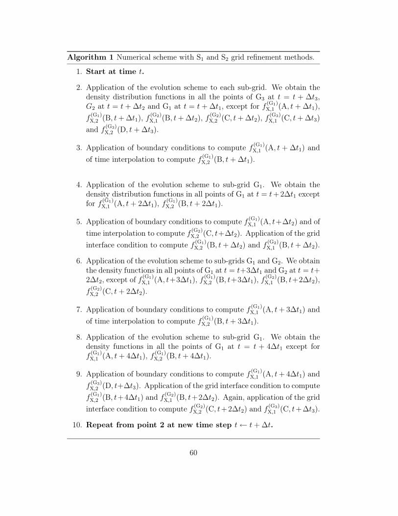
Algorithm 1 Numerical scheme with S1 and S2 grid refinement methods.

1. Start at time t.

2. Application of the evolution scheme to each sub-grid. We obtain thedensity distribution functions in all the points of G3 at t = t + ∆t3,G2 at t = t + ∆t2 and G1 at t = t + ∆t1, except for f

(G1)X,1 (A, t + ∆t1),

f(G1)X,2 (B, t + ∆t1), f

(G2)X,1 (B, t + ∆t2), f

(G2)X,2 (C, t + ∆t2), f

(G3)X,1 (C, t + ∆t3)

and f(G3)X,2 (D, t + ∆t3).

3. Application of boundary conditions to compute f(G1)X,1 (A, t + ∆t1) and

of time interpolation to compute f(G1)X,2 (B, t + ∆t1).

4. Application of the evolution scheme to sub-grid G1. We obtain thedensity distribution functions in all points of G1 at t = t+2∆t1 exceptfor f

(G1)X,1 (A, t + 2∆t1), f

(G1)X,2 (B, t + 2∆t1).

5. Application of boundary conditions to compute f(G1)X,1 (A, t+∆t2) and of

time interpolation to compute f(G2)X,2 (C, t+∆t2). Application of the grid

interface condition to compute f(G1)X,2 (B, t + ∆t2) and f

(G2)X,1 (B, t + ∆t2).

6. Application of the evolution scheme to sub-grids G1 and G2. We obtainthe density functions in all points of G1 at t = t+3∆t1 and G2 at t = t+2∆t2, except of f

(G1)X,1 (A, t+3∆t1), f

(G1)X,2 (B, t+3∆t1), f

(G2)X,1 (B, t+2∆t2),

f(G2)X,2 (C, t + 2∆t2).

7. Application of boundary conditions to compute f(G1)X,1 (A, t + 3∆t1) and

of time interpolation to compute f(G1)X,2 (B, t + 3∆t1).

8. Application of the evolution scheme to sub-grid G1. We obtain thedensity functions in all the points of G1 at t = t + 4∆t1 except forf

(G1)X,1 (A, t + 4∆t1), f

(G1)X,2 (B, t + 4∆t1).

9. Application of boundary conditions to compute f(G1)X,1 (A, t + 4∆t1) and

f(G3)X,2 (D, t+∆t3). Application of the grid interface condition to compute

f(G1)X,2 (B, t+4∆t1) and f

(G2)X,1 (B, t+2∆t2). Again, application of the grid

interface condition to compute f(G2)X,2 (C, t+2∆t2) and f

(G3)X,1 (C, t+∆t3).

10. Repeat from point 2 at new time step t ← t + ∆t.

60

Grid refinement S2 - Constant relaxation parameter

In this method the relaxation parameters is independent of the sub-grids:

∆x2i

∆ti= constant i = 1, 2, 3 (4.24)

The reason under the choice of condition (4.24) is related with the LatticeBoltzmann scheme. The numerical precision of this scheme mainly dependson the relaxation parameter ωX. Equation (3.9) at page 29 shows that ωX

depends on the diffusion coefficient and the ratio ∆x2/∆t. Thus, if ∆x2/∆tis constant, then ωX is also constant, in all the sub-grids, and we expect thenumerical scheme to be more stable and precise (by choosing the optimal ω).As for the S1 method, the time steps ∆ti are such that ∆t2/∆t1 = ∆t3/∆t2 =2. As a consequence, the numerical scheme during the time interval [t, t+∆t3]is the same as that in the S1 method. It is shown in Algorithm 1 at page 60.

Grid refinement S3 - Constant time step

In this method the time steps is maintained constant among the sub-grids:

∆ti = constant i = 1, 2, 3 (4.25)

As for methods S1 and S2, we choose ∆x1 and ∆t1. The big advantage ofthis method is the absence of constraints on the grid sizes ∆xi. This is a veryimportant and useful feature, only valid for 1D problem, because it allowsus to choose the grid spacing arbitrarily. The second great advantage is thatthe algorithm is much simpler than that previously defined for S1 and S2. Inparticular, points 2 to 9 can be avoided. In fact, the evolution scheme shouldonly be applied once at each sub-grid (point 2 of previous scheme). Then, theunknown density functions at the grid interface are formed by applying thegrid interface condition (point 9 of the previous scheme). Note that no timeinterpolation is required. Therefore this method has the great advantageof being simple and easy to write in a numerical code. The correspondingalgorithm is shown in Algorithm 2 at page 62.

4.3.3 Grid refinement validation

The purpose of this section is to compare the performance of the grid re-finement methods S1, S2 and S3 described in section 4.3.2 and point out theadvantages and disadvantages of them.

61

Algorithm 2 Numerical scheme with S3 grid refinement method.

1. Start at time t.

2. Application of the evolution scheme to each sub-grid. We obtain thedensity distribution functions in all the points of G3 at t = t + ∆t,G2 at t = t + ∆t and G1 at t = t + ∆t, except for f

(G1)X,1 (A, t + ∆t),

f(G1)X,2 (B, t + ∆t), f

(G2)X,1 (B, t + ∆t), f

(G2)X,2 (C, t + ∆t), f

(G3)X,1 (C, t + ∆t) and

f(G3)X,2 (D, t + ∆t).

3. Application of boundary conditions to compute f(G1)X,1 (A, t + ∆t) and

f(G3)X,2 (D, t+∆t). Application of the grid interface condition to compute

f(G1)X,2 (B, t + ∆t) and f

(G2)X,1 (B, t + ∆t). Again, application of the grid

interface condition to compute f(G2)X,2 (C, t + ∆t) and f

(G3)X,1 (C, t + ∆t).

4. Repeat from point 2 at new time step with t ← t + ∆t.

Diffusive case

The validation is done with a pure diffusive case on the 1D domain Ω = (0, l),for which the exact solution is known at each time: absence of reaction,ka = kd = 0, cM(x = 0, t) = 1, cM(x = l, t) = 0 and cM(x, t = 0) = 0. Thetransient error between the exact solution and ce

M and the numerical solutioncnM is defined as follows:

ε(t) = Supi=1,...,nx

∣

∣

∣

ceM(xi, t) − cn

M(xi, t)

ceM(xi, t)

∣

∣

∣(4.26)

where the transient solution is:

ceM(x, t) =

∑

i

erfc[ lx(1 − (1 − x/lx) + 2i)

2√

DMt

]

−∑

i

erfc[ lx(1 + (1 − x/lx) + 2i)

2√

DMt

]

(4.27)The diffusion coefficient is 10−10m2s−1. The following parameters are fixed:nx = 101, n1 = 21, ∆t1 = 10−4s and l = 100µm. Due to the constraints(4.23) and (4.24), not all the values of ∆x1 are permitted for the S1 andthe S2 methods. We found that a good value, acceptable in both grids is:∆x1 = 5.58 × 10−7m. With these parameters, we have run the simulationsand plotted the transient error defined in equation (4.26).Figure 4.6 shows that the transient errors, of each method, are very similar,except for an oscillation of the error of S3 in the first 50 time iterations.

62

However, as time goes on, and the steady state is approached, the error issimilar and decreases with the same slope.

10−2

10010

−2

10−1

100

101

102

t (s)

ε %

S1

S2

S3

Figure 4.6: Comparison of the error (equation (4.26)) as a function of time for S1,S2 and S3 methods. ∆t1 = 10−4s. The errors are practically equivalent. Note thatthe error of the S3 method is oscillating in the first 50 iterations.

It is interesting to compare the computational effort in terms of number ofpoint updates of each method. Table 4.3 shows the number of point updatesfor each method until a fixed tolerance on the error is reached. The numberof point updates is the number of times each point is updated with thenumerical scheme during nt iterations. With our choice of discretization, thenumber of site updates, for the S1 and S2 methods, are

nt(4n1 + 2n2 + n3)

while for the S3 method, are

nt(n1 + n2 + n3)

where nt is the number of time iterations of the outer time loop, nt = t/∆t3(t is the physical time of integration). As we can see from table 4.3, themethod requiring less computational effort to get the fixed tolerance is theS2 method, while the S3 method is the most onerous. From our test, we cansee that S3 is 1.5 times more time consuming than S1 and S1 is about 1.5times more time consuming than S2.As a summary of the validation, we can point out that the error, for all the

63

ε < 0.01% ε < 0.1% ε < 1%S1 2968446 319124 23465S2 2025576 215880 15960S3 4643652 492134 38625

Table 4.3: Comparison of the computational effort of each grid refinement method.The table shows the number of site updates necessary to get an error (equation(4.26)) less than 0.01%, 0.1% and 1% for each method. Our test shows that theless onerous is the S2 method.

three methods, decreases when the diffusion-reaction time increases and itis similar for each method, see figure 4.6. Furthermore, a comparison of theCPU computational effort shows that the S2 method is about 1.5 and 3 timesfaster than S1 and S3 respectively. On the other hand, the method S3 is verysimple to implement in an algorithm because no restriction is required forthe size of the sub-grids. Moreover, the S3 method does not require any timeinterpolation. A summary with the performances of S1, S2 and S3 is given intable 4.4.

Simplicity to code precision CPU computational effortS1 Not simple good ∼ 3·106 site updates

Time interpolation needed to get ε < 0.01%S2 Not simple good ∼ 2·106 site updates

Time interpolation needed to get ε < 0.01%S3 Very simple good ∼ 4.6·106 site updates

No time interpolation to get ε < 0.01%

Table 4.4: Summary of the performance of S1, S2 and S3 achieved from our test.

4.3.4 Good choice of grid parameters for a typical reac-tive systems.

Results for one chemical reaction

Considering the results obtained in the previous section 4.3.3, taking intoaccount the error and the simplicity of the algorithm, we use the methodS3. Therefore, the time step ∆t is the same for all the subgrids, and theimportant point is how a reactive system influences the choice of the gridsize ∆xi for each subgrid, Gi and the distance among each Gi.Our practical interest is to compute metal flux at the consuming surfacewhere the concentration values of the species are not at equilibrium. The

64

largest concentration gradients appear near the consuming surface and so thefirst subgrid, G1, must have the smallest grid size. Thus, it is very importantto fix the grid size of G1 first, and determine the optimum values of i) itslength, let us call it xs, and ii) the ratio with the second subgrid G2, ∆x2

∆x1, in

order to obtain both a good precision and to save as much computation timeas possible in any complicated system.It is not easy to answer this question unambiguously. However, the resultsshow that some guidelines can be obtained, by plotting the error at a specifictime as a function of ∆x2

∆x1and xs/µ for the same problem, where µ is the

reaction layer thickness of the reaction M+L®ML.In the literature, the ratio ∆x2

∆x1is called grid refinement factor and below it

is denoted with g.Figure 4.7 shows the error contours for several values of xs/µ and g forthe limiting value of K = 1000m3mol−1 by applying the S3 scheme. Wehave computed the relative percentage error, with [L]∗tot = 1molm−3. Theassociation rate constant was fixed at ka = 1000m3mol−1s−1 to get the samevalue of the reaction layer thickness, µ ∼ 0.32µm. We observe that, if xs/µ <1 the error is not negligible and it increases taking values larger than 5 percentwhen xs/µ << 1. On the other hand, considering the region xs ≥ µ, whichis the more important for the applications, we observe that the method isgood, allowing us to obtain very low errors at large g values. For instance,for xs = µ, to get an error less than 2 percent, the values of g should be lessthan 5.Furthermore, figure 4.8 shows the gain in computer computation time as afunction of g, by using the same parameters of figure 4.7, but xs = µ. Thecurve shows that:

• The computation time decreases by a factor 2 for values of g between2 and 5 and it does not significantly change for g > 5.

• The error remains less than the acceptable threshold of 5%, increasingfrom ∼ 1% to ∼ 3% when g increases from 2 to 10.

In conclusion, for the reaction studied, which is a typical reaction in environ-mental systems, we have obtained that: i) the interface between the subgridsshould be placed at a distance larger or equal than the reaction layer thick-ness and ii) the grid refinement factor should be chosen in the reasonableinterval between 2 and 5 to get error on the flux computations less than 5%.

Generalisation to a mixture with nl ligands

In this section, we generalise the conclusions obtained above to set up thegrid refinement parameters, for reactive systems with nl ligands.

65

2 4 6 8 1010

−1

100

101

g

x s/µ 1

1

2

2

3

3

4

4

5

5

6

6

7

7

8

8

9

9

10 2

4

6

8

Figure 4.7: Relative percentage error contours, εr, given by equation (4.26), vsg and xs/µ for K[L]∗tot = 1000 for the grid refinement method, S3. Parameters:∆x1 = µ/20, ∆t1 = 0.01 · (ka[L]∗)−1, DM = DL = DML = 10−10m2s−1, ka = 1000m3mol−1s−1, kd = 1 s−1, t = 0.25s.

2 4 6 8 100.5

1

1.5

2

2.5

g

com

puta

tion

time

(min

utes

)

xs=µ

1.18%

1.75%

1.90%

2.02%2.29%

2.55%

2.80%

3.05%

3.29%

Figure 4.8: Computation time as function of the grid refinement factor g. Param-eters are the same as in figure 4.7, with xs = µ. The values near the curves are theerrors εr computed by using equation (4.26).

66

First, let us consider two reactions 1) M+1L­M1L and 2) M+2L­M2L. Theprocedure is split in three steps:

1. There are two reaction layer thicknesses, µM1L and µM2L, respectivelyassociate to the first and the second reaction. For accuracy reasons,we impose that the smallest grid size should be such that ∆x1 <Min(µM1L, µM2L).

2. As discussed in section above (see figure 4.7), we set two positions x1

and x2 such that µM1L < x1 < 3µM1L and µM2L < x2 < 3µM2L. IfµM1L < µM2L, then it is possible to choose x1 and x2 such that x1 < x2.Therefore, we can set three subgrid with interface placed in x1 and x2

respectively.

3. The results shown in figure 4.8 suggest that a good value of the gridrefinement factor g is 2 ≤ g ≤ 6. Therefore, the grid size for the secondsubgrid is ∆x2 = g∆x1 and for the third grid ∆x3 = g∆x2.

The above mentioned scheme can be extended to nl reactions, giving rise thefollowing useful guidelines valid for planar electrode:

1. The number of subgrids should be equal to the number of ligands plusone: s = nl + 1

2. Close to the electrode solution interface the grid size must fulfil thecondition ∆x1 < µMjL for all j. Therefore, in presence of nl ligands,the grid size ∆x1 has to be less than the minimum value taken by

∆x1 < µMjL

3. The location xj,j+1 of the interface between the grids Gj and Gj+1

should be sufficiently close to the electrode surface to avoid waste ofcomputational time and, on the other hand, as far as necessary fromthe electrode surface to minimise computational error. A good choiceshould be: 1 ≤ xj,j+1

µMjL

≤ 3 where j = 1, . . . , nl − 1.

4. The grid refinement factor g should be chosen to be the highest possiblevalue to gain computation time without losing too much accuracy. Areasonable choice is: 2 ≤ g ≤ 6.

67

4.4 The complete numerical scheme

4.4.1 The numerical algorithm

The complete numerical scheme used to numerically solve the set of reaction-diffusion equations stated in equations (2.24) - (2.27) is shown in algorithm3. It makes use of the RD time splitting method, to separate the collisionoperator from its diffusive and reactive parts and of the S3 grid refinementmethod, to refine the grid in regions where large gradients appear.

Algorithm 3 Numerical Algorithm: LBGK + Time Splitting + Grid Re-finement

SET UP of INITIAL CONDITIONSfX,i(x, t) at t = 0 on each subgrid Gj j = 1, . . . , s

START of NUMERICAL SCHEMEt ← t + ∆twhile t ≤ tf do

for all Sub-grid Gj doCOLLISION 1: DIFFUSION

Application of equation (4.4)COLLISION 2: REACTION

Application of equation (4.5)PROPAGATION

Application of equation (4.6)end forUPDATE of fX,i(x, t) at ADJACENT SUBGRIDS

Application of flux and mass conservationBOUNDARY CONDITIONS

Application of numerical boundary conditionsCOMPUTATION OF CONCENTRATION PROFILES

[X](x, t) =∑

i fX,i(x, t)FLUX COMPUTATION at the consuming surfacet ← t + ∆t

end while

OUTPUT RESULTSWriting of concentration profiles and flux

The algorithm is divided in four steps. At the first step, the initial conditionsare set up, by computing the density distribution functions fX,i(x, t) at t = 0.

68

Then the numerical scheme begins until the time tf is attained. The majorsteps of the numerical scheme are:

1. The collision-propagation step is applied in each subgrid Gj

2. Unknown functions are computed at adjacent subgrids

3. The distribution functions at the boundaries are updated to satisfy theboundary conditions

4. The flux at the consumed surface is computed

Finally, at the end of the computation, the concentration profiles and theflux are written on an output file.Two environmental applications are described in chapters 6 and 8. In thefirst application, we compute the flux of a metal M and all the concentrationprofiles at a planar consuming surface in a chemical heterogeneous systemwith many ligands and complexes. In the second application, we simulatea simple 1:1 chemical complexation M­ML in realistic 3D biofilm environ-ment made of layer of bacteria with the aim to simulate the biouptake of themetal M by each bacterium.The above mentioned algorithm 3 is adapted to simulate environmental ap-plications. In particular, two codes have been written: MHEDYN (Multi-HEterogenousDYNamics) to compute metal flux in aquatic chemically het-erogeneous system and BIODYN (BIOfilmDYNamics) to compute fluxes inbiofilm environment. The two codes differ only in the geometry and in theinitial and boundary conditions. They are outlined in the correspondingchapters 6 and 8, respectively.We complete this section by giving explicitly the matrix operators arisingfrom the numerical scheme applied to the prototype problem under the ex-cess of ligand case.

4.4.2 The complete scheme for the prototype problem

Here, we consider the prototype model with the same terminology as thatgiven in section 3.4. Let us introduce, to compact the notations the propa-gation operator, Pi, which is defined as

fX,i(x + vi∆t, t) = PifX,i(x, t) i = 1, . . . , 6 (4.28)

We have already introduced the collision operator C, see equation (3.25) atpage 33, which takes into account the diffusion and reaction of the speciesX. For completeness the equation is rewritten below:

fX,i(x, t + ∆t) = CfX,i(x, t) (4.29)

69

We use the regularised LBGK scheme for linear reactive diffusive processes,therefore the collision matrix is

C = CRr

where the regularised collision operator is the 12 × 12 matrix CRr defined in

equation (3.35) at page 35.Therefore, at each point of the domain, the numerical scheme takes the fol-lowing form:

f = PCRr f (4.30)

where, in vector notation, f =(

fM, fML

)T

, as already defined in equation

(3.31) at page 34. The collision operator CRr is naturally decomposed into

its pure diffusive and reactive parts:

CRr =

( Cr,M 00 Cr,M

)

+(

1 − ra +rd

+ra 1 − rd

)

(4.31)

where ra and rd are the reactive matrix defined in equation (3.32) at page35.The natural decomposition performed in equation (4.31) allows us to applydirectly the time splitting method.

( f ′M,i

f ′ML,i

)

=( Cr,M 0

0 Cr,M

)( fM,i

fML,i

)

(t, t′) (4.32)

( f ′′M,i

f ′′ML,i

)

=(

1 − ra rd

ra 1 − rd

)( f ′M,i

f ′ML,i

)

(t′, t′′) (4.33)

( f ′′′M,i

f ′′′ML,i

)

= Pi

( f ′′M,i

f ′′ML,i

)

t′′′ = t + ∆t (4.34)

As we can see from the above equations (4.32), (4.33) and (4.34), the origi-nal reaction-diffusion scheme has been decomposed into three much simplerschemes that, solve separately the diffusion, the reaction and the propaga-tion process. Equations (4.32), (4.33) and (4.34) can be treated separatelyby applying each time the more suitable and convenient numerical method.A summary of the convergence domain is given in table 4.5. It shows thatthe regularised scheme is more convergent than the standard LBGK scheme.In addition, the time splitting method gives the same convergence results inboth standard and regularised scheme. Furthermore, it may happen that thestandard scheme does not converge in finer grids where ω can take valueslarger than 1. In fact, from relationship (3.9) at page 29, and from the con-siderations made in section 4.3.1, if ∆x1 < ∆x2 then ω1 > ω2 and, one canfall in the situation shown in table 4.5, where ω1 = 1.5 and ω2 = 0.5.

70

Scheme Reaction Diffusion

Standard + Splitting ∆t < 6ka

0 < ω < 125

Standard ∆t < 6ka

if ω = 0.5

Not convergent if ω = 1.5

Regularised + Splitting ∆t < 6ka

−23

< ω < +∞

Regularised ∆t < 6ka

∀ω

Table 4.5: Summary of convergence results with and without time splitting byusing either the Standard or the Regularised method. The results show the con-vergence criteria for each scheme, by considering pure reaction and pure diffusionand reaction-diffusion together. The convergence criterion is not always satisfied byapplying the standard scheme (if ω = 1.5 the standard scheme does not converge),while it is always fulfilled by using the regularised scheme. Moreover, by apply-ing the time splitting method we obtain the same convergence domain, becausereaction and diffusion schemes are separately solved. The results are obtained byapplying the convergence criteria (see appendix B) to the operator norm computedin section 3.4 at page 32. The results are based on the figures 3.1, 3.2, 3.3 and 3.4at pages 37-39

71

4.5 Summary

In this chapter we have described and applied the time splitting and the gridrefinement methods to the regularised LBGK scheme for reaction-diffusionsystems. We have seen that:

• The time splitting method breaks down a complicated problem intosmaller parts for the sake of time stepping, such that the different partscan be solved efficiently with suitable integration formula. Specificallyfor reaction-diffusion problems, where the chemical reaction can be very’stiff’, smaller time steps or implicit methods can be used to solve onlythe reaction process.

• The grid refinement methods presented allows us to reduce the grid sizeof the domain only in regions where large gradient appears by decom-posing the domain into several subgrids. This can reduce enormouslythe time of computations and the computer memory usage. On theother hand, the numerical scheme associated with the finer subgridcan be difficult to deal with the standard LBGK scheme, because itmay happen that, for large values of ω, the convergence criterion is notfulfilled anymore. This is solved when using the regularised approach.

72

Part II

1D systems.Multiligand and Chemically

Heterogeneous Systems.Program validation and

applications.

73

Chapter 5

Chemical validation and somestudies of simple multiligandsystems

5.1 Overview

In this chapter some simple chemical systems are investigated with the pur-pose of checking the capability the numerical procedure shown in section 4.4algorithm 3 and provide a validation of the method in a chemical system.

5.2 Validation with a system of electrochemical

interest

5.2.1 Simulation of voltammetric curves

In this section we show two simulations of voltammetric experiments. Specif-ically, the current I due to the reduction of a metal M, across an electrodesurface, is simulated as a function of the potential E applied at the electrode.The polarographic current I is defined as:

I = nFAJM (5.1)

where n is the number of electrons involved in the redox reaction M/M0 atthe electrode surface, F is the Faraday constant and A is the electrode sur-face area.We consider the case of the redox reaction M/M0 following the Nernst equa-tion (2.35).

75

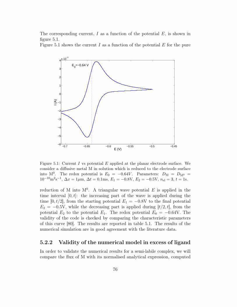
The corresponding current, I as a function of the potential E, is shown infigure 5.1.Figure 5.1 shows the current I as a function of the potential E for the pure

−0.7 −0.65 −0.6 −0.55 −0.5 −0.45−6

−5

−4

−3

−2

−1

0

1

2

3

4x 10

−3

E (V)

I (A

)

E0=−0.64 V

Figure 5.1: Current I vs potential E applied at the planar electrode surface. Weconsider a diffusive metal M in solution which is reduced to the electrode surfaceinto M0. The redox potential is E0 = −0.64V . Parameters: DM = DM0 =10−10m2s−1, ∆x = 1µm, ∆t = 0.1ms, E1 = −0.8V, E2 = −0.5V, nel = 3, t = 1s.

reduction of M into M0. A triangular wave potential E is applied in thetime interval [0, t]: the increasing part of the wave is applied during thetime [0, t/2], from the starting potential E1 = −0.8V to the final potentialE2 = −0.5V, while the decreasing part is applied during [t/2, t], from thepotential E2 to the potential E1. The redox potential E0 = −0.64V. Thevalidity of the code is checked by comparing the characteristic parametersof this curve [80]. The results are reported in table 5.1. The results of thenumerical simulation are in good agreement with the literature data.

5.2.2 Validity of the numerical model in excess of ligand

In order to validate the numerical results for a semi-labile complex, we willcompare the flux of M with its normalised analytical expression, computed

76

Observed values Theoretical valuesIa/Ic 1.2 1.0

Ep − Ep/2 (mV) 19.8 18.8Ec

p − Eap (mV) 21.9 19.7

Table 5.1: Comparison between the data observed from the simulation shown infigure 5.1 and the theoretical data computed given in [80] (Ia is the anodic current,Ic is the cathodic current, Ec

p is the peak potential, Ep/2 is the potential at halfpeak height; superscript a and c are for anodic and cathodic, respectively). Theresults shows good agreement with the data reported in literature.

by solving the problem in excess of ligand, in the Laplace domain [74]. Thenormalised flux is defined as the ratio between the current flux of M, JM, andthe flux of M in solution with the same total amount of M but no ligand,JM,noligand:

Φn(t) =JM

JM,no ligand

(5.2)

The analytical expression of equation (5.2), which has been computed in [74]for perfect sink conditions at a planar electrode surface:

Φ(t) =

√πDMt

c∗M,tot

L−1[(dcM

dt

)

x=0

]

(5.3)

where L−1 denotes the Laplace inverse transform. The inverse transformhas been numerically computed by applying the matlab-script INVLAP.Mavailable on the web [81]. The relative error of the normalised flux is definedas:

εr =|Φn − Φ|

Φn

(5.4)

Figure 5.2 shows the time evolution of the flux obtained with our model. Theexplicit expression for the analytical solution does not exist for the generalcase, but only for fully labile (solid curve in figure 5.2) or fully inert com-plexes (dashed-dotted curve in figure 5.2). The complete numerical method,shown in algorithm 3 at page 3, shows the general behaviour of a kineticallyintermediate complex, which passes from inert to a labile. At short times,δM is very small, and there is no time for the complex ML to dissociate inthe diffusion layer. Thus, the behaviour is that of an inert complex and thenumerical results fit the exact solution for inert complexes, equation (2.16):

Jin =DM[M]∗

δM

77

0 0.02 0.04 0.06 0.08 0.10

0.5

1

1.5

2

2.5

3

3.5

4x 10−7

t (s)

JM

(m

ol/m

2 s)

Figure 5.2: Flux at a planar electrode surface for an intermediate kinetic casecomputed with RD scheme: for short times the complex is inert (µML > δM),but at long times the complex is labile (µML < δM) due the increase of δM withtime. Solid line (-): equation (2.17), dashed-dotted line (-.): equation (2.16),crossed line (+): numerical results. Parameters:∆x = 1µm, ∆t = 0.25ms, DM =DML = DL = 10−9m2s−1, ka = 1000m3mol−1s−1, kd = 10s−1, K ′ = Kc∗L = 1,[M]∗ = 5 · 10−4molm−3, [ML]∗ = 5 · 10−4molm−3, [L]∗ = 1molm−3

At very long times, δM has increased very much and complexes have plentyof time to dissociate in the diffusion layer. They behave as fully labile com-plexes and the numerical curves tend towards the exact solution for the labilelimiting case, equation (2.17):

Jlab =DM[M]∗tot

δM

For intermediate times, both chemical kinetics and diffusion influence theflux.Our results compare well with well-known systems already investigated inthe literature. In particular, figure 5.3 shows the plot of the normalisedflux, equation (5.2), at the surface, computed respectively by applying i)the complete scheme, equation (3.23) (dash-dotted line, indicated as NS inthe figure), ii) the RD scheme, equations (4.4)-(4.6) (dashed line) and iii)the equation (5.3) (circles). The graph covers fluxes for inert (short times),

78

10−2

100

1020.05

0.1

0.15

0.2

0.25

0.3

0.35

0.4

t (s)

ΦRD

NS

Figure 5.3: Comparison of the flux computed by numerical inversion of the analyt-ical flux solution, equation (5.3) (circles) and by numerical simulation obtained bycomplete scheme (3.23) (dashed-dotted line) and RD scheme (dashed line) for 100seconds of electrolysis. ∆x = 50µm, ∆t = 0.1ms, DM = 10−7m2s−1, DL = DML =10−11m2s−1, ka = 10m3mol−1s−1, K = 10m3mol−1, [L]∗ = 1molm−3. The circlevalues (o) are taken from table 2 (column a) of [74].

labile (long times) and kinetically intermediate cases. The values obtainedwith our numerical procedure are in perfect agreement with the literaturedata [74] obtained by the analytical solution (circles).An important result must be emphasised: the excess of ligand case can al-ways be solved numerically with the complete scheme (3.23), i.e. withouttime splitting, if the condition ∆t < 2

ka[L]∗is fulfilled (see the discussion sec-

tion 3.4 at page 32). The advantage of the splitting procedure, however, isthat the excess of ligand case can be solved for any value of the associationand dissociation rate constants, ka and kd, and of the diffusion coefficientsDM and DML and in principle with quite large integration time ∆t by applyingimplicit methods [23]. (Notice that, the condition ∆t < 2

ka[L]∗is sufficient,

because we usually work with K[L] ≥ 1 which implies k−1a [L]−1 < k−1

d . There-fore ∆t < k−1

a [L]−1 < k−1d ).

This result opens up the possibility to choose the most suitable numericalmethod to solve the reaction process with either an explicit or an implicitmethod. In particular, we can apply an implicit Euler method, equation (4.7),

79

which works for any value of the association-dissociation rate constants.However, it is not the goal of this thesis to investigated the advantages inusing an implicit method. Thus, in the rest of the thesis, we will always usethe explicit method.Figure 5.10, at page 87, shows the concentration profiles of a semilabilecomplex ML at different times, computed by applying the complete schemewith the grid refinement scheme, by using two subgrids. At very short time(t = 0.01 s), it behaves as a non labile complex, while at longer times (t > 0.15s) it behaves as close to labile. Figure 5.10 c) shows the error on the flux com-putation, compared with the analytical equation 5.3, computed with equation(5.4). The important point is that, the error is acceptable at any time, i.e.for any degree of lability of the complex. Thus, it shows that the grid re-finement can be satisfactorily applied for semilabile case irrespective of thecontribution of the complex ML.

5.3 Some studies with simple multiligand sys-

tems

5.3.1 Mixture of ligands in excess compare to metal

The above results can be extended to the case of a mixture of ligands. Indeed,in case of nl ligands, jL, present in the solution, with j running from 1, . . . , nl,we have to deal with nl parallel reactions (2.19), which introduce in theprocess nl reaction times of the order of (jka[

jL])−1. Therefore, as shown insection 3.4, to get convergence under the excess of ligands case, the spectralradius of the iteration matrix is less than one only if

∆t < minj

2(jka[jL])−1 (5.5)

which means that the fastest reaction determines the time integration stepto use.

Figure 5.4 shows an example of flux computation by applying the RDscheme to two ligands 1L and 2L which can react with M. In figure 5.4 thereaction involving 1L is much faster than that involving 2L. Unfortunatelythere is no analytical solution for this case, as far as we know. So no com-parison with theoretical curve is possible. However, the plot of this flux, infigure 5.4, is fully reasonable, in particular when it is compared to the fluxescomputed by equations for the fully inert (equation (2.16) page 17) and fullylabile complexes (equation (2.17) page 17), respectively. Indeed, considering

80

0 0.1 0.2 0.3 0.4 0.50

1

2

3

4

5x 10−8

t (s)

JM

(m

ol/m

2 s)

Figure 5.4: Two complexes, ML1 and ML2 with ligand excess. Parameters: DX =

10−10m2s−1 for all the species, k(1)a = 104mol−1m3s−1, k

(1)d = 103s−1, k

(2)a =

10−2mol−1m3s−1, k(2)d = 10−3s−1, [M]∗tot = 10−3molm3, [1L]∗ = [2L]∗ = 1molm3,

[M1L]∗ = [M2L]∗ = 4.76 · 10−4molm3, ∆t = 10−5s, ∆x = 0.05µm, nx = 1000. Theplot shows the flux computed by applying the RD scheme. It is compared with thefluxes under the fully inert (green solid line -) and labile (red dashed-dotted line -.)conditions, equation (2.16) and (2.17) respectively, with DM defined in equation(2.18).

81

the kinetics of the two complexes, we can expect M2L to be inert even atthe largest tested time, whereas M1L will be labile at that time. So at longtimes, we expect a flux equal to about a half of that we would obtain fortwo fully labile complexes. Indeed, at t = 0.5s the flux, assuming two fullylabile complexes, is equal to 8 · 10−9mol m−2s−1, while the computed flux is4.1 · 10−9mol m−2s−1.Figure 5.5 shows the concentration profiles near the electrode, for the same

Figure 5.5: Profiles in a system with two complexes, M1L and M2L with ligandexcess. Concentration profiles of M and M1L as a function of the distance x fromthe electrode surface. The concentration ratio depicted in the inset is defined as[X]/[X]∗ for X=M and M1L. Other parameters are as in figure 5.4. The reactionlayer thickness for the reaction M+1L­M1L is µM1L = 0.1µm. The profile con-centrations of 1L, 2L and M2L are not shown because they are horizontal due tothe excess of 1L and 2L and the very low dynamics of M2L.

example as above. The so-called normalised concentration (inset) of a speciesX is given by the ratio [X]/[X]∗ where X∗ is the bulk concentration. We cansee that the complex M1L is almost completely depleted close to the electrodesurface (as expected for a labile complex), while M2L is not depleted at all(inert complex). The thickness of the reaction layer, µM1L, can be estimatedfrom the inset of figure 5.5, at the crossing of the two tangents of the curveof M. A value of ∼ 0.1µm is obtained, which corresponds to the theoreticalvalue of 0.1µm, equation (2.12). This is another validation of the numerical

82

scheme.Notice that the normalised concentration profile of M1L collapses with thatof M for x > µM1L, which is expected under conditions where M and M1Lare at equilibrium.

5.3.2 Computation of flux without ligand excess

We studied the capability of the method for a process involving two ligands,1L and 2L which are not in excess compared to M. As in the example shown infigure 5.4, we consider two reactions with very different time scales. The fluxcomputed by applying the RD scheme is shown in figure 5.6. The reaction

0 0.2 0.4 0.6 0.8 10

0.5

1

1.5

2x 10−8 flux

t (s)

JM

(m

ol/m

2 s)

Figure 5.6: Two complexes, M1L and M2L, without ligand excess. Parame-ters: D = 10−10m2s−1 for all the species, 1ka = 106mol−1m3s−1, 1kd = 102s−1,2ka = 10−2mol−1m3s−1, 2kd = 10−6s−1, [M]∗tot = 10−3molm−3, [1L]∗ =[2L]∗ =5·10−4molm−3, [M1L]∗ =[M2L]∗ = 4.55·10−4molm−3, [M]∗ = 9×10−5, ∆t = 10−3s,∆x = 0.3µm, nx = 300. The plot shows the flux computed with the RD schemecompared with the flux of the fully inert (green solid line –) and fully labile (reddashed-dotted line -.) complexes in excess of ligands, equations (2.16) and (2.17)respectively.

involving 1L is much faster than that involving 2L, and thus (given the ac-tual concentrations and diffusion coefficients) the major contribution to theflux JM is expected to originated from the complex M1L. This is confirmedin figure 5.7 where the normalised concentration profiles of the species areplotted as a function of the distance from the electrode surface.Interestingly, in absence of ligand excess, the normalised concentration curves

83

0 5 10 15 200

0.2

0.4

0.6

0.8

1

x (µ m)

ratio

of c

once

ntra

tions

L1

ML1

M

Figure 5.7: Two complexes, M1L and M2L, without ligand excess. Normalisedconcentration profiles of M, M1L and 1L, as a function of the distance from theelectrode. Other parameters as in figure 5.6. The reaction layer thickness for thereaction M+1L­M1L is µM1L = 0.45µm. The normalised concentration profiles of2L and M2L are not shown because they are horizontal and equal to 1.0, due tothe very low dynamics of M2L.

of M and M1L merges at distance very far from the reaction layer, showingthat equilibrium is not reached at any point of the diffusion layer. Althoughno comparison of the numerical computation could be done with an analyt-ical solution, the code was validated in two ways: i) at long times, JM isabout half of the flux which would be obtained for fully labile complexes (asin figure 5.4) and ii) the sum of [1L] and [M1L] at any distance x, is alwaysequal to [1L]∗tot within experimental errors. In addition, the observed valueof µM1L is ∼ 0.40µm coincides with that computed theoretically ∼ 0.45µm.

5.3.3 Mixture of complexes; the use of several grids

Figure 5.8 shows an example of 2 reactions with an excess of ligand ([M]tot =0.012 mol m−3, [1L]∗tot = 1.01 mol m−3 and [2L]∗tot = 1.001 mol m−3). Fol-lowing the procedure outlined at page 67, we use three grids, such that thefirst interface, denoted with Γ1,2, is placed at x = 2µM1L and the second one,denoted with Γ2,3, is placed at x = 2µM2L. In this example, the first complexM1L, which is the fastest one, contributes to the flux much more than thesecond complex M2L. The reaction layer thicknesses are µM1L = 1µm andµM2L = 10µm respectively. The value of the subgrid size ∆x1 is chosen to

84

10−7

10−6

10−5

10−40

0.2

0.4

0.6

0.8

1

x (m)

[X]/[

X]*

M1L

M2L

2L

1L

M µ1

µ2

Γ1,2

Γ2,3

Figure 5.8: Plot of the normalised concentration profiles of the species at t = 1s,by using the grid refinement scheme. Parameters are: for all species diffusioncoefficients equal to 10−10m2s−1, 1ka = 100 m3 mol−1 s−1, 2ka = 1 m3 mol−1

s−1, 1kd = 10 s−1, 2kd = 1 s−1, ∆x1 = µ1/10, ∆t = 10−3s, nx = 282, [M]∗ =10−3 mol m−3, [1L]∗ = 1mol m−3, [2L]∗ = 1 mol m−3, [M1L]∗ = 10−2 mol m−3,[M2L]∗ = 10−3 mol m−3. The interfaces between subgrids Γ1,2 and Γ2,3 are shownwith continuous lines. Γ1,2 and Γ2,3 are respectively placed at 2µ1 and 2µ2 fromthe electrode surface. (Notice that in this plot we have assumed µ1 = µM1L andµ2 = µM2L).

be less than µM1L and µM2L: ∆x1 = µM1L/3. Furthermore, the time stephas been fixed to ∆t = 1ms, so that it is short enough to get convergenceand large enough to get reasonable computation time. Indeed, by applyingthe convergence criteria in appendix B, the time convergence condition is∆t < 102s. This example also shows that the grid refinement technique canbe applied for complex systems involving more than one reaction.Figure 5.3.3 shows the concentration profiles of the species for two parallelreactions involving two ligands 1L and 2L which can react with M to form twoseparate complexes M1L and M2L. We have chosen 3 subgrids. The reactionshave the same equilibrium constants 1K = 2K = 100 mol m−3 but differentassociation-dissociation rate constants. There is a slight excess of ligand 1Land no excess of ligand 2L. Bulk concentrations are: [M]∗tot = 3.1 mmol m−3,[1L]∗tot = 1.1 mmol m−3 and [2L]∗tot = 4 mmol m−3. These ligands are not in

85

10−6

10−50

0.2

0.4

0.6

0.8

1

x (m)

[X]/[

X]*

M

M2L

M1L

1L

2L

µ1µ

2

Γ1,2 Γ

2,3

Figure 5.9: Plot of the normalised concentration profiles of the species at t = 0.5s,by using the grid refinement scheme. Parameters are: all diffusion coefficients equalto 10−10m2s−1, 1ka = 100 m3 mol−1 s−1, 2ka = 200 m3 mol−1 s−1, 1kd = 1 s−1,2kd = 2 s−1, [M]∗tot = 3.1 mmol m−3, c1L,tot = 1.1mmol m−3, c2L,tot = 4mmol m−3,∆x1 = 4.18 · 10−7m, ∆t = 10−4s, nx = 59, [M]∗ = 10−3 mol m−3, [1L]∗ = 10−3

mol m−3, [2L]∗ = 2 · 10−3 mol m−3, [M1L]∗ = 10−4 mol m−3, [M2L]∗ = 2 · 10−3

mol m−3. (Notice that in this plot we have assumed µ1 = µM1L and µ2 = µM2L).

excess, in fact figure shows that there is a slight increase of [1L] and [2L] nearthe consuming surface. So, according to equation (2.12) the reaction layerthicknesses vary with time. However, by considering that the dynamics ofthe system is not very high (1ka[1L]∗ = 0.1s−1, 2ka [2L]∗ = 0.4s−1, 1kd = 1s−1

and 2kd = 2s−1), we can use the bulk values of free ligands to estimate thereaction layer thicknesses. Such approximated values are: µM1L ∼ 30µm andµM2L ∼ 16µm. The value of the finest grid, ∆x1 = 0.418µm, has been chosento be less than both reaction layers (approximately 30 and 70 times smaller)and therefore we might expect a good numerical precision. Also, ∆t is withinthe domain of convergence of the numerical scheme. The results show goodvalues. As the rate constants of the complexation process with 2L are largerthan with 1L, the concentration profile of M2L is more depleted and resem-bles to that of M more than the profile for M1L (i.e. M2L is more labile thanM1L).

86

a) b)

10−8

10−60

0.2

0.4

0.6

0.8

1

x (m)

[X]/[

X]*

M

ML

L

µ1 δx

s 10−50

0.5

1

x (m)

[X]/[

X]*

M

ML

L

µ1

xs

δ

c)

0 0.02 0.04 0.06 0.08 0.10

1

2

3

4

5

t (s)

ε r (%

)

Figure 5.10: Example of the application of the grid refinement method for a semi-labile complex ML. Figure a) and b) show the concentration profiles of the speciesat t = 0.01s and t = 0.1s respectively corresponding to different degrees of lability.Figure c) shows the error given by equation 5.4, ranging from non labile to labilecase. Parameters are: [M]∗tot = 10−3 mol m−3, [L]∗tot = 1 mol m−3, ka = 104

m3 mol−1 s−1, kd = 500 s−1, DM = DL = DML = 10−10 m2 s−1, xs = 2µML,∆x1 = µML/50, µML = 10−7m, ∆x2 = 2µML, ∆t = 0.01ms (xs denotes the inter-face of separation between the subgrids.)

87

Chapter 6

Fluxes in environmentalMultiligand systems

6.1 Overview

In this chapter we consider environmental multiligand systems. The attentionis focused on the computation of the so-called maximum flux. It is obtainedwhen the interfacial process is so fast that the limiting factors to the fluxare diffusion and chemical reactions in solution only. This maximum flux isthus independent of the nature of sensor or microorganism. It only dependson the physical and chemical composition of the environmental medium,and it is thus a key factor to characterise the environment with respect tobioavailability of metals and consequently ecotoxicology.This chapter is organised as follows. Section 6.2 gives a brief summary of thephysical problem with the governing equations and the corresponding initialand boundary conditions. Section 6.3 gives the metal flux computations inpresence of the two simple inorganic ligands, which are the most important inaquatic systems: carbonate CO2−

3 and hydroxyl OH−. Section 6.4 discussesthe role of Fulvic substances on the metal flux, while section 6.5 studies themetal flux in presence of suspended particles/aggregates. Finally, section 6.6studies the metal flux of two typical aquatic systems, containing a mixtureof the above environmental complexants.

89

6.2 A summary of the physical model and bound-

ary and initial conditions

We consider the mathematical formulation of metal flux at a planar consum-ing surface in multiligand systems given in chapter 2, precisely the problemstated by equations (2.24) - (2.27).In all cases, the initial conditions are the following:

• the bulk solution is homogeneous

• all species are in equilibrium in the bulk solution, and

• the bulk concentrations of any species is independent of time.

The boundary conditions related to each species at the consuming interfaceare the following:

• M is consumed at the interface and its concentration [M]0 on the solu-tion side of the surface (subscript 0) is nil. This condition correspondsto very fast transfer rate of M through the interface, i.e. to maximumflux, in the solution phase.

• MjLi does not pass through the interface, equation (2.32).

• A complex can only be consumed after dissociation into M and jL

• jL does not pass through the interface, equation (2.33).

• The flux is computed under conditions of finite planar diffusion, i.e. theconcentrations of all species are assumed to be equal to those in the bulksolution, at a finite distance (around 20µm) of the consuming interface.This corresponds to conditions valid in stirred solution, equation (2.30).

The set of equations (2.24) - (2.27) with the initial (bulk) and boundaryconditions stated above for each species, describes a typical complex reaction-diffusion system. This system is solved by applying the algorithm 3 definedat page 68, from which we have developed a fortran 90 numerical code, calledMHEDYN (available on the internet, see the introduction at page 6). Theuser can decide the time step of integration of diffusion and reaction andthe first grid size ∆x1 (the closest to the consuming surface). Here we havedecided to fix the same time step, ∆t = 0.5∆tmin, where ∆tmin is computedby MHEDYN by applying the convergence criteria stated in appendix B.The subgrids and their size and position are automatically determined bythe procedure outlined in section 4.3.4 at page 67. On the other hand, if

90

MHEDYN is not able to automatically set the subgrids, because there couldbe many ligands or the reaction layer thicknesses might be too close to eachother. So the user must decide the subgrid parameters by imposing the valuesof the first subgrid size ∆x1, its number of discretization points n1 and thegrid refinement factor g.All the results shown in this chapter have been computed by using this code.Unless otherwise stated, the results of the simulations are at steady-state.The total flux of metal through the interface is given by

Jtot =1

A

(dN

dt

)

x=0(6.1)

where A is the surface area of the interface and N the number of moleof metal ion. The contribution of each individual complex to the flux canbe expressed in terms of its degree of lability jξi. For the global systemthe lability degree is defined [13] as the ratio of the flux provided by thecomplexes over the same contribution if all the complexes were fully labile(i.e. able to dissociate completely at the interface). In the case of ligandexcess under steady-state conditions, the particular degree of lability jξi hasbeen shown (see appendix C) to be computed with the following equation:

jξi =1 − [MjLi]

0

[MjLi]∗

1 − [M]0

[M]∗

(6.2)

where [MjLi]0 is the surface concentration of MjLi, provided at any time by

the numerical simulation.The derivation of the lability degree given in appendix C is new because,for the first time, mixtures of ligands and their successive metal complexeshave been considered together. In particular, the derivation of equation (6.2)follows the same line of reasoning made in [13, 82] for simple complexes andsuccessive complexations, separately.Under steady-state conditions, the individual flux of MjLi is related to thedegree of lability by (see appendix C):

JMjLi=

DMjLi[MjLi]

∗

δ

(

1 − [M]0

[M]∗

)

jξi (6.3)

The values of the association rate constants, for complexes with simple lig-ands and fulvics/humics, are computed as discussed in [83]. They are givenby:

kMLa =

kOSa k−w

kOSd + k−w

(6.4)

91

where k−w is the rate constant for elimination of a water molecule from theinner shell of the free hydrated metal ion. The expressions for kOS

a and kOSd

are the following:

kOSa =

4πNava(DM + DL)U(a)kBT

eU(a)kBT − 1

(6.5)

kOSd =

3(DM + DL)U(a)kBT

a2(eU(a)kBT − 1)

eU(a)kBT (6.6)

where Nav is the Avogadro number, kB is the Boltzmann constant, T is thetemperature (T = 273K), a is the distance of closest approach of the metaland the ligand (a = 0.5nm), DM and DL are the diffusion coefficients of themetal M and the ligand L respectively and U(a) is the electrostatic interactionenergy of M and the complexing site L, at their distance of closest approacha.If U(a)= 0 then the above equations simplify in:

kOSa = 4πNava(DM + DL) (6.7)

kOSd =

3(DM + DL)

a2(6.8)

For simple ligands [84]:

U(a) =zMzLe2

4πε0εa

(

1 − κa

1 + κa

)

(6.9)

where

κ =

√

2Nave2I

ε0εkBT(6.10)

and ε is the relative dielectric constant of water, ε0 is the vacuum permittivityand e is the electric charge.For Humic substances [83]:

U(a) = zMeψ (6.11)

where ψ is the electric potential at the surface of the humics, due to theirnegative charge. Its values is discussed in [85].Environmental "particles" are usually aggregates with wide size distribution.It has been shown that [83], as a first approximation, the effective associationrate constants of their metal complexes, can be computed by [17, 86]:

ka =kML

a

1 + B(6.12)

92

where

B =kML

a |L|tot ∆Sb

Sb,tot

4πrDMcp

(6.13)

where |L|tot is the total concentration of complexing sites, ∆Sb

Sb,totis the fraction

of surface area, for particle with radius r and cp is the number concentrationof particle aggregates. The potential U(a) is also given by equation 6.11,where ψ is the surface potential at the site L (see [83] for values).

6.3 Metal fluxes in presence of simple Ligands:

OH− and CO2−3

6.3.1 Metal complex distribution and simulation condi-tions

Preliminary tests have shown that, amongst the simple inorganic ligands andunder natural conditions, OH− and CO2−

3 are the most important ones tostudy. Other complexes are either not stable enough to play a significantrole, or fully labile so that they do not influence significantly the total flux.Two series of simulations have been performed in presence of total Cu2+

concentration, [Cu]tot = 10−8M:

1. At constant total carbonate concentration, [CO2−3 ]tot = 2× 10−3M and

pH varying between 4 and 9

2. At constant pH’s = 7, 8 and 9 with [CO2−3 ]tot values varying between

10−5M and 10−1M.

Only complexes Cu(OH)+, Cu(OH)02, CuCO0

3 and Cu(CO3)2−2 are present in

significant proportions under those conditions. The corresponding distribu-tion of metal species in the bulk solution, were computed by MINTEQ [87]and are given in figures 6.1, 6.2 and 6.3.

Metal flux under different conditions of pH and [CO2−3 ]tot are shown from

figures 6.4 to 6.12. Whenever possible, additional tests of the validity of thenumerical procedure developed here, are shown by comparing the results ofMHEDYN with those of another code, FLUXY (see [17] for a complete de-scription of this code). This latter code performs calculations at steady-stateand in excess of ligand only. The fluxes and the lability degrees, obtainedwith this code, are refereed to in the figures with the name "FLUXY". Thevalues of stability constants and dynamic constants (diffusion coefficients andchemical rate constants) used to obtain these figures are given in tables D.1

93

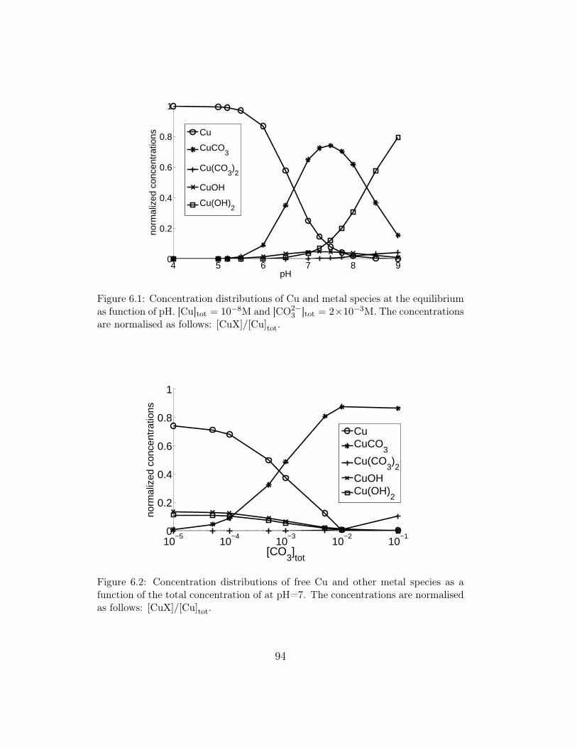
4 5 6 7 8 90

0.2

0.4

0.6

0.8

1

pH

norm

aliz

ed c

once

ntra

tions Cu

CuCO3

Cu(CO3)2

CuOH

Cu(OH)2

Figure 6.1: Concentration distributions of Cu and metal species at the equilibriumas function of pH. [Cu]tot = 10−8M and [CO2−

3 ]tot = 2×10−3M. The concentrationsare normalised as follows: [CuX]/[Cu]tot.

10−5

10−4

10−3

10−2

10−10

0.2

0.4

0.6

0.8

1

[CO3]tot

norm

aliz

ed c

once

ntra

tions

CuCuCO

3Cu(CO

3)2

CuOHCu(OH)

2

Figure 6.2: Concentration distributions of free Cu and other metal species as afunction of the total concentration of at pH=7. The concentrations are normalisedas follows: [CuX]/[Cu]tot.

94

10−5

10−4

10−3

10−2

10−10

0.2

0.4

0.6

0.8

1

[CO3]tot

[CuX

]/[C

u]to

t

CuCuCO

3

Cu(CO3)2

CuOHCu(OH)

2

Figure 6.3: Concentration distributions of Cu and other metal species as a functionof the total concentration of CO2−

3 at pH=9. The concentrations are normalisedas follows: [CuX]/[Cu]tot.

to D.11 of appendix D. The diffusion coefficients of complexes are assumedto be equal to those of Cu2+. The values of association rate constants jka,i

of a complex MjLi are computed as discussed in [83] and briefly summarised

in section 6.2. The values of jkd,i are obtained from jkd,i =jka,ijKi

6.3.2 Results at constant [CO2−3 ]tot and varying pH

Figures 6.4 and 6.5 show the change of total normalised flux and the degree oflability, jξi, of individual species, as function of pH, for [CO2−

3 ]tot = 2×10−3M.In figure 6.4, the total flux, JM, is normalised with respect to the totalflux, Jlab, which would be obtained if all complexes were fully labile (i.e. ifthey were fully consumed after dissociation at the interface, equation (2.17)).Figure 6.4 also shows for comparison the fraction of Cu2+ in the bulk solution,with respect to the total concentration of Cu. If all complexes were fullylabile at any pH, JM/Jlab would be a horizontal line. If all complexes werefully inert, the curve of JM/Jlab would coincide with that of [Cu2+]

[Cu]tot. Clearly,

figure 6.4 shows that the behaviour of the system is in between these twolimits, indicating that some of the complexes are semi-labile at pH≥7. Figure6.5 which provides the degree of lability of each metal complex, shows thatthe lability of all of them decreases above pH=7. Figure 6.6 provides the

95

4 5 6 7 8 90.0

0.2

0.4

0.6

0.8

1.0

[Cu2+

]/[C

u]to

t

J tot/J

lab

pH

Figure 6.4: The plot shows the computed flux (normalised with the labile flux)and the corresponding free Cu concentration (continuous line) , as a function ofpH. Other parameters: [CO2−

3 ]tot = 2× 10−3M, [Cu]tot = 10−8M. The thickness ofthe diffusion layer is ∼ 20µm. Other parameters from tables D.1 to D.6 at page180–185.

4 5 6 7 8 90

0.2

0.4

0.6

0.8

1

pH

j ξ i

CuOH

Cu(OH)2

CuCO3

Cu(CO3)2

Figure 6.5: Lability degree, computed with equation (6.2), of the four metal speciesas function of pH in the same conditions of figure 6.1

96

4 5 6 7 8 90

20

40

60

80

pH

j Ji/ J

tot (

%)

CuOH

Cu(OH)2

CuCO3

Cu(CO3)2

Figure 6.6: Proportion of individual fluxes jJ , computed with equation (6.3), ofeach complex in total flux. Same conditions as in figure 6.1.

proportion of the individual contribution, jJ , of each metal species, to thetotal flux J given in figure 6.4. It shows that at pH=7, CuCO3 provides themain contribution to the total flux. This is expected, since this complex isin dominant proportion and fully labile at that pH. At pH’s larger than 8,Cu(OH2) becomes the largest contributor to the flux.

6.3.3 Results at constant pH and variable [CO2−3 ]tot

Figures 6.7, 6.8, and 6.9 show the changes of the normalised total flux,JM/Jlab at pH=7, 8 and 9, respectively. These figures also show the re-sults obtained with FLUXY. They are in good agreement with the fluxescomputed by MHEDYN. Figure 6.7 shows that, at pH=7, all the species arelabile for most of the tested [CO2−

3 ]tot concentration values. On the otherhand, as the pH increases the total flux decreases (figure 6.8, and 6.9). Thetotal flux takes maximum values when [CO2−

3 ]tot ∼ 10−3 − 10−2M.To understand the reason of the maximum, figure 6.10 shows the degree oflability of each complex, jξi, as a function of [CO2−

3 ]tot, at pH=9. All com-plexes are semilabile and their degree of lability show a maximum value inthe same range of total carbonato concentrations as mentioned above. Fig-ures 6.11 and 6.12 show the effective contributions of each species to the totalflux. Comparing these two figures, we can say that at i) pH=7, the majorcontribution to the flux is given by free Cu when [CO2−

3 ]tot < 10−3M and byCuCO3 when [CO2−

3 ]tot > 10−3M and ii) at pH=9, the major contribution

97

-5 -4 -3 -2 -10.0

0.2

0.4

0.6

0.8

1.0

[Cu2+

]/[C

u]to

t

J tot/J

lab

log([CO3]

tot/M)

Figure 6.7: Total flux normalised with the labile flux as function of [CO2−3 ]tot at

pH=7. [Cu]tot = 10−8M. The normalised concentration of free Cu2+ is given forcomparison. Other parameters from table D.7 to table D.10, at page 186–189.

to the flux is given by Cu(OH)2 when [CO2−3 ]tot < 10−2M and by Cu(CO3)2

when [CO2−3 ]tot > 10−2M and iii) the contribution of free Cu is negligible

at pH=9. Thus, the whole of the results of figure 6.7 to 6.12, suggeststhat the maximum fluxes observed in figures 6.8 and 6.9, are more due toan intrinsic change of lability of all these complexes, as function of pH or[CO2−

3 ], rather than to the change of their thermodynamic distribution asfunction of pH or [CO2−

3 ].

6.4 Metal fluxes in presence of Fulvic Acids

6.4.1 Simulation conditions

Humic and fulvic substances include a whole of analogous but not identicalmolecules, and, as a whole, behave as chemically heterogeneous polyelec-trolytic complexants with rather small size distribution [88]. Due to chem-ical heterogeneity, M forms with fulvics a very large number of differentcomplexes, MjL. In order to better understand the role of these complexesin environmental systems, in particular on metal biouptake, the major goalsof the simulations below are i) to determine the time evolution required toreach the maximum flux at steady state, due to Cu2+-fulvic complexes andto compare it with the corresponding flux, Jlab, which would be observed if

98

-5 -4 -3 -2 -10.0

0.2

0.4

0.6

0.8

1.0

J tot/J

lab

log([CO3]

tot/M)

Figure 6.8: Total flux normalised with the labile flux as function of [CO2−3 ]tot at

pH=8. Same conditions as in figure 6.7.

-5 -4 -3 -2 -10.0

0.2

0.4

0.6

0.8

1.0

J tot/J

lab

log([CO3]

tot/M)

Figure 6.9: Total flux normalised with the labile flux as function of [CO2−3 ]tot at

pH=9. Same conditions as in figure 6.7.

99

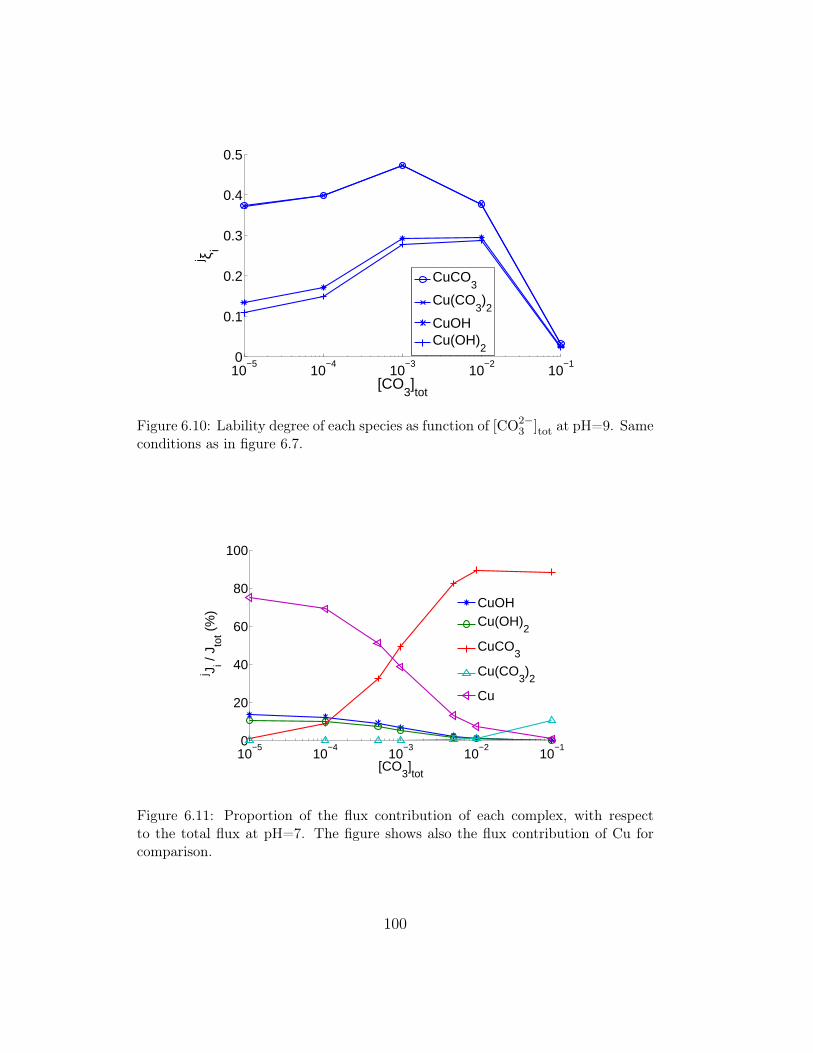
10−5

10−4

10−3

10−2

10−10

0.1

0.2

0.3

0.4

0.5

[CO3]tot

j ξ i

CuCO3

Cu(CO3)2

CuOHCu(OH)

2

Figure 6.10: Lability degree of each species as function of [CO2−3 ]tot at pH=9. Same

conditions as in figure 6.7.

10−5

10−4

10−3

10−2

10−10

20

40

60

80

100

[CO3]tot

j J i / J to

t (%

)

CuOHCu(OH)

2

CuCO3

Cu(CO3)2

Cu

Figure 6.11: Proportion of the flux contribution of each complex, with respectto the total flux at pH=7. The figure shows also the flux contribution of Cu forcomparison.

100

10−5

10−4

10−3

10−2

10−10

20

40

60

80

100

[CO3]tot

Jto

t/ Jla

b

CuCuCO

3

Cu(CO3)2

CuOHCu(OH)

2

Figure 6.12: Proportion of the flux contribution of each complex, with respectto the total flux at pH=9. The figure shows also the flux contribution of Cu forcomparison.

all complexes were labile, and ii) to determine the type of fulvic sites whichprovide the complexes with the largest contribution to the total flux.It is out the scope of this thesis to describe the kinetic and thermodynamicproperties of the metal fulvic complexes [83, 89, 90, 1, 88, 85]. The pa-rameters used in the present simulations have been obtained as described insection 6.2 and in more detail in [83]. Briefly thermodynamic properties ofmetal-fulvic complexes are represented by Freundlich isotherms and linearSips distribution, based on the assumption that metal forms 1:1 complexes,with an infinite number of different site types. This distribution correspondsto an increase of the molar fraction of strong binding site (with respect tothe whole of fulvic sites) with a decrease of their complexation strength [90].The site types of fulvics can be classified in minor and major ones [90], byreferring to their proportions. The minor ones are the strongest and the mostimportant for trace metal binding under natural conditions. It has been es-timated that each fulvic molecule includes not more than one such minorsite [83]. In addition when minor sites are dominant, i.e. at low metal/fulvicconcentration ratio, the relationship between the cumulative molar ratio ofa site j, jχ, and its stability constant jK, is given by [89, 90, 83]:

logiχ = −0.174 − logσ + ΓlogK∗0 − ΓlogiK (6.14)

where σ is the total density of sites (in mol/g) in the fulvics and Γ and K∗0 are

characteristic constants of the metal and the fulvics at the given pH, ionic

101

strength and temperature. Γ represents the chemical heterogeneity of thefulvics. It is always comprised between 0 and 1 and is often close to 0.5. Theoverall complexation properties of the fulvic molecules can be represented bythe following relationship:

K∗ =[ML]

[M][L](6.15)

where [ML] is the total concentration of complexes with all sites, [L] is thetotal concentration of free sites, and K∗ is the so called differential equilib-rium function [89, 91, 90]. K∗ is, in fact, an average of all jK, weighted bytheir molar fraction and their degree of occupation. Thus K∗ is a functionwhich depends on the pH, ionic strength and metal ligand ratio. It can beshown that for Γ = 0.5, under a set of conditions, K∗ is equal to the value ofjK whose sites are half saturated by M [90]. K∗ is a useful parameter sinceit can be easily computed from experimental data through:

log[M]totFS = ΓlogK∗

0 − logK∗ (6.16)

Figure 6.13 shows the distribution of the concentrations of complexes CujLas function of LogjK, for Γ = 0.52, pH = 8 (logK∗

0 = 8.54), [Cu]tot = 10−6Mand a concentration of fulvics expressed as 5 mg C/l (C=Carbon). Thevalue of LogK∗(= 9.4 for these conditions) is also shown on the graph. ForlogjK ÀlogK∗ (e.g. logjK >logK∗ + 2), the sites are fully saturated, but insmaller and smaller number when jK increases. Thus the corresponding con-centration values of CujL tend to zero when jK → ∞. For logjK ¿logK∗

(e.g. logjK ¿logK ∗ −2), the complexation strength is weaker and weakerwhen jK decreases, and even though the site concentration increases, the con-centration of CujL also tends to zero at very low jK values. The dynamicparameters of fulvic and their complexes are given in tables E.1 to E.12 inappendix E for the four conditions discussed here. They are obtained asfollows [83]. The diffusion coefficients of all complexes CujL are assumedto be equal to those of the fulvics themselves (DFS = 2.8 × 10−10m2s−1 atpH = 8), which is a reasonable approximation considering that the size offulvics is much larger than that of free dehydrated M. The overall formationrate constants of CujL complexes, jka, are computed from the rate constantof elimination of water from the inner hydration shell of the metal ion andthose of formation and dissociation of the corresponding outer-sphere com-plex. In this latter case, the significant electrical potential inside the fulvicsmust be considered. The dissociation rate constants, jkd, are obtained fromjkd = jka/

jK.Based on the above considerations, at low metal/fulvic ratios (which are the

102

6 7 8 9 10 11 12 130

2

4

6

8x 10−8

Log K

[Cuj L]

(m

ol/L

)

Log K*

unsaturated sites saturated sites

Figure 6.13: Concentration distributions of Cu-Fulvic complexes in the bulk solu-tion for logK values ranging from 6.3 and 12.3. The vertical dashed lines representthe values of LogK∗ = 9.4, LogK∗ + 2 and LogK∗ − 2. They indicate the regionsof saturation, partial saturation and unsaturation of sites.

important conditions for vital and toxic metals) one can see the metal fulvicsolution as a mixture of complexes with widely different jK and jkd val-ues (different labilities), but the same diffusion coefficients (same mobilities).The overall flux will be the sum of all individual fluxes, each one dependingmainly on the concentration and degree of lability jξ of the correspondingcomplex. Thus in the following, interpretation of data will be based on dis-tribution curves of i) individual fluxes, jJ , and ii) degree of lability jξ withrespect to the stability constants of the corresponding sites, jK. On this lastaxis, the value of logK∗ is given, as well as the regions of full saturation,partial saturation and unsaturation of sites as defined above (figure 6.13).Because the distributions of lability degrees and complex concentrations asfunction of jK, depend significantly on pH and metal to fulvic concentrationratios, simulation have been run at two different pH’s (6 and 8) and [Cu]tot(10−8M and 10−6M) at constant FS = 5 mg C/L. In each case, the con-tinuous distribution of sites, expression (6.14), was discretized as discussedin [89, 83] by using 36, 31, 31 and 29 site types respectively, with logjKvalues separated by a constant interval of ∆logjK = 0.2. The overall testedrange of logjK was centred on logK∗, with minimum and maximum valuesof logjK located at logjKmin ≤logK∗ − 2 and logjKmax ≥logK∗ + 2 [83],their exact values being chosen to span the largest possible range of jK. Thecontribution of sites external to this range is indeed negligible.

103

Note that, for all sites with LogjK ≥LogK∗ − 1, cjL is not in excess withrespect to cMjL. However, MHEDYN has the capabilities to perform compu-tations under these conditions.

6.4.2 Time evolution of total flux and concentrationprofiles

Figure 6.14 gives the time evolution of the total flux, normalised with the to-tal flux at steady-state of equivalent but labile complexes, Jlab, under four pHand [Cu]tot conditions. It is seen that in all conditions, the steady-state is at-tained within one second or less, which suggests that under most environmen-tal conditions, only steady state fluxes must be considered, since most envi-ronmental processes occurs at time scales larger than one second. Figure 6.14also shows that, at steady-state and pH=6 and [Cu]tot = 10−6M, the wholeof the fulvic complexes behaves as almost fully labile complexes. However, athigher pH and lower metal/fulvic complexes (pH=8, [Cu]tot/FS = 2×10−3

mol/Kg) the whole of complexes behaves as non labile complexes. This resultis supported by a wealth of experimental data on metal-fulvic complexes.Figure 6.15, 6.16 and 6.17 show the time evolution of the concentration pro-

files of 3 representative CuFS complexes, with logjK values equal to logjKmin,logK∗ and logjKmax respectively, i.e., i) weak, largely labile complexes, ii)intermediate complexes and iii) strong, non labile complexes respectively (seefigure 6.20).These figures show that during the transient period, the more labile com-plexes are depleted first at the interface, while depletion starts at longer andlonger time, for less and less labile complexes. At steady-state depletion atthe interface is negligible for the non-labile complexes, and increases withthe degree of lability, as expected.

6.4.3 Distribution of individual fluxes and lability de-gree, at steady-state

Figures 6.18, 6.19, 6.20 and 6.21 show the distributions of jJ/J and jξ for thefour conditions of pH and [Cu]tot/FA. In figures 6.19 and 6.21 [Cu]tot/FAis the same ([Cu]tot/FA= 2 × 10−3mol/Kg) but pH varies (pH = 6 or8), while in figures 6.18 and 6.20 [Cu]tot/FA= 2 × 10−1mol/Kg at pHrespectively 6 and 8. All curves show that the major contributions to thetotal flux are due to complexes with LogjK <LogK∗. This is because boththe proportion and degree of lability of the complexes with LogjK >LogK∗

104

0.5 1 1.5 20

0.5

1

1.5

t (s)

Jto

t/ Jla

b

ABCD

Figure 6.14: Fluxes for four systems with Cu-Fulvic complexes: A) pH=6 and[Cu]tot = 10−6M, B) pH=6 and [Cu]tot = 10−8M, C) pH=8 and [Cu]tot = 10−6M,D) pH=8 and [Cu]tot = 10−8M. In all cases, FS=5 mg/l. Jlab is the steady-stateflux if all the complexes were fully labile. All the parameters of the four simulationsare listed in appendix E at page 191.

are very low. The proportion of complexes with LogjK <LogK∗ may alsobe low, but their lability degree increases when LogjK decreases, and atsufficiently low pH and large [Cu]tot/FA they can be fully labile (e.g. figure6.19). At high pH and low [Cu]tot/FA almost all complexes are non labile,but still the lability of the weak complexes is the largest (see figure 6.21) sothat their contribution to the total flux is the most important, even thoughJ ¿ Jlab (figure 6.14).

The relative roles of the proportion of a copper complex, CujL (its stability)and its lability, on the corresponding flux is better seen at high pH and low[Cu]tot/FA values, where almost all complexes are non labile (figure 6.21).Let’s call logKmax the value of logjK corresponding to the maximum valueof jJ/Jtot. When logjK increases with values larger tha logK∗, both thelability degree and [CujL] decreases, so that jJ decreases quickly. WhenlogjK decreases from logK∗ to logKmax, [CujL] decreases, but jξ continuesto increases. As a consequence, jJ/Jtot still increases but less steeply. WhenlogjK reaches the region where jξ starts to tend to an almost constant value,the decrease of [MjL] is not compensated anymore by the increase of jξ, andjJ/Jtot passes through a maximum. The comparison of figures 6.18, 6.19, 6.20and 6.21 shows that in all the cases the maximum flux arises always whenthe lability degree is at the transition between a continuously increasing (at

105

A10

−710

−610

−510

−40.7

0.75

0.8

0.85

0.9

0.95

1

x (m)

[X]/[

X]*

CuFA73

CuFA93

CuFA113

B10

−710

−610

−510

−40.2

0.4

0.6

0.8

1

x (m)

[X]/[

X]*

CuFA73

CuFA93

CuFA113

C10

−710

−610

−510

−40

0.2

0.4

0.6

0.8

1

x (m)

[X]/[

X]*

CuFA73

CuFA93

CuFA113

D10

−710

−610

−510

−40

0.2

0.4

0.6

0.8

1

x (m)

[X]/[

X]*

CuFA73

CuFA93

CuFA113

Figure 6.15: Normalised concentration profiles for three representative Cu-FS com-plexes at pH=6 and [Cu]tot = 10−8M at t = 1, 10, 1000ms (from A to C) and atsteady state (D). Legend: CuFA73, CuFA93 and CuFA113 are the values corre-sponding to logK∗ − 2, logK∗ and logK∗ + 2 respectively. Other conditions: seefigure 6.14.

106

A10

−810

−610

−40.92

0.94

0.96

0.98

1

x (m)

[X]/[

X]*

CuFA73

CuFA93

CuFA113

B10

−810

−610

−40.8

0.85

0.9

0.95

1

x (m)

[X]/[

X]*

CuFA73

CuFA93

CuFA113

C10

−810

−610

−40.5

0.6

0.7

0.8

0.9

1

x (m)

[X]/[

X]*

CuFA73

CuFA93

CuFA113

D10

−810

−610

−40.5

0.6

0.7

0.8

0.9

1

x (m)

[X]/[

X]*

CuFA73

CuFA93

CuFA113

Figure 6.16: Normalised concentration profiles of three representative Cu-F’S Ful-vic complexes at pH=8 and [Cu]tot = 10−6M at t = 1, 10, 1000ms (from A to C)and at steady state (D). Legend: CuFA73, CuFA93 and CuFA113 are the valuescorresponding to logK∗ − 2, logK∗ and logK∗ + 2 respectively. Other conditions:see figure 6.14.

107

A10

−710

−610

−510

−40

0.2

0.4

0.6

0.8

1

x (m)

[X]/[

X]*

CuFA105

CuFA131

CuFA161

B10

−710

−610

−510

−40

0.2

0.4

0.6

0.8

1

x (m)

[X]/[

X]*

CuFA105

CuFA131

CuFA161

C10

−710

−610

−510

−40.975

0.98

0.985

0.99

0.995

1

1.005

x (m)

[X]/[

X]*

CuFA105

CuFA131

CuFA161

D10

−710

−610

−510

−40.975

0.98

0.985

0.99

0.995

1

x (m)

[X]/[

X]*

CuFA105

CuFA131

CuFA161

Figure 6.17: Normalised concentration profiles of three representative Cu-FS Fulviccomplexes at pH=8 and [Cu]tot = 10−8M at t = 1, 10, 1000ms (from A to C)and at steady state (D). Legend: CuFA105, CuFA131 and CuFA161 are the valuescorresponding to logK∗ − 3, logK∗ and logK∗ + 3 respectively. Other conditions:see figure 6.14.

108

1211109810

−8

10−6

10−4

10−2

100

Log K

j J/ J

tot

or

j ξ

jξ

jJi/ J

tot

Figure 6.18: Distribution of individual flux and lability degree for the case[Cu]tot/FA= 2 × 10−1mol/Kg and pH=6. The vertical dashed lines representthe values of LogK∗ = 6.2, LogK∗ + 2 and LogK∗ − 2 to indicate the regions ofsaturation, partial saturation and unsaturation of sites. Detailed parameters arelisted in table E.1 at page 191

6 8 10 12 1410

−6

10−4

10−2

100

Log K

j J/ J

tot

j ξ

jξ

jJ/ Jtot

Figure 6.19: Distribution of individual flux and lability degree for the case[Cu]tot/FA= 2 × 10−3mol/Kg and pH=6. The vertical dashed lines representthe values of LogK∗ = 9.3, LogK∗ + 2 and LogK∗ − 2 to indicate the regions ofsaturation, partial saturation and unsaturation of sites. Detailed parameters arelisted in table E.4 at page 196

109

131211109 10

−5

10−4

10−3

10−2

10−1

100

Log K

j J/ J

tot

j ξ

jξ

jJ/ Jtot

Figure 6.20: Distribution of flux and lability degree of the case[Cu]tot/FA=2×10−1mol/g and pH=8. The vertical dashed lines representthe values of LogK∗ = 9.4, LogK∗ + 2 and LogK∗ − 2 to indicate the regions ofsaturation, partial saturation and unsaturation of sites. Detailed parameters arelisted in table E.7 at page 200

6 8 10 12 14 1610

−8

10−6

10−4

10−2

100

Log K

j J i/Jto

t or

j ξ o

r [C

uj L]/[C

u]to

t

jξ jJ

i/ J

tot

[CujL]/[Cu]tot

Figure 6.21: Flux and lability degree of the case [Cu]tot/FA=2×10−6mol/g andpH=8. The vertical dashed lines represent the values of LogK∗ = 13.2, LogK∗ +2 and LogK∗ − 2 to indicate the regions of saturation, partial saturation andunsaturation of sites. The plot also shows the concentration distribution of theCu-Fulvic normalised with the total Cu concentration. Detailed parameters arelisted in table E.10 at page 204

110

large logjK) to an almost constant value at low logjK. This transition mayoccur at a logjK value quite different from logK∗. Therefore, to recover theregion of maximum flux in a simulation run, it is not always sufficient toexplore a domain of logjK between logK∗ − 2 and logK∗ + 2, particularly inthe low jK range. It may be useful to select a limit significantly lower thalogK∗ − 2.These results suggest that, from a dynamic point of view, amongst the Cu-fulvic complexes, the bioavailable Cu originates mostly from the weakest andintermediate complexes.

6.5 Metal fluxes in presence of suspended par-

ticles/aggregates

6.5.1 Simulation conditions

Environmental "particles" are often aggregates of colloidal material whosechemical homogeneity is highly variable. Below, they will be considered asfractal aggregates (with fractal dimension Df ). In addition, for the sake ofsimplicity, they will be considered as chemically homogeneous, in order tostudy specifically the role of aggregate size distribution on the metal flux.The goals of the following simulations are to evaluate i) the time requiredto reach a maximum steady-state flux of M at an isolated organism surface,ii) the degree of lability of the complexes in the various size classes jr, atsteady-state, and iii) the size classes of complexes which play the most im-portant role on the total steady-state flux, based on flux computations ofindividual complexes. For that purpose, time evolutions of the flux are pre-sented (figure 6.22), as well as distributions of jJ/J and jξ as function oflogjD or logjr(figures 6.23 and 6.24).In the following we shall use the same physicochemical description of the ag-gregates and their metal complexes, as that given in [83]. The aggregates aresupposed to be composed of solid "basic" sub-particles (e.g. clays), partlycovered with a complexing layer such as amorphous iron oxyhydroxide (am-FeOOH), MnOOH or organic matter. It is assumed that the basic subpar-ticles are spherical with a given radius rb and do not form stable complexeswith Cu2+ under the conditions used. The complexing layer, of thickness h,can form stable 1:1 complexes with Cu2+. Thus only one type of complexingsite is assumed for the whole of the aggregates. In the following, a value ofstability constant of Cu2+ with environmental particles [83] has been used,which is close to that of the complex formed with -FeOOH sites [92].On the other hand, as usually found in natural waters [93], the size distribu-

111

tion of these aggregates is continuous and follows a Pareto law:

dN

dr= Ar−β (6.17)

where N is the number concentration of aggregates and r their radius (as-suming overall spherical geometry). A and β are constants for a given systemand β is often close to 3. Such a function implies that small sized aggregatesare much more numerous than large ones with a linear decrease of logdN/drwhen logr increases. The fraction, ∆S/S, of the complexing surface areaavailable for adsorption of Cu2+, inside each size class of aggregate, can becomputed [83] by discretizing equation (6.17) and assuming an overall spher-ical geometry for the aggregates and an inverse relationship between r andthe corresponding diffusion coefficient (as in Stokes-Einstein law). In naturalsystems, often β ∼ 3 and Df ∼ 2. These values are used here. Under suchconditions a uniform surface area distribution is attained [17] :

∆S

S=

∆logr

log(rmax/rmin)=

∆logD

log(Dmax/Dmin)(6.18)

where rmax and rmin are the maximum and minimum sizes of the aggre-gates, and Dmin and Dmax the corresponding minimum and maximum val-ues of diffusion coefficients. ∆logr or ∆logD is the arbitrarily chosen (here∆logD = 0.097) width of the size classes. In the bulk solution, Cu2+ isbound to each size class proportionally to ∆S/S. Below, jL will denote thecomplexing sites L present in the size class j.As discussed in [83], the overall formation rate of Cu2+ complex with an ag-gregate site depends on three processes: i) the diffusion of free Cu betweenthe bulk solution and inside the aggregate, ii) the formation of an outer-sphere complex with a complexing site, and iii) the elimination of a watermolecule from the inner hydrated shell of the metal ion. The combinationof these processes leads to an overall formation rate constant smaller thanthat occurring with small size complexes, but no rigorous theory presentlyexists which considers the whole of these effects in case of porous aggregates.On the other hand, an effective formation rate constant has been derivedfor complexes formed at the surface of impenetrable particle [86]. As dis-cussed in detail in [83] the corresponding results can be applied to porousaggregates if diffusion inside the aggregate is very fast compared to chemicalreaction. Then the effective formation rate constant can be derived for eachsize class of impenetrable adsorbing particles and is used below as a firstapproximation (see equations (6.12) and (6.13)). In equation (6.12), kML

a isthe "intrinsic" formation rate constant of ML. It is obtained by combining

112

the formation and dissociation rates of the outer-sphere complex and thedehydration rate of free Cu2+, as for dissolved complexes, equation (6.12).When an electrical field is developed at the surface of the adsorbing solid, thecorresponding potential ψ at the complexing site should also be consideredto compute kML

a . The second term of the denominator of equation (6.12) isa "corrective" term that takes into account the diffusion of Cu2+ outside theaggregate. It depends on its diffusion coefficient, DCu, the total complexingsite concentration, cL,tot, and the concentration, jcp, and radius, jr, of sus-pended particles/aggregates in the size class j. Note that, even though kML

a

is independent of the class size j, the effective rate constant jka depends onthis size through both jr (or jD) and jcp. As mentioned above, equation(6.12) is valid only when diffusion of M inside the aggregate is fast comparedto its chemical reaction. It has been estimated that this is valid at i) lowvalues of jr, ii) low site concentration inside the aggregates and/or iii) valuesof kML

a < 107mol−1s−1. When such conditions are not respected, the valueof jka given by equation (6.12) (and the corresponding metal flux) should beconsidered as an upper limit.Two cases corresponding to strong and weaker complexation Cu2+ by aggre-gates are discussed below with the following conditions 1 :

1. pH = 8, [Cu]tot = 10−7M, FeOOHtot = 3mg/L corresponding tocL,tot = 1.66 × 10−5M

2. pH = 8, [Cu]tot = 10−7M and FeOOHtot = 30mg/L corresponding tocL,tot = 1.66 × 10−7M.

For each particle’s size DL = jD. For the particular case of FeOOH at pH=7,ψ is close to zero, therefore we use U(a)=0. All other parameters are con-stants and listed in details in tables F.1 to F.6 in appendix F.Dmin and Dmax are 2.39 × 10−13 and 6.38 × 10−11m2s−1 respectively, corre-sponding to rmax = 1000nm and rmin = 3nm, respectively. The value of∆logD is 0.097 corresponding to 26 size classes in the whole range covered.Because [L]tot is lower in the case 2, it is expected that the degree of labilityof the complexes will be larger. Note that the values of [CuL]/[Cu] is ∼ 3000and ∼ 12 in cases 1 and 2 respectively, i.e. in both cases [CuL]/[Cu] À 1.However, in the first case, [L]tot À[Cu]tot, i.e. for each class j, [jL]À[CujL],whereas this is not valid in case 2.

1Amorphous FeOOH is supposed to be the complexing material even though the knowl-edge of its nature is not required. Stability constant of Cu complexes with natural particlesare used (which are closed to those of Cu complexes with am-FeOOH).

113

6.5.2 Simulation results

Figure 6.22 shows the time evolutions of the total flux, Jtot, normalised withrespect to Jlab, i.e. the steady-state flux which would be obtained if allcomplexes were fully labile, but with the same mobility, i.e. unchangeddiffusion coefficients. It is seen that the time needed to reach steady-statemay be up to 1 minute for 3 mg/L and 5 - 10 minutes for FeOOH=30µg/L. These times are significantly larger than those obtained with quicklydiffusing molecules like inorganic complexants or even fulvic compounds. Infact, care should be taken when deciding whether or not the system is atsteady-state. Usually the smallest particles contribute the most to the totalflux (see below), but they are also the most mobile. Thus the total fluxmay be unchanged, even when the steady-state is not reached for the largestparticles. In fact, the time needed for the largest aggregates (r = 10−6m,D = 6.4×10−11m2s−1) to pass through a diffusion layer of 20µm is of the orderof 500 seconds. Thus to reach steady-state for the largest particle requiresabout 2000 - 3000 seconds. This was indeed found by checking carefully thatthe full curve of

jJJtot

is independent of time, irrespective of jr.The time evolution of concentration profiles (not shown) exhibits usual

0 10 20 30 40 5010

−3

10−2

10−1

100

t (s)

Jto

t/ Jla

b

E

F

Figure 6.22: Flux as a function of time for the two cases with suspended aggregates.E: FeOOH=30µg/L, F: FeOOH=3mg/L. In both cases, [Cu]tot = 10−7M,rmin = 3nm, rmax = 1µm, pH=8. Other parameters are listed in tables F.1 andF.4 for case F and E respectively.

shapes. As expected, the depletion of CujL complexes at the interface isthe largest and the quickest for the most labile complexes. The thickness of

114

Figure 6.23: Lability degree and individual flux distributions as a function of theaggregate’s size class for FeOOH=3mg/L.

the reaction layer at steady-state (in which maximum depletion occurs) is∼ 5µm.Figures 6.23 and 6.24 show the distributions of jξ and jJ/Jtot for all sizeclasses. The degree of lability is significantly lower at larger (figure 6.23)than at lower (figure 6.24) value of [L]tot. This is expected for any simpleligand [94, 95]. But the effect is even more pronounced for complexes formedwith aggregate, since [L]tot is included in the term jB of equation (6.12) insuch a way that jka decreases when [L]tot increases. Note that in both cases,even at low [L]tot (figure 6.24), the complexes are never labile (jξ ≤ 0.2).

Comparison of figures 6.23 and 6.24 suggests that overall, jξ follows tworegimes as a function of the size:

1. jξ is constant in the low-intermediate jD range and it decreases whenjD increases in the large jD range, for low [L]tot.

2. jξ is constant for any aggregate’s size for high [L]tot

These 2 regimes can be understood as a competition between two effects. Athypothetical constant jka values (independent of j), the lability of the com-plexes increases with jr because the rate of chemical formation/dissociationbecomes larger and larger compared to the diffusion process [13]. But, withaggregate complexants, jka simultaneously varies with the product jrjcp inthe term jB. Since jcp varies with 1/jrp

2 (equation (6.12)), jrjcp decreases

115

10−13

10−12

10−11

10−1010

−4

10−2

100

102

D (m2s−1)

Ji/ J

tot (

o) ,

ξ i (+

) , i B

(*)

Figure 6.24: Lability degree and individual flux distribution as a function of theaggregate’s size class FeOOH=30µg/L.

(jB increases in equation (6.13), see figures 6.23 and 6.24) when jr increasesand more than compensate the above expected increase of lability. Note inaddition that, under conditions where equation (6.13) is an approximation,jB is too small and this is the more so as jr increases. So the decreases oflability when jr increases would even be larger. In conclusion, when jB ¿ 1,jka is independent of j and the lability increases when DMjL decreases (figure6.24 in the small size range). On the opposite, when jB À 1, the increaseof lability is compensate by the terms jrjcp and, as a result, the lability isalmost constant for all aggregate’s sizes.Figures 6.23 and 6.24 show that, under the two presented conditions, thecontribution to the flux of a given MjL complex decreases when jr increases.Based on the above discussion, this is due to a combination of i) a decrease invalues of diffusion coefficients of aggregates and ii) a decrease in the effectivelability due to an increase of jB.Figure 6.25 shows the cumulative fluxes, Jcumulative =

∑ji=1

iJ as function ofjr, where class no 1 is that of the smaller size. It clearly shows that onlythe complexes formed with the smallest size classes of aggregates (typically< 10nm) contribute significantly to the total flux. This is of major impor-tance for understanding the role of the various environmental complexantsin biouptake fluxes.

It is also interesting to note that the sum of contributions of all com-plexes to the total flux, Jtot, is significantly smaller than Jtot in both testedcases. This is due to the comparatively large diffusion coefficient of Cu2+ and

116

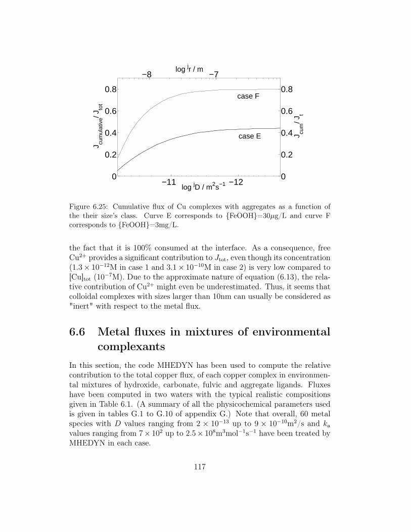
−12−110

0.2

0.4

0.6

0.8

log jD / m2s−1

Jcu

mul

ativ

e/ Jto

t

−8 −7

0

0.2

0.4

0.6

0.8

log jr / m

Jcu

m/ J

t

case E

case F

Figure 6.25: Cumulative flux of Cu complexes with aggregates as a function ofthe their size’s class. Curve E corresponds to FeOOH=30µg/L and curve Fcorresponds to FeOOH=3mg/L.

the fact that it is 100% consumed at the interface. As a consequence, freeCu2+ provides a significant contribution to Jtot, even though its concentration(1.3× 10−12M in case 1 and 3.1× 10−10M in case 2) is very low compared to[Cu]tot (10−7M). Due to the approximate nature of equation (6.13), the rela-tive contribution of Cu2+ might even be underestimated. Thus, it seems thatcolloidal complexes with sizes larger than 10nm can usually be considered as"inert" with respect to the metal flux.

6.6 Metal fluxes in mixtures of environmental

complexants

In this section, the code MHEDYN has been used to compute the relativecontribution to the total copper flux, of each copper complex in environmen-tal mixtures of hydroxide, carbonate, fulvic and aggregate ligands. Fluxeshave been computed in two waters with the typical realistic compositionsgiven in Table 6.1. (A summary of all the physicochemical parameters usedis given in tables G.1 to G.10 of appendix G.) Note that overall, 60 metalspecies with D values ranging from 2 × 10−13 up to 9 × 10−10m2/s and ka

values ranging from 7× 102 up to 2.5× 108m3mol−1s−1 have been treated byMHEDYN in each case.

117

As already seen in section 6.5, the fractal aggregates are assumed to be

Compound Water n 1 Water n 2pH 8 8

[CO2−3 ]tot 2×10−3M 2×10−3M

FS 2 mg/L 2 mg/LSolid concentration 3 mg/L 3 mg/L

FeOOH 30 µg/L 300 µg/L[Cu]tot 10−8M 3.5 ×10−7M

Table 6.1: Main parameters used for flux computations in waters n 1 and n 2.

formed by the assembly of non complexing solid subparticles on which acomplexing minor component which can be regarded as amorphous FeOOHis adsorbed. In the two tested cases, the roles of fulvics and aggregates areexpected to change, since i) the copper to fulvic ratio increases from watern 1 to n 2 i.e. the complexing strength of Cu2+ by fulvic significantly de-creases and ii) the overall concentration (and thus the complexing strength)of aggregate complexing sites increases in the same order. Note that thelimitations discussed above for equation (6.13) is still valid in the presentcalculations. This is the more so as the theory, developed in [86], has beenestablished for non complexing solution.The concentration profiles at the interface obtained in the two cases for eachspecies are similar to those obtained in sections 6.3 to 6.5 and will not begiven here. The time evolutions of the total fluxes were similar to those ob-tained with aggregates alone (figure 6.22), confirming that reaction diffusionwith aggregates is also the slow step in mixtures of aggregate and solubleligands, and that the overall time to reach a constant total flux should notbe too much larger than seconds to minutes in environmental systems. Asmentioned in section 6.5, steady-state for large size complexes may take ∼ 30minutes, but their contribution to the flux is negligible.In the mixtures, at steady-state, the distribution of lability degree jξ andindividual fluxes jJ of the fulvic complexes with respect to jK, is similarto those obtained under the same conditions with only fulvics in solution.The same observation is made for the distributions of jξ and jJ with respectto jr (or jD) for complexes with aggregates. Thus these results are not re-ported here. On the other hand, Figure 6.26 shows the cumulative fluxes,∑

jJ = f(jr) (see section 6.5.2) of complexes with aggregates only, for thetwo tested waters. Comparison of figures 6.25 and 6.26 is interesting: thecurves E (figure 6.25), F (figure 6.25), water n 1 (figure 6.26) and water n 2(figure 6.26) correspond to increasing complexing strengths of aggregates forCu2+. It can be seen that the aggregates which contribute the most to the

118

−13−12−11−100

0.001

0.002

0.003

0.004

0.005

0.006

log jD (m2s−1)

Jcu

mul

ativ

e/ Jto

t

water n°1

water n°2

Figure 6.26: Cumulative fluxes of complexes with aggregate only as a functionof the diffusion coefficients of the aggregate class, for waters n 1 and n 2. Curvewater n 1 corresponds to FeOOH=30 µg/L, while curve water n 2 correspondsto FeOOH=300 µg/L. Parameters: Water 1: [Cu]tot = 10−8M, FAtot = 2mgC/l, logK∗ = 12.5, [CO2−

3 ]tot = 2mM; Water 2: [Cu]tot = 3.5−7M, FAtot = 2mgC/l, logK∗ = 9.5, [CO2−

3 ]tot = 2mM. Other parameters in tables G.1 and G.6.

119

Species X Water 1[X]/[Cu]tot% JX (molm−2s−1) JX/Jtot%

Cu2+ 0.003 1.04 × 10−14 0.53CuOH and Cu(OH)2 0.065 6.03 × 10−14 3.05

CuCO3 and Cu(CO3)2 0.128 1.83 × 10−13 9.28∑

Cu-FS 97.50 1.70 × 10−12 86.9∑

Cu-Aggregate 2.317 2.54 × 10−15 0.19J 1.97 × 10−12 100

Jtot/Jlab% 1.44

Table 6.2: Steady-state values of fluxes and bulk concentrations normalised withCu2+

tot of the species present in waters 1. Other parameters: see figure 6.26

Species X Water 2[X]/[Cu]tot% JX (molm−2s−1) JX/Jtot%

Cu2+ 0.097 1.21 × 10−12 0.45CuOH and Cu(OH)2 0.164 8.19 × 10−12 3.02

CuCO3 and Cu(CO3)2 0.305 2.09 × 10−11 7.68∑

Cu-FS 33.14 2.38 × 10−10 87.5∑

Cu-Aggregate 66.49 1.59 × 10−12 0.58J 2.72 × 10−10 100

Jtot/Jlab% 14.9

Table 6.3: Steady-state values of fluxes and normalised bulk concentrations withrespect to Cu2+

tot of the species present in waters 2. Other parameters: see figure6.26

total flux are always those with jr ≤ 10nm, irrespective of complexationstrength. Thus, even though more data are desirable, these results stronglysuggest that the contribution of metal-aggregate complexes with size largerthan 10nm can be neglected on flux computations.Table 6.2 and 6.3 provides the steady-state values of free Cu2+, carbon-ato complexes (CuCO2−

3 and Cu(CO2−3 )2−

2 ), hydroxo-complexes (CuOH+ andCu(OH)2), fulvic complexes and aggregate complexes, and their proportionto the total flux, Jtot. It also provides for comparison, the proportion of thevarious types of complexes in the mixture and the ratio of Jtot/Jlab where Jlab

is the total flux which would be observed if all complexes were fully labile.Tables 6.2 and 6.3 show that, for the two cases, the overall flux is largely

dominated by the Cu-fulvic complexes. Amongst inorganic complexes, thecarbonate complexes, CuCO3 and Cu(CO3)2, are the most important underthe conditions used, but their contribution to the total flux remains marginal.Indeed, their bulk concentrations, in both water, are much less than 1% that

120

[Cu]tot and their contribution to the total flux is less than 10%.The contribution of aggregate complexes to the total flux is negligible inboth cases, which justifies the use of the approximate equation (6.13), sinceit provides an upper limit to the flux of aggregate complexes. The negligi-ble contribution of metal aggregates is worth emphasising, since complexingstrength of their sites have been increased by 10 and the total Cu concentra-tion is increased by 35, in water 2. As a consequence, the total concentrationof aggregate complexes, with respect to the total concentration of Cu, is2.17% for water 1 and 66.49% for water 2. Simultaneously, the complexationstrength of the fulvics decreases by a factor of 352 = 1225 due to the increaseof the metal/fulvic ratio by a factor of 35. Even though all these conditionsshould favour the contribution of aggregates to the overall flux compared tofulvics, these latter still dominate. This is due to their respective degree oflability: this latter decreases for aggregates in water 2 compared to water 1,due to the increase of complexing site concentration. On the opposite, thedegree of lability of fulvic complexes drastically increases in water 2, due tothe increase of the metal to ligand ratio.

6.7 Computational time: performance of MHE-

DYN

Table 6.4 provides an order of magnitude of the computer time which wasneeded to perform computations of sections 6.3 to 6.6. It can be seen that forsuch realistic aquatic mixtures, the computer time is not negligible even forthe conditions of planar diffusion which were used here. Thus the computertime needed for similar 3D simulations would be significantly larger. Im-provements in computation time can be done by appropriate tuning of someparameters of MHEDYN. For instance, the user can decide by himself/herselfthe best choice for the grid refinement factor, the size of the smallest gridand the number of time iterations for fast reactions by using the time split-ting method. To reduce the computational time, the grid refinement factorshould be increased, so that the number of discretization points of the do-main is reduced. Furthermore, it is possible to decrease the number of pointswithin each sub-grid. However, one should pay attention to get a sufficientnumber of points, in particular close to the consuming surface where themost important changes in concentration gradient occurs.Finally, faster computers than those used here can be employed and the nu-merical algorithm can be parallelised and distributed on many processors.This has been successfully performed for 3D computation in biofilms (See

121

Process Computational timeSimple Ligands ∼ minutes to hoursFulvic Acids ∼ hours

Suspended Particles ∼ 1 - 10 hoursMixture ∼ hours to 1 day

Table 6.4: Computational time on a Pentium 4, with 2 Ghz and 224 MB of RAM.

chapter 8).

6.8 Summary

In this chapter different complex processes taking place in aquatic systemshave been studied by flux numerical computation in order to extract informa-tion on bioavailability and biouptake on consuming surfaces. The attentionwas focused on simple ligands, fulvic substances and aggregate of particles.We have used a multiligand approach to study these processes. The resultsshowed that there is a complex relationship among site concentrations, themetal to ligand ratio, the equilibrium constants of the complexes, the labilityand the mobility of complexes with the flux contribution of each species.The applications studied allowed us to test the capabilities and the majorcharacteristic of MHEDYN. MHEDYN is a reliable numerical code that cancompute the flux and profile concentrations of any species in the transientand steady-state regime, in any geometry, with a very large number of lig-ands (limited only by computer time), with rate constants and diffusioncoefficients varying over many orders of magnitude, without requirement ofligand excess compared to metal. At the present time no equivalent code isavailable, hence we believe MHEDYN can be a useful tool for the communityof chemists in order to better understand the behaviour of chemical complexsystems.

122

Part III

3D systems.Physicochemical Validation andan Environmental Application

123

Chapter 7

Physicochemical validation

7.1 Overview

In this chapter we validate the numerical method, given in algorithm 3 atpage 68, for 3D applications by performing voltammetric simulations of aspherical microelectrode.In section 7.2 the consuming surface acts as a perfect sink, and only free M ispresent in solution (section 7.2.1) or a semilabile complex is present (section7.2.2). In section 7.2.3 the gain of computation time due to the use of thegrid refinement procedure is given for a typical voltammetric micro-electrodesensor.In section 7.3 the general Nernst conditions, equation (2.35) at page 22 isapplied at the consuming surface and an electrochemical technique, for mea-suring free metal ion concentration, is numerically modelled.

7.2 3D case: comparison of LBGK performance

without and with grid refinement

The application of the grid refinement is particularly useful for three dimen-sional problems where the computational cost can become very high andsometimes prohibitive even by running the simulations on supercomputers.This is shown below with a few examples well known in voltammetry, forwhich results can be compared to the exact solution. We consider only twosubgrids for all the 3D cases studied here. A schematic sketch of the geome-try and the strategy used to set up the subgrids, for 3D simulations, is shownin figure 7.1. We consider now a spherical electrode with bulk initial condi-tions, equation (2.28 page 21). The boundary conditions are the following:

125

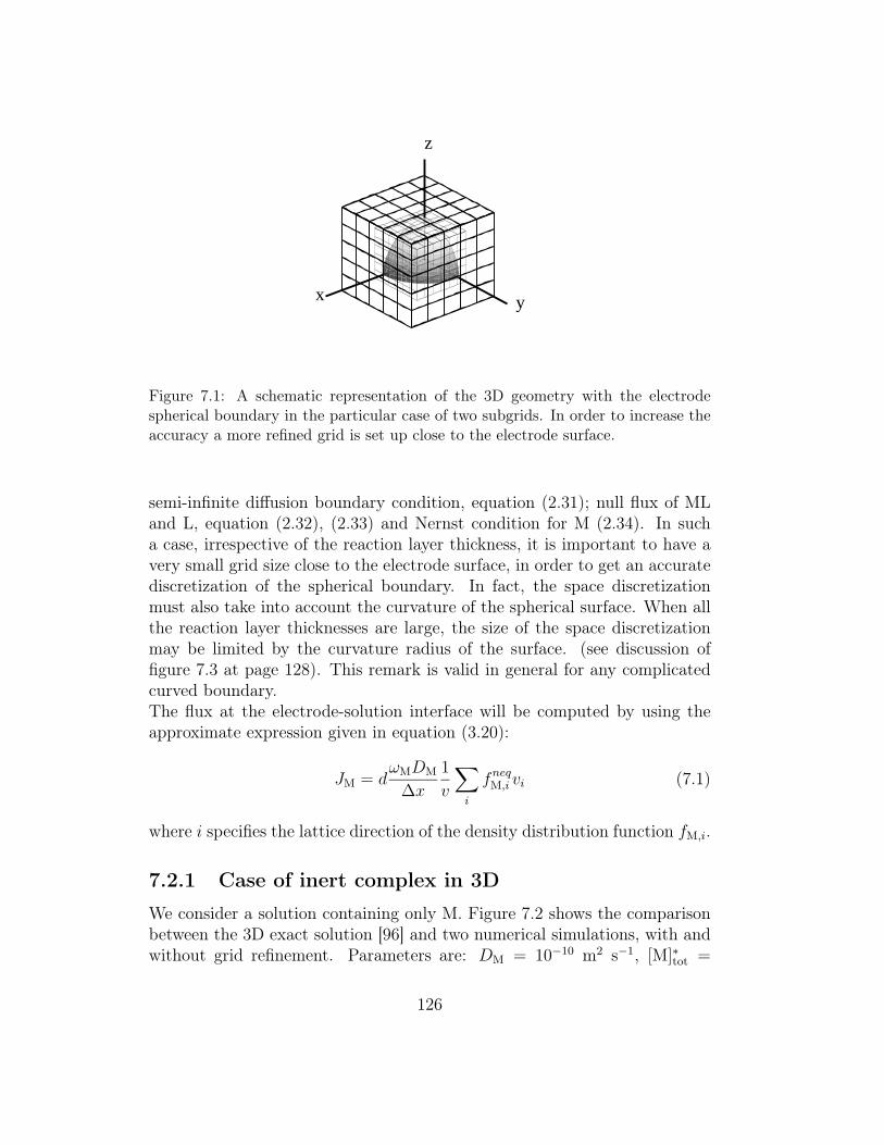
x y

z

Figure 7.1: A schematic representation of the 3D geometry with the electrodespherical boundary in the particular case of two subgrids. In order to increase theaccuracy a more refined grid is set up close to the electrode surface.

semi-infinite diffusion boundary condition, equation (2.31); null flux of MLand L, equation (2.32), (2.33) and Nernst condition for M (2.34). In sucha case, irrespective of the reaction layer thickness, it is important to have avery small grid size close to the electrode surface, in order to get an accuratediscretization of the spherical boundary. In fact, the space discretizationmust also take into account the curvature of the spherical surface. When allthe reaction layer thicknesses are large, the size of the space discretizationmay be limited by the curvature radius of the surface. (see discussion offigure 7.3 at page 128). This remark is valid in general for any complicatedcurved boundary.The flux at the electrode-solution interface will be computed by using theapproximate expression given in equation (3.20):

JM = dωMDM

∆x

1

v

∑

i

fneqM,i vi (7.1)

where i specifies the lattice direction of the density distribution function fM,i.

7.2.1 Case of inert complex in 3D

We consider a solution containing only M. Figure 7.2 shows the comparisonbetween the 3D exact solution [96] and two numerical simulations, with andwithout grid refinement. Parameters are: DM = 10−10 m2 s−1, [M]∗tot =

126

0 0.5 1 1.5 2 2.5 3x 10

−5

0

1

2

3

4

5x 10

−4

x (m)

cM

mol

/m3

inside theelectrode

G1 G

2

r0

Figure 7.2: Concentration profile of M in absence of ligand when the surface is aperfect sink. Comparison between the exact solution (dotted line), the numericalsimulations with grid refinement (x) and without grid refinement (o). Parametersare: DM = 10−10 m2 s−1, [M]∗ = 5 · 10−4 mol m−3, t = 0.5s, r0 = 8µm. Thesimulation without grid refinement is performed with ∆t = 10−3s and ∆x = 1µm,with 613 points and a computation time of ∼ 5minutes. The simulation with gridrefinement is performed with a lattice composed of two subgrids with n1 = 31 andn2 = 15, the same ∆t as without grid refinement, ∆x2 = ∆x and ∆x1 = ∆x

2 (gridrefinement g = 2). Computation time is ∼ 3minutes. Both simulations were runon a Pentium 4.

5 × 10−4 mol m−3, t = 0.5s, r0 = 8µm (r0 is the radius of the sphericalelectrode). The simulation without grid refinement is performed with ∆t =10−3s and ∆x = 1µm, while the simulation with grid refinement is performedwith the same ∆t, ∆x2 = ∆x in G2 and ∆x1 = ∆x

2in G1. The results

show that both numerical simulations are in good agreement with the exactsolution. The numerical discrepancy (of the order of a few percent) withthe exact concentration profile is only related to the discretization of theelectrode surface. Indeed, the sphere is not represented by a real sphere inthe discrete lattice, but as a summation of cubes. One way to overcomethis loss of precision is to consider a discretization which more exactly fitsthe boundary, i.e. the boundary points should exactly overlap the latticepoints. One proposition, discussed in [58], is to use off-lattice points in orderto exactly fit the required boundary values at the electrode surface.

127

0 10 20 30 40 50 60

5

10

15

20

25

30

35

40

45

50

55 0.5

1

1.5

2

2.5

3

3.5

4

4.5

x 10−4

a)0 0.1 0.2 0.3 0.4 0.5 0.6 0.7 0.8 0.9 1

x 10−3

0

0.5

1

1.5

2

2.5

3

3.5

4

4.5

5x 10−7

t (s)

J M (

mol

/m2 s)

b)

Figure 7.3: a) Concentration profile of M at z = 0 computed with grid refinement.b) Flux at the electrode computed without and with grid refinement comparedwith the numerical inversion of the analytical solution in the Laplace domain for aspherical electrode. Parameters: DM = DL = DML = 10−10 m2 s−1, ka = 100 m3

mol−1 s−1, kd = 100 s−1, r0 = 2.75µm, [M]∗tot = 10−3 mol m−3, [L]∗tot = 1 mol m−3.The simulation without grid refinement was run with ∆x = 0.1µm and ∆t = 10µs.The simulation with grid refinement was run with ∆x1 = ∆x, ∆x2 = 2∆x1, and∆t = 10µs. Legend: (continuous line) numerical inversion of analytical solutionin Laplace domain (see appendix B in [79]), (dashed line) scheme without gridrefinement, (marker +) scheme with grid refinement.

7.2.2 Semi-labile complex in 3D at a spherical electrode

Figure 7.3a) shows the contour plots of ML concentration obtained by ap-plying the grid refinement to a semi-labile complex ML in excess of ligandL. Parameters of the simulation are: DM = DL = DML = 10−10 m2 s−1,ka = 100 m3 mol−1 s−1, kd = 100 s−1, r0 = 2.75µm, [M]∗tot = 10−3 mol m−3,[L]∗tot = 1 mol m−3 and [ML]∗ = 5 × 10−4molm−3. Figure 7.3b) shows thefluxes computed with and without applying the grid refinement comparedwith the numerical inversion of the analytical solution in the Laplace domain(see appendix B in [79]). The simulation without grid refinement was runwith ∆x = 0.1µm and ∆t = 10µs. The simulation with grid refinement wasrun with ∆x1 = ∆x, ∆x2 = 2∆x1, ∆t = 10µs. Both fluxes obtained withand without grid refinement fit well the expected flux. As in section 7.2.1,we notice that the numerical flux is in both cases lower than the analyti-cal one. The reason of this negative discrepancy is due to the too roughdiscretization that we use to reproduce the spherical surface. In fact, thearea of the discretized surface is larger than that of the real surface and soit is reasonable that the flux computed is underestimated. The importantconclusion to highlight is that the grid refinement allows us to practicallypreserve the same accuracy on the flux computation with the advantage to

128

get a faster simulation. In the following section 7.2.3, we give the generalgain in computation time allowed by the application of the grid refinementmethod.

7.2.3 Gain of computation time in 3D with grid refine-ment

Figure 7.4 shows the computation times for the semilabile case discussed

30 80 130 180 230 28010

2

104

106

108

number of points in coarse grid

com

puta

tion

time

(sec

onds

)

Figure 7.4: Computation time as a function of the discretization for a sphericalelectrode of radius r0 = 20µm. Abscissas correspond to the number of points ofthe coarser grid. The refinement is placed at xs = 2µ, g = 5 and ∆x1 = µ/10.Markers: (*) Simulation with finer grid (strategy 1 in the text), (o) Simulation withcoarser grid (strategy 2 in the text), (+) Simulation with grid refinement (strategy3 in the text).

in the previous paragraph: DM = DL = DML = 10−10m2s−1, ka = 104

m3mol−1s−1, kd = 104s−1, [M]∗tot = 10−3 molm−1, [L]∗tot = 1 mol m−3, ∆x1 =µ = 0.1µm, ∆t = 10−5s and g = 5. The separation between the two subgridsis placed at xs = 2µ.Computations have been done with three strategies:

1. one grid with ∆x = ∆x1 = µ/10 and n1 points.

2. one grid with ∆x = ∆x2 = 5∆x1 and n2 points.

129

3. two subgrids with ∆x1 = µ/10, ∆x2 = 5∆x1, n1 points in subgrid G1

and n2 points in subgrid G2.

The results show that the gain in computation time, using strategy 3 com-pared to strategy 1, is nearly two orders of magnitude and that computationtimes of strategies 2 and 3 are almost the same, but, as seen before in figure7.2 at page 127, the accuracy of strategy 3 is slightly better.

7.3 AGNES simulation

In this section we consider the reduction of the metal M into its form M0 ata spherical electrode where it is amalgamated by fixing the ratio of M andM0 concentrations at the electrode surface by imposing a constant electricalpotential E at the electrode (see Nernst equation (2.35)). Figure 7.5 and 7.6show several plots of the concentration profiles of M and M0 registered atdifferent times by performing an AGNES like simulation.AGNES is an electroanalytical technique for measuring free metal ion con-centration. In the deposition stage of this technique a constant potentialis imposed at the electrode and the reduced metal is accumulated until theequilibrium is reached. This amount of metal is then measured (in the strip-ping step) by reoxidation and enables to compute the free M concentrationby using Nernst law. A more detailed description of the method is given in[97]. Here we limit ourselves to numerically reproduce the results of AGNES

for a fixed ratio [M0][M]

= Y = exp(

− nFRT

(E − E0))

, which corresponds to the

application of a fixed potential E in the Nernst equation. In our test, wehave fixed Y= 10. The radius of the spherical electrode is r0 = 2.5µm andfinite diffusion conditions are considered at r1 = 4µm, in other worlds, thesolution is supposed to be homogeneous at r = 4µm. The initial concentra-tions are: [M]∗ = 10−6M and [M0]∗=0. A finite volume condition is appliedat the centre of the electrode, at r = 0: ∂[M0]

∂r= 0.

Figure 7.5 shows the concentration profile of M at the plane z = 0, whilefigure 7.6 shows the concentration profile of M0. As shown in these figures,during the time evolution, the diffusion of M in solution and of M0 inside theelectrode converge to the prescribed ratio Y . As expected, the figures showthat, after 50ms, with the used parameters, the concentration profiles of Mand M0 becomes constant and such that [M0]

[M]= 10. This fast attainment

of a moderate gain (Y = 10) supports the convenience of (experimentally)investigating the use of microelectrodes for some implementation of AGNES.

130

020

4060

0

500

0.5

1

x 10−6

nx

ny

c M

020

4060

0

500

0.5

1

x 10−6

nx

ny

c M

020

4060

0

500

0.5

1

x 10−6

nx

ny

c M

020

4060

0

500

0.5

1

x 10−6

nx

ny

c M

020

4060

0

500

0.5

1

x 10−6

nx

ny

c M

020

4060

0

500

0.5

1

x 10−6

nx

ny

c M

t=0.25ms t=0.5ms

t=1ms t=2.5ms

t=5ms t=50ms

Figure 7.5: Plot of the concentration profile of M at several time at z = 0 (see figure7.1) of an AGNES simulation. Parameters are: [M0]/[M]=10 at r = r0, r0 = 2.5µm,r1 = 4µm. Initial concentrations are: [M]=[M]∗ = 10−6M and [M0]=0. Aftert = 50ms, [M] has practically achieved = 10−6M everywhere within the solution.The centre of the electrode is placed at nx = ny = 0.

131

020

4060

0

500

1

2

x 10−6

020

4060

0

500

1

2

x 10−6

020

4060

0

500

1

2

x 10−6

020

4060

0

500

2

4

x 10−6

020

4060

0

500

2

4

x 10−6

020

4060

0

500

0.5

1

x 10−5

t=0.25ms t=0.5ms

t=1ms t=2.5ms

t=5ms t=50ms

Figure 7.6: Plot of the concentration profile of M0 at several time at z = 0 (seefigure 7.1) of an AGNES simulation. Same parameters as in figure 7.5 After t =50ms, [M0] has practically achieved = 10−5M everywhere within the electrode. Thecentre of the electrode is placed at nx = ny = 0.

132

7.4 Summary

In this chapter we have successfully validated the numerical method sug-gested in this thesis for chemical systems in 3D geometry with a sphericalconsuming surface, either a sensor or a microorganism. The main conclusionof this chapter is that accurate computations of concentration profiles andmetal fluxes are obtained provided that the Cartesian grid near the sphericalsurface is sufficiently small compared to the curvature radius of the sphere.The validation was performed also for non complexed metal or semilabilecomplexes. The metal fluxes obtained show a very good agreement with theanalytical solution.

133

Chapter 8

Modeling Fluxes in a Biofilm

8.1 Overview

In this chapter a biofilm model is described and the numerical algorithmdiscussed at page 68 is applied to the biofilm model to compute metal fluxesat the microorganism surface within the biofilm. The chapter is organisedas follows. Section 8.2 describes in general what is a biofilm and the impor-tance of studying reaction-diffusion processes in such systems. Section 8.3discusses a typical biofilm model. Section 8.4 proposes a numerical procedurebased on the parallelisation of the numerical algorithm 3 at page 68. Finally,some examples of reaction-diffusion of complexes in biofilms, under differentlability conditions, are shown in section 8.5.

8.2 General description of a Biofilm

A biofilm can be seen as an organic gel layer of exopolymers attached to asurface and including microorganisms.Biofilms are highly diverse. They can range from a single cell on a surfaceto towers of several meters high and with diameter of 50 cm. They can bemade from bacteria, but can also include mussels or worms.A typical thickness of model biofilm, as studied in laboratory, is between 50and 1000 micron. Inside bacterial biofilm, the microorganism densities aretypically of the order of 1011 cells per millilitres. In general, bacteria cellscan be assumed to be 1 micron of diameter and they can be isolated or formclusters. Between the clusters, the biofilm exhibits openings, channels orpores. Through this channels, flow and transport of oxygen and substratesinto the biofilms are possible. Often, such pores have a volume similar tothose of clusters. Clusters may be about 200µm wide, or even smaller. Com-

135

prehensive reviews on biofilms are [98, 99, 100, 101].The study of trace metal transport in a biofilm is important from the en-vironmental point of view, because it will influence the overall activity ofthe biofilm. Rigorously, other effects should be considered. For instance,microbial transpiration may lead to a gradual pH decrease, of about 0.1−0.4units, while photosynthesis may lead to a pH increase of 1 − 3 units. Thismay strongly affect the binding of metals to biomass and exopolymers. Inanoxic zones, sulfate reduction will also lead to the production of sulfide,with obvious repercussions for metal transport.

Reaction-diffusion in Biofilms

As discussed above, many interacting processes take place in a biofilm. Thefollowing are particularly important [20]:

• Fluid flow over the biofilm surface

• Convection, diffusion and reaction inside the biofilm

• bacterial growth

• Biomass spreading and biofilm detachment due to biofilm deformationstress

Biomass growth and detachment rates are usually much slower than therate of diffusion into the biofilm. In fact, they have a time scale of theorder of 105s, while diffusion-reaction is of the order of 10-102 s, so the canbe considered at frozen processes. Hydrodynamics (momentum transportby convection or dissipation) over the biofilm surface is much faster thandiffusive mass transfer inside the biofilm. Therefore, the solution above thebiofilm can be considered as homogeneous.For those reasons, it is acceptable to solve separately the fluid flow field andthe reaction-diffusion processes.In this thesis we propose a new numerical algorithm based on algorithm 3 atpage 68 to solve reaction-diffusion systems inside a biofilm configuration asshown in figure 8.2.

8.3 A biofilm model

Based on the above discussion, we have chosen a very much simplified biofilmmodel, where pH and redox conditions are uniform and where the only chem-ical reaction considered is the complexation reaction M+L­ML.

136

We consider a cluster of bacteria inside a parallelepipedic section of a flatbiofilm covering an impenetrable surface. The bacteria inside the cluster havea random distribution. The bacterial layer is overtopped by an organic gellayer without bacteria. In this region, the pollutants (M,L) can diffuse to betaken by the organism in the cluster region. In the cluster, each bacteriumis a sphere with radius r0. Diffusion coefficients in the gel and in the clusterbetween the bacteria is assumed to be the same as in solution.Assuming a box cluster of 20 µm size and bacteria with radius r0 = 1µm, ifwe want to reproduce biofilm with maximum distance between bacteria fixedto 2r0, corresponding to a typical density of 1011 cells per millilitres, thenthe number of bacteria should be about 120. In our simulations, we haveconsidered 125 bacteria in the cluster. They are positioned randomly insidethe cluster. At the top of the cluster, the gel is 50µm high and is in contactwith a bulk homogeneous solution. Figure 8.1 shows the 3D picture of thebiofilm model and figure 8.2 shows a section of the biofilm model along theyz-plane, at x = 0. Note that, the vertical walls have periodic conditionsso that, with just a section of 20µm×20µm, we can simulate an indefinitebiofilm in the x and y directions. At the bottom end of the biofilm, corre-sponding to its substratum or support, a no-flux condition is fixed, while aconstant concentration is fixed at the upper end.

8.4 The numerical method: BIODYN

In this section we propose a numerical algorithm, that we call BIODYN.We consider, as starting point, the prototype reaction M+L­ML, in excessof ligand conditions. Therefore we can define a pseudo-association constantk′

a = ka[L]∗.

8.4.1 The method

The biofilm model we have introduced is decomposed in two regions: one iscalled the cluster region and the other one is called the gel region. As shownin figure 8.3, cluster and gel regions are separated by the plane z = z.In the region occupied by the bacteria and near the gel, the bacteria distri-bution locally influences the concentration of M and ML. However, movingupward far away from the cluster, its local influence on the concentrationsof M and ML decreases and the cluster can be considered more and moreas a homogeneous consuming surface. In other words, the overall diffusioninside the gel takes place mostly along the z direction, also due to the fact

137

Figure 8.1: The biofilm model, with 125 randomly distributed microorganisms,simulated in this section. The spherical microorganisms have radius r0 = 1µm. Thecluster region, where the microorganisms are present, is 20µm×20µm×20µm at thebottom of the parallelipipedic box. The gel region extends at the top for 50µm.The cluster is attached to an impenetrable, inert substrate and a homogeneousbulk solution is at the top of the gel layer. Periodic conditions are applied to thevertical walls so that the biofilm extends to infinity in the x and y directions.

138

Figure 8.2: Section at x = 0 of the biofilm model shown in figure 8.1, with theboundary conditions. At the bottom end a no-flux condition is imposed and con-stant concentration is fixed at zmax = 70µm.

139

Figure 8.3: Section of the biofilm at x = 0. The picture shows the interface ofseparation at z = z of 3D/1D and the interface where the 1D scheme and the 3Dscheme are applied, z = 3

2 z. The picture shows also the missing values of fX,i, thatare computed by adopting the method shown at the points 1 - 4 of section 8.4.2

140

that a homogeneous bulk concentration is fixed at z = zmax. Thus, planar1D diffusion can be applied to the top part of the gel.After some tests, in which we have computed the gradient of M and ML ateach point, along the three Cartesian directions, we have seen that at z = 3

2z

the concentration gradients of the species along x and y becomes negligibleand that planar 1D diffusion is applicable along the z direction. Therefore itseems reasonable to separate the computational domain into two parts. Inthe first part, P1 = 0 < z < 3

2z, we apply the complete 3D scheme given in

equation (3.7) page 28 with d = 3. In the second part P2 = 32z < z < zmax,

we apply the complete 1D scheme given in the same equation (3.7) at page28, with d = 1.This choice has two big advantages over a 3D simulations of the whole box:

1. The computational time is much faster.

2. The memory usage is considerably much lower

8.4.2 The condition at 3D - 1D interface

At the interface of separation between the 3D scheme defined in P1 and the1D scheme defined in P2, we have to determine the fX,i(x, t)-values missingfor the species X=M and ML. Let us suppose that we know the fX,i(x, t)at a given time t. Both schemes are defined at the interface of separation,z = 3

2z. By applying the numerical scheme in P1, we compute all the values

of fX,i(x, t) at t = t + ∆t, except for fX,6 at z = 32z . By applying the

numerical scheme in P2, we compute all the values of fX,i(x, t) at t = t+∆t,except for fX,5, at z = 3

2z. The missing values are computed in the following

way:

1. At z = 32z + ∆z we compute the average concentration c1

X.

2. At z = 32z − ∆z we compute the average concentration c2

X.

3. By linear interpolation, we compute the concentration of X at z = 32z,

such that: cX =c1X+c2X

2

4. This value is used to determine the missing density distribution func-tions by using the usual expression given in equation (3.16) at page30.

141

8.4.3 parallelisation of the code

The new numerical algorithm we suggest is a combination of 1D and 3DLattice Boltzmann method, coupled together, at constant z. For the reasonsexplained below, the 3D numerical algorithm applied in the domain P1 hasbeen translated in a parallel code. The 3D + 1D code used to solve reaction-diffusion processes in the biofilm is called BIODYN. It is described below.The 3D code on the domain P1 is very expensive in terms of computationaltime and memory usage. The reason is that we have to use a large numberof points to resolve correctly the spatial domain near and on the surface ofthe spherical microorganism. For instance, because microorganism size istaken as 1µm, the value of ∆x should be less or equal to 0.1µm to minimisethe error due to discretization at the organisms surface (see section 7.2). Inaddition, when µ ≤ 0.1µm, ∆x should even be smaller than 0.01µm.The application of the grid refinement here is not useful, since the averagedistance among microorganisms is ∼ a few micrometres.Another solution is to parallelise the code, running it on several processors.This allows us to i) reduce the time of CPU computation and ii) to split thememory all over the processors gaining significantly in memory use.It is not here the place to describe in detail the parallelisation procedure. Weonly give the essential ingredients.Starting from the algorithm 3 at page 68, we consider only one grid G.Let us suppose to know all the f ’s at time t. The first step is to split thedomain P1 into p equal subdomains P1,p along the z direction. The secondstep is to consider the p computational grids G p, all with the same ∆t and∆x, associated to each subdomains P1,p and to distribute each of them toa processor p. The third step is to apply the numerical code (collision andpropagation step) in each processor to get the values of f ’s at t + ∆t. Thispart of the parallelisation procedure is done independently by each processor,i.e. they all work at the same time. Fourth step is to apply the procedurefrom 1 to 4 of section 8.4.2 at the interface of separation z = 3

2z and finally

the fifth step is to update the values of f ’s at the boundary of each processor.This last step is the real limiting factor of the parallelisation process, becausein this step all the processors have to communicate with each other and theytransfer themselves the necessary information in order to be ready for thenew time step t+∆t. The numerical code BIODYN is described in algorithm4 at page 143.

142

Algorithm 4 Parallel algorithm to solve reaction diffusion processes inbiofilm: BYODIN code

SET UP of INITIAL CONDITIONSfX,i(x, t) at t = 0 on grid G

START of NUMERICAL SCHEMEt ← t + ∆twhile t ≤ tf do

Application of 1D scheme in the domain P2

COLLISION 1: DIFFUSIONApplication of equation (4.4)

COLLISION 2: REACTIONApplication of equation (4.5)

PROPAGATIONApplication of equation (4.6)

for all Processor p do*****************************************Application of 3D scheme in the domain P1

Step done independently by each processor pCOLLISION 1: DIFFUSION

Application of equation (4.4)COLLISION 2: REACTION

Application of equation (4.5)PROPAGATION

Application of equation (4.6)*****************************************

end forUPDATE AT INTERFACE 1D - 3D

Application of points 1 - 4 of section 8.4.2PROCESSOR BOUNDARY UPDATE

Update of the fX,i’s at the boundary of each processor pBOUNDARY CONDITIONS

Application of numerical boundary conditionsCOMPUTATION OF CONCENTRATION PROFILES

[X](x, t) =∑

i fX,i(x, t)FLUX COMPUTATION at the consuming surfacet ← t + ∆t

end while

OUTPUT RESULTSWriting of concentration profiles and flux

143

8.5 Metal fluxes in presence of the reaction M­ML

at different lability

8.5.1 Simulation conditions

In order to cover as many interesting cases as possible, the values of thephysicochemical parameters have been chosen in such a way that:

1. The lability index L varies from as labile as possible (L ∼ 1) to nonlabile (L ¿ 1). L is defined as [94]:

L ≡ Jkin

Jlab

(8.1)

where Jkin is the hypothetical maximum kinetic flux (without diffusionlimitation) and Jlab is the flux which would be obtained by using equa-tion (2.17) at page 17, if the complex was fully labile. In this work, weestimate Jkin via the computed actual flux J .

2. The association reaction layer, µML = DM

k′

a, varies from smaller than r0

(bacteria radius) to larger than cluster thickness (20 µm).

3. The dissociation reaction layer thickness, αML =√

DML

kd, varies in a

similar range.

For spherical diffusion, around isolated microorganisms, the lability index,Lm (where the subscript ’m’ stands for "microorganism"), is given by [94]:

Lm =

√

kd(1 + εK ′)

DML

r0

εK ′ (8.2)

An "overall" lability index, Lc (where the subscript ’c’ stands for "cluster"),can be computed for consumption of M by the whole cluster (considered asa single "organism") by considering that planar diffusion occurs in the gelabove the cluster. r0 is then replaced by the thickness of the gel, zmax − z:

Lc =

√

kd(1 + εK ′)

DML

zmax − z

εK ′ (8.3)

Note that in our biofilm, a given complex may be labile in the gel and nonlabile in the cluster or around an isolated microorganism, due to the factthat zmax − z À r0.

144

The choice of values of the lability index is not so trivial, because in additionto the above criteria, the condition K ′ > 1 should be maintained, DM, DML,k′

a and kd values should be realistic, and µML and αML should not be toodifferent from r0.Based on the above considerations, the lability index, Lm, the reaction layerthickness µML and αML are imposed and the other parameters are computedfrom them. The values of Lm and Lc, the association and dissociation rateconstants, k′

a and kd, the reaction layer thicknesses µML and αML and theequilibrium constant K ′ are summarised in table 8.1.The initial conditions are: [L]=[M]=[ML]=0 everywhere at t < 0, includingz > zmax. At t = 0, homogeneous total concentrations of M and L, [M]∗tot =10−6M and [L]∗tot = 10−3M, are imposed in the bulk solution, simulating anabrupt "pollution" increase of M and L.The boundary conditions are the following:

• At z = 0, the fluxes of M and ML are null.

• At z = zmax, the bulk (equilibrium) concentrations are applied (firsttwo columns of table 8.1).

• Periodic boundary conditions are applied at x = 0, x = xmax, y = 0and y = ymax.

• At the boundary of each bacterium, the Michaelis-Menten condition,given in equation (2.39) at page 23 is used. However, in all the sim-ulations shown here, we will consider a very fast internalisation rate,so that the volume concentration of the free metal M at the bacteriasurface is assumed to be null, i.e [M]=0. However, the code enables usto use any value of the Michaelis-Menten parameters.

The values of the diffusion coefficients are DM = 7× 10−10m2s−1 and DML =10−10m2s−1. The discretization parameters are ∆x = 2 × 10−7m and ∆t =10−4s in all the simulations.

8.5.2 Simulation results

Figures 8.4 and 8.5 show the concentration profiles of M and ML respectivelyfor the case 2 (see table 8.1) after t = 10s. As we can see the metal and

the complex concentrations are close to zero in the cluster region, due to tworeasons i) each microorganism behaves as a perfect sink and ii) complex isclose to labile, i.e. easily dissociated and consumed.The local value of the lability index on microorganism surface in the biofilm,

145

Figure 8.4: Contour plots of isoconcentrations of M in the biofilm region aftert = 10s for the case 2 (see table 8.1). In the cluster region the concentration of Mis very close to zero due to the perfect sink condition imposed at the microorganismsurface.

146

case 1 case 2 case 3 case 4 case 5[M]∗ (µM) 7.35 125 0.179 1.43 27.8

[ML]∗ (mM) 0.993 0.875 1.00 0.999 0.972k′

a (s−1) 2.80 × 105 7 × 102 2.80 × 105 7 × 102 1.75kd (s−1) 2070 100 50.1 1 0.050

K ′ 135 7 5590 700 35µML (µm) 0.05 1 0.05 1 20αML (µm) 0.2 1 2 10 45

Lm 1.06 1.41 0.03 0.01 0.01Lc 53.1 70.7 1.25 0.50 0.55

Table 8.1: Parameters used for the simulations: equilibrium concentrations of Mand ML in the bulk solution, association rate constant k′

a (s−1), dissociation rateconstant kd (s−1), equilibrium constant K ′ = K[L]∗, reaction layer thicknessesµML and αML (µm), lability indices Lm and Lc for isolated microorganism and thewhole cluster, respectively.

Figure 8.5: Contour plots of isoconcentrations of ML in the cluster region (0 < z <z) after t = 10s for the case 2 (see table 8.1).

147

0.5 1 1.5 20

0.5

1

1.5

2x 10−5

Lmb = J / J

lab

z (

m)

t = 10 s t = 20 s

Lm

Figure 8.6: The plot shows the lability index J/Jlab of each microorganism in thecluster as a function of its position z in the cluster. The plot corresponds to thecase 2 (see table 8.1) The corresponding value of Lm is shown for comparison.

Lbm, has been estimated by Lb

m = JJlab

computed at each microorganism sur-face. Jlab was obtained at each z by performing simulations with solutionscontaining the same value of [M]tot, but no ligand and using DML as diffusioncoefficient.As shown in figure 8.6, the values of Lb

m at each microorganism does notchange significantly from t = 10s to t = 20s, so we can consider to be al-ready practically at a pseudo steady-state at t = 10s for the whole biofilm.This fact justify the validity of the approximation of steady-state for theMichaelis-Menten condition. In fact, after typically 1-2 seconds, as shown in[33], the internalisation flux is already attained at a constant value and dΓ

dt

can be considered null.Figure 8.6 compares the values of Lb

m at each microorganism in the cluster,with the value of Lm for an isolated microorganism. It shows that in all casesLb

m < Lm. In addition, Lbm decreases with the depth in the cluster.

Figure 8.7 shows the local lability index, Lbm, at each microorganism for

the case 4 at t = 10s. Each value of Lbm is less (although not too much)

than the value of Lm (Lm = 0.01). Interestingly, again, all points at variousz values, are grouped on a straight line indicating that Lb

m slightly decreasewith depth. However, the points are more spread than those of figure 8.6.

148

10−4

10−3

10−2

10−1

1000

0.5

1

1.5

2x 10−5

Lmb = J / J

lab

z (

m)

Lm

Figure 8.7: The plot shows the lability index J/Jlab of each microorganism inthe cluster as a function of its position z in the cluster at t = 10s. The plotcorresponds to the case 4 (see table 8.1). The corresponding value of Lm is shownfor comparison.

An overall lability index for the cluster, Lctot, defined as:

Lctot =

∑

i Ji∑

i Ji,labile

(8.4)

has also been computed. In equation (8.4) Ji is the flux of M at each mi-croorganism i, and Ji,labile is the corresponding flux if the complex ML wasfully labile (equation (2.17) at page 17). It is found that Lc

tot = 6.8 × 10−3,i.e. a value close to the average of all values of figure 8.6.Figures 8.8, 8.9 and 8.10 show the lability index Lb

m of the microorganisminside the cluster for the case 1, 3 and 5 of table 8.1. They show the sameproperties than figures 8.6 and 8.7 with the exception that the lability indexLm < Lb

m only for the case 5. Furthermore, for the case 5, most of the labilityindexes of each microorganism are vertically aligned around a value which is∼ 2Lm. All the figures from 8.8 to 8.10 show that there is an average labilityindex of ML inside the cluster. In particular, each figure shows that the lo-cal lability indexes of each microorganism tend to align to this average locallability index with a dispersion that depends on the simulation conditions.It seems that the difference between Lb

m and Lm is related to the values ofthe reaction layer thicknesses µML and αML. Figure 8.6 shows a very smalldispersion of the values of Lb

m and the reaction layer thicknesses are equalto the microorganism’s radius (µML = αML = r0). On the other hand, figure

149

10−4

10−2

1000

0.5

1

1.5

2x 10−5

Lmb = J / J

lab

z (

m)

Lm

Figure 8.8: The plot shows the lability index J/Jlab of each microorganism inthe cluster as a function of its position z in the cluster at t = 7s. The plotcorresponds to the case 1 (see table 8.1). The corresponding value of Lm is shownfor comparison.

10−6

10−4

10−2

1000

0.5

1

1.5

2x 10−5

Lmb = J / J

lab

z (

m)

Lm

Figure 8.9: The plot shows the lability index J/Jlab of each microorganism inthe cluster as a function of its position z in the cluster at t = 7s. The plotcorresponds to the case 3 (see table 8.1). The corresponding value of Lm is shownfor comparison.

150

10−2

10−1

1000

0.5

1

1.5

2x 10−5

Lmb = J / J

lab

z (

m)

Lm

Figure 8.10: The plot shows the lability factor J/Jlab of each microorganism in thecluster as a function of its position z in the cluster at t = 10s. The plot correspondsto the case 5 (see table 8.1).

8.8 shows a very high dispersion and i) µML ¿ r0 and ii) αML < r0. Fur-thermore, figure 8.10 shows an intermediate dispersion of Lb

m and both µML

and αML are much larger than r0. It seems, thus that the more the reactionlayer thicknesses are close to r0, the more values of the local lability indexLb

m tend to align to a straight line and the dispersion is minimised. However,this behaviour must be checked with other simulations by choosing a widerspectrum of values of µML and αML.Figures 8.8, 8.6 and 8.9 show that the local lability index i) decreases withthe depth inside the cluster and ii) is much less than the lability index foran isolated microorganism. Instead, figures 8.7 and 8.10 show that the locallability is of the same order or larger than Lm. These facts suggest that thereis a correlation between the values of Lb

m as a function of the cluster depthand its average value. From our results, if Lb

m ≥ Lm then Lbm’s values are

aligned to a vertical straight line, while if Lbm ¿ Lm then the Lb

m’s valuesdecrease with the cluster depth. So, if Lb

m ≥ Lm the the local lability isconstant with the cluster depth.

151

8.6 Summary

In this section we have described a model of a simplified biofilm and we haveproposed a parallel code, BIODYN, to numerically simulate it. We haveperformed 5 different preliminary simulations with the same microorganismdistribution. From our results we can suspect that:

1. All the simulation conditions show the presence of an average locallability index of ML in the cluster.

2. The local lability index seems to decrease with the depth of the clusteror remain constant, depending on lability conditions.

3. It seems that, the more the reaction layer thicknesses are close to theradius of the bacteria, the more the local lability index Lb

m tend to alignto a straight line and the dispersion is minimised.

Furthermore, the method and the code developed in this chapter (BIODYN)can be coupled with others numerical codes to simulate others processes, likehydrodynamics and bacteria growth.

152

Chapter 9

Conclusions and Perspectives

9.1 Contributions

In this thesis we propose a new numerical algorithm, see page 68, based on theRegularised Lattice Boltzmann scheme for the first time applied to reaction-diffusion processes in chemically heterogeneous environmental systems. Wehave shown that, considering typical realistic values of the chemical rateconstants, the regularised LBGK scheme converges faster than the standardLBGK scheme and it also has a larger convergence domain.The systems investigated in this thesis belong to the class of the Multiscaleprocesses, due to the large variations of their physicochemical parameters.In order to numerically solve this kind of process, accurate methods shouldbe envisaged. Two well known techniques, useful for our problems, are thetime splitting methods and the grid refinement techniques.These two methods have been coupled with the regularised LBGK scheme.A summary of convergence results is given in figure 4.5 at page 71. We haveseen that:

• For the first time the time splitting method has been coupled with theRegularised Lattice Boltzmann scheme.

• The time splitting method breaks down a complicated problem intosmaller parts for the sake of time stepping, such that the different partscan be solved efficiently with suitable integration formulas. Specificallyfor reaction-diffusion problems, where the chemical reaction can be very’stiff’, smaller time steps or implicit methods can be used to solve onlythe reaction process.

• The grid refinement methods presented allows us to reduce the grid sizeof the domain only in regions where large gradient appears by decom-

153

posing the domain into several subgrids. This can reduce enormouslythe time of computations and the computer memory usage. On theother hand, the numerical scheme associated with the finer subgridcan be difficult to deal with the standard LBGK scheme, because itmay happen that, for large values of ω, the convergence criterion is notfulfilled anymore. This is solved by using the regularised approach.

The numerical algorithm developed in this thesis, has been transformed intwo program codes by using the Fortran 90 language: a) MHEDYN to solvemultiligand processes at planar consuming surfaces and b) BIODYN to solvethe simple complexation reaction M+L­ML in biofilm complex geometry.

1. MHEDYN - Multi Heterogeneous DYNamic. The features of MHE-DYN are:

(a) Computes metal fluxes at a planar consuming surface for paralleland unlimited successive complexation reactions of the metal M.

(b) Works with any ligand concentration value, i.e. both in excessand non excess compared to metal.

(c) Computes transient and steady-state metal fluxes and the degreeof lability of each complex.

(d) Computes transient and steady-state concentration profiles of allthe species present in solution.

(e) Works with a very wide range of physicochemical parameters.The code has been successfully applied to environmental systems(chapter 6) in the following conditions:

i. Diffusion coefficients of species varying from 2.4 × 10−13 to7.1 × 10−10 m2s−1

ii. Association constant of species varying from 7.2×102 to 2.5×108 m3mol−1s−1

iii. Equilibrium constant varying from logK = 4.1 to logK =16.1.

2. BIODYN - BIOfilm DYNamics. The features of BIODYN are:

(a) Computes metal fluxes and the local lability index at each bacteriasurface.

(b) Computes concentration profiles of each species in the biofilm do-main at transient and steady-state.

(c) Computes the accumulated metal in each bacterium.

154

(d) Works on several processors allowing to save computation timeand computer memory.

9.2 Perspectives

The proposed numerical algorithm can be improved in two directions:

1. The time splitting method allows us to separately solve the reactivepart from the diffusive part. One can in principle choose the bestnumerical scheme, to solve the reactive part, which for fast reaction,can become very ’stiff’. One solution is to use implicit schemes. Wehave only given a few examples in which we have applied the implicitscheme (see equation (4.7) at page 49). But we believe that this taskshould be studied in much more detail. However, for our applications,the explicit reactive scheme, given by equation (4.5) gives satisfactoryresults.

2. The Lattice Boltzmann scheme could be improved, avoiding the BGKapproximation described at page 27, by considering more general reac-tive schemes as described in [102], based on Lattice Gas Automata.

The results obtained in chapter 8 need to be checked more carefully bystudying the metal fluxes and the local lability index under different condi-tions. The first results show that the local lability index decreases with thedepth of the cluster or remains constant, depending on lability conditions inthe bulk. In addition, all the simulation conditions show the presence of anaverage local lability index of ML in the cluster and that it tends to align toa straight line when the reaction layer thickness of ML is close to the bacteriaradius.Furthermore, the method and the code developed in this chapter (BYODIN)might be coupled with others numerical codes to simulate others processes,like hydrodynamics and bacteria growth.

155

Bibliography

[1] J. Buffle and R. De Vitre. Chemical and biological regulation of aquaticsystems. Lewis Publishers, 1994.

[2] W. Koster and H.P. van Leeuwen. Physicochemical Kinetics and Trans-port at the Biointerface: Setting the Stage, chapter 1. John Wiley andSons, Ltd, 2004.

[3] W. (Ed) Stumm. Aquatic chemical kinetics. Wiley Interscience - NY,1990.

[4] H.P. van Leeuwen and J. Galceran. Physicochemical Kinetics andTransport at chemical-biological surfaces. IUPAC series on Analyticaland Physical Chemistry of Environmental Systems, chapter 3. JohnWiley and Sons, Chichester, U.K., Vol. 9, 2004.

[5] K.J. Wilkinson and J. Buffle. Critical Evaluation of PhysicochemicalParameters and Processes for Modelling the Biological Uptake of TraceMetals in Environmental (Aquatic) Systems, chapter 10. John Wileyand Sons, Ltd, 2004.

[6] J. Buffle. Complexation Reactions in Aquatic Systems. Ellis Horwood,Chichester, 1998.

[7] J. Buffle and Z. Zhang. Dynamic modelling of metal complexes in envi-ronmental multiligand systems. Critical evaluation of physicochemicalparameters and models for flux computation in presence of simple lig-ands, fulvic and particles. Environ. Sci. Technol., 2007.

[8] J. Heyrovsky and J. Kuta. Principles of Polarography. Academic Press,NY, 1966.

[9] J. Koutecky and J. Koryta. . Electrochim. Acta, 3:318–339, 1961.

157

[10] J. Buffle and M.L. Tercier-Waeber. Voltammetric environmental tracemetal analysis and speciation. From laboratory to in situ measure-ments. TrAC-Trends in Analytical Chemistry, 24:172–191, 2005.

[11] H.P. van Leeuwen. . Electroanal., 13:826–830, 2001.

[12] J. Galceran, J. Puy, J. Salvador, J. Cecilia, F. Mas, and J.L. Garces.Lability and mobility effects on mixtures of ligands under steady-stateconditions. Phys. Chem. Chem. Phys., 5:5091–5100, 2003.

[13] J. Salvador, J.L. Garces, J. Galceran, and J. Puy. Lability of a mix-ture of metal complexes under steady-state planar diffusion in a finitedomain. J. Phys. Chem. B, 110:13661–13669, 2006.

[14] J. Puy, J. Cecilia, J. Galceran, R.M. Town, and H.P. van Leeuwen.Voltammetric lability of multiligand complexes: the case of ML2. Jour-nal of Electroanalytical Chemistry, 571:121–132, 2004.

[15] J.D. Allison, D.S. Brown, and K.J. Novo-Gradac. Minteqa2/prodefa2,a geochemical assessment model for environmental systems: version3.0, user’s manual., 1991.

[16] I. Puigdomenech. Medusa: make equilibrium diagrams using sophisti-cated algorithms. windows program, 2001.

[17] J. Buffle, K. Startchev, and J. Galceran. Computing steady-state metalflux at microorganism and bioanalogical sensor interfaces in multili-gand systems. A reaction layer approximation and its comparison withthe rigorous solution. Accepted for publication in Phys. Chem. Chem.Phys., 2007.

[18] M.P. Harper, W. Davison, and W. Tych. DIFS–A modelling and sim-ulation tool for DGT induced trace metal remobilisation in sedimentsand soils. Environmental Modelling & Software, 15:55–66, 2000.

[19] J. Perez, C. Picioreanu, and M. van Loosdrecht. Modelling biofilm andfloc diffusion processes based on analytical solution of reaction-diffusionequations. Water Research, 39:1311–1323, 2005.

[20] C. Picioreanu, M.C.M. van Loosdrecht, and J.J. Heijnen. Proceedingsof the 8th International Symposium on Microbial Ecology. In C.R. Bell,M. Brylinsky, and P. Johnson-Grenn, editors, Microbial Biosystems:New Frontiers. Atlantic Canada Society for Microbial Ecology, Halifax,Canada, 1999.

158

[21] O. Wanner and W. Gujer. A Multispecies Biofilm Model. Biotechnol.Bioeng., 28:314–328, 1986.

[22] W. Rauch, H. Vanhooren, and P.A. Vanrolleghem. A simplified mixed-culture biofilm model. Water Research, 33:2148–2162, 1999.

[23] W. Hundsdorfer and I. Verwer. Numerical Solution of Time-DependentAdvection-Diffusion-Reaction Equations. Springer-Verlag Berlin Hei-delberg 2003, 2003.

[24] O. Filippova and D. Hanel. Grid Refinement for Lattice-BGK Models.Journal of Computational Physics, 147:219–228, 1998.

[25] B. Chopard and M. Droz. Cellular automata modeling of physical sys-tems. Cambridge University Press, 1998.

[26] S. Succi. The Lattice Boltzmann Equation. Oxford Science Publication,2001.

[27] X. Shan and H. Chen. Lattice Boltzmann model for simulating flowswith multiple phases and components. Physical Review E, 47(3), 1993.

[28] S. Chen and G. Doolen. Lattice Boltzmann Method for Fluid Flows.Annu. Rev. Fluid Mech., 30:329–364, 1998.

[29] D.A. Wolf-Gladrow. Lattice-Gas Cellular Automata and Lattice Boltz-mann Models. An introduction. Springer-Verlag Berlin Heidelberg,2000.

[30] S.P. Dawson, S. Chen, and G.D. Doolen. Lattice Boltzmann compu-tations for Reaction-Diffusion equations. Journal of Chemical Physics,98(2):1514–1523, 1993.

[31] J. Heyrowsky and J. Kuta. Principles of Polarography. Academic Press,1966.

[32] J. Buffle and G. Horvai. In situ monitoring of aquatic systems. Wiley,2000.

[33] J. Galceran and H.P. van Leeuwen. Dynamics of Bioupatke Processes:the Role of Transport, Adsorbtion and Internalization, chapter 4. JohnWiley and Sons, Ltd, 2004.

[34] B. Chopard and A. Dupuis. A mass conserving boundary conditionsfor lattice boltzmann models. In LGA2002, 2002.

159

[35] d’Humieres, D. and Ginzburg, I. and Krafczyk, M. and Lallemand, P.and Luo, L.-S. Multiple-relaxation-time Lattice Boltzmann Models in3D. Technical report, NASA/CR-2002-211660 - ICASE Report No.2002-20, 2002.

[36] Shan, X. and Doolen, G. Diffusion in a multi-component Lattice Boltz-mann Equation model. Technical report, Theoretical Division, LosAlamos National Laboratory, Los Alamos, NM 87545, 2002.

[37] X. He, L.-S. Luo, and M. Dembo. Some Progress in Lattice BoltzmannMethod. Part 1. Nonuniform Mesh Grids. Journal of ComputationalPhysics, 129:357–363, 1996.

[38] A. Masselot and B. Chopard. A lattice Boltzmann model for particletransport and deposition. Europhysics Letters, 42(3):259–264, 1998.

[39] B. Chopard, P. Luthi, and A. Masselot. Cellular automata and lat-tice boltzmann techniques: An approach to model and simulate complexsystems. World Scientific Publishing Company, 1998.

[40] X. He and G. Doolen. Lattice Boltzmann Method on Curvilinear Co-ordinates System: Flow around a Circular Cylinder. Journal of Com-putational Physics, 134:306–315, 1997.

[41] S. Chen, S.P. Dawson, G.D. Doolen, D.R. Janecky, and A. Lawniczak.Lattice Methods and their Applications to Reacting Systems. Comput-ers chem. Engng, 19(6/7):617–646, 1995.

[42] X. He and N. Li. Lattice Boltzmann simulation of electrochemicalsystems. Computer Physics Communications, 129:158–166, 2000.

[43] Q. Li, C. Zheng, N. Wang, and B. Shi. LBGK Simulations of TuringPatterns in CIMA Model. Journal of Scientific Computing, 16(2):121–134, 2001.

[44] G.S. O’Brien, C.J. Bean, and F. McDermott. A comparison of pub-lished experimental data with a coupled lattice Boltzmann-analyticadvection-diffusion method for reactive transport in porous media.Journal of Hydrology, 268:143–157, 2002.

[45] O. Dardis and J. McCloskey. Lattice Boltzmann scheme with realnumbered solid density for the simulation of flow in porous media.Phisical Review E, 57(4), 1998.

160

[46] J. Bernsdorf, U. Jaekel, T. Zeiser, S. Doi, T. Takei, H. Matsumoto,and K. Nishizawa. Numerical Simulation of Reaction-Diffusion andAdsorption Processes in Porous Media using Lattice Boltzmann Meth-ods with Concurrent Visualization. In K. Matsuno, A. Ecer, J. Pe-riaux, N. Satofuka, and P. Fox, editors, Parallel Computational FluidDynamics - New Frontiers and Multi-Disciplinary Applications, pages233–240. Elsevier Science B.V., 2003.

[47] Y.-S. Xu, Y.-J. Zhong, and G.-X. Huang. Lattice Boltzmann Methodfor Diffusion-Reaction-Transport Processes in Heterogeneus PorousMedia. Chin. Phys. Lett., 21(7), 2004.

[48] D. Britz. Digital Simulation in Electrochemistry. Springer-VerlagBerlin, 1988.

[49] L.K. Bieniasz. A Fourth-Order Accurate, Numerov-Type, Three-PointFinite-Difference Discretization of Electrochemical Reaction-DiffusionEquations on Non-Uniform (Exponentially Expanding) Spatial Grids inOne-Dimensional Space Geometry. J. Comput. Chem., 25:1515, 2004.

[50] M. Rudolph. Digital simulation with the fast implicit finite difference(FIFD) algorithm. Part 5: Digital simulations of square wave voltam-metry for any user defined. Journal of Electroanalytical Chemistry,502:138–145, 2001.

[51] J. Galceran, D.J. Gavaghan, and Rollett J.S. Two-dimensional imple-mentation of the finite element method with singularity correction fordiffusion limited current at an unshielded disc electrode. Journal ofElectroanalytical Chemistry, 394:17–28, 1995.

[52] J. Puy, J. Galceran, J. Salvador, J. Cecilia, J.M. Diaz-Cruz, M. Este-ban, and F. Mas. Voltammetry of labile metal-macromolecular systemsfor any ligand-to-metal ratio, including adsorption phenomena. Therole of the stability constant. Journal of Electroanalytical Chemistry,374:223–234, 1994.

[53] J. Josserand, J. Morandini, H.J. Lee, R. Ferrigno, and H.H. Girault.Finite element simulation of ion transfer reactions at a single micro-liquid | liquid interface supported on a thin polymer film. Journal ofElectroanalytical Chemistry, 468:42–52, 1999.

[54] F.L. Qiu and A.C. Fisher. The boundary element method: applicationsto steady-state voltammetric simulations within domain extending toinfinity. Electrochemistry Communications, 3:117–121, 2001.

161

[55] M. Junk. A finite Difference Interpretation of the Lattice BoltzmannMethod. Numer. Methods Partial Differential Eq., 17:383–402, 2001.

[56] T. Toffoli and N. Margolus. Invertible cellular automata: A review.Physica D, 45:229–253, 1990.

[57] P. Albuquerque, D. Alemani, B. Chopard, and P. Leone. Coupling aLattice Boltzmann and a Finite Difference Scheme. In M. Bubak, G.D.van Albada, P.M.A. Sloot, and J.J. Dongarra, editors, ComputationalScience - ICCS 2004: 4th International Conference, Kraków, Poland,June 6-9, 2004, Proceedings, Part IV, volume 3039, page 540. SpringerBerlin / Heidelberg, 2004.

[58] D. Alemani, B. Chopard, J. Galceran, and J. Buffle. Time splittingand grid refinement methods in the Lattice Boltzmann framework forsolving a reaction-diffusion process. In V.N. Alexandrov, G.D. vanAlbada, P.M.A. Slot, and J.J. Dongarra, editors, Proceedings of ICCS2006, Reading, LCNS 3992, pages 70–77. Springer, 2006.

[59] P. Bouillot. Méthode Lattice Boltzmann avec régularisation, appliquéeà la diffusion. Master’s thesis, University of Geneva, 2005.

[60] J.W. Thomas. Numerical Partial Differenetial Equations - Finite Dif-ference Methods. Springer-Verlag NY, 1995.

[61] L.J. Durlofsky, Y. Efendiev, and V. Ginting. An adaptive local-globalmultiscale finite volume element method for two-phase flow simulations.Advances in Water Resources, 30:576–588, 2007.

[62] M. Parvazinia and V. Nassehi. Multiscale finite element modeling ofdiffusion-reaction equation using bubble functions with bilinear andtriangular elements. Computer Methods in Applied Mechanics and En-gineering, 196:1095–1107, 2007.

[63] Y. Efendiev and T. Hou. Multiscale finite element methods for porousmedia flows and their applications. Applied Numerical Mathematics,2006. In press.

[64] M. Bajaj, P. Bhat, J. Prakash, and M. Pasquali. Multiscale simula-tion of viscoelastic free surface flows. Journal of Non-Newtonian FluidMechanics, 140:87–107, 2006.

[65] Y. Efendiev, V. Ginting, T. Hou, and R. Ewing. Accurate multiscalefinite element methods for two-phase flow simulations. Journal of Com-putational Physics, 220:155–174, 2006.

162

[66] P. Ming and X. Yue. Numerical methods for multiscale elliptic prob-lems. Journal of Computational Physics, 214:421–445, 2006.

[67] D. Yu, R. Mei, and W. Shyy. A multi-block lattice Boltzmann methodfor viscous fluid flows. Int. J. Numer. Meth. Fluids, 39:99–120, 2002.

[68] D. Yu and S.S. Girimaji. Multi-block Lattice Boltzmann method: Ex-tension to 3D and validation in turbulence. Physica A: Statistical Me-chanics and its Applications, 362:118–124, 2006.

[69] Y.S. Lian and K. Xu. A Gas-Kinetic Scheme for Multimaterial Flowsand Its Application in Chemical Reactions. Journal of ComputationalPhysics, 163:349–375, 2000.

[70] N. Yanenko. Methodes a pas fractionnaire. Libraire Armand ColinParis, 1968.

[71] D. Ropp, J. Shadid, and C. Ober. Studies of accuracy of time inte-gration methods for reaction-diffusion equations. Journal of Computa-tional Physics, 194:544–574, 2004.

[72] I. Alonso-Mallo, B. Cano, and J. C. Jorge. Spectral-fractional stepRunge-Kutta discretizations for the initial boundary value problemswith time dependent boundary conditions. Mathematics of Computa-tion, 73:1801–1825, 2004.

[73] W. Hunsdorfer and Verwer J.G. Numerical solution of Time-Dependent Advection-Diffusion-Reactions Equations. Springer-VerlagBerlin, 2003.

[74] H. De Jong and H. Leeuwen. Voltammetry of metal complex systemswith different diffusion coefficients of the species involved: Part I. Ana-lytical approaches to the limiting current for the general case includingassociation/dissociation kinetics. Journal of Electroanalytical Chem-istry, 234:1–16, 1987.

[75] A. Dupuis and B. Chopard. Theory and applications of an alternativeLattice Boltzmann grid refinement algorithm. Physical Review E, 67,2003. 066707.

[76] L.K. Bieniasz. Use of Dynamically Adaptative Grid Techniques for theSolution of Electrochemical Kinetic Equations. Part 1. J. Electroanal.Chem., 360:119, 1993.

163

[77] L.K. Bieniasz. Use of Dynamically Adaptative Grid Techniques for theSolution of Electrochemical Kinetic Equations. Part 2. J. Electroanal.Chem., 374:1, 1994.

[78] L.K. Bieniasz. Use of Dynamically Adaptative Grid Techniques for theSolution of Electrochemical Kinetic Equations. Part 3. J. Electroanal.Chem., 374:23, 1993.

[79] D. Alemani, B. Chopard, J. Galceran, and J. Buffle. Two grid re-finement methods in the Lattice Boltzmann framework for reaction-diffusion processes in complex systems. Phys. Chem. Chem. Phys.,8:4119–4130, 2006.

[80] E.R. Brown and R.F. Large. Techniques of Chemistry, Vol. 1, Part IIA, "Electrochemical Methods", chapter 6. Wiley, NY, 1971.

[81] K.J. Hollenbeck. INVLAP.m: A matlab function for numeri-cal inversion of Laplace transforms by the De Hoog algorithm,http://www.isva.dtu.dk/staff/karl/invlap.htm.

[82] J. Salvador, J. Puy, J. Galceran, , J. Cecilia, R.M. Town, and H.P. vanLeeuwen. Lability Criteria for Successive Metal Complexes in Steady-State Planar Diffusion. J. Phys. Chem. B, 110:891–899, 2006.

[83] J. Buffle and Z. Zhang. Dynamic metal speciation and flux computa-tion in environmental system. Critical evaluation and compilation ofphysico-chemical parameters for simple ligands, fulvics and particles.Submitted to Env. Sci. Technol., 2007.

[84] R.M. Fuoss. . J. Ann. Chem. Soc., 80:5059, 1958.

[85] J. Duval, K.J. Wilkinson, H.P. van Leeuwen, and J. Buffle. Humicsubstances are soft and permeable: evidence from their electrophoreticmobilities. Environ. Sci. Technol., 39:6435–6445, 2005.

[86] J.P. Pinheiro, M. Minor, and H.P. van Leeuwen. Metal SpeciationDynamics in Colloidal Ligand Dispersion. Langmuir, 21:8635–8642,2005.

[87] Released by USEPA in 1999. Visual MINTEQ: Web page =http://www.lwr.kth.se/English/OurSoftware/vminteq/.

164

[88] J.R. Lead, K.W. Wilkinson, K. Starchev, S. Canonica, and J. Buffle.Determination of diffusion coefficients of humic substances by fluores-cence correlation spectroscopy: role of solution conditions. Environ.Sci. Technol., 34:1365–1369, 2000.

[89] R.S. Altmann and J. Buffle. The use of differential equilibrium func-tions for interpretation of metal binding in complex ligand systems: itsrelation to site occupation and site affinity distributions. Geochimicaet Cosmochimica Acta, 52:1505–1519, 1988.

[90] J. Buffle, R.S. Altmann, and M. Filella. Effect of physico-chemicalheterogeneity of natural complexants. Part II: Buffering action androle of their background sites. Analytica Chimica Acta, 232:225–237,1990.

[91] J. Buffle, M. Filella, and R.S. Altmann. Polyfunctional description ofmetal complexation by natural organic matter: theory and practice. InBinding models concerning natural organic substances in performanceassessment, pages 149–161. Nuclear Energy Agency Organisation forEconomic co-operation and development, 1994.

[92] D.A. Dzombach and Morel F.M.M. Surface complexation modelling.Hydrous Ferric Oxide. Wiley Interscience, N.Y., 1990.

[93] Filella M. and J. Buffle. Factors controlling the stability of submicroncolloids in natural waters. Colloids and Surfaces A: Physicochemicaland Engineering Aspects, 73:255–273, 1993.

[94] H.P. van Leeuwen, R.M. Town, J. Buffle, R. Cleven, W. Davison,J. Puy, W.H. van Riemsdijk, and L. Sigg. Dynamic speciation anal-ysis and bioavaialability of metals in aquatic systems. Environ. Sci.Technol., 39:8545–8585, 2005.

[95] J. Galceran, J. Puy, J. Salvador, J. Cecilia, and H.P. van Leeuwen.Voltammetric lability of metal complexes at spherical microelectrodeswith various radii. Journal of Electroanalytical Chemistry, 505:85–94,2001.

[96] A.J. Bard and L.R. Faulkner. Electrochemical Methods: Foundamentalsand Applications. J. Wiley NY, 1980.

[97] J. Galceran, E. Companys, J. Puy, J. Cecilia, and J.L. Garces. AGNES:a new electroanalytical technique for measuring free metal ion concen-tration. Journal of Electroanalytical Chemistry, 566:95–109, 2004.

165

[98] J.W. Costerton, Z.L. Lewandowsky, D. De Beer, D. Caldwell, D. Ko-rber, and G. James. Biofilms, the customized microniche. J. Bact.,176:2137–2142, 1994.

[99] L. Hall-Stoodley, J.W. Costerton, and P. Stoodley. Bacterial biofilms:from the natural environment to infectious diseases. Nature Reviews,2:95–108, 2004.

[100] P. Stoodley, S. Yang, H. Lapin-Scott, and Z. Lewandowski. Rela-tionship between mass transfer coefficient and liquid flow velocity inheterogeneous biofilms using microelectrodes and confocal microscopy.Biotechnol. Bioeng., 56:618–628, 1997.

[101] D. DeBeer and P. Stoodley. Relation between the structure of an aer-obic biofilm and transport phenomena. Wat. Sci. Technol., 32:11–18,1995.

[102] J.P. Boon, D. Dab, R. Kapral, and A. Lawniczak. Lattice Gas Au-tomata for Reactive Systems. Physics Reports, 273:55–147, 1996.

[103] C. Cercignani. The Boltzmann Equation and Its Applications. Springer-Verlag NY, 1987.

[104] L.-S. Luo. Theory of the Lattice Boltzmann Equation. Technical report,ICASE, MS 132C, NASA Langley Research Center, 3 West Reid Street,Building 1152, Hampton, Virginia 23681-2199, USA, 2000.

[105] X. He and L.S. Luo. Theory of the lattice boltzmann method: fromthe boltzmann equation to the lattice boltzmann equation. PhysicalReview E, 56:6811–6817, 1997.

[106] V. Comincioli. Analisi Numerica. Mc-Graw Hill Milano, 1995.

[107] M. Renardy and R.C. Rogers. An Introduction to Partial DifferentialEquations. Springer-Verlag New York, 1992.

166

Appendix

167

Appendix A

The derivation of thereaction-diffusion equation fromthe Lattice Boltzmann equation

In this appendix the following simple reaction-diffusion equation

∂c

∂t= D∇2c − R (A-1)

written for the concentration c(x, t) of one species in the open set Ω ⊂ Rn

for n = 1, 2, 3, is obtained by applying the Chapman-Enskog procedure tothe lattice Boltzmann evolution equation:

fi(x + ∆xi, t + ∆t) = fi(x, t) + ω(f eqi (x, t) − fi(x, t)) + ∆t

R(x, t)

2d(A-2)

where R is the reaction term, D is the diffusion coefficient of the species.Good references where to find a detailed description of the Chapman-Enskogmethod are [103, 104, 26, 105, 39].The procedure is explained in detail step by step for a d dimensional problem.In particular, the expression for the zeroth, first and second order of thedensity distribution functions are carefully derived under assumptions onthe spatial and time scales.

A.1 Setting up the scene

The domain Ω is discretized with a grid size ∆x along all the 2d Cartesiandirections. The time step is fixed to be ∆t. The lattice velocities vi are

169

defined as:

vi =(

(−1)i+1 ∆x

∆t, 0 , 0

)

i = 1, 2 (A-3)

vi =(

0 , (−1)i+1 ∆x

∆t, 0

)

i = 3, 4 (A-4)

vi =(

0 , 0 , (−1)i+1 ∆x

∆t

)

i = 5, 6 (A-5)

The relationship between the lattice velocities vi and the time step ∆t canbe put in vector form ∆xi = vi∆t.The lattice velocities have to satisfy two lattice constraints: first, the lat-tice symmetry

∑2di=1 vi = 0 and second there should exist a constant C such

that∑2d

i=1 viαviβ = Cδαβ. The Greek indices label the spatial dimensionand i = 1, . . . , 2d. The definition of the lattice given in the equations (A-3),(A-4) and (A-5) satisfy the above mentioned two constraints. In particular,the lattice symmetry holds and the second constraint holds if C = 2∆x2

∆t2.

Note that the constant C depends on the grid size and on the time step.Care should be taken when one works with several grids because the Latticeevolution equation depends on the grid sizes. Hence, it is advisable to par-titioning the whole domain into sub-grids instead of use grids with variablestep.

A.2 The Chapman-Enskog procedure

Let fii=1,...,2d, be the density distribution functions such that fi : Rd ×

R → R. The basic idea in the Chapman-Enskog method is to develop thedensity distribution functions fi, the reaction rate R and the spatial and timederivatives around a small parameter ε and to compare the ε order obtainedby substituting them into the kinetic equation developed in space and timearound (x,t) with the Taylor expansion.The ε order of the development of each term is labelled with a superscript inparenthesis. Hence:

fi = f(0)i + εf

(1)i + ε2f

(2)i (A-6)

R = R(0) + εR(1) + ε2f(2)i (A-7)

are the expansion of fi and R around the small parameter ε, while the de-velopment of the space and time differential operators is the following:

∂x = ∂(0)x + ε∂(1)

x + ε2∂(2)x (A-8)

∂t = ∂(0)t + ε∂

(1)t + ε2∂

(2)t (A-9)

170

The above developments have to satisfy the following constraint:

ρ =∑

i

fi =∑

i

f(0)i (A-10)

and∑

i

f(k)i = 0 k ≥ 1 (A-11)

The expression of the density distribution functions for i = 1 at zero, first andsecond order in the small parameter ε are derived in the following proposition1.

Proposition 1 1Determination of f(0)1 , f

(1)1 and f

(2)1

1. If R(0) = 0, ∂(0)x = 0 and ∂

(0)t = 0 then

f(0)1 = f

(eq)1 (A-12)

2. Under the same hypothesis of 1 and if ∂(1)t = 0 and R(1) = 0 then

f(1)1 = −∆x

ω∂(1)

x f eq1 (A-13)

3. Under the same hypothesis of 1 and 2 the expression for f(2)1 is

f(2)1 =

∆x2

ω2∂(1)2

x feq1 − ∆x

ω∂(2)

x feq1 − ∆t

ω∂

(2)t feq

1 − ∆x2

2ω∂(1)2

x feq1 +

∆t

2ωdR(2)

(A-14)

Proof In order to analyse the different ε orders, the local Taylor expansion inspace and time at (x, t) in a right neighbour (x + v1∆t, t + ∆t) is needed up tosecond order ∆x and ∆t:

f1(x + v1∆t, t + ∆t) = f1(x, t) + ∆x∂xf1(x, t) + ∆t∂tf1(x, t)+

+∆x∆t∂x∂tf1(x, t) + ∆x2∂2xf1(x, t) + ∆t2∂2

t f1(x, t)(A-15)

By comparing the Taylor expansion, equation (A-15), with the Lattice Boltzmannequation, equation (A-2), the following expression is achieved:

ω(f eqi (x, t) − fi(x, t)) + ∆t

R(x, t)

2d=

= ∆x∂xf1(x, t) + ∆t∂tf1(x, t)+

+∆x∆t∂x∂tf1(x, t) + ∆x2∂2xf1(x, t) + ∆t2∂2

t f1(x, t)

(A-16)

1The notation ’Proposition’ is often used in mathematical book to state a characteri-sation of a property that requires a demonstration.

171

By substituting in the above expression the equations (A-6), (A-7), (A-8) and (A-9)one gets:

0 = ε0[

− ∆t

2dR(0) − ωfeq

1 + ωf(0)1 + ∆x∂(0)

x f(0)1 + ∆t∂

(0)t f

(0)1 +

+∆x(0)∆t(0)f(0)1 +

∆x2

2∂(0)2

x f(0)1 +

∆t2

2∂

(0)t

]

+

+ε1[

− ∆t

2dR(1) + ωf

(1)1 + ∆x∂(0)

x f(1)1 + ∆x∂(1)

x f(0)1 + ∆t∂

(0)t f

(1)1 +

+∆t∂(1)t f

(0)1 + ∆x∆t∂(0)

x ∂(1)t f

(0)1 + ∆x∆t∂(1)

x ∂(0)t f

(0)1 + 2

∆x2

2∂(0)

x ∂(1)x f

(0)1

]

+

+ε2[

− ∆t

2dR(2) + ωf

(2)1 + ∆x∂(0)

x f(2)1 + ∆x∂(1)

x f(1)1 + ∆x∂(2)

x f(0)1 +

+∆t∂(0)t f

(2)1 + ∆t∂

(1)t f

(1)1 + ∆t∂

(2)t f

(0)1 + ∆x∆t∂

(0)t ∂

(0)t f

(2)1 +

+∆x∆t∂(1)x ∂

(0)t f

(1)1 + ∆x∆t∂(2)

x ∂(0)t f

(0)1 + ∆x2∂(0)

x f(2)1 +

∆x2

2∂(1)2

x f(0)1 +

+2∆x2∂(0)x ∂(1)

x f(1)1 + 2∆x2∂(0)

x ∂(2)x f

(0)1 + ∆t2∂

(0)t f

(2)1 + ∆t2∂

(1)t f

(0)1 +

+2∆t2∂(0)2

t f(0)1 + 2∆t2∂

(0)t ∂

(1)t f

(1)1 + 2∆t(2)∂

(0)t ∂

(2)t f

(0)1

]

(A-17)

At the zeroth order in ε, if R(0) = 0, ∂(0)x = 0 and ∂

(0)t = 0, then:

f(0)1 = feq

1 (A-18)

At the first order in ε, if ∂(1)t = 0 and R(1) = 0 (and clearly R(0) = 0, ∂

(0)x = 0 and

∂(0)t = 0), then

f(1)1 = −∆x

ω∂(1)

x feq1 (A-19)

With the same hypothesis as above (R(0) = ∂(0)x = ∂

(0)t = ∂

(1)t = R(1) = 0) the f

(2)1

is:

f(2)1 =

∆t

2ωR(2) − ∆x

ω∂(1)

x f(1)1 − ∆x

ω∂(2)

x f(0)1 − ∆t

ω∂

(2)t f

(0)1 − ∆x2

2ω∂(1)2

x f(0)1

which by using equations (A-18) and (A-19) becomes:

f(2)1 =

∆t

2ωR(2) +

∆x2

ω2∂(1)

x feq1 − ∆x

ω∂(2)

x feq1 − ∆t

ω∂

(2)t feq

1 − ∆x2

2ω∂(1)2

x feq1

¥

As a consequence of the above proposition 1, equivalent expressions can be extendedto each lattice direction. This is summarised in the following proposition:

172

Proposition 2 Determination of f(0)i , f

(1)i and f

(2)i

1. If R(0) = 0, ∂(0)x = 0 and ∂

(0)t = 0 then

f(0)i = f

(eq)i (A-20)

2. Under the same hypothesis of 2 and if ∂(1)t = 0 and R(1) = 0 then

f(1)i = (−1)i ∆x

ω∂(1)

xifeq

i (A-21)

where the operator ∂xiis the i-th component of the vector operator ∂x =

(∂x, ∂x, ∂y, ∂y, ∂z, ∂z).

3. Under the same hypothesis of 1 and 2 the expression for f(2)i is

f(2)i =

∆x2

ω2∂(1)2

xifeq

i + (−1)i ∆x

ω∂(2)

xifeq

i − ∆t

ω∂

(2)t feq

i − ∆x2

2ω∂(1)2

xifeq

i +∆t

2ωdR(2)

(A-22)

The above expressions are very useful, because they can be used to set up theboundary conditions and to recover the governing partial differential equations ofthe problem.The following proposition shows exactly that: how equation (A-1) is recoveredand how each order of fi depends on the macroscopic concentration c once theequilibrium functions feq

i are known.

Proposition 3 Recover of equation (A-1)

1. If feqi = c

2d then

• f(0)i = c

2d

• f(1)i = (−1)i ∆x

2ωd∂(1)xi c

• f(2)i = ∆x2

2ω2d∂

(1)2

xi c + (−1)i ∆x2ωd∂

(2)xi c − ∆t

2ωd∂(2)t c − ∆x2

4ωd ∂(1)2

xi c + ∆t2ω R(2)

2. If ∂t = ∂(2)t , ∂x = ∂

(1)x and R = R(2) then

∂tc =∆x2

d∆t

( 1

ω− 1

2

)

∂2xc + R (A-23)

3. Under the same assumption of the points 1 and 2, the flux field along thelattice directions can be written as:

Jx =ωdD

∆x(f

(1)1 − f

(1)2 )

Jy =ωdD

∆x(f

(1)3 − f

(1)4 )

Jz =ωdD

∆x(f

(1)5 − f

(1)6 )

(A-24)

173

Proof Point 1 is straightforward by substituting feqi = c

2d in equations (1), (2) and(3). Point 2 follows by applying the condition (A-11) with k = 2. Point 3 is a directapplication of the definition of the flux, J = D∇c to the first order expression of

fi, i.e. f(1)i . ¥

Equation (A-23) corresponds to the starting partial differential equation we wantto recover (A-1). Note that the diffusion coefficient in the lattice Boltzmann frame-work depends not only on the relaxation parameter ω but also on the grid size ∆xand on the time step ∆t

D =∆x2

d∆t

( 1

ω− 1

2

)

174

Appendix B

Convergent criteria: the spectralradius and the Banach Theorem

In general, a Lattice Boltzmann numerical scheme, whatever methods wehave chosen, takes the following form:

Pun+1 = Cun + G (B-1)

where un is the vector of the density distribution functions, discretized inspace and time, n is the time step level tn = n∆t, G is a vector taking intoaccount the boundary conditions and possibly the non linearity of the prob-lem, P and C are the propagation and the collision operators, respectively.When G does not contain any non linearity, the scheme (B-1) is convergent ifthe spectral radius of iteration matrix P−1C is less than one (spectral radiustheorem) [106]:

ρ(P−1C) < 1 (B-2)

for t ∈ [n∆t, (n + 1)∆t]. Inequality (B-2) is used to study the convergenceconditions of the different schemes.On the other hand, the spectral radius of the iteration matrix is equal to themaximum value of all its eigenvalues and one of the important properties isthat [107]

ρ(P−1C) ≤ ‖P−1C‖ (B-3)

Hence, a practical way to check the validity of inequality (B-2) is to use in-equalities (B-3).If the non linear operator G is considered in the scheme B-1, then its con-vergence has to be investigated by applying the fixed point theorem [106],also known as the Banach theorem. Roughly speaking, the theorem saysthat a numerical scheme un+1 = Tun, where T is a (non linear) operator, is

175

convergent to a unique solution it T ia a contraction, i.e.

∀u, v ∃0 ≤ L < 1 suchthat ‖Tu − Tv‖ ≤ ‖u − v‖ (B-4)

This theorem is of capital importance to study the convergence of non linearnumerical schemes.

176

Appendix C

Lability degree at steady-state formultiligand systems

In this appendix the lability degree for multiligand systems, given in equation(6.2) at page 91, is defined. We consider, as starting point, the system ofdifferential equations for M, equation (2.24), and for all the complexes MjLi

present in solution, equations (2.26) and (2.27), given at page 20 at steady-state. By summing these equations together and by imposing the followingchange of variable

g(x) = [M](x) +

nl∑

j=1

jn∑

i=1

jεi[MjLi](x) (C-1)

we obtain an ordinary differential equation for g(x):

d2g

dx2= 0 (C-2)

For a planar consuming surface, the equation (C-2) can be solved if the valuesof the concentrations of M and of all the complexes MjLi are known at theconsuming surface (x = 0) and at a fixed distance from the consuming surface(x = δ).Let us suppose to know these values. Therefore the solution is

g(x) = g(0) +g(δ) − g(0)

δx (C-3)

where

g(0) = [M]0 +

nl∑

j=1

jn∑

i=1

jεi[MjLi]

0

177

and

g(δ) = [M]∗ +

nl∑

j=1

jn∑

i=1

jεi[MjLi]

∗

(as usual, [X]0 denotes the values of the concentration of X at the consuming

surface, [X]∗ denotes the bulk concentration value of X and jεi =D

MjLi

DM).

By combining the change of variable, equation (C-1), and the solution (C-3),one obtains:

d[M]

dx+

nl∑

j=1

jn∑

i=1

jεid[MjLi]

dx=

g(δ) − g(0)

δ(C-4)

Because at x = 0 all the complexes are inert, i.e. d[MjLi]dx

= 0, the equation(C-4), at the consuming surface, simplifies in:

d[M]

dx=

g(δ) − g(0)

δ

By recalling the expression for the flux of M at a planar surface

JM = DMd[M]

dx

∣

∣

∣

x=0

one finally obtains:

JM =DM

δ([M]∗ − [M]0) +

DM

δ

nl∑

j=1

jn∑

i=1

jεi([MjLi]

∗ − [MjLi]0) (C-5)

By defining the lability degree as:

jξi =1 − [MjLi]

0

[MjLi]∗

1 − [M]0

[M]∗

the contribution to the total flux of each complex MjLi, after some simplealgebraic manipulations, is expressed by

JMjLi=

DMjLi

δ[MjLi]

∗(

1 − [M]0

[M]∗

)j

ξi (C-6)

178

Appendix D

List of parameters of simpleligand simulations

179

Table D.1: Simulation 1a corresponding to [Cu]tot=10−8M, [CO3]tot=2·10−3M andpH=4. Equilibrium constants are: CuCO3: LogK = 6.75, Cu(CO3)2: LogK =10.1, CuOH: LogK = −7.6, Cu(OH)2: LogK = −14.64, LogKw = −14.

A) Main conditions of the simulations[Cu]tot=10−8M, d = 21.0µm, t =steady state

Natural Inorganic Mixtures: [CO3]tot=2·10−3M, pH=4

B) Input Parameters to be put in the codeSpecies X [X]∗ (M) DX (m2s−1) ka (m3mol−1s−1)

Cu 9.99 · 10−9 7.14 · 10−10

OH 1.12 · 10−10 5.27 · 10−9

CO3 6.29 · 10−12 9.20 · 10−10

CuOH 1.84 · 10−12 7.14 · 10−10 4.98 · 106

Cu(OH)2 1.51 · 10−15 7.14 · 10−10 4.15 · 106

Cu(CO3) 1.54 · 10−13 7.14 · 10−10 2.31 · 107

Cu(CO3)2 2.18 · 10−21 7.14 · 10−10 1.93 · 107

C) Results of the simulationJtot=3.40·10−10 mol m−2s−1

∑

JCuXi= 6.63 · 10−14mol m−2s−1

Jmax = 3.40 · 10−10 mol m−2s−1

Jmin = 3.40 · 10−10 mol m−2s−1

Jlab = 3.40 · 10−10 mol m−2s−1

Complexes [ML]0/[ML]∗(%) [ML]∗/[M]tot (%) J/Jtot (%)CuOH 2.32 0.02 0.02

Cu(OH)2 6.05 <0.01 <0.01CuCO3 1.34 <0.01 <0.01

Cu(CO3)2 1.36 <0.01 <0.01

Ligands [L]0/[L]∗(%) [L]∗/[L]tot (%)OH 100 100CO3 101.9 <0.01

180

Table D.2: Simulation 1a corresponding to [Cu]tot=10−8M, [CO3]tot=2·10−3M andpH=5

A) Main conditions of the simulations[Cu]tot=10−8M, d = 21.0µm, t =steady state

Natural Inorganic Mixtures: [CO3]tot=2·10−3M, pH=5

B) Input Parameters to be put in the codeSpecies [X]∗ (M) DX (m2s−1) ka (m3mol−1s−1)

Cu 9.93 · 10−9 7.14 · 10−10

OH 1.12 · 10−9 5.27 · 10−9

CO3 6.02 · 10−10 9.2 · 10−10

CuOH 1.83 · 10−11 7.14 · 10−10 4.98 · 106

Cu(OH)2 1.50 · 10−13 7.14 · 10−10 4.15 · 106

Cu(CO3) 1.47 · 10−11 7.14 · 10−10 2.3 · 107

Cu(CO3)2 1.98 · 10−17 7.14 · 10−10 1.93 · 107

Results of the simulationJtot=3.39·10−10 mol m−2s−1

∑

JCuXi= 1.11 · 10−12 mol m−2s−1

Jmax = 3.39 · 10−10 mol m−2s−1

Jmin = 3.38 · 10−10 mol m−2s−1

Jlab = 3.39 · 10−10mol m−2s−1

Complexes [ML]0/[ML]∗(%) [ML]∗/[M]tot (%) J/Jtot (%)CuOH 2.32 0.18 0.18

Cu(OH)2 6.05 <0.01 <0.01CuCO3 1.34 0.15 0.15

Cu(CO3)2 1.37 <0.01 <0.01

Ligands [L]0/[L]∗(%) [L]∗/[L]tot (%)OH 100 100CO3 101.8 <0.01

181

Table D.3: Simulation 1a corresponding to [Cu]tot=10−8M, [CO3]tot=2·10−3M andpH=6

A) Main conditions of the simulations[Cu]tot=10−8M, d = 21.4µm, t =steady state

Natural Inorganic Mixtures: [CO3]tot=2·10−3M, pH=6

B) Input Parameters to be put in the codeSpecies [X]∗ (M) DX (m2s−1) ka (m3mol−1s−1)

Cu 8.69·10−9 7.14·10−10

OH 1.12·10−8 5.27·10−09

CO3 4.23·10−8 9.2·10−10

CuOH 1.60·10−10 7.14·10−10 4.98·106

Cu(OH)2 1.31·10−11 7.14·10−10 4.15·106

Cu(CO3) 9.01·10−10 7.14·10−10 2.31·107

Cu(CO3)2 8.55·10−14 7.14·10−10 1.93·107

C) Results of the simulationJtot=3.26·10−10 mol m−2s−1

∑

JCuXi= 3.53 · 10−11 mol m−2s−1

Jmax = 3.26 · 10−10 mol m−2s−1

Jmin = 2.90 · 10−10 mol m−2s−1

Jlab = 3.26 · 10−10mol m−2s−1

Complexes [ML]0/[ML]∗(%) [ML]∗/[M]tot (%) J/Jtot (%)CuOH 2.42 1.60 1.60

Cu(OH)2 6.09 0.13 0.13CuCO3 1.39 9.01 9.12

Cu(CO3)2 1.42 <0.01 <0.01

Ligands [L]0/[L]*(%) [L]*/[L]tot (%)OH 100 100CO3 101.7 <0.01

182

Table D.4: Simulation 1a corresponding to [Cu]tot=10−8M, [CO3]tot=2·10−3M andpH=7

A) Main conditions of the simulations[Cu]tot=10−8M, d = 21.0µm, t =steady state

Natural Inorganic Mixtures: [CO3]tot=2·10−3M, pH=7

B) Input Parameters to be put in the codeSpecies [X]∗ (M) DX (m2s−1) ka (m3mol−1s−1)

Cu 2.49·10−9 7.14·10−10

OH 1.12·10−7 5.27·10−9

CO3 1.06·10−6 9.20·10−10

CuOH 4.58·10−10 7.14·10−10 4.98·106

Cu(OH)2 3.76·10−10 7.14·10−10 4.15·106

Cu(CO3) 6.49·10−9 7.14·10−10 2.31·107

Cu(CO3)2 1.55·10−11 7.14·10−10 1.93·107

C) Results of the simulationJtot=3.27·10−10 mol m−2s−1

∑

JCuXi= 2.41 · 10−10 mol m−2s−1

Jmax = 3.34 · 10−10 mol m−2s−1

Jmin = 8.46 · 10−11 mol m−2s−1

Jlab = 3.34 · 10−10mol m−2s−1

Complexes [ML]0/[ML]∗(%) [ML]∗/[M]tot (%) J/Jtot (%)CuOH 4.32 4.58 4.56

Cu(OH)2 8.16 3.76 3.59CuCO3 2.63 64.9 65.8

Cu(CO3)2 2.65 0.16 0.16

Ligands [L]0/[L]∗(%) [L]∗/[L]tot (%)OH 100 100CO3 100 0.05

183

Table D.5: Simulation 1a corresponding to [Cu]tot=10−8M, [CO3]tot=2·10−3M andpH=8

A) Main conditions of the simulations[Cu]tot=10−8M, d = 20.4µm, t =steady state

Natural Inorganic Mixtures: [CO3]tot=2·10−3M, pH=8

B) Input Parameters to be put in the codeSpecies [X]∗ (M) DX (m2s−1) ka (m3mol−1s−1)

Cu 2.02·10−10 7.14·10−10

OH 1.12·10−6 5.27·10−9

CO3 1.25·10−5 9.20·10−10

CuOH 3.73·10−10 7.14·10−10 4.98·106

Cu(OH)2 3.06·10−9 7.14·10−10 4.15·106

Cu(CO3) 6.18·10−9 7.14·10−10 2.31·107

Cu(CO3)2 1.73·10−10 7.14·10−10 1.93·107

Results of the simulationJtot=3.04·10−10 mol m−2s−1

∑

JCuXi= 2.97 · 10−10 mol m−2s−1

Jmax = 3.49 · 10−10 mol m−2s−1

Jmin = 7.06 · 10−12 mol m−2s−1

Jlab = 3.49 · 10−10mol m−2s−1

Complexes [ML]0/[ML]∗(%) [ML]∗/[M]tot (%) J/Jtot (%)CuOH 16.0 3.73 3.61

Cu(OH)2 19.4 30.6 28.4CuCO3 10.1 61.8 63.9

Cu(CO3)2 10.2 1.73 1.79

Ligands [L]0/[L]*(%) [L]*/[L]tot (%)OH 100 100CO3 100 0.63

184

Table D.6: Simulation 1a corresponding to [Cu]tot=10−8M, [CO3]tot=2·10−3M andpH=9

A) Main conditions of the simulations[Cu]tot=10−8M, d = 20.4µm, t =steady state

Natural Inorganic Mixtures: [CO3]tot=2·10−3M, pH=9

B) Input Parameters to be put in the codeSpecies [X]∗ (M) DX (m2s−1) ka (m3mol−1s−1)

Cu 5.25·10−12 7.14·10−10

OH 1.12·10−5 5.27·10−9

CO3 1.20·10−4 9.20·10−10

CuOH 9.66·10−11 7.14·10−10 4.98·106

Cu(OH)2 7.93·10−9 7.14·10−10 4.15·106

Cu(CO3) 1.54·10−9 7.14·10−10 2.31·107

Cu(CO3)2 4.16·10−10 7.14·10−10 1.93·107

C) Results of the simulationJtot=1.19·10−10 mol m−2s−1

∑

JCuXi= 1.19 · 10−10 mol m−2s−1

Jmax = 3.49 · 10−10 mol m−2s−1

Jmin = 1.83 · 10−13 mol m−2s−1

Jlab = 3.49 · 10−10mol m−2s−1

Complexes [ML]0/[ML]∗(%) [ML]∗/[M]tot (%) J/Jtot (%)CuOH 67.9 0.97 0.91

Cu(OH)2 69.2 79.3 71.6CuCO3 52.3 15.4 21.5

Cu(CO3)2 52.4 4.16 5.81

Ligands [L]0/[L]∗(%) [L]∗/[L]tot (%)OH 100 100CO3 100 6.0

185

Table D.7: Simulation 1b corresponding to [Cu]tot=10−8M, [CO3]tot = 10−5M andpH=7.

A) Main conditions of the simulations[Cu]tot=10−8M, d = 20µm, t =steady state

Natural Inorganic Mixtures: [CO3]tot=10−5M, pH=7

B) Input Parameters to be put in the codeSpecies X [X]∗ (M) DX (m2s−1) ka (m3mol−1s−1)

Cu 7.41·10−9 7.14·10−10

OH 1.12·10−7 5.27·10−9

CO3 5.31·10−9 9.20·10−10

CuOH 1.37·10−9 7.14·10−10 4.98·106

Cu(OH)2 1.12·10−9 7.14·10−10 4.15·106

Cu(CO3) 9.67·10−11 7.14·10−10 2.31·107

Cu(CO3)2 1.15·10−15 7.14·10−10 1.93·107

Results of the simulationJtot=3.52·10−10 mol m−2s−1

∑

JCuXi= 8.76 · 10−11 mol m−2s−1

Jmax = 3.57 · 10−10 mol m−2s−1

Jmin = 2.65 · 10−10 mol m−2s−1

Jlab = 3.57 · 10−10mol m−2s−1

Complexes [ML]0/[ML]∗(%) [ML]∗/[M]tot (%) J/Jtot (%)CuOH 3.40 13.7 13.4

Cu(OH)2 7.42 11.2 10.5CuCO3 1.72 0.97 0.96

Cu(CO3)2 1.74 <0.01 <0.01

Ligands [L]0/[L]∗(%) [L]∗/[L]tot (%)OH 100 100CO3 101.3 0.05

186

Table D.8: Simulation 1b corresponding to [Cu]tot=10−8M, [CO3]tot=10−4M andpH=7.

A) Main conditions of the simulations[Cu]tot=10−8M, d = 20.6µm, t =steady state

Natural Inorganic Mixtures: [CO3]tot=10−4M, pH=7

B) Input Parameters to be put in the codeSpecies [X]∗ (M) DX (m2s−1) ka (m3mol−1s−1)

Cu 6.81·10−9 7.14·10−10

OH 1.12·10−7 5.27·10−9

CO3 5.31·10−8 9.20·10−10

CuOH 1.25·10−9 7.14·10−10 4.98·106

Cu(OH)2 1.03·10−9 7.14·10−10 4.15·106

Cu(CO3) 8.87·10−10 7.14·10−10 2.31·107

Cu(CO3)2 1.06·10−13 7.14·10−10 1.93·107

Results of the simulationJtot=3.41·10−10 mol m−2s−1

∑

JCuXi= 1.05 · 10−10 mol m−2s−1

Jmax = 3.46 · 10−10 mol m−2s−1

Jmin = 2.36 · 10−10 mol m−2s−1

Jlab = 3.46 · 10−10mol m−2s−1

Complexes [ML]0/[ML]∗(%) [ML]∗/[M]tot (%) J/Jtot (%)CuOH 3.36 12.5

Cu(OH)2 7.28 10.3CuCO3 1.72 8.87

Cu(CO3)2 1.75 <0.01

Ligands [L]0/[L]∗(%) [L]∗/[L]tot (%)OH 100 100CO3 101.3 0.05

187

Table D.9: Simulation 1b corresponding to [Cu]tot=10−8M, [CO3]tot=10−3M andpH=7.

A) Main conditions of the simulations[Cu]tot=10−8M, d = 20.5µm, t =steady state

Natural Inorganic Mixtures: [CO3]tot=10−3M, pH=7

B) Input Parameters to be put in the codeSpecies [X]∗ (M) DX (m2s−1) ka (m3mol−1s−1)

Cu 3.74·10−9 7.14·10−10

OH 1.12·10−7 5.27·10−9

CO3 5.31·10−7 9.20·10−10

CuOH 6.88·10−10 7.14·10−10 4.98·106

Cu(OH)2 5.65·10−10 7.14·10−10 4.15·106

Cu(CO3) 4.87·10−9 7.14·10−10 2.31·107

Cu(CO3)2 5.81·10−12 7.14·10−10 1.93·107

Results of the simulationJtot=3.37·10−10 mol m−2s−1

∑

JCuXi= 2.07 · 10−10 mol m−2s−1

Jmax = 3.44 · 10−10 mol m−2s−1

Jmin = 1.30 · 10−10 mol m−2s−1

Jlab = 3.44 · 10−10mol m−2s−1

Complexes [ML]0/[ML]∗(%) [ML]∗/[M]tot (%) J/Jtot (%)CuOH 3.94 6.88 6.82

Cu(OH)2 7.88 5.65 5.37CuCO3 2.24 48.7 49.1

Cu(CO3)2 2.25 0.06 0.06

Ligands [L]0/[L]∗(%) [L]∗/[L]tot (%)OH 100 100CO3 100.8 0.05

188

Table D.10: Simulation 1b corresponding to [Cu]tot=10−8M, [CO3]tot=10−2M andpH=7.

A) Main conditions of the simulations[Cu]tot=10−8M, d = 20.9µm, t =steady state

Natural Inorganic Mixtures: [CO3]tot=10−2M, pH=7

B) Input Parameters to be put in the codeSpecies [X]∗ (M) DX (m2s−1) ka (m3mol−1s−1)

Cu 6.72·10−11 7.14·10−10

OH 1.12·10−7 5.27·10−9

CO3 5.31·10−6 9.20·10−10

CuOH 1.24·10−10 7.14·10−10 4.98·106

Cu(OH)2 1.02·10−10 7.14·10−10 4.15·106

Cu(CO3) 8.76·10−9 7.14·10−10 2.31·107

Cu(CO3)2 1.05·10−10 7.14·10−10 1.93·107

Results of the simulationJtot=3.18·10−10 mol m−2s−1

∑

JCuXi= 2.11 · 10−10 mol m−2s−1

Jmax = 3.23 · 10−10 mol m−2s−1

Jmin = 2.37 · 10−12 mol m−2s−1

Jlab = 3.23 · 10−10mol m−2s−1

Complexes [ML]0/[ML]∗(%) [ML]∗/[M]tot (%) J/Jtot (%)CuOH 38.9 1.24 1.25

Cu(OH)2 40.8 1.02 1.00CuCO3 33.9 87.6 95.5

Cu(CO3)2 33.9 1.05 1.14

Ligands [L]0/[L]∗(%) [L]∗/[L]tot (%)OH 100 100CO3 100 0.05

189

Table D.11: Simulation 1b corresponding to [Cu]tot=10−8M, [CO3]tot=10−1M andpH=7.

A) Main conditions of the simulations[Cu]tot=10−8M, d = 20.7µm, t =steady state

Natural Inorganic Mixtures: [CO3]tot=10−1M, pH=7

B) Input Parameters to be put in the codeSpecies [X]∗ (M) DX (m2s−1) ka (m3mol−1s−1)

Cu 6.63·10−11 7.14·10−10

OH 1.11·10−7 5.27·10−9

CO3 5.31·10−5 9.20·10−10

CuOH 1.22·10−11 7.14·10−10 4.98·106

Cu(OH)2 9.99·10−12 7.14·10−10 4.15·106

Cu(CO3) 8.65·10−9 7.14·10−10 2.31·107

Cu(CO3)2 1.03·10−9 7.14·10−10 1.93·107

Results of the simulationJtot=2.88·10−10 mol m−2s−1

∑

JCuXi= 2.85 · 10−10 mol m−2s−1

Jmax = 3.37 · 10−10 mol m−2s−1

Jmin = 2.29 · 10−12 mol m−2s−1

Jlab = 3.37 · 10−10mol m−2s−1

Complexes [ML]0/[ML]∗(%) [ML]∗/[M]tot (%) J/Jtot (%)CuOH 16.6 0.12 0.12

Cu(OH)2 20.1 0.10 0.10CuCO3 14.9 86.5 88.5

Cu(CO3)2 14.9 10.3 10.5

Ligands [L]0/[L]∗(%) [L]∗/[L]tot (%)OH 100 100CO3 100 0.05

190

Appendix E

List of parameters of Fulvic Acidssimulations

Table E.1: Simulation 2a corresponding to [Cu]tot=10−6M, FAtot=5mg C/L and pH=6

A) Main general parameters for each simulations[Cu]tot=10−6M, pH=6, d = 21.4µm, t = steady-state

Fulvic Acids: FAtot=5mg C/L, LogK∗

0 = 5.56 L/mol, Γ = 0.63, LogK∗ = 6.2

B) Input Parameters to be put in the code

Species X [X]∗ (M) DX (m2s−1) ka (m3mol−1s−1)Cu 2.63 · 10−7 7.14·10−10

OH 1.01 · 10−8 5.27·10−9

FA pK=-4.1 3.91 · 10−6 2.50·10−10

FA pK=-4.3 2.92 · 10−6 2.50·10−10

FA pK=-4.5 2.18 · 10−6 2.50·10−10

FA pK=-4.7 1.62 · 10−6 2.50·10−10

FA pK=-4.9 1.20 · 10−6 2.50·10−10

FA pK=-5.1 8.91 · 10−7 2.50·10−10

FA pK=-5.3 6.54 · 10−7 2.50·10−10

FA pK=-5.5 4.75 · 10−7 2.50·10−10

FA pK=-5.7 3.40 · 10−7 2.50·10−10

FA pK=-5.9 2.38 · 10−7 2.50·10−10

FA pK=-6.1 1.62 · 10−7 2.50·10−10

FA pK=-6.3 1.06 · 10−7 2.50·10−10

FA pK=-6.5 6.59 · 10−8 2.50·10−10

FA pK=-6.7 3.89 · 10−8 2.50·10−10

FA pK=-6.9 2.19 · 10−8 2.50·10−10

FA pK=-7.1 1.17 · 10−8 2.50·10−10

FA pK=-7.3 6.05 · 10−9 2.50·10−10

FA pK=-7.5 3.03 · 10−9 2.50·10−10

FA pK=-7.7 1.49 · 10−9 2.50·10−10

FA pK=-7.9 7.23 · 10−10 2.50·10−10

Continued on next page

191

Species X [X]∗ (M) DX (m2s−1) ka (m3mol−1s−1)FA pK=-8.1 3.47 · 10−10 2.50·10−10

FA pK=-8.3 1.66 · 10−10 2.50·10−10

FA pK=-8.5 7.87 · 10−11 2.50·10−10

FA pK=-8.7 3.73 · 10−11 2.50·10−10

FA pK=-8.9 1.77 · 10−11 2.50·10−10

FA pK=-9.1 8.36 · 10−12 2.50·10−10

FA pK=-9.3 3.95 · 10−12 2.50·10−10

FA pK=-9.5 1.87 · 10−12 2.50·10−10

FA pK=-9.7 8.81 · 10−13 2.50·10−10

FA pK=-9.9 4.16 · 10−13 2.50·10−10

FA pK=-10.1 1.96 · 10−13 2.50·10−10

FA pK=-10.3 9.27 · 10−14 2.50·10−10

FA pK=-10.5 4.38 · 10−14 2.50·10−10

FA pK=-10.7 2.07 · 10−14 2.50·10−10

FA pK=-10.9 9.76 · 10−15 2.50·10−10

FA pK=-11.1 4.61 · 10−15 2.50·10−10

CuOH 6.62 · 10−9 7.14·10−10 4.98·106

Cu(OH)2 6.03 · 10−10 7.14·10−10 4.15·106

CuFA pK=-4.1 1.30 · 10−8 2.50·10−10 1.92·107

CuFA pK=-4.3 1.54 · 10−8 2.50·10−10 1.92·107

CuFA pK=-4.5 1.81 · 10−8 2.50·10−10 1.92·107

CuFA pK=-4.7 2.14 · 10−8 2.50·10−10 1.92·107

CuFA pK=-4.9 2.52 · 10−8 2.50·10−10 1.92·107

CuFA pK=-5.1 2.95 · 10−8 2.50·10−10 1.92·107

CuFA pK=-5.3 3.44 · 10−8 2.50·10−10 1.92·107

CuFA pK=-5.5 3.96 · 10−8 2.50·10−10 1.92·107

CuFA pK=-5.7 4.49 · 10−8 2.50·10−10 1.92·107

CuFA pK=-5.9 4.99 · 10−8 2.50·10−10 1.92·107

CuFA pK=-6.1 5.37 · 10−8 2.50·10−10 1.92·107

CuFA pK=-6.3 5.56 · 10−8 2.50·10−10 1.92·107

CuFA pK=-6.5 5.49 · 10−8 2.50·10−10 1.92·107

CuFA pK=-6.7 5.14 · 10−8 2.50·10−10 1.92·107

CuFA pK=-6.9 4.57 · 10−8 2.50·10−10 1.92·107

CuFA pK=-7.1 3.89 · 10−8 2.50·10−10 1.92·107

CuFA pK=-7.3 3.18 · 10−8 2.50·10−10 1.92·107

CuFA pK=-7.5 2.53 · 10−8 2.50·10−10 1.92·107

CuFA pK=-7.7 1.97 · 10−8 2.50·10−10 1.92·107

CuFA pK=-7.9 1.51 · 10−8 2.50·10−10 1.92·107

CuFA pK=-8.1 1.15 · 10−8 2.50·10−10 1.92·107

CuFA pK=-8.3 8.70 · 10−9 2.50·10−10 1.92·107

CuFA pK=-8.5 6.56 · 10−9 2.50·10−10 1.92·107

CuFA pK=-8.7 4.93 · 10−9 2.50·10−10 1.92·107

CuFA pK=-8.9 3.70 · 10−9 2.50·10−10 1.92·107

CuFA pK=-9.1 2.77 · 10−9 2.50·10−10 1.92·107

CuFA pK=-9.3 2.08 · 10−9 2.50·10−10 1.92·107

Continued on next page

192

Species X [X]∗ (M) DX (m2s−1) ka (m3mol−1s−1)CuFA pK=-9.5 1.55 · 10−9 2.50·10−10 1.92·107

CuFA pK=-9.7 1.16 · 10−9 2.50·10−10 1.92·107

CuFA pK=-9.9 8.70 · 10−10 2.50·10−10 1.92·107

CuFA pK=-10.1 6.51 · 10−10 2.50·10−10 1.92·107

CuFA pK=-10.3 4.87 · 10−10 2.50·10−10 1.92·107

CuFA pK=-10.5 3.65 · 10−10 2.50·10−10 1.92·107

CuFA pK=-10.7 2.73 · 10−10 2.50·10−10 1.92·107

CuFA pK=-10.9 2.04 · 10−10 2.50·10−10 1.92·107

CuFA pK=-11.1 1.53 · 10−10 2.50·10−10 1.92·107

3) Results of the simulationJtot=1.69·10−8 mol m−2s−1

∑

JCuXi= 7.58 · 10−9 mol m−2s−1

Jmax = 3.34 · 10−8 mol m−2s−1

Jmin = 8.81 · 10−9 mol m−2s−1

Jlab = 1.76 · 10−8 mol m−2s−1

End table E.1

Table E.2: Complex concentrations and fluxes in the same conditions as table E.1. Detailedresults.

Species ML [ML]0/[ML]∗ (%) [ML]∗/[M]tot (%) J/Jtot (%)CuOH 2.51 0.66 1.28

Cu(OH)2 5.39 0.06 0.11CuFA pK=-4.1 0.12 1.30 0.90CuFA pK=-4.3 0.14 1.54 1.07CuFA pK=-4.5 0.17 1.81 1.26CuFA pK=-4.7 0.21 2.14 1.49CuFA pK=-4.9 0.25 2.52 1.75CuFA pK=-5.1 0.31 2.95 2.05CuFA pK=-5.3 0.37 3.44 2.38CuFA pK=-5.5 0.46 3.96 2.74CuFA pK=-5.7 0.58 4.49 3.10CuFA pK=-5.9 0.74 4.99 3.44CuFA pK=-6.1 0.98 5.37 3.70CuFA pK=-6.3 1.33 5.56 3.81CuFA pK=-6.5 1.89 5.49 3.74CuFA pK=-6.7 2.82 5.14 3.47CuFA pK=-6.9 4.40 4.57 3.04CuFA pK=-7.1 7.02 3.89 2.51CuFA pK=-7.3 11.3 3.18 1.96CuFA pK=-7.5 17.8 2.53 1.44CuFA pK=-7.7 27.0 1.97 1.00CuFA pK=-7.9 38.4 1.51 0.65CuFA pK=-8.1 50.9 1.15 0.39CuFA pK=-8.3 63.0 0.87 0.22

Continued on next page

193

Species ML [ML]0/[ML]∗ (%) [ML]∗/[M]tot (%) J/Jtot (%)CuFA pK=-8.5 73.3 0.66 0.12CuFA pK=-8.7 81.5 0.49 0.06CuFA pK=-8.9 87.6 0.37 0.03CuFA pK=-9.1 92.1 0.28 0.02CuFA pK=-9.3 94.7 0.21 0.01CuFA pK=-9.5 96.8 0.16 <0.01CuFA pK=-9.7 98.3 0.12 <0.01CuFA pK=-9.9 98.6 0.09 <0.01CuFA pK=-10.1 99.2 0.07 <0.01CuFA pK=-10.3 99.6 0.05 <0.01CuFA pK=-10.5 99.6 0.04 <0.01CuFA pK=-10.7 99.6 0.03 <0.01CuFA pK=-10.9 100 0.02 <0.01CuFA pK=-11.1 100 0.02 <0.01

End table E.2

Table E.3: Ligand concentrations in the same conditions as table E.1

Species L [L]0/[L]∗ (%) [L]∗/[L]totOH 100.0 100.0

FA pK=-4.1 100.5 99.7FA pK=-4.3 100.7 99.5FA pK=-4.5 100.9 99.1FA pK=-4.7 101.2 98.8FA pK=-4.9 102.5 97.6FA pK=-5.1 103.3 96.8FA pK=-5.3 105.2 95.1FA pK=-5.5 108.4 92.2FA pK=-5.7 113.2 88.3FA pK=-5.9 121.0 82.6FA pK=-6.1 132.7 75.0FA pK=-6.3 151.9 65.8FA pK=-6.5 182.1 54.5FA pK=-6.7 228.5 43.1FA pK=-6.9 300.0 32.4FA pK=-7.1 408.5 23.1FA pK=-7.3 565.3 16.0FA pK=-7.5 785.5 10.7FA pK=-7.7 >1000 7.03FA pK=-7.9 >1000 4.58FA pK=-8.1 >1000 2.92FA pK=-8.3 >1000 1.87FA pK=-8.5 >1000 1.19FA pK=-8.7 >1000 0.75FA pK=-8.9 >1000 0.48

Continued on next page

194

Species L [L]0/[L]∗ (%) [L]∗/[L]totFA pK=-9.1 >1000 0.30FA pK=-9.3 >1000 0.19FA pK=-9.5 >1000 0.12FA pK=-9.7 >1000 0.08FA pK=-9.9 >1000 0.05FA pK=-10.1 >1000 0.03FA pK=-10.3 >1000 0.02FA pK=-10.5 >1000 0.01FA pK=-10.7 >1000 0.01FA pK=-10.9 >1000 <0.01FA pK=-11.1 >1000 <0.01

End table E.3

195

Table E.4: Simulation 2b corresponding to [Cu]tot=10−8M, FAtot=5 mg C/L and pH=6.

A) Main general parameters for each simulations[Cu]tot=10−8M, pH=6, d = 20.6µm, t = steady-state

Fulvic Acids: FAtot=5 mg C/L, LogK∗

0 = 5.56 L/mol, Γ = 0.63, LogK∗ = 9.3

B) Input Parameters to be put in the code

Species X [X]∗ (M) DX (m2s−1 ka (m3mol−1s−1)Cu 2.48 · 10−10 7.14·10−10

OH 1.01 · 10−8 5.27·10−9

FA pK=-6.3 1.61 · 10−7 2.50·10−10

FA pK=-6.5 1.21 · 10−7 2.50·10−10

FA pK=-6.7 9.02 · 10−8 2.50·10−10

FA pK=-6.9 6.75 · 10−8 2.50·10−10

FA pK=-7.1 5.04 · 10−8 2.50·10−10

FA pK=-7.3 3.76 · 10−8 2.50·10−10

FA pK=-7.5 2.81 · 10−8 2.50·10−10

FA pK=-7.7 2.10 · 10−8 2.50·10−10

FA pK=-7.9 1.55 · 10−8 2.50·10−10

FA pK=-8.1 1.15 · 10−8 2.50·10−10

FA pK=-8.3 8.45 · 10−9 2.50·10−10

FA pK=-8.5 6.15 · 10−9 2.50·10−10

FA pK=-8.7 4.42 · 10−9 2.50·10−10

FA pK=-8.9 3.10 · 10−9 2.50·10−10

FA pK=-9.1 2.12 · 10−9 2.50·10−10

FA pK=-9.3 1.39 · 10−9 2.50·10−10

FA pK=-9.5 8.72 · 10−10 2.50·10−10

FA pK=-9.7 5.19 · 10−10 2.50·10−10

FA pK=-9.9 2.93 · 10−10 2.50·10−10

FA pK=-10.1 1.58 · 10−10 2.50·10−10

FA pK=-10.3 8.19 · 10−11 2.50·10−10

FA pK=-10.5 4.12 · 10−11 2.50·10−10

FA pK=-10.7 2.03 · 10−11 2.50·10−10

FA pK=-10.9 9.86 · 10−12 2.50·10−10

FA pK=-11.1 4.74 · 10−12 2.50·10−10

FA pK=-11.3 2.26 · 10−12 2.50·10−10

FA pK=-11.5 1.08 · 10−12 2.50·10−10

FA pK=-11.7 5.10 · 10−13 2.50·10−10

FA pK=-11.9 2.42 · 10−13 2.50·10−10

FA pK=-12.1 1.14 · 10−13 2.50·10−10

FA pK=-12.3 5.40 · 10−14 2.50·10−10

CuOH 6.23 · 10−12 7.14·10−10 4.98·106

Cu(OH)2 5.69 · 10−13 7.14·10−10 4.15·106

CuFA pK=-6.3 7.99 · 10−11 2.50·10−10 1.92·107

CuFA pK=-6.5 9.47 · 10−11 2.50·10−10 1.92·107

CuFA pK=-6.7 1.12 · 10−10 2.50·10−10 1.92·107

CuFA pK=-6.9 1.33 · 10−10 2.50·10−10 1.92·107

Continued on next page

196

Species X [X]∗ (M) diffusion coefficients association ratesCuFA pK=-7.1 1.57 · 10−10 2.50·10−10 1.92·107

CuFA pK=-7.3 1.86 · 10−10 2.50·10−10 1.92·107

CuFA pK=-7.5 2.20 · 10−10 2.50·10−10 1.92·107

CuFA pK=-7.7 2.60 · 10−10 2.50·10−10 1.92·107

CuFA pK=-7.9 3.06 · 10−10 2.50·10−10 1.92·107

CuFA pK=-8.1 3.59 · 10−10 2.50·10−10 1.92·107

CuFA pK=-8.3 4.18 · 10−10 2.50·10−10 1.92·107

CuFA pK=-8.5 4.83 · 10−10 2.50·10−10 1.92·107

CuFA pK=-8.7 5.49 · 10−10 2.50·10−10 1.92·107

CuFA pK=-8.9 6.12 · 10−10 2.50·10−10 1.92·107

CuFA pK=-9.1 6.61 · 10−10 2.50·10−10 1.92·107

CuFA pK=-9.3 6.89 · 10−10 2.50·10−10 1.92·107

CuFA pK=-9.5 6.84 · 10−10 2.50·10−10 1.92·107

CuFA pK=-9.7 6.45 · 10−10 2.50·10−10 1.92·107

CuFA pK=-9.9 5.78 · 10−10 2.50·10−10 1.92·107

CuFA pK=-10.1 4.93 · 10−10 2.50·10−10 1.92·107

CuFA pK=-10.3 4.05 · 10−10 2.50·10−10 1.92·107

CuFA pK=-10.5 3.23 · 10−10 2.50·10−10 1.92·107

CuFA pK=-10.7 2.53 · 10−10 2.50·10−10 1.92·107

CuFA pK=-10.9 1.94 · 10−10 2.50·10−10 1.92·107

CuFA pK=-11.1 1.48 · 10−10 2.50·10−10 1.92·107

CuFA pK=-11.3 1.12 · 10−10 2.50·10−10 1.92·107

CuFA pK=-11.5 8.44 · 10−11 2.50·10−10 1.92·107

CuFA pK=-11.7 6.34 · 10−11 2.50·10−10 1.92·107

CuFA pK=-11.9 4.76 · 10−11 2.50·10−10 1.92·107

CuFA pK=-12.1 3.57 · 10−11 2.50·10−10 1.92·107

CuFA pK=-12.3 2.67 · 10−11 2.50·10−10 1.92·107

3) Results of the simulationJtot=7.05·10−11 mol m−2s−1

∑

JCuXi= 6.17 · 10−11 mol m−2s−1

Jmax = 3.34 · 10−10 mol m−2s−1

Jmin = 8.58 · 10−12 mol m−2s−1

Jlab = 1.27 · 10−10 mol m−2s−1

End table E.4

Table E.5: Complex concentrations and fluxes in the same conditions as table E.4. Detailedresults.

Species ML [ML]0/[ML]∗ (%) [ML]∗/[M]tot (%) J/Jtot (%)CuOH 10.9 0.06 0.27

Cu(OH)2 18.0 0.01 0.02CuFA pK=-6.3 4.61 0.80 1.31CuFA pK=-6.5 5.41 0.95 1.54CuFA pK=-6.7 6.33 1.12 1.81CuFA pK=-6.9 7.35 1.33 2.12

Continued on next page

197

Species ML [ML]0/[ML]∗ (%) [ML]∗/[M]tot (%) J/Jtot (%)CuFA pK=-7.1 8.54 1.57 2.48CuFA pK=-7.3 9.84 1.86 2.89CuFA pK=-7.5 11.3 2.20 3.36CuFA pK=-7.7 12.9 2.60 3.89CuFA pK=-7.9 14.7 3.06 4.49CuFA pK=-8.1 16.9 3.59 5.13CuFA pK=-8.3 19.4 4.18 5.80CuFA pK=-8.5 22.4 4.83 6.45CuFA pK=-8.7 25.9 5.49 6.99CuFA pK=-8.9 30.2 6.12 7.32CuFA pK=-9.1 35.9 6.61 7.29CuFA pK=-9.3 42.7 6.89 6.78CuFA pK=-9.5 50.6 6.84 5.80CuFA pK=-9.7 59.4 6.45 4.50CuFA pK=-9.9 68.2 5.78 3.15CuFA pK=-10.1 76.5 4.93 2.00CuFA pK=-10.3 83.2 4.05 1.17CuFA pK=-10.5 88.5 3.23 0.64CuFA pK=-10.7 92.1 2.53 0.33CuFA pK=-10.9 94.8 1.94 0.17CuFA pK=-11.1 96.6 1.48 0.08CuFA pK=-11.3 98.2 1.12 0.04CuFA pK=-11.5 98.7 0.84 0.02CuFA pK=-11.7 99.2 0.63 <0.01CuFA pK=-11.9 99.6 0.48 <0.01CuFA pK=-12.1 99.7 0.36 <0.01CuFA pK=-12.3 100.0 0.27 <0.01

End table E.5

Table E.6: Ligand concentrations in the same conditions as table E.4

Species L [L]0/[L]∗ (%) [L]∗/[L]totOH 100.0 100.0

FA pK=-6.3 100.0 100.0FA pK=-6.5 100.0 100.0FA pK=-6.7 100.1 99.9FA pK=-6.9 100.1 99.9FA pK=-7.1 100.4 99.6FA pK=-7.3 100.5 99.5FA pK=-7.5 100.7 99.3FA pK=-7.7 101.0 99.1FA pK=-7.9 101.9 98.1FA pK=-8.1 102.6 96.6FA pK=-8.3 104.0 95.3FA pK=-8.5 106.2 92.6

Continued on next page

198

Species L [L]0/[L]∗ (%) [L]∗/[L]totFA pK=-8.7 109.0 89.1FA pK=-8.9 113.9 83.6FA pK=-9.1 119.8 76.3FA pK=-9.3 128.8 66.8FA pK=-9.5 138.8 56.1FA pK=-9.7 150.3 44.7FA pK=-9.9 162.5 33.7FA pK=-10.1 173.4 24.3FA pK=-10.3 183.2 16.8FA pK=-10.5 190.5 11.3FA pK=-10.7 196.1 7.44FA pK=-10.9 199.8 4.83FA pK=-11.1 201.9 3.10FA pK=-11.3 204.0 1.98FA pK=-11.5 203.7 1.26FA pK=-11.7 205.9 0.80FA pK=-11.9 205.4 0.51FA pK=-12.1 207.0 0.32FA pK=-12.3 205.6 0.20

End table E.6

199

Table E.7: Simulations 2c corresponding to [Cu]tot= 10−6M, FAtot=5mg C/L and pH=8.

A) Main general parameters[Cu]tot= 10−6M, pH=8, d = 21.4µm, t = steady-state

Fulvic Acids: FAtot=5mg C/L, LogK∗

0 = 8.54 L/mol, Γ = 0.52, LogK∗ = 9.4

B) Input Parameters to be put in the code

Species X [X]∗ (M) DX (m2s−1) ka (m3mol−1s−1)Cu 3.64 · 10−10 7.14·10−10

OH 1.01 · 10−6 5.27·10−9

FA pK=-6.3 6.45 · 10−6 2.80·10−10

FA pK=-6.5 5.08 · 10−6 2.80·10−10

FA pK=-6.7 3.99 · 10−6 2.80·10−10

FA pK=-6.9 3.14 · 10−6 2.80·10−10

FA pK=-7.1 2.47 · 10−6 2.80·10−10

FA pK=-7.3 1.94 · 10−6 2.80·10−10

FA pK=-7.5 1.52 · 10−6 2.80·10−10

FA pK=-7.7 1.19 · 10−6 2.80·10−10

FA pK=-7.9 9.24 · 10−7 2.80·10−10

FA pK=-8.1 7.15 · 10−7 2.80·10−10

FA pK=-8.3 5.49 · 10−7 2.80·10−10

FA pK=-8.5 4.16 · 10−7 2.80·10−10

FA pK=-8.7 3.08 · 10−7 2.80·10−10

FA pK=-8.9 2.23 · 10−7 2.80·10−10

FA pK=-9.1 1.55 · 10−7 2.80·10−10

FA pK=-9.3 1.03 · 10−7 2.80·10−10

FA pK=-9.5 6.50 · 10−8 2.80·10−10

FA pK=-9.7 3.90 · 10−8 2.80·10−10

FA pK=-9.9 2.23 · 10−8 2.80·10−10

FA pK=-10.1 1.22 · 10−8 2.80·10−10

FA pK=-10.3 6.50 · 10−9 2.80·10−10

FA pK=-10.5 3.38 · 10−9 2.80·10−10

FA pK=-10.7 1.73 · 10−9 2.80·10−10

FA pK=-10.9 8.75 · 10−10 2.80·10−10

FA pK=-11.1 4.40 · 10−10 2.80·10−10

FA pK=-11.3 2.20 · 10−10 2.80·10−10

FA pK=-11.5 1.10 · 10−10 2.80·10−10

FA pK=-11.7 5.47 · 10−11 2.80·10−10

FA pK=-11.9 2.72 · 10−11 2.80·10−10

FA pK=-12.1 1.35 · 10−11 2.80·10−10

FA pK=-12.3 6.73 · 10−12 2.80·10−10

CuOH 7.28 · 10−10 7.14·10−10 4.98·106

Cu(OH)2 6.15 · 10−9 7.14·10−10 4.15·106

CuFA pK=-6.3 4.69 · 10−9 2.80·10−10 3.31·107

CuFA pK=-6.5 5.85 · 10−9 2.80·10−10 3.31·107

CuFA pK=-6.7 7.29 · 10−9 2.80·10−10 3.31·107

CuFA pK=-6.9 9.08 · 10−9 2.80·10−10 3.31·107

Continued on next page

200

Species X [X]∗ (M) DX (m2s−1) ka (m3mol−1s−1)CuFA pK=-7.1 1.13 · 10−8 2.80·10−10 3.31·107

CuFA pK=-7.3 1.41 · 10−8 2.80·10−10 3.31·107

CuFA pK=-7.5 1.75 · 10−8 2.80·10−10 3.31·107

CuFA pK=-7.7 2.17 · 10−8 2.80·10−10 3.31·107

CuFA pK=-7.9 2.67 · 10−8 2.80·10−10 3.31·107

CuFA pK=-8.1 3.28 · 10−8 2.80·10−10 3.31·107

CuFA pK=-8.3 3.99 · 10−8 2.80·10−10 3.31·107

CuFA pK=-8.5 4.79 · 10−8 2.80·10−10 3.31·107

CuFA pK=-8.7 5.63 · 10−8 2.80·10−10 3.31·107

CuFA pK=-8.9 6.44 · 10−8 2.80·10−10 3.31·107

CuFA pK=-9.1 7.10 · 10−8 2.80·10−10 3.31·107

CuFA pK=-9.3 7.49 · 10−8 2.80·10−10 3.31·107

CuFA pK=-9.5 7.49 · 10−8 2.80·10−10 3.31·107

CuFA pK=-9.7 7.12 · 10−8 2.80·10−10 3.31·107

CuFA pK=-9.9 6.44 · 10−8 2.80·10−10 3.31·107

CuFA pK=-10.1 1.22 · 10−8 2.80·10−10 3.31·107

CuFA pK=-10.3 6.50 · 10−9 2.80·10−10 3.31·107

CuFA pK=-10.5 3.38 · 10−9 2.80·10−10 3.31·107

CuFA pK=-10.7 1.73 · 10−9 2.80·10−10 3.31·107

CuFA pK=-10.9 8.75 · 10−10 2.80·10−10 3.31·107

CuFA pK=-11.1 4.40 · 10−10 2.80·10−10 3.31·107

CuFA pK=-11.3 2.20 · 10−10 2.80·10−10 3.31·107

CuFA pK=-11.5 1.10 · 10−10 2.80·10−10 3.31·107

CuFA pK=-11.7 5.47 · 10−11 2.80·10−10 3.31·107

CuFA pK=-11.9 2.72 · 10−11 2.80·10−10 3.31·107

CuFA pK=-12.1 1.35 · 10−11 2.80·10−10 3.31·107

CuFA pK=-12.3 6.73 · 10−12 2.80·10−10 3.31·107

Results of the simulationJtot=3.15·10−9 mol m−2s−1

∑

JCuXi= 3.06 · 10−9 mol m−2s−1

Jmax = 3.34 · 10−8 mol m−2s−1

Jmin = 1.21 · 10−11 mol m−2s−1

Jlab = 1.07 · 10−8 mol m−2s−1, D = 2.13 · 10−10m2s−1

End table E.7

Table E.8: Complex concentrations and fluxes in the same conditions as table E.7. Detailedresults.

Species ML [ML]0/[ML]∗ (%) [ML]∗/[M]tot (%) J/Jtot (%)CuOH 56.0 0.07 0.31

Cu(OH)2 59.1 0.55 2.38CuFA pK=-6.3 46.0 0.47 1.05CuFA pK=-6.5 47.4 0.59 1.28CuFA pK=-6.7 48.6 0.73 1.56CuFA pK=-6.9 49.8 0.91 1.89

Continued on next page

201

Species ML [ML]0/[ML]∗ (%) [ML]∗/[M]tot (%) J/Jtot (%)CuFA pK=-7.1 51.1 1.13 2.31CuFA pK=-7.3 52.1 1.41 2.80CuFA pK=-7.5 53.3 1.75 3.40CuFA pK=-7.7 54.4 2.17 4.11CuFA pK=-7.9 55.6 2.68 4.93CuFA pK=-8.1 57.1 3.29 5.86CuFA pK=-8.3 58.8 4.00 6.85CuFA pK=-8.5 60.8 4.79 7.81CuFA pK=-8.7 63.3 5.64 8.61CuFA pK=-8.9 66.4 6.45 9.02CuFA pK=-9.1 70.2 7.11 8.83CuFA pK=-9.3 74.5 7.49 7.94CuFA pK=-9.5 79.2 7.50 6.47CuFA pK=-9.7 84.0 7.12 4.76CuFA pK=-9.9 88.1 6.45 3.18CuFA pK=-10.1 91.6 5.60 1.95CuFA pK=-10.3 94.3 4.72 1.12CuFA pK=-10.5 96.1 3.89 0.62CuFA pK=-10.7 97.8 3.15 0.33CuFA pK=-10.9 98.4 2.53 0.17CuFA pK=-11.1 99.0 2.02 0.09CuFA pK=-11.3 99.4 1.60 0.04CuFA pK=-11.5 99.6 1.27 0.02CuFA pK=-11.7 99.8 1.00 0.01CuFA pK=-11.9 99.9 0.79 0.01CuFA pK=-12.1 100.0 0.62 <0.01CuFA pK=-12.3 100.0 0.49 <0.01

End table E.8

Table E.9: Ligand concentrations in the same conditions as table E.4

Species L [L]0/[L]∗ (%) [L]∗/[L]totOH 100.0 100.0

FA pK=-6.3 100.2 99.8FA pK=-6.5 100.2 100FA pK=-6.7 100.2 100FA pK=-6.9 100.2 99.7FA pK=-7.1 100.2 99.7FA pK=-7.3 100.2 99.5FA pK=-7.5 100.2 99.3FA pK=-7.7 100.8 98.3FA pK=-7.9 101.3 97.2FA pK=-8.1 102.1 95.6FA pK=-8.3 102.9 93.2FA pK=-8.5 104.3 89.7

Continued on next page

202

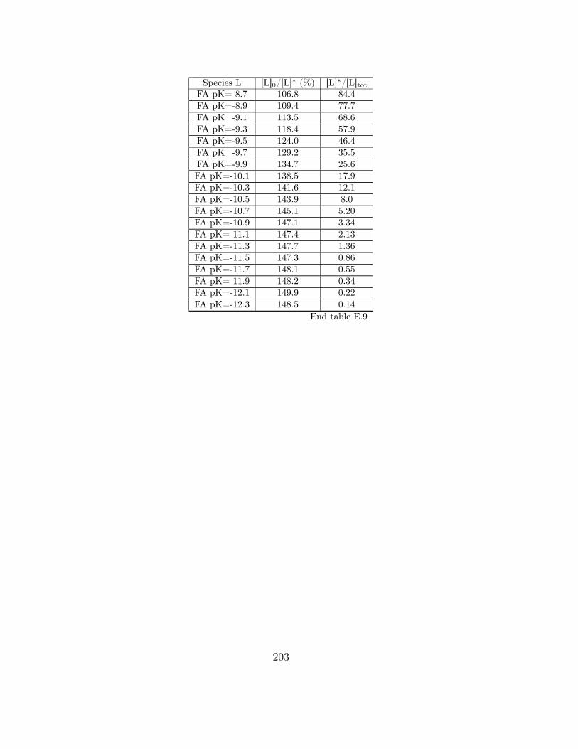
Species L [L]0/[L]∗ (%) [L]∗/[L]totFA pK=-8.7 106.8 84.4FA pK=-8.9 109.4 77.7FA pK=-9.1 113.5 68.6FA pK=-9.3 118.4 57.9FA pK=-9.5 124.0 46.4FA pK=-9.7 129.2 35.5FA pK=-9.9 134.7 25.6FA pK=-10.1 138.5 17.9FA pK=-10.3 141.6 12.1FA pK=-10.5 143.9 8.0FA pK=-10.7 145.1 5.20FA pK=-10.9 147.1 3.34FA pK=-11.1 147.4 2.13FA pK=-11.3 147.7 1.36FA pK=-11.5 147.3 0.86FA pK=-11.7 148.1 0.55FA pK=-11.9 148.2 0.34FA pK=-12.1 149.9 0.22FA pK=-12.3 148.5 0.14

End table E.9

203

Table E.10: Simulation 2d corresponding to [Cu]tot= 10−8M, FAtot=5mg C/L and pH=8.

A) Main general parameters[Cu]tot= 10−8M, pH=8, d = 21.4µm, t = steady-state

Fulvic Acids: FAtot=5mg C/L, LogK∗

0 = 8.54 L/mol, Γ = 0.52, LogK∗ = 13.2

B) Input Parameters to be put in the code

Species X [X]∗ (M) DX (m2s−1) ka (m3mol−1s−1)Cu 5.26 · 10−14 7.14·10−10

OH 1.09 · 10−6 5.27·10−9

FA pK=-10.5 4.25 · 10−8 2.80·10−10

FA pK=-10.7 3.34 · 10−8 2.80·10−10

FA pK=-10.9 2.63 · 10−8 2.80·10−10

FA pK=-11.1 2.06 · 10−8 2.80·10−10

FA pK=-11.3 1.62 · 10−8 2.80·10−10

FA pK=-11.5 1.27 · 10−8 2.80·10−10

FA pK=-11.7 9.86 · 10−9 2.80·10−10

FA pK=-11.9 7.65 · 10−9 2.80·10−10

FA pK=-12.1 5.88 · 10−9 2.80·10−10

FA pK=-12.3 4.47 · 10−9 2.80·10−10

FA pK=-12.5 3.33 · 10−9 2.80·10−10

FA pK=-12.7 2.42 · 10−9 2.80·10−10

FA pK=-12.9 1.70 · 10−9 2.80·10−10

FA pK=-13.1 1.14 · 10−9 2.80·10−10

FA pK=-13.3 7.27 · 10−10 2.80·10−10

FA pK=-13.5 4.40 · 10−10 2.80·10−10

FA pK=-13.7 2.54 · 10−10 2.80·10−10

FA pK=-13.9 1.40 · 10−10 2.80·10−10

FA pK=-14.1 7.50 · 10−11 2.80·10−10

FA pK=-14.3 3.91 · 10−11 2.80·10−10

FA pK=-14.5 2.01 · 10−11 2.80·10−10

FA pK=-14.7 1.02 · 10−11 2.80·10−10

FA pK=-14.9 5.13 · 10−9 2.80·10−10

FA pK=-15.1 2.57 · 10−12 2.80·10−10

FA pK=-15.3 1.28 · 10−12 2.80·10−10

FA pK=-15.5 6.21 · 10−13 2.80·10−10

FA pK=-15.7 3.18 · 10−13 2.80·10−10

FA pK=-15.9 1.58 · 10−13 2.80·10−10

FA pK=-16.1 7.86 · 10−14 2.80·10−10

CuOH 1.05 · 10−13 7.14·10−10 4.98·106

Cu(OH)2 8.88 · 10−13 7.14·10−10 4.15·106

CuFA pK=-10.5 7.08 · 10−11 2.80·10−10 3.31·107

CuFA pK=-10.7 8.82 · 10−11 2.80·10−10 3.31·107

CuFA pK=-10.9 1.10 · 10−10 2.80·10−10 3.31·107

CuFA pK=-11.1 1.37 · 10−10 2.80·10−10 3.31·107

CuFA pK=-11.3 1.70 · 10−10 2.80·10−10 3.31·107

CuFA pK=-11.5 2.11 · 10−10 2.80·10−10 3.31·107

Continued on next page

204

Species X [X]∗ (M) DX (m2s−1) ka (m3mol−1s−1)CuFA pK=-11.7 2.60 · 10−10 2.80·10−10 3.31·107

CuFA pK=-11.9 3.20 · 10−10 2.80·10−10 3.31·107

CuFA pK=-12.1 3.90 · 10−10 2.80·10−10 3.31·107

CuFA pK=-12.3 4.69 · 10−10 2.80·10−10 3.31·107

CuFA pK=-12.5 5.54 · 10−10 2.80·10−10 3.31·107

CuFA pK=-12.7 6.38 · 10−10 2.80·10−10 3.31·107

CuFA pK=-12.9 7.09 · 10−10 2.80·10−10 3.31·107

CuFA pK=-13.1 7.55 · 10−10 2.80·10−10 3.31·107

CuFA pK=-13.3 7.63 · 10−10 2.80·10−10 3.31·107

CuFA pK=-13.5 7.33 · 10−10 2.80·10−10 3.31·107

CuFA pK=-13.7 6.69 · 10−10 2.80·10−10 3.31·107

CuFA pK=-13.9 5.86 · 10−10 2.80·10−10 3.31·107

CuFA pK=-14.1 4.97 · 10−10 2.80·10−10 3.31·107

CuFA pK=-14.3 4.11 · 10−10 2.80·10−10 3.31·107

CuFA pK=-14.5 3.34 · 10−10 2.80·10−10 3.31·107

CuFA pK=-14.7 2.69 · 10−10 2.80·10−10 3.31·107

CuFA pK=-14.9 2.14 · 10−10 2.80·10−10 3.31·107

CuFA pK=-15.1 1.70 · 10−10 2.80·10−10 3.31·107

CuFA pK=-15.3 1.35 · 10−10 2.80·10−10 3.31·107

CuFA pK=-15.5 1.06 · 10−10 2.80·10−10 3.31·107

CuFA pK=-15.7 8.39 · 10−11 2.80·10−10 3.31·107

CuFA pK=-15.9 6.61 · 10−11 2.80·10−10 3.31·107

CuFA pK=-16.1 5.21 · 10−11 2.80·10−10 3.31·107

Results of the simulationJtot=1.32·10−13 mol m−2s−1

∑

JCuXi= 1.25 · 10−13 mol m−2s−1

Jmax = 3.32 · 10−10 mol m−2s−1

Jmin = 1.75 · 10−15 mol m−2s−1

Jlab = 1.40 · 10−10 mol m−2s−1, D = 2.79 · 10−10m2s−1

End table E.10

Table E.11: Complex concentrations and fluxes in the same conditions as table E.10. Detailedresults.

Species ML [ML]0/[ML]∗ (%) [ML]∗/[M]tot (%) J/Jtot (%)CuOH 73.0 <0.01 0.71

Cu(OH)2 85.0 0.01 3.34CuFA pK=-10.5 97.6 0.71 16.6CuFA pK=-10.7 98.3 0.88 14.9CuFA pK=-10.9 99.1 1.10 13.0CuFA pK=-11.1 99.3 1.37 11.0CuFA pK=-11.3 99.4 1.70 9.02CuFA pK=-11.5 99.5 2.11 7.29CuFA pK=-11.7 100.0 2.60 5.80CuFA pK=-11.9 99.7 3.20 4.56

Continued on next page

205

Species ML [ML]0/[ML]∗ (%) [ML]∗/[M]tot (%) J/Jtot (%)CuFA pK=-12.1 99.7 3.90 3.54CuFA pK=-12.3 100.0 4.69 2.70CuFA pK=-12.5 100.0 5.54 2.02CuFA pK=-12.7 100.0 6.38 1.47CuFA pK=-12.9 100.0 7.09 1.03CuFA pK=-13.1 100.0 7.55 0.69CuFA pK=-13.3 100.0 7.63 0.44CuFA pK=-13.5 100.0 7.33 0.27CuFA pK=-13.7 100.0 6.69 0.16CuFA pK=-13.9 100.0 5.86 0.09CuFA pK=-14.1 100.0 4.97 0.05CuFA pK=-14.3 100.0 4.11 0.02CuFA pK=-14.5 100.0 3.34 0.01CuFA pK=-14.7 100.0 2.69 <0.01CuFA pK=-14.9 100.0 2.14 <0.01CuFA pK=-15.1 100.0 1.70 <0.01CuFA pK=-15.3 100.0 1.35 <0.01CuFA pK=-15.5 100.0 1.06 <0.01CuFA pK=-15.7 100.0 0.84 <0.01CuFA pK=-15.9 100.0 0.66 <0.01CuFA pK=-16.1 100.0 0.52 <0.01

End table E.11

Table E.12: Ligand concentrations in the same conditions as table E.10

Species L [L]0/[L]∗ (%) [L]∗/[L]totOH 100.0 100.0

FA pK=-10.5 100.0 100.0FA pK=-10.7 100.0 100.0FA pK=-10.9 100.0 100.0FA pK=-11.1 100.0 100.0FA pK=-11.3 100.0 100.0FA pK=-11.5 100.0 99.2FA pK=-11.7 100.0 98.6FA pK=-11.9 100.0 96.7FA pK=-12.1 100.0 94.5FA pK=-12.3 100.0 91.2FA pK=-12.5 100.0 86.3FA pK=-12.7 100.0 79.9FA pK=-12.9 100.0 71.1FA pK=-13.1 100.0 60.6FA pK=-13.3 100.0 49.1FA pK=-13.5 100.0 37.9FA pK=-13.7 100.0 27.7FA pK=-13.9 100.0 19.4

Continued on next page

206

Species L [L]0/[L]∗ (%) [L]∗/[L]totFA pK=-14.1 100.0 13.2FA pK=-14.3 100.0 8.75FA pK=-14.5 100.0 5.71FA pK=-14.7 100.0 3.68FA pK=-14.9 100.0 2.35FA pK=-15.1 100.0 1.50FA pK=-15.3 100.0 0.95FA pK=-15.5 100.0 0.59FA pK=-15.7 100.0 0.38FA pK=-15.9 100.0 0.24FA pK=-16.1 100.0 0.15

End table E.12

207

Appendix F

List of parameters ofParticles/Aggregates simulations

Table F.1: Results of simulation corresponding to [Cu]tot=10−7M, [L]tot = 1.66 · 10−5M andpH=8.

A) Main general parameters for each simulations[Cu]tot=10−7M, d = 21µm, t = steady-state

Particle Aggregates: rmin = 3nm, rmax = 1µm, K = 9.68 (pH=8), β = 3Fetot = 3 · 10−3g dm−3, Df = 2, [L]tot = 1.66 · 10−5M

B) Input Parameters to be put in the code

Species X [X]∗ (M) DX (m2s−1 ka (m3mol−1s−1) cp BCu 1.27 · 10−12 7.14·10−10

FeOOH1 6.35 · 10−7 2.39·10−13

FeOOH2 6.35 · 10−7 2.99·10−13

FeOOH3 6.35 · 10−7 3.74·10−13

FeOOH4 6.35 · 10−7 4.68·10−13

FeOOH5 6.35 · 10−7 5.85·10−13

FeOOH6 6.35 · 10−7 7.31·10−13

FeOOH7 6.35 · 10−7 9.14·10−13

FeOOH8 6.35 · 10−7 1.14·10−12

FeOOH9 6.35 · 10−7 1.43·10−12

FeOOH10 6.35 · 10−7 1.79·10−12

FeOOH11 6.35 · 10−7 2.24·10−12

FeOOH12 6.35 · 10−7 2.79·10−12

FeOOH13 6.35 · 10−7 3.49·10−12

FeOOH14 6.35 · 10−7 4.37·10−12

FeOOH15 6.35 · 10−7 5.46·10−12

FeOOH16 6.35 · 10−7 6.83·10−12

FeOOH17 6.35 · 10−7 8.54·10−12

FeOOH18 6.35 · 10−7 1.06·10−11

Continued on next page

209

Species X [X]∗ (M) DX (m2s−1 ka (m3mol−1s−1) cp (dm−3) BFeOOH19 6.35 · 10−7 1.34·10−11

FeOOH20 6.35 · 10−7 1.67·10−11

FeOOH21 6.35 · 10−7 2.09·10−11

FeOOH22 6.35 · 10−7 2.61·10−11

FeOOH23 6.35 · 10−7 3.26·10−11

FeOOH24 6.35 · 10−7 4.08·10−11

FeOOH25 6.35 · 10−7 5.10·10−11

FeOOH26 6.35 · 10−7 6.38·10−11

CuFeOOH1 3.85 · 10−9 2.39·10−13 7.26·104 5.74 · 109 3.92 · 103

CuFeOOH2 3.85 · 10−9 2.99·10−13 9.08·104 8.97 · 109 3.13 · 103

CuFeOOH3 3.85 · 10−9 3.74·10−13 1.14·105 1.40 · 1010 2.51 · 103

CuFeOOH4 3.85 · 10−9 4.68·10−13 1.42·105 2.19 · 1010 2.01 · 103

CuFeOOH5 3.85 · 10−9 5.85·10−13 1.77·105 3.43 · 1010 1.60 · 103

CuFeOOH6 3.85 · 10−9 7.31·10−13 2.22·105 5.36 · 1010 1.28 · 103

CuFeOOH7 3.85 · 10−9 9.14·10−13 2.77·105 8.38 · 1010 1.03 · 103

CuFeOOH8 3.85 · 10−9 1.14·10−12 3.47·105 1.31 · 1011 8.20 · 102

CuFeOOH9 3.85 · 10−9 1.43·10−12 4.33·105 2.05 · 1011 6.56 · 102

CuFeOOH10 3.85 · 10−9 1.79·10−12 5.41·105 3.20 · 1011 5.25 · 102

CuFeOOH11 3.85 · 10−9 2.24·10−12 6.77·105 5.00 · 1011 4.20 · 102

CuFeOOH12 3.85 · 10−9 2.79·10−12 8.46·105 7.82 · 1011 3.36 · 102

CuFeOOH13 3.85 · 10−9 3.49·10−12 1.06·106 1.22 · 1012 2.69 · 102

CuFeOOH14 3.85 · 10−9 4.37·10−12 1.32·106 1.91 · 1012 2.15 · 102

CuFeOOH15 3.85 · 10−9 5.46·10−12 1.65·106 2.99 · 1012 1.72 · 102

CuFeOOH16 3.85 · 10−9 6.83·10−12 2.06·106 4.67 · 1012 1.37 · 102

CuFeOOH17 3.85 · 10−9 8.54·10−12 2.57·106 7.31 · 1012 1.10 · 102

CuFeOOH18 3.85 · 10−9 1.07·10−11 3.20·106 1.14 · 1013 8.80 · 101

CuFeOOH19 3.85 · 10−9 1.34·10−11 4.00·106 1.79 · 1013 7.04 · 101

CuFeOOH20 3.85 · 10−9 1.67·10−11 4.98·106 2.79 · 1013 5.63 · 101

CuFeOOH21 3.85 · 10−9 2.09·10−11 6.20·106 4.37 · 1013 4.51 · 101

CuFeOOH22 3.85 · 10−9 2.61·10−11 7.71·106 6.82 · 1013 3.61 · 101

CuFeOOH23 3.85 · 10−9 3.26·10−11 9.57·106 1.07 · 1014 2.89 · 101

CuFeOOH24 3.85 · 10−9 4.08·10−11 1.19·107 1.67 · 1014 2.31 · 101

CuFeOOH25 3.85 · 10−9 5.10·10−11 1.47·107 2.61 · 1014 1.85 · 101

CuFeOOH26 3.85 · 10−9 6.38·10−11 1.81·107 4.08 · 1014 1.48 · 101

Results of the simulationJtot=2.59·10−13 mol m−2s−1

∑

JCuXi= 2.16 · 10−13 mol m−2s−1

Jmax = 3.40 · 10−9 mol m−2s−1

Jmin = 4.30 · 10−14 mol m−2s−1

Jlab = 6.12 · 10−11 mol m−2s−1, D = 1.22 · 10−11m2s−1

End table F.1

210

Table F.2: Complex concentrations and fluxes in the same conditions as table F.1. Detailedresults.

Species ML [ML]0/[ML]∗ (%) [ML]∗/[M]tot (%) J/Jtot (%)CuFeOOH1 99.7 3.85 <0.01CuFeOOH2 99.7 3.85 0.01CuFeOOH3 99.7 3.85 0.02CuFeOOH4 99.7 3.85 0.02CuFeOOH5 99.7 3.85 0.03CuFeOOH6 99.7 3.85 0.05CuFeOOH7 99.7 3.85 0.07CuFeOOH8 99.7 3.85 0.10CuFeOOH9 99.7 3.85 0.15CuFeOOH10 99.7 3.85 0.22CuFeOOH11 99.7 3.85 0.31CuFeOOH12 99.7 3.85 0.45CuFeOOH13 99.7 3.85 0.63CuFeOOH14 99.7 3.85 0.87CuFeOOH15 99.7 3.85 1.19CuFeOOH16 99.5 3.85 1.60CuFeOOH17 99.5 3.85 2.12CuFeOOH18 99.5 3.85 2.75CuFeOOH19 99.5 3.85 3.51CuFeOOH20 99.5 3.85 4.43CuFeOOH21 99.5 3.85 5.54CuFeOOH22 99.5 3.85 6.91CuFeOOH23 99.5 3.85 8.58CuFeOOH24 99.5 3.85 10.6CuFeOOH25 99.5 3.85 13.2CuFeOOH26 99.5 3.85 16.3

End table F.2

Table F.3: Ligand concentrations in the same conditions as table F.1

Species L [L]0/[L]∗ (%) [L]∗/[L]totFeOOH1 100.0 3.83FeOOH1 100.0 3.83FeOOH2 100.0 3.83FeOOH3 100.0 3.83FeOOH4 100.0 3.83FeOOH5 100.0 3.83FeOOH6 100.0 3.83FeOOH7 100.0 3.83FeOOH8 100.0 3.83FeOOH9 100.0 3.83FeOOH10 100.0 3.83

Continued on next page

211

Species L [L]0/[L]∗ (%) [L]∗/[L]totFeOOH11 100.0 3.83FeOOH12 100.0 3.83FeOOH13 100.0 3.83FeOOH14 100.0 3.83FeOOH15 100.0 3.83FeOOH16 100.0 3.83FeOOH17 100.0 3.83FeOOH18 100.0 3.83FeOOH19 100.0 3.83FeOOH20 100.0 3.83FeOOH21 100.0 3.83FeOOH22 100.0 3.83FeOOH23 100.0 3.83FeOOH24 100.0 3.83FeOOH25 100.0 3.83FeOOH26 100.0 3.83

End table F.3

212

Table F.4: Results of simulation corresponding to [Cu]tot=10−7M, [L]tot = 1.66 · 10−7M andpH=8.

A) Main general parameters for each simulations[Cu]tot=10−7M, d = 21µm, t = steady-state

Particle Aggregates: rmin = 3nm, rmax = 1µm, K = 9.68 (pH=8), β = 3Fetot = 3 · 10−5g dm−3, Df = 2, [L]tot = 1.66 · 10−7M

B) Input Parameters to be put in the code

Species X [X]∗ (M) DX (m2s−1) ka (m3mol−1s−1) cp BCu 3.14 · 10−10 7.14·10−10

FeOOH1 2.55 · 10−9 2.39·10−13

FeOOH2 2.55 · 10−9 2.99·10−13

FeOOH3 2.55 · 10−9 3.74·10−13

FeOOH4 2.55 · 10−9 4.68·10−13

FeOOH5 2.55 · 10−9 5.85·10−13

FeOOH6 2.55 · 10−9 7.31·10−13

FeOOH7 2.55 · 10−9 9.14·10−13

FeOOH8 2.55 · 10−9 1.14·10−12

FeOOH9 2.55 · 10−9 1.43·10−12

FeOOH10 2.55 · 10−9 1.79·10−12

FeOOH11 2.55 · 10−9 2.24·10−12

FeOOH12 2.55 · 10−9 2.79·10−12

FeOOH13 2.55 · 10−9 3.49·10−12

FeOOH14 2.55 · 10−9 4.37·10−12

FeOOH15 2.55 · 10−9 5.46·10−12

FeOOH16 2.55 · 10−9 6.83·10−12

FeOOH17 2.55 · 10−9 8.54·10−12

FeOOH18 2.55 · 10−9 1.06·10−11

FeOOH19 2.55 · 10−9 1.34·10−11

FeOOH20 2.55 · 10−9 1.67·10−11

FeOOH21 2.55 · 10−9 2.09·10−11

FeOOH22 2.55 · 10−9 2.61·10−11

FeOOH23 2.55 · 10−9 3.26·10−11

FeOOH24 2.55 · 10−9 4.08·10−11

FeOOH25 2.55 · 10−9 5.10·10−11

FeOOH26 2.55 · 10−9 6.38·10−11

CuFeOOH1 3.83 · 10−9 2.39·10−13 7.08·106 5.74 · 109 3.92 · 101

CuFeOOH2 3.835 · 10−9 2.99·10−13 8.80·106 8.97 · 109 3.13 · 101

CuFeOOH3 3.83 · 10−9 3.74·10−13 1.09·107 1.40 · 1010 2.51 · 101

CuFeOOH4 3.83 · 10−9 4.68·10−13 1.35·107 2.19 · 1010 2.01 · 101

CuFeOOH5 3.83 · 10−9 5.85·10−13 1.67·107 3.43 · 1010 1.60 · 101

CuFeOOH6 3.83 · 10−9 7.31·10−13 2.06·107 5.36 · 1010 1.28 · 101

CuFeOOH7 3.83 · 10−9 9.14·10−13 2.53·107 8.38 · 1010 1.03 · 101

CuFeOOH8 3.83 · 10−9 1.14·10−12 3.09·107 1.31 · 1011 8.20 · 100

CuFeOOH9 3.83 · 10−9 1.43·10−12 3.76·107 2.05 · 1011 6.56 · 100

CuFeOOH10 3.83 · 10−9 1.79·10−12 4.55·107 3.20 · 1011 5.25 · 100

CuFeOOH11 3.83 · 10−9 2.24·10−12 5.47·107 5.00 · 1011 4.20 · 100

Continued on next page

213

Species X [X]∗ (M) DX (m2s−1) ka (m3mol−1s−1) cp (dm−3) BCuFeOOH12 3.83 · 10−9 2.79·10−12 6.52·107 7.82 · 1011 3.36 · 100

CuFeOOH13 3.83 · 10−9 3.49·10−12 7.71·107 1.22 · 1012 2.69 · 100

CuFeOOH14 3.83 · 10−9 4.37·10−12 9.03·107 1.91 · 1012 2.15 · 100

CuFeOOH15 3.83 · 10−9 5.46·10−12 1.05·108 2.99 · 1012 1.72 · 100

CuFeOOH16 3.83 · 10−9 6.83·10−12 1.20·108 4.67 · 1012 1.37 · 100

CuFeOOH17 3.83 · 10−9 8.54·10−12 1.35·108 7.31 · 1012 1.10 · 100

CuFeOOH18 3.83 · 10−9 1.07·10−11 1.51·108 1.14 · 1013 8.80 · 10−1

CuFeOOH19 3.83 · 10−9 1.34·10−11 1.67·108 1.79 · 1013 7.04 · 10−1

CuFeOOH20 3.83 · 10−9 1.67·10−11 1.82·108 2.79 · 1013 5.63 · 10−1

CuFeOOH21 3.83 · 10−9 2.09·10−11 1.96·108 4.37 · 1013 4.51 · 10−1

CuFeOOH22 3.83 · 10−9 2.61·10−11 2.09·108 6.82 · 1013 3.61 · 10−1

CuFeOOH23 3.83 · 10−9 3.26·10−11 2.21·108 1.07 · 1014 2.89 · 10−1

CuFeOOH24 3.83 · 10−9 4.08·10−11 2.31·108 1.67 · 1014 2.31 · 10−1

CuFeOOH25 3.83 · 10−9 5.10·10−11 2.40·108 2.61 · 1014 1.85 · 10−1

CuFeOOH26 3.83 · 10−9 6.38·10−11 2.49·108 4.08 · 1014 1.48 · 10−1

Results of the simulationJtot=1.91·10−11 mol m−2s−1

∑

JCuXi= 8.40e − 12 · 10−12 mol m−2s−1

Jmax = 3.40 · 10−9 mol m−2s−1

Jmin = 1.07 · 10−11 mol m−2s−1

Jlab = 7.20 · 10−11 mol m−2s−1, D = 1.44 · 10−11m2s−1

End table F.4

Table F.5: Complex concentrations and fluxes in the same conditions as table F.4. Detailedresults.

Species ML [ML]0/[ML]∗ (%) [ML]∗/[M]tot (%) J/Jtot (%)CuFeOOH1 73.6 3.83 0.06CuFeOOH2 72.1 3.83 0.08CuFeOOH3 70.8 3.83 0.10CuFeOOH4 70.0 3.83 0.13CuFeOOH5 69.7 3.83 0.17CuFeOOH6 69.7 3.83 0.21CuFeOOH7 69.7 3.83 0.27CuFeOOH8 70.0 3.83 0.33CuFeOOH9 70.5 3.83 0.41CuFeOOH10 70.8 3.83 0.50CuFeOOH11 71.3 3.83 0.61CuFeOOH12 72.1 3.83 0.75CuFeOOH13 72.8 3.83 0.91CuFeOOH14 73.6 3.83 1.11CuFeOOH15 74.7 3.83 1.33CuFeOOH16 75.7 3.83 1.59CuFeOOH17 77.0 3.83 1.88CuFeOOH18 78.6 3.83 2.20

Continued on next page

214

Species ML [ML]0/[ML]∗ (%) [ML]∗/[M]tot (%) J/Jtot (%)CuFeOOH19 80.2 3.83 2.55CuFeOOH20 81.7 3.83 2.93CuFeOOH21 83.6 3.83 3.33CuFeOOH22 85.1 3.83 3.73CuFeOOH23 86.9 3.83 4.13CuFeOOH24 88.5 3.83 4.52CuFeOOH25 90.1 3.83 4.90CuFeOOH26 91.4 3.83 5.25

End table F.5

Table F.6: Ligand concentrations in the same conditions as table F.4

Species L [L]0/[L]∗ (%) [L]∗/[L]totFeOOH1 140.0 1.54FeOOH1 142.4 1.54FeOOH2 144.3 1.54FeOOH3 145.5 1.54FeOOH4 145.9 1.54FeOOH5 145.9 1.54FeOOH6 145.9 1.54FeOOH7 145.5 1.54FeOOH8 144.7 1.54FeOOH9 144.3 1.54FeOOH10 143.1 1.54FeOOH11 142.4 1.54FeOOH12 141.2 1.54FeOOH13 140.0 1.54FeOOH14 138.4 1.54FeOOH15 136.9 1.54FeOOH16 134.9 1.54FeOOH17 132.5 1.54FeOOH18 130.2 1.54FeOOH19 127.8 1.54FeOOH20 125.1 1.54FeOOH21 123.9 1.54FeOOH22 122.7 1.54FeOOH23 120.0 1.54FeOOH24 117.6 1.54FeOOH25 115.3 1.54FeOOH26 112.9 1.54

End table F.6

215

Appendix G

List of parameters of mixturesimulations

Table G.1: Water n 1: Mixtures of Cu + CO3, fulvic acids and particle aggregates. Results ofsimulation corresponding to [Cu]tot=10−8M, [CO3]tot=2·10−3M FAtot=2mg C/L, [L]tot =1.66 · 10−7M and pH=8.

A) Main general parameters for each simulations[Cu]tot=10−8M, d = 20µm, t = steady-state

Natural Inorganic Mixtures: [CO3]tot=2·10−3M, pH=8

Fulvic Acids: FAtot=2mg C/L, LogK∗

0 = 8.54 L/mol, Γ = 0.52, LogK∗ = 12.5Particle Aggregates: rmin = 3nm, rmax = 1µm, K = 9.68 (pH=8), β = 3

Fetot = 3 · 10−5g dm−3, Df = 2, [L]tot = 1.66 · 10−7M

B) Input Parameters to be put in the code

Species X [X]∗ (M) DX (m2s−1) ka (m3mol−1s−1) cp (dm−3) BCu 2.92 · 10−13 7.14·10−10

OH 1.04·10−6 5.27·10−9

CO3 1.02·10−5 9.20·10−10

FA pK=-9.5 5.59 · 10−8 2.80·10−10

FA pK=-9.7 4.40 · 10−8 2.80·10−10

FA pK=-9.9 3.46 · 10−8 2.80·10−10

FA pK=-10.1 2.72 · 10−8 2.80·10−10

FA pK=-10.3 2.14 · 10−8 2.80·10−10

FA pK=-10.5 1.68 · 10−8 2.80·10−10

FA pK=-10.7 1.31 · 10−8 2.80·10−10

FA pK=-10.9 1.02 · 10−8 2.80·10−10

FA pK=-11.1 7.95 · 10−9 2.80·10−10

FA pK=-11.3 6.13 · 10−9 2.80·10−10

FA pK=-11.5 4.67 · 10−9 2.80·10−10

FA pK=-11.7 3.51 · 10−9 2.80·10−10

FA pK=-11.9 2.57 · 10−9 2.80·10−10

FA pK=-12.1 1.82 · 10−9 2.80·10−10

Continued on next page

217

Species X [X]∗ (M) DX (m2s−1) ka (m3mol−1s−1) cp BFA pK=-12.3 1.24 · 10−9 2.80·10−10

FA pK=-12.5 8.02 · 10−10 2.80·10−10

FA pK=-12.7 4.93 · 10−10 2.80·10−10

FA pK=-12.9 2.88 · 10−10 2.80·10−10

FA pK=-13.1 1.61 · 10−10 2.80·10−10

FA pK=-13.3 8.67 · 10−11 2.80·10−10

FA pK=-13.5 4.55 · 10−11 2.80·10−10

FA pK=-13.7 2.34 · 10−11 2.80·10−10

FA pK=-13.9 1.19 · 10−11 2.80·10−10

FA pK=-14.1 6.01 · 10−12 2.80·10−10

FA pK=-14.3 3.01 · 10−12 2.80·10−10

FA pK=-14.5 1.51 · 10−12 2.80·10−10

FA pK=-14.7 7.51 · 10−13 2.80·10−10

FA pK=-14.9 3.74 · 10−13 2.80·10−10

FA pK=-15.1 1.86 · 10−13 2.80·10−10

FA pK=-15.3 9.24 · 10−14 2.80·10−10

FA pK=-15.5 4.59 · 10−14 2.80·10−10

FeOOH1 6.38 · 10−9 2.39·10−13

FeOOH2 6.38 · 10−9 2.99·10−13

FeOOH3 6.38 · 10−9 3.74·10−13

FeOOH4 6.38 · 10−9 4.68·10−13

FeOOH5 6.38 · 10−9 5.85·10−13

FeOOH6 6.38 · 10−9 7.31·10−13

FeOOH7 6.38 · 10−9 9.14·10−13

FeOOH8 6.38 · 10−9 1.14·10−12

FeOOH9 6.38 · 10−9 1.43·10−12

FeOOH10 6.38 · 10−9 1.79·10−12

FeOOH11 6.38 · 10−9 2.24·10−12

FeOOH12 6.38 · 10−9 2.79·10−12

FeOOH13 6.38 · 10−9 3.49·10−12

FeOOH14 6.38 · 10−9 4.37·10−12

FeOOH15 6.38 · 10−9 5.46·10−12

FeOOH16 6.38 · 10−9 6.83·10−12

FeOOH17 6.38 · 10−9 8.54·10−12

FeOOH18 6.38 · 10−9 1.06·10−11

FeOOH19 6.38 · 10−9 1.34·10−11

FeOOH20 6.38 · 10−9 1.67·10−11

FeOOH21 6.38 · 10−9 2.09·10−11

FeOOH22 6.38 · 10−9 2.61·10−11

FeOOH23 6.38 · 10−9 3.26·10−11

FeOOH24 6.38 · 10−9 4.08·10−11

FeOOH25 6.38 · 10−9 5.10·10−11

FeOOH26 6.38 · 10−9 6.38·10−11

CuOH 6.59·10−13 7.14·10−10 4.98·106

Cu(OH)2 5.80·10−12 7.14·10−10 4.15·106

Continued on next page

218

Species X [X]∗ (M) DX (m2s−1) ka (m3mol−1s−1) cp BCu(CO3) 1.25·10−11 7.14·10−10 2.31·107

Cu(CO3)2 2.85·10−13 7.14·10−10 1.93·107

CuFA pK=-9.5 5.17 · 10−11 2.80·10−10 3.31·107

CuFA pK=-9.7 6.44 · 10−11 2.80·10−10 3.31·107

CuFA pK=-9.9 8.03 · 10−11 2.80·10−10 3.31·107

CuFA pK=-10.1 1.00 · 10−10 2.80·10−10 3.31·107

CuFA pK=-10.3 1.24 · 10−10 2.80·10−10 3.31·107

CuFA pK=-10.5 1.55 · 10−10 2.80·10−10 3.31·107

CuFA pK=-10.7 1.92 · 10−10 2.80·10−10 3.31·107

CuFA pK=-10.9 2.38 · 10−10 2.80·10−10 3.31·107

CuFA pK=-11.1 2.92 · 10−10 2.80·10−10 3.31·107

CuFA pK=-11.3 3.57 · 10−10 2.80·10−10 3.31·107

CuFA pK=-11.5 4.32 · 10−10 2.80·10−10 3.31·107

CuFA pK=-11.7 5.13 · 10−10 2.80·10−10 3.31·107

CuFA pK=-11.9 5.96 · 10−10 2.80·10−10 3.31·107

CuFA pK=-12.1 6.69 · 10−10 2.80·10−10 3.31·107

CuFA pK=-12.3 7.21 · 10−10 2.80·10−10 3.31·107

CuFA pK=-12.5 7.40 · 10−10 2.80·10−10 3.31·107

CuFA pK=-12.7 7.21 · 10−10 2.80·10−10 3.31·107

CuFA pK=-12.9 6.68 · 10−10 2.80·10−10 3.31·107

CuFA pK=-13.1 5.91 · 10−10 2.80·10−10 3.31·107

CuFA pK=-13.3 5.05 · 10−10 2.80·10−10 3.31·107

CuFA pK=-13.5 4.20 · 10−10 2.80·10−10 3.31·107

CuFA pK=-13.7 3.43 · 10−10 2.80·10−10 3.31·107

CuFA pK=-13.9 2.77 · 10−10 2.80·10−10 3.31·107

CuFA pK=-14.1 2.21 · 10−10 2.80·10−10 3.31·107

CuFA pK=-14.3 1.76 · 10−10 2.80·10−10 3.31·107

CuFA pK=-14.5 1.39 · 10−10 2.80·10−10 3.31·107

CuFA pK=-14.7 1.10 · 10−10 2.80·10−10 3.31·107

CuFA pK=-14.9 8.67 · 10−11 2.80·10−10 3.31·107

CuFA pK=-15.1 6.84 · 10−11 2.80·10−10 3.31·107

CuFA pK=-15.3 5.39 · 10−11 2.80·10−10 3.31·107

CuFA pK=-15.5 4.24 · 10−11 2.80·10−10 3.31·107

CuFeOOH1 8.91 · 10−12 2.39·10−13 7.08·106 5.74 · 109 3.92 · 101

CuFeOOH2 8.91 · 10−12 2.99·10−13 8.80·106 8.97 · 109 3.13 · 101

CuFeOOH3 8.91 · 10−12 3.74·10−13 1.09·107 1.40 · 1010 2.51 · 101

CuFeOOH4 8.91 · 10−12 4.68·10−13 1.35·107 2.19 · 1010 2.01 · 101

CuFeOOH5 8.91 · 10−12 5.85·10−13 1.67·107 3.43 · 1010 1.60 · 101

CuFeOOH6 8.91 · 10−12 7.31·10−13 2.06·107 5.36 · 1010 1.28 · 101

CuFeOOH7 8.91 · 10−12 9.14·10−13 2.53·107 8.38 · 1010 1.03 · 101

CuFeOOH8 8.91 · 10−12 1.14·10−12 3.09·107 1.31 · 1011 8.20 · 100

CuFeOOH9 8.91 · 10−12 1.43·10−12 3.76·107 2.05 · 1011 6.56 · 100

CuFeOOH10 8.91 · 10−12 1.79·10−12 4.55·107 3.20 · 1011 5.25 · 100

CuFeOOH11 8.91 · 10−12 2.24·10−12 5.47·107 5.00 · 1011 4.20 · 100

CuFeOOH12 8.91 · 10−12 2.79·10−12 6.52·107 7.82 · 1011 3.36 · 100

Continued on next page

219

Species X [X]∗ (M) DX (m2s−1) ka (m3mol−1s−1) cp BCuFeOOH13 8.91 · 10−12 3.49·10−12 7.71·107 1.22 · 1012 2.69 · 100

CuFeOOH14 8.91 · 10−12 4.37·10−12 9.03·107 1.91 · 1012 2.15 · 100

CuFeOOH15 8.91 · 10−12 5.46·10−12 1.05·108 2.99 · 1012 1.72 · 100

CuFeOOH16 8.91 · 10−12 6.83·10−12 1.20·108 4.67 · 1012 1.37 · 100

CuFeOOH17 8.91 · 10−12 8.54·10−12 1.35·108 7.31 · 1012 1.10 · 100

CuFeOOH18 8.91 · 10−12 1.07·10−11 1.51·108 1.14 · 1013 8.80 · 10−1

CuFeOOH19 8.91 · 10−12 1.34·10−11 1.67·108 1.79 · 1013 7.04 · 10−1

CuFeOOH20 8.91 · 10−12 1.67·10−11 1.82·108 2.79 · 1013 5.63 · 10−1

CuFeOOH21 8.91 · 10−12 2.09·10−11 1.96·108 4.37 · 1013 4.51 · 10−1

CuFeOOH22 8.91 · 10−12 2.61·10−11 2.09·108 6.82 · 1013 3.61 · 10−1

CuFeOOH23 8.91 · 10−12 3.26·10−11 2.21·108 1.07 · 1014 2.89 · 10−1

CuFeOOH24 8.91 · 10−12 4.08·10−11 2.31·108 1.67 · 1014 2.31 · 10−1

CuFeOOH25 8.91 · 10−12 5.10·10−11 2.40·108 2.61 · 1014 1.85 · 10−1

CuFeOOH26 8.91 · 10−12 6.38·10−11 2.49·108 4.08 · 1014 1.48 · 10−1

Results of the simulationJtot=1.97·10−12 mol m−2s−1

∑

JCuXi= 1.70 · 10−12 mol m−2s−1 Fulvic Acidd

∑

JCuXi= 2.54 · 10−15 mol m−2s−1 Suspended particles

∑

JCuXi= 2.43 · 10−13 mol m−2s−1 Simple LigandsJmax = 3.56 · 10−10 mol m−2s−1

Jmin = 1.04 · 10−14 mol m−2s−1

Jlab = 1.37 · 10−10 mol m−2s−1, D = 2.75 · 10−10m2s−1

End table G.1

Table G.2: Fulvic Complex concentrations and fluxes in the same conditions as table G.1.Detailed results.

Species ML [ML]0/[ML]∗ (%) [ML]∗/[M]tot (%) J/Jtot (%)CuOH 58.5 0.01 0.40

Cu(OH)2 66.7 0.04 2.65CuCO3 44.0 0.09 9.03

Cu(CO3)2 44.2 <0.01 0.25CuFA pK=-9.5 78.9 0.52 7.69CuFA pK=-9.7 81.8 0.64 8.34CuFA pK=-9.9 84.4 0.80 8.83CuFA pK=-10.1 87.3 1.00 9.05CuFA pK=-10.3 90.3 1.24 8.89CuFA pK=-10.5 92.3 1.55 8.35CuFA pK=-10.7 94.3 1.92 7.48CuFA pK=-10.9 95.8 2.38 6.44CuFA pK=-11.1 97.6 2.92 5.35CuFA pK=-11.3 98.3 3.57 4.31CuFA pK=-11.5 98.8 4.32 3.39CuFA pK=-11.7 99.4 5.13 2.59CuFA pK=-11.9 99.5 5.96 1.92

Continued on next page

220

Species ML [ML]0/[ML]∗ (%) [ML]∗/[M]tot (%) J/Jtot (%)CuFA pK=-12.1 99.7 6.69 1.37CuFA pK=-12.3 99.9 7.21 0.94CuFA pK=-12.5 100.0 7.40 0.61CuFA pK=-12.7 100.0 7.21 0.37CuFA pK=-12.9 100.0 6.68 0.22CuFA pK=-13.1 100.0 5.91 0.12CuFA pK=-13.3 100.0 5.05 0.07CuFA pK=-13.5 100.0 4.20 0.03CuFA pK=-13.7 100.0 3.43 0.02CuFA pK=-13.9 100.0 2.77 0.01CuFA pK=-14.1 100.0 2.21 <0.01CuFA pK=-14.3 100.0 1.76 <0.01CuFA pK=-14.5 100.0 1.39 <0.01CuFA pK=-14.7 100.0 1.10 <0.01CuFA pK=-14.9 100.0 0.87 <0.01CuFA pK=-15.1 100.0 0.68 <0.01CuFA pK=-15.3 100.0 0.54 <0.01CuFA pK=-15.5 100.0 0.42 <0.01

End table G.2

Table G.3: Particle complex concentrations and fluxes in the same conditions as table G.1.Detailed results.

Species ML [ML]0/[ML]∗ (%) [ML]∗/[M]tot (%) J/Jtot (%)CuFeOOH1 99.8 0.09 <0.01CuFeOOH2 99.8 0.09 <0.01CuFeOOH3 99.8 0.09 <0.01CuFeOOH4 99.7 0.09 <0.01CuFeOOH5 99.7 0.09 <0.01CuFeOOH6 99.6 0.09 <0.01CuFeOOH7 99.4 0.09 <0.01CuFeOOH8 99.3 0.09 <0.01CuFeOOH9 99.2 0.09 <0.01CuFeOOH10 99.1 0.09 <0.01CuFeOOH11 99.0 0.09 <0.01CuFeOOH12 98.9 0.01 <0.01CuFeOOH13 98.8 0.01 <0.01CuFeOOH14 98.5 0.01 <0.01CuFeOOH15 98.4 0.01 <0.01CuFeOOH16 98.3 0.01 <0.01CuFeOOH17 98.2 0.01 <0.01CuFeOOH18 98.1 0.01 <0.01CuFeOOH19 98.1 0.01 0.01CuFeOOH20 98.0 0.01 0.01CuFeOOH21 98.0 0.01 0.01

Continued on next page

221

Species ML [ML]0/[ML]∗ (%) [ML]∗/[M]tot (%) J/Jtot (%)CuFeOOH22 98.0 0.01 0.01CuFeOOH23 98.1 0.01 0.01CuFeOOH24 98.1 0.01 0.02CuFeOOH25 98.2 0.01 0.02CuFeOOH26 98.3 0.01 0.02

End table G.3

Table G.4: Ligand concentrations of fulvic acids in the same conditions as table G.1

Species L [L]0/[L]∗ (%) [L]∗/[L]totOH 100.0 100.0CO3 100.0 0.63

FA pK=-9.5 100.0 39.9FA pK=-9.7 100.0 40.0FA pK=-9.9 100.0 39.9FA pK=-10.1 100.0 39.9FA pK=-10.3 100.0 39.9FA pK=-10.5 100.0 39.7FA pK=-10.7 100.0 39.3FA pK=-10.9 100.0 38.9FA pK=-11.1 100.0 38.6FA pK=-11.3 100.0 37.8FA pK=-11.5 100.0 36.5FA pK=-11.7 100.0 35.1FA pK=-11.9 100.0 32.5FA pK=-12.1 100.0 29.3FA pK=-12.3 100.0 25.4FA pK=-12.5 100.0 20.8FA pK=-12.7 100.0 16.3FA pK=-12.9 100.0 12.1FA pK=-13.1 100.0 8.56FA pK=-13.3 100.0 5.86FA pK=-13.5 100.0 3.92FA pK=-13.7 100.0 2.55FA pK=-13.9 100.0 1.65FA pK=-14.1 100.0 1.06FA pK=-14.3 100.0 0.67FA pK=-14.5 100.0 0.43FA pK=-14.7 100.0 0.27FA pK=-14.9 100.0 0.17FA pK=-15.1 100.0 0.11FA pK=-15.3 100.0 0.07FA pK=-15.5 100.0 0.04

End table G.4

222

Table G.5: Ligand concentrations of suspended particles in the same conditions as table G.1

Species L [L]0/[L]∗ (%) [L]∗/[L]totFeOOH1 100.0 3.84FeOOH1 100.0 3.84FeOOH2 100.0 3.84FeOOH3 100.0 3.84FeOOH4 100.0 3.84FeOOH5 100.0 3.84FeOOH6 100.0 3.84FeOOH7 100.0 3.84FeOOH8 100.0 3.84FeOOH9 100.0 3.84FeOOH10 100.0 3.84FeOOH11 100.0 3.84FeOOH12 100.0 3.84FeOOH13 100.0 3.84FeOOH14 100.0 3.84FeOOH15 100.0 3.84FeOOH16 100.0 3.84FeOOH17 100.0 3.84FeOOH18 100.0 3.84FeOOH19 100.0 3.84FeOOH20 100.0 3.84FeOOH21 100.0 3.84FeOOH22 100.0 3.84FeOOH23 100.0 3.84FeOOH24 100.0 3.84FeOOH25 100.0 3.84FeOOH26 100.0 3.84

End table G.5

223

Table G.6: Water n 2: Mixtures of Cu + CO3, fulvic acids and particle aggregates. Resultsof simulation corresponding to [Cu]tot= 3.50−7M, [CO3]tot= 2 · 10−3M FAtot = 2mg C/L,[L]tot = 1.66 · 10−6M and pH=8.

A) Main general parameters for each simulations[Cu]tot= 3.50−7M, d = 20µm, t = steady-state

Natural Inorganic Mixtures: [CO3]tot= 2 · 10−3M, pH=8

Fulvic Acids: FAtot = 2mg C/L, LogK∗

0 = 8.54 L/mol, Γ = 0.52, LogK∗ = 9.5Particle Aggregates: rmin = 3nm, rmax = 1µm, K = 9.68 (pH=8), β = 3

Fetot = 3 · 10−4g dm−3, Df = 2, [L]tot = 1.66 · 10−6M

B) Input Parameters to be put in the code

Species X [X]∗ (M) DX (m2s−1 ka (m3mol−1s−1) cp (dm−3) BCu 3.39 · 10−11 7.14·10−10

OH 1.12·10−6 5.27·10−9

CO3 1.25·10−5 9.20·10−10

FA pK=-7.5 6.13 · 10−7 2.80·10−10

FA pK=-7.7 4.82 · 10−7 2.80·10−10

FA pK=-7.9 3.79 · 10−7 2.80·10−10

FA pK=-8.1 2.98 · 10−7 2.80·10−10

FA pK=-8.3 2.34 · 10−7 2.80·10−10

FA pK=-8.5 1.83 · 10−7 2.80·10−10

FA pK=-8.7 1.43 · 10−7 2.80·10−10

FA pK=-8.9 1.12 · 10−7 2.80·10−10

FA pK=-9.1 8.67 · 10−8 2.80·10−10

FA pK=-9.3 6.66 · 10−8 2.80·10−10

FA pK=-9.5 5.06 · 10−8 2.80·10−10

FA pK=-9.7 3.77 · 10−8 2.80·10−10

FA pK=-9.9 2.73 · 10−8 2.80·10−10

FA pK=-10.1 1.91 · 10−8 2.80·10−10

FA pK=-10.3 1.28 · 10−8 2.80·10−10

FA pK=-10.5 8.15 · 10−9 2.80·10−10

FA pK=-10.7 4.93 · 10−9 2.80·10−10

FA pK=-10.9 2.83 · 10−9 2.80·10−10

FA pK=-11.1 1.56 · 10−9 2.80·10−10

FA pK=-11.3 8.35 · 10−10 2.80·10−10

FA pK=-11.5 4.35 · 10−10 2.80·10−10

FA pK=-11.7 2.23 · 10−10 2.80·10−10

FA pK=-11.9 1.13 · 10−10 2.80·10−10

FA pK=-12.1 5.69 · 10−11 2.80·10−10

FA pK=-12.3 2.85 · 10−11 2.80·10−10

FA pK=-12.5 1.42 · 10−11 2.80·10−10

FA pK=-12.7 7.09 · 10−12 2.80·10−10

FA pK=-12.9 3.53 · 10−12 2.80·10−10

FA pK=-13.1 1.76 · 10−12 2.80·10−10

FA pK=-13.3 8.72 · 10−13 2.80·10−10

FA pK=-13.5 4.33 · 10−13 2.80·10−10

Continued on next page

224

Species X [X]∗ (M) DX (m2s−1 ka (m3mol−1s−1) cp BFeOOH1 5.49 · 10−8 2.39·10−13

FeOOH2 5.49 · 10−8 2.99·10−13

FeOOH3 5.49 · 10−8 3.74·10−13

FeOOH4 5.49 · 10−8 4.68·10−13

FeOOH5 5.49 · 10−8 5.85·10−13

FeOOH6 5.49 · 10−8 7.31·10−13

FeOOH7 5.49 · 10−8 9.14·10−13

FeOOH8 5.49 · 10−8 1.14·10−12

FeOOH9 5.49 · 10−8 1.43·10−12

FeOOH10 5.49 · 10−8 1.79·10−12

FeOOH11 5.49 · 10−8 2.24·10−12

FeOOH12 5.49 · 10−8 2.79·10−12

FeOOH13 5.49 · 10−8 3.49·10−12

FeOOH14 5.49 · 10−8 4.37·10−12

FeOOH15 5.49 · 10−8 5.46·10−12

FeOOH16 5.49 · 10−8 6.83·10−12

FeOOH17 5.49 · 10−8 8.54·10−12

FeOOH18 5.49 · 10−8 1.06·10−11

FeOOH19 5.49 · 10−8 1.34·10−11

FeOOH20 5.49 · 10−8 1.67·10−11

FeOOH21 5.49 · 10−8 2.09·10−11

FeOOH22 5.49 · 10−8 2.61·10−11

FeOOH23 5.49 · 10−8 3.26·10−11

FeOOH24 5.49 · 10−8 4.08·10−11

FeOOH25 5.49 · 10−8 5.10·10−11

FeOOH26 5.49 · 10−8 6.38·10−11

CuOH 6.25·10−11 7.14·10−10 4.98·106

Cu(OH)2 5.13·10−10 7.14·10−10 4.15·106

Cu(CO3) 1.04·10−9 7.14·10−10 2.31·107

Cu(CO3)2 2.90·10−11 7.14·10−10 1.93·107

CuFA pK=-7.5 6.60 · 10−10 2.80·10−10 3.29·107

CuFA pK=-7.7 8.23 · 10−10 2.80·10−10 3.29·107

CuFA pK=-7.9 1.03 · 10−9 2.80·10−10 3.29·107

CuFA pK=-8.1 1.28 · 10−9 2.80·10−10 3.29·107

CuFA pK=-8.3 1.59 · 10−9 2.80·10−10 3.29·107

CuFA pK=-8.5 1.97 · 10−9 2.80·10−10 3.29·107

CuFA pK=-8.7 2.45 · 10−9 2.80·10−10 3.29·107

CuFA pK=-8.9 3.02 · 10−9 2.80·10−10 3.29·107

CuFA pK=-9.1 3.71 · 10−9 2.80·10−10 3.29·107

CuFA pK=-9.3 4.52 · 10−9 2.80·10−10 3.29·107

CuFA pK=-9.5 5.44 · 10−9 2.80·10−10 3.29·107

CuFA pK=-9.7 6.42 · 10−9 2.80·10−10 3.29·107

CuFA pK=-9.9 7.38 · 10−9 2.80·10−10 3.29·107

CuFA pK=-10.1 8.19 · 10−9 2.80·10−10 3.29·107

CuFA pK=-10.3 8.69 · 10−9 2.80·10−10 3.29·107

Continued on next page

225

Species X [X]∗ (M) DX (m2s−1 ka (m3mol−1s−1) cp BCuFA pK=-10.5 8.76 · 10−9 2.80·10−10 3.29·107

CuFA pK=-10.7 8.39 · 10−9 2.80·10−10 3.29·107

CuFA pK=-10.9 7.65 · 10−9 2.80·10−10 3.29·107

CuFA pK=-11.1 6.68 · 10−9 2.80·10−10 3.29·107

CuFA pK=-11.3 5.66 · 10−9 2.80·10−10 3.29·107

CuFA pK=-11.5 4.67 · 10−9 2.80·10−10 3.29·107

CuFA pK=-11.7 3.80 · 10−9 2.80·10−10 3.29·107

CuFA pK=-11.9 3.05 · 10−9 2.80·10−10 3.29·107

CuFA pK=-12.1 2.43 · 10−9 2.80·10−10 3.29·107

CuFA pK=-12.3 1.93 · 10−9 2.80·10−10 3.29·107

CuFA pK=-12.5 1.53 · 10−9 2.80·10−10 3.29·107

CuFA pK=-12.7 1.21 · 10−9 2.80·10−10 3.29·107

CuFA pK=-12.9 9.52 · 10−10 2.80·10−10 3.29·107

CuFA pK=-13.1 7.50 · 10−10 2.80·10−10 3.29·107

CuFA pK=-13.3 5.91 · 10−10 2.80·10−10 3.29·107

CuFA pK=-13.5 4.65 · 10−10 2.80·10−10 3.29·107

Continued on next page

226

Species X [X]∗ (M) DX (m2s−1 ka (m3mol−1s−1) cp BCuFeOOH1 8.95 · 10−9 2.39·10−13 7.18·102 5.74 · 109 3.92 · 102

CuFeOOH2 8.95 · 10−9 2.99·10−13 8.98·102 8.97 · 109 3.13 · 102

CuFeOOH3 8.95 · 10−9 3.74·10−13 1.12·103 1.40 · 1010 2.51 · 102

CuFeOOH4 8.95 · 10−9 4.68·10−13 1.40·103 2.19 · 1010 2.01 · 102

CuFeOOH5 8.95 · 10−9 5.85·10−13 1.75·103 3.43 · 1010 1.60 · 102

CuFeOOH6 8.95 · 10−9 7.31·10−13 2.18·103 5.36 · 1010 1.28 · 102

CuFeOOH7 8.95 · 10−9 9.14·10−13 2.73·103 8.38 · 1010 1.03 · 102

CuFeOOH8 8.95 · 10−9 1.14·10−12 3.40·103 1.31 · 1011 8.20 · 101

CuFeOOH9 8.95 · 10−9 1.43·10−12 4.24·103 2.05 · 1011 6.56 · 101

CuFeOOH10 8.95 · 10−9 1.79·10−12 5.28·103 3.20 · 1011 5.25 · 101

CuFeOOH11 8.95 · 10−9 2.24·10−12 6.57·103 5.00 · 1011 4.20 · 101

CuFeOOH12 8.95 · 10−9 2.79·10−12 8.17·103 7.82 · 1011 3.36 · 101

CuFeOOH13 8.95 · 10−9 3.49·10−12 1.01·104 1.22 · 1012 2.69 · 101

CuFeOOH14 8.95 · 10−9 4.37·10−12 1.26·104 1.91 · 1012 2.15 · 101

CuFeOOH15 8.95 · 10−9 5.46·10−12 1.55·104 2.99 · 1012 1.72 · 101

CuFeOOH16 8.95 · 10−9 6.83·10−12 1.92·104 4.67 · 1012 1.37 · 101

CuFeOOH17 8.95 · 10−9 8.54·10−12 2.36·104 7.31 · 1012 1.10 · 101

CuFeOOH18 8.95 · 10−9 1.07·10−11 2.89·104 1.14 · 1013 8.80 · 100

CuFeOOH19 8.95 · 10−9 1.34·10−11 3.52·104 1.79 · 1013 7.04 · 100

CuFeOOH20 8.95 · 10−9 1.67·10−11 4.27·104 2.79 · 1013 5.63 · 100

CuFeOOH21 8.95 · 10−9 2.09·10−11 5.14·104 4.37 · 1013 4.51 · 100

CuFeOOH22 8.95 · 10−9 2.61·10−11 6.15·104 6.82 · 1013 3.61 · 100

CuFeOOH23 8.95 · 10−9 3.26·10−11 7.29·104 1.07 · 1014 2.89 · 100

CuFeOOH24 8.95 · 10−9 4.08·10−11 8.57·104 1.67 · 1014 2.31 · 100

CuFeOOH25 8.95 · 10−9 5.10·10−11 9.97·104 2.61 · 1014 1.85 · 100

CuFeOOH26 8.95 · 10−9 6.38·10−11 1.15·105 4.08 · 1014 1.48 · 100

Results of the simulationJtot=2.72·10−10 mol m−2s−1

∑

JCuXi= 2.38 · 10−10 mol m−2s−1 for fulvic acid

∑

JCuXi= 1.59 · 10−12 mol m−2s−1 for suspended particles

∑

JCuXi= 2.91 · 10−11 mol m−2s−1 for simple Ligands

Jmax = 1.25 · 10−8 mol m−2s−1

Jmin = 1.21 · 10−12 mol m−2s−1

Jlab = 1.82 · 10−9 mol m−2s−1, D = 1.04 · 10−10m2s−1

End table G.1

Table G.7: Complex concentrations and fluxes of fulvic acids in the same conditions as tableG.6. Detailed results.

Species ML [ML]0/[ML]∗ (%) [ML]∗/[M]tot (%) J/Jtot (%)CuOH 55.7 0.02 0.37

Cu(OH)2 60.7 0.15 2.65CuCO3 45.2 0.30 7.47

Cu(CO3)2 45.2 0.01 0.21CuFA pK=-7.5 50.3 0.19 1.69

Continued on next page

227

Species ML [ML]0/[ML]∗ (%) [ML]∗/[M]tot (%) J/Jtot (%)CuFA pK=-7.7 52.1 0.24 2.03CuFA pK=-7.9 53.9 0.29 2.43CuFA pK=-8.1 55.8 0.37 2.91CuFA pK=-8.3 57.7 0.45 3.46CuFA pK=-8.5 59.6 0.56 4.10CuFA pK=-8.7 61.7 0.70 4.83CuFA pK=-8.9 63.9 0.86 5.61CuFA pK=-9.1 66.4 1.06 6.42CuFA pK=-9.3 69.2 1.29 7.18CuFA pK=-9.5 72.3 1.55 7.76CuFA pK=-9.7 75.8 1.83 8.01CuFA pK=-9.9 79.6 2.11 7.75CuFA pK=-10.1 83.6 2.34 6.93CuFA pK=-10.3 87.4 2.48 5.65CuFA pK=-10.5 90.8 2.50 4.17CuFA pK=-10.7 93.5 2.40 2.81CuFA pK=-10.9 95.6 2.19 1.74CuFA pK=-11.1 97.1 1.91 1.01CuFA pK=-11.3 98.1 1.62 0.56CuFA pK=-11.5 98.8 1.33 0.30CuFA pK=-11.7 99.2 1.09 0.15CuFA pK=-11.9 99.5 0.87 0.08CuFA pK=-12.1 99.7 0.69 0.04CuFA pK=-12.3 99.8 0.55 0.02CuFA pK=-12.5 99.9 0.44 0.01CuFA pK=-12.7 99.9 0.35 0.01CuFA pK=-12.9 99.9 0.27 <0.01CuFA pK=-13.1 100.0 0.21 <0.01CuFA pK=-13.3 100.0 0.17 <0.01CuFA pK=-13.5 100.0 0.13 <0.01

End table G.7

Table G.8: Complex concentrations and fluxes of suspended particles in the same conditionsas table G.6. Detailed results.

Species ML [ML]0/[ML]∗ (%) [ML]∗/[M]tot (%) J/Jtot (%)CuFeOOH1 100.0 2.56 <0.01CuFeOOH2 100.0 2.56 <0.01CuFeOOH3 100.0 2.56 <0.01CuFeOOH4 99.9 2.56 <0.01CuFeOOH5 99.9 2.56 <0.01CuFeOOH6 99.9 2.56 <0.01CuFeOOH7 99.9 2.56 <0.01CuFeOOH8 99.9 2.56 <0.01CuFeOOH9 99.9 2.56 <0.01

Continued on next page

228

Species ML [ML]0/[ML]∗ (%) [ML]∗/[M]tot (%) J/Jtot (%)CuFeOOH10 99.8 2.56 <0.01CuFeOOH11 99.8 2.56 <0.01CuFeOOH12 99.8 2.56 <0.01CuFeOOH13 99.7 2.56 <0.01CuFeOOH14 99.7 2.56 <0.01CuFeOOH15 99.6 2.56 <0.01CuFeOOH16 99.5 2.56 0.01CuFeOOH17 99.4 2.56 0.01CuFeOOH18 99.3 2.56 0.01CuFeOOH19 99.2 2.56 0.02CuFeOOH20 99.1 2.56 0.02CuFeOOH21 99.0 2.56 0.04CuFeOOH22 98.9 2.56 0.05CuFeOOH23 98.8 2.56 0.07CuFeOOH24 98.7 2.56 0.09CuFeOOH25 98.6 2.56 0.12CuFeOOH26 98.6 2.56 0.15

End table G.8

Table G.9: Ligand concentrations of fulvic acids in the same conditions as table G.6

Ligand [L]0/[L]∗ (%) [L]∗/[L]totOH 100.0 100.0CO3 100.0 100.0

FA pK=-7.5 100.1 40.1FA pK=-7.7 100.1 39.8FA pK=-7.9 100.1 39.9FA pK=-8.1 100.2 39.8FA pK=-8.3 100.3 39.7FA pK=-8.5 100.4 39.4FA pK=-8.7 100.7 39.2FA pK=-8.9 101.0 39.0FA pK=-9.1 101.4 38.4FA pK=-9.3 102.1 37.4FA pK=-9.5 103.0 36.1FA pK=-9.7 104.1 34.3FA pK=-9.9 105.5 31.5FA pK=-10.1 107.0 28.0FA pK=-10.3 108.6 23.8FA pK=-10.5 109.9 19.3FA pK=-10.7 111.1 14.8FA pK=-10.9 111.9 10.8FA pK=-11.1 112.6 7.57FA pK=-11.3 113.0 5.15FA pK=-11.5 113.3 3.40

Continued on next page

229

Ligand L [L]0/[L]∗ (%) [L]∗/[L]totFA pK=-11.7 113.5 2.23FA pK=-11.9 113.6 1.43FA pK=-12.1 113.7 0.91FA pK=-12.3 113.7 0.58FA pK=-12.5 113.8 0.37FA pK=-12.7 113.8 0.23FA pK=-12.9 113.8 0.15FA pK=-13.1 113.8 0.09FA pK=-13.3 113.8 0.06FA pK=-13.5 113.8 0.04

End table G.9

Table G.10: Ligand concentrations of suspended particles, in the same conditions as table G.6

Species L [L]0/[L]∗ (%) [L]∗/[L]totFeOOH1 100.0 3.31FeOOH1 100.0 3.31FeOOH2 100.0 3.31FeOOH3 100.0 3.31FeOOH4 100.0 3.31FeOOH5 100.0 3.31FeOOH6 100.0 3.31FeOOH7 100.0 3.31FeOOH8 100.0 3.31FeOOH9 100.0 3.31FeOOH10 100.0 3.31FeOOH11 100.0 3.31FeOOH12 100.0 3.31FeOOH13 100.0 3.31FeOOH14 100.1 3.31FeOOH15 100.1 3.31FeOOH16 100.1 3.31FeOOH17 100.1 3.31FeOOH18 100.1 3.31FeOOH19 100.1 3.31FeOOH20 100.1 3.31FeOOH21 100.2 3.31FeOOH22 100.2 3.31FeOOH23 100.2 3.31FeOOH24 100.2 3.31FeOOH25 100.2 3.31FeOOH26 100.2 3.31

End table G.10

230