A Latent Factor Analysis-Based Approach to Online Sparse

This article has been accepted for inclusion in a future issue of this journal. Content is final as presented, with the exception of pagination.

IEEE TRANSACTIONS ON SYSTEMS, MAN, AND CYBERNETICS: SYSTEMS 1

A Latent Factor Analysis-Based Approach toOnline Sparse Streaming Feature Selection

Di Wu , Member, IEEE, Yi He , Xin Luo , Senior Member, IEEE, and MengChu Zhou , Fellow, IEEE

Abstract—Online streaming feature selection (OSFS) hasattracted extensive attention during the past decades. Currentapproaches commonly assume that the feature space of fixeddata instances dynamically increases without any missing data.However, this assumption does not always hold in many realapplications. Motivated by this observation, this study aimsto implement online feature selection from sparse stream-ing features, i.e., features flow in one by one with missingdata as instance count remains fixed. To do so, this studyproposes a latent-factor-analysis-based online sparse-streaming-feature selection algorithm (LOSSA). Its main idea is to applylatent factor analysis to pre-estimate missing data in sparsestreaming features before conducting feature selection, therebyaddressing the missing data issue effectively and efficiently.Theoretical and empirical studies indicate that LOSSA can sig-nificantly improve the quality of OSFS when missing data areencountered in target instances.

Index Terms—Big data, computational intelligence, latent fac-tor analysis (LFA), missing data, online algorithm, online featureselection, sparse streaming feature, streaming feature.

Manuscript received September 23, 2020; revised March 9, 2021 and May20, 2021; accepted June 30, 2021. This work was supported in part bythe National Natural Science Foundation of China under Grant 61702475,Grant 61772493, Grant 62002337, and Grant 61902370; in part by theNatural Science Foundation of Chongqing, China, under Grant cstc2019jcyj-msxmX0578 and Grant cstc2019jcyjjqX0013; in part by the Chinese Academyof Sciences “Light of West China” Program; in part by the TechnologyInnovation and Application Development Project of Chongqing, China, underGrant cstc2018jszx-cyzdX0041 and Grant cstc2019jscx-fxydX0027; in partby CAAI-Huawei MindSpore Open Fund under Grant CAAIXSJLJJ-2020-004B; and in part by the Pioneer Hundred Talents Program of ChineseAcademy of Sciences. This article was recommended by Associate EditorZ. Yu. (Di Wu and Xin Luo contributed equally to this work.) (Correspondingauthor: Xin Luo.)

Di Wu is with the Chongqing Engineering Research Center of BigData Application for Smart Cities, and the Chongqing Key Laboratory ofBig Data and Intelligent Computing, Chongqing Institute of Green andIntelligent Technology, Chinese Academy of Sciences, Chongqing 400714,China (e-mail: [email protected]).

Yi He is with the Department of Computer Science, Old DominionUniversity, Norfolk, VA 23462 USA (e-mail: [email protected]).

Xin Luo is with the Chongqing Engineering Research Center of BigData Application for Smart Cities, and the Chongqing Key Laboratory ofBig Data and Intelligent Computing, Chongqing Institute of Green andIntelligent Technology, Chinese Academy of Sciences, Chongqing 400714,China, and also with the Department of Big Data Analyses Techniques,Hengrui (Chongqing) Artificial Intelligence Research Center, Cloudwalk,Chongqing 401331, China (e-mail: [email protected]).

MengChu Zhou is with the Helen and John C. Hartmann Department ofElectrical and Computer Engineering, New Jersey Institute of Technology,Newark, NJ 07102 USA, and also with the Institute of Systems Engineeringand Collaborative Laboratory for Intelligent Science and Systems, MacauUniversity of Science and Technology, Macau 999078, China (e-mail:[email protected]).

Color versions of one or more figures in this article are available athttps://doi.org/10.1109/TSMC.2021.3096065.

Digital Object Identifier 10.1109/TSMC.2021.3096065

I. INTRODUCTION

IN THIS era of Information Explosion, people are inun-dated by big data [1]–[3]. For example, Google maintains

more than 20-PB data and Flickr generates more than 3.6-TBdata per day [4]. The global data sum is predicted to growfrom 33 ZB in 2018 to 175 ZB by 2025 [5]. How to effi-ciently filter the valuable information out of mass data for ouruse has become a great challenge [1], [2], [6].

High dimensionality is one of the typical characteristics ofbig data from various areas like healthcare, social media, bioin-formatics, electronic commerce, and online education [7]. Itcauses issues of computation costs and high storage, visu-alization and comprehension difficulties, and performancedegradation on new data [8]. Hence, it is necessary to con-duct feature selection on high-dimensional data [9]–[11]. Assuch, the original data with high dimensionality can be reducedinto a low-dimensional feature space as well as keeping theiressential characteristics to well discriminate each involvedindividual instance [12], [13].

Traditional feature selection approaches mostly assumethat the feature space is predefined and static [14], [15].But in real-world applications, such space usually keepsincreasing dynamically [16], [17], making it impossible toobserve the full feature space in advance [12]. To addressthis issue, many online streaming feature selection (OSFS)approaches are proposed [12], [18]–[25]. For instance, Perkinsand Theiler [18] proposed the Grafting algorithm with a reg-ularized framework. Zhou et al. [19] proposed an Alpha-investing algorithm by using stream-wise regression. Wu et al.,developed a Fast-OSFS algorithm [12] based on onlinerelevance analysis. Besides, other representative algorithmsinclude scalable and accurate online approach (SAOLA) [20]and online selection for features based on adaptive sliding-window (OSFASW) [21].

Despite their efficiency [12], existing OSFS approaches allassume that the input streaming features are complete with-out any missing data. Fig. 1(a) illustrates an example of thisassumption. However, it does not always hold because wecannot completely collect dynamic features in many real appli-cations [28], [29]. For instance, in an intelligent healthcareplatform [26], [27], since the features that describe a patient’ssymptoms may generate from different inspection equipment(respiratory sensors, thermometers, pulse monitors, etc.) andhealthcare service providers (hospitals, insurance companies,labs, etc.), it is impossible to collect all of them. Motivatedby this phenomenon, we formulate such dynamic features

2168-2216 c© 2021 IEEE. Personal use is permitted, but republication/redistribution requires IEEE permission.See https://www.ieee.org/publications/rights/index.html for more information.

Authorized licensed use limited to: CHENGDU BRANCH OF THE NATIONAL SCIENCE LIBRARY CAS. Downloaded on August 06,2021 at 00:49:04 UTC from IEEE Xplore. Restrictions apply.

https://orcid.org/0000-0002-7788-9202

https://orcid.org/0000-0002-5357-6623

https://orcid.org/0000-0002-1348-5305

https://orcid.org/0000-0002-5408-8752


2 IEEE TRANSACTIONS ON SYSTEMS, MAN, AND CYBERNETICS: SYSTEMS

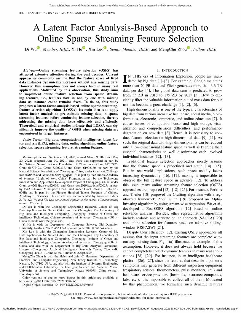
Fig. 1. Example of illustrating the different dynamic features scenarios.Multiple colors denote the observed features, symbols “?” denote the unob-served features (missing data). (a) Streaming features. (b) Sparse streamingfeatures.

as sparse streaming features. As illustrated in Fig. 1(b),sparse streaming features flow in one by one with missingdata while their number of data instances remains fixed. Thus,the problem of Online Sparse Streaming Feature Selection(OS2FS) rises, i.e., how to implement online feature selectionfrom sparse streaming features without information loss?

Sparse data analysis and representation is a vital yet thornyissue in the area of big data analysis and knowledge discov-ery [30]–[37]. To date, a latent factor analysis (LFA)-basedapproach has proven to be highly efficient in addressingit [30]–[37]. For target sparse data, an LFA algorithm modelsthem into a high-dimensional and sparse (HiDS) matrix or ten-sor and builds its low-rank approximation [32], [42]. Note thatall entries of the achieved approximation are available, whichcan be considered as the representation to an HiDS matrix ortensor based on its known data only. Hence, this approxima-tion precisely represents the known data while estimates theunknown ones of an HiDS matrix or tensor [40], [41]. Fromthis point of view, will it be capable of pre-estimating themissing data of sparse streaming features, thereby establish-ing high-quality OS2FS algorithms based on existing OSFSones?

Aiming at answering this question, we for the first timepropose a latent-factor-analysis-based online sparse-streaming-feature selection algorithm (LOSSA). Its main idea is toadopt LFA [30]–[37] to pre-estimate missing data in sparsestreaming features, and then adopt an OSFS algorithm onthe achieved complete features to implement precise featureselection. We attempt to make the following contributions.

1) Formulation of OS2FS Problem: The problem of OSFSis generalized to include online sparse streaming featureselection (OS2FS), which is more frequently encoun-tered in real applications.

2) LOSSA Algorithm: This algorithm is compatible withexisting OSFS algorithms as well as helps them inimplementing high-quality OS2FS without significantmodifications, thereby establishing a new directionin performing OS2FS from the perspective of sparsedata representation learning.

3) Theoretical analysis of the proposed lossa algorithm,including convergence analysis, algorithm design, andtime complexity analysis. From these analyses, theperformance of an LOSSA algorithm is theoreticallyguaranteed.

Empirical studies on 12 benchmark datasets from vari-ous big data-related applications are carefully conducted toevaluate LOSSA’s performance. The results demonstrate thatcompared with existing OSFS algorithms, an LOSSA algo-rithm can effectively improve them to handle the OS2FSproblem.

Section II introduces the preliminaries. Section III presentsLOSSA. Section IV provides the experimental results.Section V discusses related studies. Finally, Section VI con-cludes this article.

II. PRELIMINARIES

A. Notations

Table I summarizes the adopted symbols of this article.

B. Online Feature Selection From Feature Stream

We first define streaming features and OSFS as follows.Definition 1 (Streaming Features [12]): Supposing an

instance set that has M instances and a feature set F thathas N features are given. Let F = {F1, F2, . . . , FN} whereFn = [f1,n, f2,n, . . . , fM,n]T , n ∈ {1, 2, . . . , N}, is a vector thatcorresponds to M instances. Streaming features are encoun-tered when F is presented sequentially. At each time point n,we only observe Fn as N is unknown.

Definition 2 (OSFS [12], [20]): Let On−1 ={F1, F2, . . . , Fn−1} be the observed streaming featuresset till time point n − 1. Let Sn−1 ⊆ On−1 be the selectedstreaming features set at time point n–1. OSFS is taken ata time point n to select a minimum subset Sn from Sn−1∪{Fn}to maximize a resultant model’s performance.

C. Latent Factor Analysis

LFA [30]–[37] originates from decomposition-based matrixmethods [38], [39]. It is widely adopted in many big data-related applications like a recommender system [40], [41].Given a sparse matrix, an LFA model estimates its missingdata by training latent factor matrices based on its knowndata only [32], [42]. We recall its definition [30]–[32], [43].

Definition 3 (LFA): Supposing a sparse matrix YW×Z isgiven, an LFA model is to obtain the rank-d approximationY for Y. It trains two latent factor matrices VZ×d and UW×d

on Y’s known entry set by minimizing the sum errors betweenY and Y, where Y = UVT .

With Definition 3, we see that how to model an objectivefunction to measure the sum errors between Y and Y is verycrucial. Commonly, we adopt Euclidean distance to modelobjective function for LFA [30]–[32], [37], [43]

ε(U, V) = 1

2

∥∥∥��

(

Y − Y)∥∥∥

2

F= 1

2

∥∥�� (Y − UVT)

∥∥

2F (1)

where � denotes the Hadamard product and � is a W × Zbinary index matrix defined as follows:

�w,z ={

1, if yw,z is observed0, otherwise

(2)

where �w,z denotes the entry at the wth row and zth columnof �. To avoid overfitting, L2-norm-based regularization is



WU et al.: LATENT FACTOR ANALYSIS-BASED APPROACH TO ONLINE SPARSE STREAMING FEATURE SELECTION 3

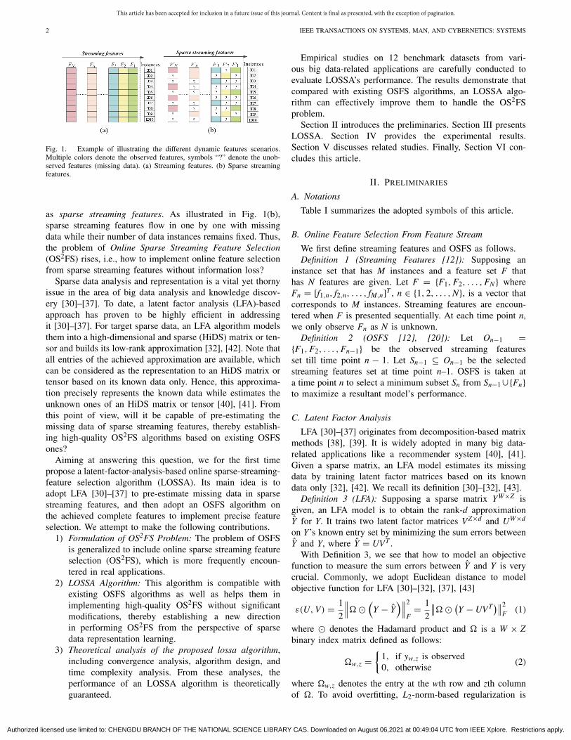
Fig. 2. Flowchart of LOSSA to achieve OS2FS.

TABLE ISYMBOL ANNOTATIONS

incorporated into (1) [30]–[32], [43], resulting in

ε(U, V) = 1

2

∥∥�� (Y − UVT)

∥∥

2F +

λ

2

(

‖U‖2F + ‖V‖2F)

(3)

where λ is the regularization parameter. With an optimizationalgorithm like stochastic gradient descent (SGD) to minimize(3), U and V can be achieved conveniently.

III. PROPOSED ALGORITHM

A. Problem of OS2FS

Definition 4 (Sparse Streaming Features): Corresponding tostreaming features set F = {F1, F2, . . . , FN}, sparse streamingfeatures are encountered when there are some missing data∀Fn = [f1,n, f2,n, . . . , fM,n]T , (n ∈ {1, 2, . . . , N}). Let F′ ={F′1, F′2, . . . , F′N} indicates a set of sparse streaming features.Then the missing data rate αn of F′n is computed by αn =1 − |Kn|/M as Kn be the known entries set of F′n. At eachtime point n, we only observe F′n as N is unknown.

Given F′, let O′n−1 = {F′1, F′2, . . . , F′n−1} be the observedsparse streaming features set till time point n − 1. Let S′n−1be the selected sparse streaming features set at time pointn − 1. Then, we have S′n−1 ⊆ O′n−1. The challenge ofOS2FS is to select a minimum subset S′n from S′n−1

⋃{F′n}to maximize a resultant model’s performance at each timepoint n. Assuming that the concerned model is a classifier withC = [c1, c2, . . . , cM]T being a label vector for M instances,we formulate the problem of OS2FS as

S′n = arg min�

⎧

⎨

⎩|�| : � = arg max

� ⊆S′n−1⋃{F′n}

P(C|�)

⎫

⎬

⎭(4)

where � and � denote a set. Hence, the problem of OS2FSis to select a minimum subset S′n from S′n−1

⋃{F′n} at timepoint n to maximize a classifier’s accuracy on M instanceswith label C = [c1, c2, . . . , cM]T .

B. LOSSA

To make LOSSA as flexible as possible to improve existingOSFS algorithms to handle OS2FS, we design its processingflow, as shown in Fig. 2. LOSSA has two phases. Phase I pre-processes sparse streaming features to complete their missingdata. Phase II performs feature selection from the completedfeatures. Next, a case starting from a time point n is given toelaborate Phase I and Phase II of LOSSA.

1) Phase I: Let BM×BS buffer the arrived sparse streamingfeatures. When it is well filled from time point n to n+BS−1, itconsists of {F′n, F′n+1, . . . , F′n+BS−1}. To address its incomplete

data, we define a completed streaming feature matrix B next.Definition 5 (Completed Streaming Feature Matrix):

Supposing B = {F′n, F′n+1, . . . , F′n+Bs−1} is given. Its com-pleted streaming feature matrix B is B’s rank-d approximation




achieved by training an LFA model on known entries setof B. Features in B denoted by {F′n, F′n+1, . . . , F′n+Bs−1} arecompleted streaming features.

According to Definition 5, to obtain B, it is necessary toapply LFA to B. However, since B contains numerous missingdata, the objective function (3) needs to be reformulated toa single-entry-based form as [30], [32]

∀m ∈ {1, 2, . . . , M} ∀j ∈ {n, n+ 1, . . . , n+ BS − 1}:

ε = 1

2

∑

f ′m,j∈Kj

(

f ′m,j −d∑

k=1

um,kvj,k

)2

+ λ

2

∑

f ′m,j∈Kj

(d∑

k=1

u2m,k +

d∑

k=1

v2j,k

)

(5)

where Kj is the known entries set of F′j , f ′m,j is the mth elementof F′j , uw,k is the kth element of vector uw,., and vj,k is the kthelement of vector vj,.. Note that similar objective functions,e.g., the compound rank-k projections [68], are provided toaddress complete inputs effectively. However, (5) focuses onthe LFs (i.e., projections) related to the known entries of Bonly. With such design, it efficiently and precisely representsbuffered sparse streaming features as shown in Fig. 2.

Consider the instant loss εm,j on a single entry f ′m,j in (5),we have

εm,j = 1

2

(

f ′m,j −d∑

k=1

um,kvj,k

)2

+ λ

2

(d∑

k=1

u2m,k+

d∑

k=1

v2j,k

)

.

(6)

As analyzed in [31], [32], and [44], SGD has the advantageof easy implementation and fast convergence rate. Hence, weadopt SGD to minimize (6)

∀k ∈ {1, 2, . . . , d} :

{

um,k ← um,k − η∂εm,j∂um,k

vj,k ← vj,k − η∂εm,jvqj,k

(7)

where η is the learning rate. By combining (6) and (7), wehave training rules as follows:

On f ′m,j, for k = 1 ∼ d⎧

⎨

⎩

um,k ← um,k + ηvj,k

(

f ′m,j −∑d

k=1 um,kvj,k

)

− ληum,k

vj,k ← vj,k + ηum,k

(

f ′m,j −∑d

k=1 um,kvj,k

)

− ληvj,k.

(8)

With (8), all known entries in B are sequentially adopted totrain U and V in one iteration. As the model converges, U andV are utilized to build B, i.e.,

B = UVT . (9)

Note that the theoretical convergence analysis of Phase I isgiven in the Appendix.

2) Phase II: Let S′n−1 be the completed streaming featuresset in which features are selected from {F′1, F′2, . . . , F′n−1} tilltime point n−1. Then, we present some definitions on F′n andS′n−1 at time point n before introducing Phase II.

Definition 6 (Irrelevant Feature [45]): F′n is an irrelevantfeature to C, if

∀ζ ⊆ S′n−1 s.t. P(

C|ζ, F′n)

= P(C|ζ ). (10)

Definition 7 (Markov Blanket [12]): At time point n − 1,a Markov blanket of C is a subset of S′n−1, represented asMB(C)n−1, MB(C)n−1 ⊆ S′n−1, satisfying

∀ζ ⊆ S′n−1 −MB(C)n−1

s.t. P(C|MB(C)n−1, ζ ) = P(C|MB(C)n−1) (11)

where S′n−1−MB(C)n−1 denotes the subset of S′n−1 excludingMB(C)n−1.

Definition 8 (Redundant Completed Streaming Features):At time point n, if F′n is not an irrelevant feature to C, theredundant completed streaming features to C satisfy

∀R ∈ MB(C)n−1

⋃{

F′n}

, ∃ζ ⊆ MB(C)n−1

⋃{

F′n}

− {R}s.t. P(C|R, ζ ) = P(C|ζ ) (12)

where R indicates a redundant completed streaming featureto C and MB(C)n−1

⋃{F′n} − {R} indicates the subset ofMB(C)n−1

⋃{F′n} excluding {R}.Although existing OSFS approaches work differently, their

processing flows are similar and can be concluded into twomain parts [12], [20]–[23]: 1) online relevance analysis and2) online redundancy analysis. Next, we explain how to con-duct online feature selection on B (obtained from Phase I)in Phase II following Definitions 6–8 with a small examplestarting from time point n to n+ BS − 1.

1) Initialization: Initializing a cache set CS = S′n−1, a labelvector C, and a Markov blanket MB(C)n−1 ⊆ CS thatsatisfies ∀ ⊆ CS − MB(C)n−1 s.t. P(C|MB(C)n−1, ) =P(C|MB(C)n−1).

2) Online Relevance Analysis: ∀i ∈ {0, 1, . . . , BS − 1}, afeature F′n+i in B is sequentially analyzed with C fol-lowing Definition 6. If a feature is irrelevant to C, i.e.,∀ ⊆ CS s.t. P(C|ζ, F′n+i) = P(C|ζ ), it is discarded;otherwise, it is added to CS.

3) Online Redundancy Analysis: Each feature Q in CSis sequentially identified with C following Definition8. If a feature is redundant to C, i.e., if ∀R ⊆MB(C)n−1

⋃{Q}, ∃ ⊆ MB(C)n−1⋃{Q} − {R} s.t.

P(C|ζR, F′n+i) = P(C|ζ ), it is removed from CS.After the above three steps, the remaining features in CS

are the best-selected and completed streaming features at thecurrent time point n + BS − 1. Please note that Phase II ofLOSSA focuses on the task of streaming feature selectionon the completed streaming feature matrix B, which does notinvolve convergence issues as discussed in [12] and [18]–[25].

C. Algorithm Design and Time Complexity Analysis

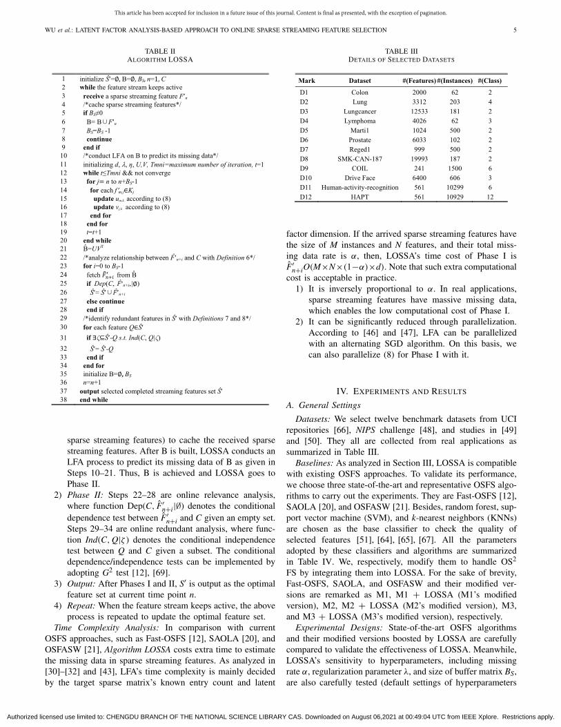
Algorithm Design: Based on the above analyses, we designAlgorithm LOSSA to handle the problem of OS2FS. Its pseudocode is given in Table II, where Phase I consists of steps 4–21and Phase II consists of steps 22–37.

1) Phase I: Steps 4–9 adopt a buffer matrix B (whosecolumn count BS is far less than the total number of




TABLE IIALGORITHM LOSSA

sparse streaming features) to cache the received sparsestreaming features. After B is built, LOSSA conducts anLFA process to predict its missing data of B as given inSteps 10–21. Thus, B is achieved and LOSSA goes toPhase II.

2) Phase II: Steps 22–28 are online relevance analysis,where function Dep(C, F′n+i|∅) denotes the conditionaldependence test between F′n+i and C given an empty set.Steps 29–34 are online redundant analysis, where func-tion Ind(C, Q|ζ ) denotes the conditional independencetest between Q and C given a subset. The conditionaldependence/independence tests can be implemented byadopting G2 test [12], [69].

3) Output: After Phases I and II, S′ is output as the optimalfeature set at current time point n.

4) Repeat: When the feature stream keeps active, the aboveprocess is repeated to update the optimal feature set.

Time Complexity Analysis: In comparison with currentOSFS approaches, such as Fast-OSFS [12], SAOLA [20], andOSFASW [21], Algorithm LOSSA costs extra time to estimatethe missing data in sparse streaming features. As analyzed in[30]–[32] and [43], LFA’s time complexity is mainly decidedby the target sparse matrix’s known entry count and latent

TABLE IIIDETAILS OF SELECTED DATASETS

factor dimension. If the arrived sparse streaming features havethe size of M instances and N features, and their total miss-ing data rate is α, then, LOSSA’s time cost of Phase I isF′n+iO(M×N×(1−α)×d). Note that such extra computationalcost is acceptable in practice.

1) It is inversely proportional to α. In real applications,sparse streaming features have massive missing data,which enables the low computational cost of Phase I.

2) It can be significantly reduced through parallelization.According to [46] and [47], LFA can be parallelizedwith an alternating SGD algorithm. On this basis, wecan also parallelize (8) for Phase I with it.

IV. EXPERIMENTS AND RESULTS

A. General Settings

Datasets: We select twelve benchmark datasets from UCIrepositories [66], NIPS challenge [48], and studies in [49]and [50]. They all are collected from real applications assummarized in Table III.

Baselines: As analyzed in Section III, LOSSA is compatiblewith existing OSFS approaches. To validate its performance,we choose three state-of-the-art and representative OSFS algo-rithms to carry out the experiments. They are Fast-OSFS [12],SAOLA [20], and OSFASW [21]. Besides, random forest, sup-port vector machine (SVM), and k-nearest neighbors (KNNs)are chosen as the base classifier to check the quality ofselected features [51], [64], [65], [67]. All the parametersadopted by these classifiers and algorithms are summarizedin Table IV. We, respectively, modify them to handle OS2

FS by integrating them into LOSSA. For the sake of brevity,Fast-OSFS, SAOLA, and OSFASW and their modified ver-sions are remarked as M1, M1 + LOSSA (M1’s modifiedversion), M2, M2 + LOSSA (M2’s modified version), M3,and M3 + LOSSA (M3’s modified version), respectively.

Experimental Designs: State-of-the-art OSFS algorithmsand their modified versions boosted by LOSSA are carefullycompared to validate the effectiveness of LOSSA. Meanwhile,LOSSA’s sensitivity to hyperparameters, including missingrate α, regularization parameter λ, and size of buffer matrix BS,are also carefully tested (default settings of hyperparameters




TABLE IVALL THE PARAMETERS USED IN THE EXPERIMENTS

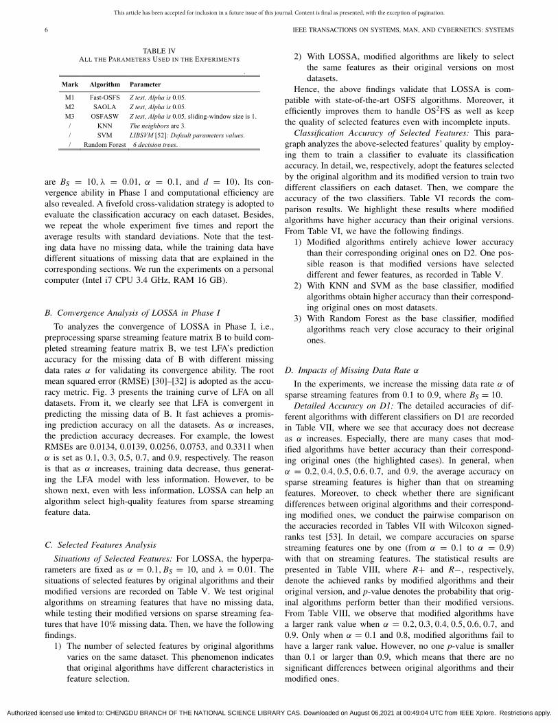
are BS = 10, λ = 0.01, α = 0.1, and d = 10). Its con-vergence ability in Phase I and computational efficiency arealso revealed. A fivefold cross-validation strategy is adopted toevaluate the classification accuracy on each dataset. Besides,we repeat the whole experiment five times and report theaverage results with standard deviations. Note that the test-ing data have no missing data, while the training data havedifferent situations of missing data that are explained in thecorresponding sections. We run the experiments on a personalcomputer (Intel i7 CPU 3.4 GHz, RAM 16 GB).

B. Convergence Analysis of LOSSA in Phase I

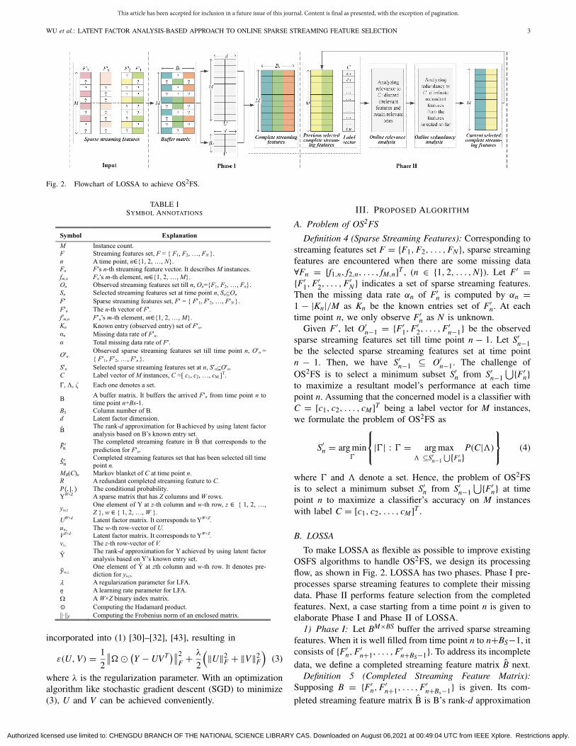
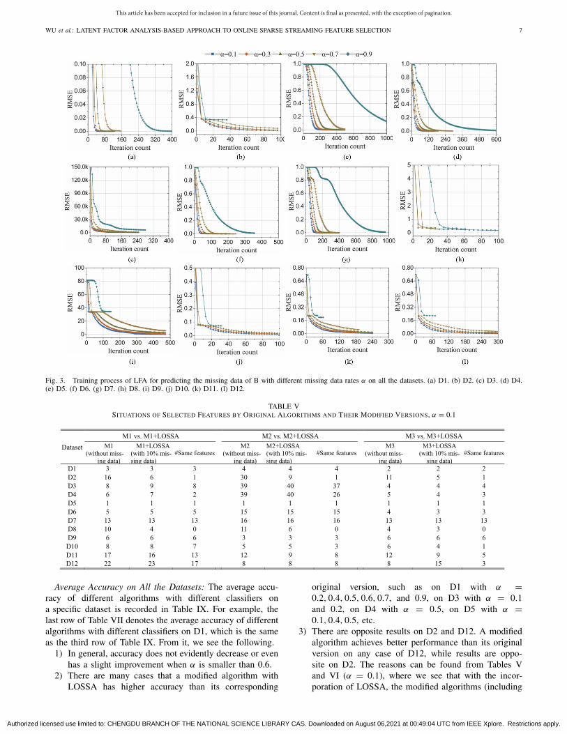
To analyzes the convergence of LOSSA in Phase I, i.e.,preprocessing sparse streaming feature matrix B to build com-pleted streaming feature matrix B, we test LFA’s predictionaccuracy for the missing data of B with different missingdata rates α for validating its convergence ability. The rootmean squared error (RMSE) [30]–[32] is adopted as the accu-racy metric. Fig. 3 presents the training curve of LFA on alldatasets. From it, we clearly see that LFA is convergent inpredicting the missing data of B. It fast achieves a promis-ing prediction accuracy on all the datasets. As α increases,the prediction accuracy decreases. For example, the lowestRMSEs are 0.0134, 0.0139, 0.0256, 0.0753, and 0.3311 whenα is set as 0.1, 0.3, 0.5, 0.7, and 0.9, respectively. The reasonis that as α increases, training data decrease, thus generat-ing the LFA model with less information. However, to beshown next, even with less information, LOSSA can help analgorithm select high-quality features from sparse streamingfeature data.

C. Selected Features Analysis

Situations of Selected Features: For LOSSA, the hyperpa-rameters are fixed as α = 0.1, BS = 10, and λ = 0.01. Thesituations of selected features by original algorithms and theirmodified versions are recorded on Table V. We test originalalgorithms on streaming features that have no missing data,while testing their modified versions on sparse streaming fea-tures that have 10% missing data. Then, we have the followingfindings.

1) The number of selected features by original algorithmsvaries on the same dataset. This phenomenon indicatesthat original algorithms have different characteristics infeature selection.

2) With LOSSA, modified algorithms are likely to selectthe same features as their original versions on mostdatasets.

Hence, the above findings validate that LOSSA is com-patible with state-of-the-art OSFS algorithms. Moreover, itefficiently improves them to handle OS2FS as well as keepthe quality of selected features even with incomplete inputs.

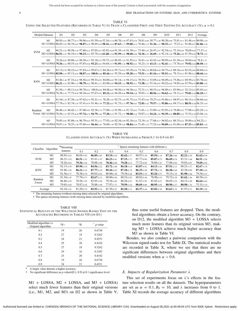
Classification Accuracy of Selected Features: This para-graph analyzes the above-selected features’ quality by employ-ing them to train a classifier to evaluate its classificationaccuracy. In detail, we, respectively, adopt the features selectedby the original algorithm and its modified version to train twodifferent classifiers on each dataset. Then, we compare theaccuracy of the two classifiers. Table VI records the com-parison results. We highlight these results where modifiedalgorithms have higher accuracy than their original versions.From Table VI, we have the following findings.

1) Modified algorithms entirely achieve lower accuracythan their corresponding original ones on D2. One pos-sible reason is that modified versions have selecteddifferent and fewer features, as recorded in Table V.

2) With KNN and SVM as the base classifier, modifiedalgorithms obtain higher accuracy than their correspond-ing original ones on most datasets.

3) With Random Forest as the base classifier, modifiedalgorithms reach very close accuracy to their originalones.

D. Impacts of Missing Data Rate α

In the experiments, we increase the missing data rate α ofsparse streaming features from 0.1 to 0.9, where BS = 10.

Detailed Accuracy on D1: The detailed accuracies of dif-ferent algorithms with different classifiers on D1 are recordedin Table VII, where we see that accuracy does not decreaseas α increases. Especially, there are many cases that mod-ified algorithms have better accuracy than their correspond-ing original ones (the highlighted cases). In general, whenα = 0.2, 0.4, 0.5, 0.6, 0.7, and 0.9, the average accuracy onsparse streaming features is higher than that on streamingfeatures. Moreover, to check whether there are significantdifferences between original algorithms and their correspond-ing modified ones, we conduct the pairwise comparison onthe accuracies recorded in Tables VII with Wilcoxon signed-ranks test [53]. In detail, we compare accuracies on sparsestreaming features one by one (from α = 0.1 to α = 0.9)with that on streaming features. The statistical results arepresented in Table VIII, where R+ and R−, respectively,denote the achieved ranks by modified algorithms and theiroriginal version, and p-value denotes the probability that orig-inal algorithms perform better than their modified versions.From Table VIII, we observe that modified algorithms havea larger rank value when α = 0.2, 0.3, 0.4, 0.5, 0.6, 0.7, and0.9. Only when α = 0.1 and 0.8, modified algorithms fail tohave a larger rank value. However, no one p-value is smallerthan 0.1 or larger than 0.9, which means that there are nosignificant differences between original algorithms and theirmodified ones.




Fig. 3. Training process of LFA for predicting the missing data of B with different missing data rates α on all the datasets. (a) D1. (b) D2. (c) D3. (d) D4.(e) D5. (f) D6. (g) D7. (h) D8. (i) D9. (j) D10. (k) D11. (l) D12.

TABLE VSITUATIONS OF SELECTED FEATURES BY ORIGINAL ALGORITHMS AND THEIR MODIFIED VERSIONS, α = 0.1

Average Accuracy on All the Datasets: The average accu-racy of different algorithms with different classifiers ona specific dataset is recorded in Table IX. For example, thelast row of Table VII denotes the average accuracy of differentalgorithms with different classifiers on D1, which is the sameas the third row of Table IX. From it, we see the following.

1) In general, accuracy does not evidently decrease or evenhas a slight improvement when α is smaller than 0.6.

2) There are many cases that a modified algorithm withLOSSA has higher accuracy than its corresponding

original version, such as on D1 with α =0.2, 0.4, 0.5, 0.6, 0.7, and 0.9, on D3 with α = 0.1and 0.2, on D4 with α = 0.5, on D5 with α =0.1, 0.4, 0.5, etc.

3) There are opposite results on D2 and D12. A modifiedalgorithm achieves better performance than its originalversion on any case of D12, while results are oppo-site on D2. The reasons can be found from Tables Vand VI (α = 0.1), where we see that with the incor-poration of LOSSA, the modified algorithms (including




TABLE VIUSING THE SELECTED FEATURES (RECORDED IN TABLE V) TO TRAIN A CLASSIFIER FIRST AND THEN TESTING ITS ACCURACY (%), α = 0.1

TABLE VIICLASSIFICATION ACCURACY (%) WHEN INCREASING α FROM 0.1 TO 0.9 ON D1

TABLE VIIISTATISTICAL RESULTS OF THE WILCOXON SIGNED-RANKS TEST ON THE

ACCURACIES RECORDED IN TABLES VII (ON D1)

M1 + LOSSA, M2 + LOSSA, and M3 + LOSSA)select much fewer features than their original versions(i.e., M1, M2, and M3) on D2 as shown in Table V,

thus some useful features are dropped. Then, the modi-fied algorithms obtain a lower accuracy. On the contrary,on D12, the modified algorithm M3 + LOSSA selectsmuch more features than its original version M3, mak-ing M3 + LOSSA achieve much higher accuracy thanM3 as shown in Table VI.

Besides, we also conduct a pairwise comparison with theWilcoxon signed-ranks test for Table IX. The statistical resultsare recorded in Table X, where we see that there are nosignificant differences between original algorithms and theirmodified versions when α < 0.6.

E. Impacts of Regularization Parameter λ

This set of experiments focus on λ’s effects in the fea-ture selection results on all the datasets. The hyperparametersare set as α = 0.1, BS = 10, and λ increases from 0 to 1.Table XI records the average accuracy of different algorithms




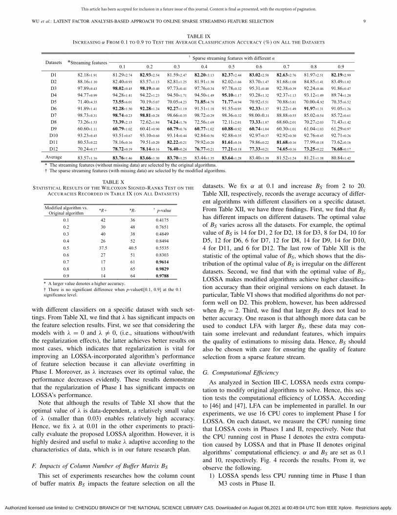
TABLE IXINCREASING α FROM 0.1 TO 0.9 TO TEST THE AVERAGE CLASSIFICATION ACCURACY (%) ON ALL THE DATASETS

TABLE XSTATISTICAL RESULTS OF THE WILCOXON SIGNED-RANKS TEST ON THE

ACCURACIES RECORDED IN TABLE IX (ON ALL DATASETS)

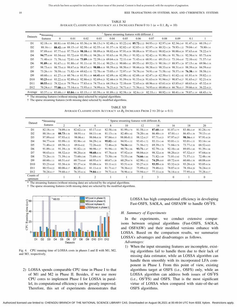
with different classifiers on a specific dataset with such set-tings. From Table XI, we find that λ has significant impacts onthe feature selection results. First, we see that considering themodels with λ = 0 and λ �= 0, (i.e., situations without/withthe regularization effects), the latter achieves better results onmost cases, which indicates that regularization is vital forimproving an LOSSA-incorporated algorithm’s performanceof feature selection because it can alleviate overfitting inPhase I. Moreover, as λ increases over its optimal value, theperformance decreases evidently. These results demonstratethat the regularization of Phase I has significant impacts onLOSSA’s performance.

Note that although the results of Table XI show that theoptimal value of λ is data-dependent, a relatively small valueof λ (smaller than 0.03) enables relatively high accuracy.Hence, we fix λ at 0.01 in the other experiments to practi-cally evaluate the proposed LOSSA algorithm. However, it ishighly desired and useful to make λ adaptive according to thecharacteristics of data, which is in our future research plan.

F. Impacts of Column Number of Buffer Matrix BS

This set of experiments researches how the column countof buffer matrix BS impacts the feature selection on all the

datasets. We fix α at 0.1 and increase BS from 2 to 20.Table XII, respectively, records the average accuracy of differ-ent algorithms with different classifiers on a specific dataset.From Table XII, we have three findings. First, we find that BS

has different impacts on different datasets. The optimal valueof BS varies across all the datasets. For example, the optimalvalue of BS is 14 for D1, 2 for D2, 18 for D3, 8 for D4, 10 forD5, 12 for D6, 6 for D7, 12 for D8, 14 for D9, 14 for D10,4 for D11, and 6 for D12. The last row of Table XII is thestatistic of the optimal value of BS, which shows that the dis-tribution of the optimal value of BS is irregular on the differentdatasets. Second, we find that with the optimal value of BS,LOSSA makes modified algorithms achieve higher classifica-tion accuracy than their original versions on each dataset. Inparticular, Table VI shows that modified algorithms do not per-form well on D2. This problem, however, has been addressedwhen BS = 2. Third, we find that larger BS does not lead tobetter accuracy. One reason is that although more data can beused to conduct LFA with larger BS, these data may con-tain some irrelevant and redundant features, which impairsthe quality of estimations to missing data. Hence, BS shouldalso be chosen with care for ensuring the quality of featureselection from a sparse feature stream.

G. Computational Efficiency

As analyzed in Section III-C, LOSSA needs extra compu-tation to modify original algorithms to solve. Hence, this sec-tion tests the computational efficiency of LOSSA. Accordingto [46] and [47], LFA can be implemented in parallel. In ourexperiments, we use 16 CPU cores to implement Phase I forLOSSA. On each dataset, we measure the CPU running timethat LOSSA costs in Phases I and II, respectively. Note thatthe CPU running cost in Phase I denotes the extra computa-tion caused by LOSSA and that in Phase II denotes originalalgorithms’ computational efficiency. α and BS are set as 0.1and 10, respectively. Fig. 4 records the results. From it, weobserve the following.

1) LOSSA spends less CPU running time in Phase I thanM3 costs in Phase II.




TABLE XIAVERAGE CLASSIFICATION ACCURACY AS λ INCREASES FROM 0 TO 1 (α = 0.1, BS = 10)

TABLE XIIAVERAGE CLASSIFICATION ACCURACY AS BS INCREASES FROM 2 TO 20 (α = 0.1)

Fig. 4. CPU running time of LOSSA costs in phases I and II with M1, M2,and M3, respectively.

2) LOSSA spends comparable CPU time in Phase I to thatof M1 and M2 in Phase II. Besides, if we use moreCPU cores to implement Phase I for LOSSA in paral-lel, its computational efficiency can be greatly improved.Therefore, this set of experiments demonstrates that

LOSSA has high computational efficiency in developingFast-OSFS, SAOLA, and OSFASW to handle OS2FS.

H. Summary of Experiments

In the experiments, we conduct extensive compar-isons between original algorithms (Fast-OSFS, SAOLA,and OSFASW) and their modified versions enhance withLOSSA. Based on the comparison results, we summarizeLOSSA’s advantages and disadvantages as follows.

Advantages:1) When the input streaming features are incomplete, exist-

ing algorithms fail to handle them due to their lack ofmissing data estimator, while an LOSSA algorithm canhandle them smoothly with its incorporated LFA com-ponent in Phase I. From this point of view, existingalgorithms target at OSFS (i.e., OSFS) only, while anLOSSA algorithm can address both issues of OS2FS(i.e., OS2FS) and OSFS. That is the most significantvirtue of LOSSA when compared with state-of-the-artOSFS algorithms.




2) LOSSA is compatible with existing OSFS algorithmswithout changing their mechanisms or working schemes.Moreover, it helps them in implementing high-qualityfeature selection in the case of OS2FS. Especially, whenthe missing data rate α is smaller than 0.6, it caneffectively improve existing OSFS algorithms to handleOS2FS with high accuracy.

Disadvantages:1) It has to tune parameters (λ and BS) to achieve

the best performance. Currently, this issue can beaddressed via conducting pretuning process on warming-up datasets. We plan to make this parameter self-adaptive as future work.

2) It needs extra computation to complete missingdata of sparse streaming features in Phase I.However, such extra computational cost is acceptablein practice and can be significantly reduced throughparallelization [46], [47].

V. RELATED WORK

The proposed LOSSA is closely related to LFA on sparsedata. In it, LFA is adopted to complete the missing data ofsparse streaming features before conducting feature selectionowing to its high efficiency of storage and computation, aswell as high representation learning ability on sparse data [60].Besides LFA, other techniques like multiple imputations,expectation-maximization (EM), regression imputation, andmatrix completion, can also address such a problem [60]–[63].However, multiple imputations, EM, and regression imputa-tions do not perform well when the missing rate is high [60].Candès and Recht [61] and Keshavan et al. [62], respec-tively, proposed a matrix completion approach to address sucha problem with nice accuracy. However, they are expensive inboth computation and storage [63].

Meanwhile, the online feature selection problem can be fur-ther categorized into two branches [7], i.e., online featureselection from streaming data (OFSSD) and OSFS. OFSSDassumes that the feature size remains fixed while data instancesincrease over time [25], [56]–[59], while OSFS assumes thatthe data instance count is fixed and the feature dimensionincreases with time [12], [18]–[23]. In this article, we focuson the latter, i.e., OSFS.

To date, great efforts have been paid to handle OSFSissue [12], [18]–[25]. Perkins and Theiler [18] proposed theGrafting algorithm based on a regularized framework. SinceGrafting needs to carefully tune its regularization parameterbefore determining which feature is most likely to be selected,it is ineffective to process the streaming features whose sizeis unknown [12]. Zhou et al. [19] an Alpha-investing algo-rithm by using stream-wise regression. Dhillon et al. [24]extended this algorithm to handle the problem of multiplefeature classes. Although they can handle infinite stream-ing features, they are limited by their dependence on priorknowledge [23].

Wu et al. proposed an OSFS framework based on two parts,i.e., online relevance analysis and online redundancy analy-sis. Then, they develop the Fast-OSFS algorithm [12]. Based

on this framework, several algorithms have been proposedrecently, including an OGFS algorithm [25] that can handlegroup streaming features with group structure information asprior knowledge, an SAOLA algorithm [20] that is designedfor extremely high dimensional feature selection, an OSFASWalgorithm [21] that has high prediction accuracy and reducesthe selected features number by using self-adaptive sliding-window sampling, an OFS-Density algorithm [22] that doesnot need the domain information by using adaptive densityneighborhood relation, an OFS-A3M algorithm [23] that doesnot also need the domain information and specify any param-eter in advance by utilizing an adaptive neighborhood roughset, ROSFSMI algorithm [76] that employs mutual informationin a streaming manner to evaluate the relevancy and redun-dancy of features, SFS-FI [77] algorithm that can selectstreaming features to interact with each other, and OGSFS-FI algorithm [78] that considers feature interaction within andbetween the streaming groups during feature selection.

The above algorithms are sophisticated OSFS algorithmswith high efficiency. However, they can only process stream-ing features without missing data, while streaming features inmost real-world applications have missing data. The proposedLOSSA, in comparison, makes significant progress in address-ing the real-world feature selection with missing data. It fitsindustrial needs more appropriately than the prior methodswhen dealing with streaming features with missing data.

VI. CONCLUSION

This article proposes an LOSSA to handle OS2FS problemwell. Its main idea is to adopt LFA to pre-estimate the miss-ing data of sparse streaming features before selection, therebyimplementing effective and efficient feature selection. It iscompatible with the current OSFS approaches. In particu-lar, three state-of-the-art OSFS algorithms are enhanced withLOSSA to conduct the experiments on twelve benchmarkclassification datasets. The experimental results well validateLOSSA’s capability of effectively boosting an OSFS algorithmto address the issue of OS2FS precisely.

Note that some hyperparameters of LOSSA, including thesize of a buffer matrix and regularization coefficient, requiremanual tuning that is time-consuming and tedious. It is vitalto make them self-adaptive through evolutionary computationalgorithms [54], [55] or other feasible frameworks to improveLOSSA’s practicability. Meanwhile, representation learning isanother promising way to process high-dimensional data, likeneural networks-based one [74] and Bayesian-based one [75].It is also highly interesting to extend LOSSA to be compatiblewith representation learning approaches and gain more appli-cations [79], [80]. We plan to address these challenging issuesin our future work.

APPENDIX

A. Theoretical Convergence Analysis of Phase I

This section theoretically analyzes the convergence ofPhase I in preprocessing sparse streaming feature matrix B tocompleted streaming feature matrix B. First, we, respectively,define L-smooth and strong convex function f (x) [70].




Definition 9 [L-Smooth Function f(x)]: f (x) is L-smooth, if

∀x1, x2 ∈ Rd s.t. ‖∇f (x1)−∇f (x2)‖2 ≤ L‖x1 − x2‖2. (13)

Definition 10 [Strong Convex f(x)]: f (x) is strong convex ifthere exists a constant δ > 0 satisfying

∀x1, x2 ∈ Rd s.t. f (x1) ≥ f (x2)+ ∇f (x2)(x1 − x2)

T

+ 1

2δ‖x1 − x2‖22. (14)

Note that the learning objective (5) is nonconvex. Besides, itis the sum of the instant loss (6), i.e., ε(U, V) =∑(m,j)∈Kj εm,j.According to prior research [31], [32], [44], some relaxationsshould be made to analyze the final convergence as follows.

1) Instant loss εm,j is considered instead of the sum lossε(U, V) because we adopt a single-shot SGD for eachupdate, which corresponds to the single element f ’m,j.

2) One-half of the nonconvex term is fixed to make theinstant loss εm,j convex, i.e., vj,. is treated as a constantto show the model convergence with the update of um,..Note that the update rule is symmetric for um,. and vj,..Therefore, the convergence with the update of vj,. canbe achieved in the same way.

Lemma 1: The instant loss εm,j is L-smooth when L is themaximum singular value for matrix (vT

j,.vj,. + λEd) and Ed isa d × d identity matrix.

Proof: Assuming that uσ,. and uϕ,. are two arbitrary andindependent row-vectors of latent factor matrix U, we have

∇εm,j(

uσ,.

)− ∇εm,j(

uφ,.

) = −(

f ′m,j − uσ,.vj,.

)

vj,. + λuσ,.

+(

f ′m,j − uφ,.vj,.

)

vj,. − λuφ,.

= (uσ,. − uφ,.

)(

vTj,.vj,. + λEd

)

.

(15)

With (15), we can achieve that∥∥∇εm,j

(

uσ,.

)− ∇εm,j(

uφ,.

)∥∥

2

=∥∥∥

(

uσ,. − uφ,.

)(

vTj,.vj,. + λEd

)∥∥∥

2. (16)

According to the L2-norm properties of a matrix [71], we havethe following inequality:

∥∥∇εm,j

(

uσ,.

)−∇εm,j(

uφ,.

)∥∥

2 ≤∥∥∥

(

vTj,.vj,. + λEd

)∥∥∥

2

× ∥∥uσ,. − uφ,.

∥∥

2 (17)

where ‖(vTj,.vj,. + λEd)‖2 denotes the largest singular value

of (vTj,.vj,. + λEd). Based on the above inferences, we obtain

L = ‖(vTj,.vj,. + λEd)‖2. Hence, Lemma 1 holds.

Lemma 2: The instant loss εm,j is of strong-convexity whenδ is the minimum singular value for matrix (vT

j,.vj,. + λEd).Proof: Given arbitrary vectors uσ,. and uϕ,., we expand the

state of εm,j at uϕ,. Following the principle of Taylor-series:

εm,j(

uσ,.

) ≈ εm,j(

uφ,.

)+ ∇εm,j(

uφ,.

)(

uσ,. − uφ,.

)T

+ 1

2

(

uσ,. − uφ,.

)∇2εm,j(

uφ,.

)(

uσ,. − uφ,.

)T

⇒ εm,j(

uσ,.

)− εm,j(

uφ,.

)

= ∇εm,j(

uφ,.

)(

uσ,. − uφ,.

)T

+ 1

2

(

uσ,. − uφ,.

)∇2εm,j(

uφ,.

)(

uσ,. − uφ,.

)T.

(18)

As shown in Definition 10, if εm,j is strong convex, we canachieve that

εm,j(

uσ,.

)− εm,j(

uφ,.

) ≥ ∇εm,j(

uφ,.

)(

uσ,. − uφ,.

)T

+ 1

2δ∥∥uσ,. − uφ,.

∥∥

22. (19)

Thus, Lemma 2 is equivalent to selecting δ to make thefollowing inequality true:(

uσ,. − uφ,.

)∇2εm,j(

uφ,.

)(

uσ,. − uφ,.

)T ≥ δ∥∥uσ,. − uφ,.

∥∥2

2.

(20)

From the expression of εm,j, we can obtain that

∇2εm,j(

uφ,.

) = vTj,.vj,. + λEd. (21)

By combining (20) and (21), we only need to prove that(

uσ,. − uφ,.

)(

vTj,.vj,. + λEd

)(

uσ,. − uφ,.

)T ≥ δ∥∥uσ,. − uφ,.

∥∥

22.

(22)

Furthermore, (22) is also equivalent to(

uσ,. − uφ,.

)(

vTj,.vj,. + λEd − δEd

)(

uσ,. − uφ,.

)T ≥ 0. (23)

According to the properties of the matrix, (23) is equivalentto prove that (vT

j,.vj,. + λEd − δEd) is a positive semi-definitematrix. As unveiled by [71], (vT

j,.vj,.+λEd− δEd) is a positivesemi-definite matrix when δ is the minimum singular value ofmatrix (vT

j,.vj,.+λEd), and it satisfies positive semi-definiteness.Hence, Lemma 2 holds.

Considering the tth iteration of LFA in Phase I, from (8)we have the following update rule for um,. on a single entryf ′m,j

uτm,.← uτ−1

m,. − ηt−1 · ∇εm,j

(

uτ−1m,.

)

(24)

where uτm,. and uτ−1

m,. , respectively, denote the state of um,.

updated by the τ th and (τ −1)th entry in the tth iteration. Letu∗m,. be the optimal state of um,., and we have

∥∥uτ

m,. − u∗m,.

∥∥

22 =

∥∥∥uτ−1

m,. − ηt−1∇εm,j

(

uτ−1m,.

)

− u∗m,.

∥∥∥

2

2

=∥∥∥uτ−1

m,. − u∗m,.

∥∥∥

2

2− 2ηt−1

·∇εm,j

(

uτ−1m,.

)(

uτ−1m,. − u∗m,.

)T

+(

ηt−1)

∇εm,j

∥∥∥

(

uτ−1m,.

)∥∥∥

2

2. (25)

Based on Lemma 2, we achieve that

εm,j(

u∗m,.

)− εm,j

(

uτ−1m,.

)

≥ ∇εm,j

(

uτ−1m,.

)(

u∗m,. − uτ−1m,.

)T

+ 1

2δ

∥∥∥u∗m,. − uτ−1

m,.

∥∥∥

2

2. (26)

Owing to u∗m,. is the optimal state of um,., we have that{∇εm,j

(

u∗m,.

) = 0εm,j

(

u∗m,.

)

< εm,j(

uτ−1m,.

)

.(27)




By substituting (27) into (26), we see that

∇εm,j

(

uτ−1m,.

)(

uτ−1m,. − u∗m,.

)T ≥ 1

2δ

∥∥∥uτ−1

m,. − u∗m,.

∥∥∥

2

2. (28)

Thus, based on (28), (25) is equivalent to∥∥uτ

m,. − u∗m,.

∥∥2

2 ≤(

1− ηt−1δ)∥∥∥uτ−1

m,. − u∗m,.

∥∥∥

2

2

+(

ηt−1)2∥∥∥∇εm,j

(

uτ−1m,.

)∥∥∥

2

2. (29)

By taking the expectation of (29), we have

E[∥∥uτ

m,. − u∗m,.

∥∥

22

]

≤(

1− ηt−1δ)

E

[∥∥∥uτ−1

m,. − u∗m,.

∥∥∥

2

2

]

+(

ηt−1)2

E

[∥∥∥∇εm,j

(

uτ−1m,.

)∥∥∥

2

2

]

. (30)

Following [72], assume that there is a positive number z suchthat

E

[∥∥∥∇εm,j

(

uτ−1m,.

)∥∥∥

2

2

]

≤ z2. (31)

Thus, based on (31), (30) is equivalent to

E[∥∥uτ

m,. − u∗m,.

∥∥

22

]

≤(

1− ηt−1δ)

E

[∥∥∥uτ−1

m,. − u∗m,.

∥∥∥

2

2

]

+(

ηt−1)2

z2. (32)

Let us take the learning rate ηt−1 = β/(δt) with β > 1, (32)can be reformulated as

E[∥∥uτ

m,. − u∗m,.

∥∥

22

]

≤(

1− β

t

)

E

[∥∥∥uτ−1

m,. − u∗m,.

∥∥∥

2

2

]

+ 1

t2

(βz

δ

)2

. (33)

By expanding the expression of (33) by induction, we obtaina bound

E[∥∥uτ

m,. − u∗m,.

∥∥2

2

]

≤ 1

tmax

{∥∥∥u1

m,. − u∗m,.

∥∥∥

2

2,

β2z2

δβ − 1

}

(34)

where u1m,. denotes the initial state of um,. at the tth iteration.

According to Lemma 1, εm,j is L-smooth and we can achievethat

εm,j(

uτm,.

)− εm,j(

u∗m,.

) ≤ L

2

∥∥uτ

m,. − u∗m,.

∥∥

22. (35)

By taking the expectation of (35), we can obtain that

E[

εm,j(

uτm,.

)− εm,j(

u∗m,.

)] ≤ L

2E[∥∥uτ

m,. − u∗m,.

∥∥2

2

]

. (36)

By substituting (34) into (36), we have the following deduc-tion:

E[

εm,j(

uτm,.

)− εm,j(

u∗m,.

)] ≤ L

2t�(β) (37)

where we have

�(β) = max

{∥∥∥u1

m,. − u∗m,.

∥∥∥

2

2,

β2z2

δβ − 1

}

. (38)

Then, we expand (37) on all the known entries of Kj

E

⎡

⎣∑

(m,j)∈Kj

(

εm,j(

uτm,.

)− εm,j(

u∗m,.

))

⎤

⎦ ≤ ∣∣Kj∣∣

L

2t�(β) (39)

where t→∞, we have |Kj|(L/2t)�(β)→ 0.

We can encounter the same situation when um,. is treated asa constant. Although the learning objective (5) is nonconvex,um,. and vj,. can be updated alternatively by SGD. Moreover,as unveiled by [73], SGD requires the learning rate η ≤ 1/δtin the tth iteration. Thus, following Lemma 2, the learningrate in the tth iteration satisfies ηt−1 ≤ 1/δt, where δ isthe minimum singular value of the matrix (vT

j,. vj,. + λEd).Besides, we see that the regularization does not affect theconvergence. Hence, the convergence analysis of Phase Iis completed.

REFERENCES

[1] S. Ramírez-Gallego et al., “An information theory-based featureselection framework for big data under Apache Spark,” IEEETrans. Syst., Man, Cybern., Syst., vol. 48, no. 9, pp. 1441–1453,Sep. 2018.

[2] R. Lu, X. Jin, S. Zhang, M. Qiu, and X. Wu, “A study on big knowledgeand its engineering issues,” IEEE Trans. Knowl. Data Eng., vol. 31,no. 9, pp. 1630–1644, Sep. 2019.

[3] S. Zhang, L. Yao, and A. Sun, “Deep learning based recommendersystem: A survey and new perspectives,” ACM Comput. Surveys, vol. 51,no. 1, pp. 1–35, 2019.

[4] Q. Zhang, L. T. Yang, Z. Chen, and P. Li, “A survey on deep learningfor big data,” Inf. Fusion, vol. 42, pp. 146–157, Jul. 2018.

[5] A. Patrizio, IDC: Expect 175 Zettabytes of Data Worldwide by2025, NetworkWorld IDC, Needham, MA, USA, 2018. [Online].Available: https://www.networkworld.com/article/3325397/idc-expect-175-zettabytes-of-data-worldwide-by-2025.html

[6] S. Athey, “Beyond prediction: Using big data for policy problems,”Science, vol. 355, no. 6324, pp. 483–485, 2017.

[7] X. Hu, P. Zhou, P. Li, J. Wang, and X. Wu, “A survey on online featureselection with streaming features,” Front. Comput. Sci., vol. 12, no. 3,pp. 479–493, 2018.

[8] J. Li et al., “Feature selection: A data perspective,” ACM Comput.Surveys, vol. 50, no. 6, p. 94, 2018.

[9] S. Alelyani, J. Tang, and H. Liu, “Feature selection for clustering:A review,” in Data Clustering. Boca Raton, FL, USA: ChapmanHall/CRC, 2018, pp. 29–60.

[10] G. Chandrashekar and F. Sahin, “A survey on feature selection methods,”Comput. Electr. Eng., vol. 40, no. 1, pp. 16–28, 2014.

[11] J. Tang, S. Alelyani, and H. Liu, “Feature selection for clas-sification: A review,” in Data Classification: Algorithms andApplications. Boca Raton, FL, USA: Taylor Francis, 2014,pp. 37–64.

[12] X. Wu, K. Yu, W. Ding, H. Wang, and X. Zhu, “Online feature selec-tion with streaming features,” IEEE Trans. Pattern Anal. Mach. Intell.,vol. 35, no. 5, pp. 1178–1192, May 2013.

[13] E. Beyazit, J. Alagurajah, and X. Wu, “Online learning from data streamswith varying feature spaces,” in Proc. 33rd AAAI Conf. Artif. Intell.,2019, pp. 3232–3239.

[14] S. Loscalzo, L. Yu, and C. Ding, “Consensus group stable feature selec-tion,” in Proc. 15th ACM SIGKDD Int. Conf. Knowl. Disc. Data Min.,2009, pp. 567–576.

[15] I. Rodriguez-Lujan, R. Huerta, C. Elkan, and C. S. Cruz, “Quadraticprogramming feature selection,” J. Mach. Learn. Res., vol. 11, no. 49,pp. 1491–1516, 2010.

[16] J. Ni, H. Fei, W. Fan, and X. Zhang, “Automated medical diagnosis byranking clusters across the symptom-disease network,” in Proc. IEEEInt. Conf. Data Min., 2017, pp. 1009–1014.

[17] Y. Shen, C. Wu, C. Liu, Y. Wu, and N. Xiong, “Oriented feature selectionSVM applied to cancer prediction in precision medicine,” IEEE Access,vol. 6, pp. 48510–48521, 2018.

[18] S. Perkins and J. Theiler, “Online feature selection using grafting,” inProc. 20th Int. Conf. Mach. Learn., 2003, pp. 592–599.

[19] J. Zhou, D. P. Foster, R. A. Stine, and L. H. Ungar, “Streamwise featureselection,” J. Mach. Learn. Res., vol. 7, no. 67, pp. 1861–1885, 2006.

[20] K. Yu, X. Wu, W. Ding, and J. Pei, “Scalable and accurate online featureselection for big data,” ACM Trans. Knowl. Disc. Data, vol. 11, no. 2,p. 16, 2016.

[21] D. You et al., “Online feature selection for streaming featuresusing self-adaption sliding-window sampling,” IEEE Access, vol. 7,pp. 16088–16100, 2019.




[22] P. Zhou, X. Hu, P. Li, and X. Wu, “OFS-density: A novel online stream-ing feature selection method,” Pattern Recognit., vol. 86, pp. 48–61,Feb. 2019.

[23] P. Zhou, X. Hu, P. Li, and X. Wu, “Online streaming feature selectionusing adapted neighborhood rough set,” Inf. Sci., vol. 481, pp. 258–279,May 2019.

[24] P. Dhillon, D. Foster, and L. Ungar, “Feature selection using multiplestreams,” in Proc. 30th Int. Conf. Artif. Intell. Stat., 2010, pp. 153–160.

[25] J. Wang et al., “Online feature selection with group structure analy-sis,” IEEE Trans. Knowl. Data Eng., vol. 27, no. 11, pp. 3029–3041,Nov. 2015.

[26] S. B. Baker, W. Xiang, and I. Atkinson, “Internet of Things for smarthealthcare: Technologies, challenges, and opportunities,” IEEE Access,vol. 5, pp. 26521–26544, 2017.

[27] G. Manogaran, R. Varatharajan, D. Lopez, P. M. Kumar,R. Sundarasekar, and C. Thota, “A new architecture of Internetof Things and big data ecosystem for secured smart healthcare mon-itoring and alerting system,” Future Gener. Comput. Syst., vol. 82,pp. 375–387, May 2018.

[28] J. Ignatius, A. Hatami-Marbini, A. Rahman, L. Dhamotharan, andP. Khoshnevis, “A fuzzy decision support system for credit scoring,”Neural Comput. Appl., vol. 29, no. 10, pp. 921–937, 2018.

[29] C. Bai, B. Shi, F. Liu, and J. Sarkis, “Banking credit worthiness:Evaluating the complex relationships,” Omega, vol. 83, pp. 26–38,Mar. 2019.

[30] D. Wu, X. Luo, M. Shang, Y. He, G. Wang, and X. Wu,“A data- characteristic-aware latent factor model for Web service QoSprediction,” IEEE Trans. Knowl. Data Eng., early access, Aug. 5, 2020,doi: 10.1109/TKDE.2020.3014302.

[31] Y. Koren, R. Bell, and C. Volinsky, “Matrix factorization techniques forrecommender systems,” Computer, vol. 42, no. 8, pp. 30–37, Aug. 2009.

[32] X. Luo, Z. Wang, and M. Shang, “An instance-frequency-weightedregularization scheme for non-negative latent factor analysis on highdimensional and sparse data,” IEEE Trans. Syst., Man, Cybern., Syst.,vol. 51, no. 6, pp. 3522–3532, Jun. 2021.

[33] C. Wang et al., “Confidence-aware matrix factorization for recommendersystems,” in Proc. 32nd AAAI Conf. Artif. Intell., 2018, pp. 434–442.

[34] H.-J. Xue, X.-Y. Dai, J. Zhang, S. Huang, and J. Chen, “Deep matrixfactorization models for recommender systems,” in Proc. 26th Int. JointConf. Artif. Intell., 2017 , pp. 3203–3209.

[35] Z. Cheng, Y. Ding, L. Zhu, and M. Kankanhalli, “Aspect-aware latentfactor model: Rating prediction with ratings and reviews,” in Proc. Int.World Wide Web Conf., 2018, pp. 639–648.

[36] L. Qiu, S. Gao, W. Cheng, and J. Guo, “Aspect-based latent factor modelby integrating ratings and reviews for recommender system,” Knowl.Based Syst., vol. 110, pp. 233–243, Oct. 2016.

[37] D. Wu, X. Luo, M. Shang, Y. He, G. Wang, and M. Zhou, “A deeplatent factor model for high-dimensional and sparse matrices in recom-mender systems,” IEEE Trans. Syst., Man, Cybern., Syst., vol. 51. no. 7,pp. 4285–4296, Jul. 2021.

[38] M. Gong, X. Jiang, H. Li, and K. C. Tan, “Multiobjective sparse non-negative matrix factorization,” IEEE Trans. Cybern., vol. 49, no. 8,pp. 2941–2954, Aug. 2019.

[39] J. Wang, F. Tian, H. Yu, C. H. Liu, K. Zhan, and X. Wang, “Diverse non-negative matrix factorization for multiview data representation,” IEEETrans. Cybern., vol. 48, no. 9, pp. 2620–2632, Sep. 2018.

[40] P. Melville and V. Sindhwani, “Recommender systems,” inEncyclopedia of Machine Learning and Data Mining. New York, NY,USA: Springer, 2017, pp. 1056–1066.

[41] F. Ricci, L. Rokach, and B. Shapira, “Recommender systems:Introduction and challenges,” in Recommender Systems Handbook.Boston, MA, USA: Springer, 2015, pp. 1–34.

[42] X. Luo, Z. Liu, S. Li, M. Shang, and Z. Wang, “A fast non-negativelatent factor model based on generalized momentum method,” IEEETrans. Syst., Man, Cybern., Syst., vol. 51, no. 1, pp. 610–620, Jan. 2021

[43] Y. Shi, M. Larson, and A. Hanjalic, “Collaborative filtering beyond theuser-item matrix: A survey of the state of the art and future challenges,”ACM Comput. Surveys, vol. 47, no. 1, pp. 1–45, 2014.

[44] D. Wu, Q. He, X. Luo, M. Shang, Y. He, and G. Wang, “A posterior-neighborhood-regularized latent factor model for highly accurate Webservice QoS prediction,” IEEE Trans. Services Comput., early access,Dec. 24, 2019, doi: 10.1109/TSC.2019.2961895.

[45] R. Kohavi and G. H. John, “Wrappers for feature subset selection,” Artif.Intell., vol. 97, nos. 1–2, pp. 273–324, 1997.

[46] H. Li, K. Li, J. An, and K. Li, “MSGD: A novel matrix factor-ization approach for large-scale collaborative filtering recommendersystems on GPUs,” IEEE Trans. Parallel Distrib. Syst., vol. 29, no. 7,pp. 1530–1544, Jul. 2018.

[47] X. Luo, H. Liu, G. Gou, Y. Xia, and Q. Zhu, “A parallel matrix factor-ization based recommender by alternating stochastic gradient decent,”Eng. Appl. Artif. Intell., vol. 25, no. 7, pp. 1403–1412, 2012.

[48] I. Guyon, S. Gunn, A. Ben-Hur, and G. Dror, “Result analysis ofthe NIPS 2003 feature selection challenge,” in Advances in NeuralInformation Processing Systems. Red Hook, NY, USA: Curran Assoc.,2005, pp. 545–552.

[49] A. Rosenwald et al., “The use of molecular profiling to predict survivalafter chemotherapy for diffuse large-B-cell lymphoma,” New Eng. J.Med., vol. 346, no. 25, pp. 1937–1947, 2002.

[50] O. Chapelle, B. Scholkopf, and A. Zien, “Semi-supervised learning(Chapelle, O. et al., Eds.; 2006) [book reviews],” IEEE Trans. NeuralNetw., vol. 20, no. 3, p. 542, Mar. 2009.

[51] S. Gao, M. Zhou, Y. Wang, J. Cheng, H. Yachi, and J. Wang, “Dendriticneuron model with effective learning algorithms for classification,approximation and prediction,” IEEE Trans. Neural Netw. Learn. Syst.,vol. 30, no. 2, pp. 601–614, Feb. 2019.

[52] C.-C. Chang and C.-J. Lin, “LIBSVM: A library for support vectormachines,” ACM Trans. Intell. Syst. Technol., vol. 2, no. 3, p. 27, 2011.

[53] J. Demšar, “Statistical comparisons of classifiers over multiple data sets,”J. Mach. Learn. Res., vol. 7, pp. 1–30, Jan. 2006.

[54] W. Dong and M. Zhou, “Gaussian classifier-based evolutionary strategyfor multimodal optimization,” IEEE Trans. Neural Netw. Learn. Syst.,vol. 25, no. 6, pp. 1200–1216, Jun. 2014.

[55] H. Lin, B. Zhao, D. Liu, and C. Alippi, “Data-based fault tolerant controlfor affine nonlinear systems through particle swarm optimized neuralnetworks,” in IEEE/CAA J. Automatica Sinica, vol. 7, no. 4, pp. 954–964,Jul. 2020.

[56] K. Zhang, L. Zhang, and M.-H. Yang, “Real-time object trackingvia online discriminative feature selection,” IEEE Trans. Image Process.,vol. 22, no. 12, pp. 4664–4677, Dec. 2013.

[57] R. T. Collins, Y. Liu, and M. Leordeanu, “Online selection of discrimina-tive tracking features,” IEEE Trans. Pattern Anal. Mach. Intell., vol. 27,no. 10, pp. 1631–1643, Oct. 2005.

[58] V. R. Carvalho and W. W. Cohen, “Single-pass online learning:Performance, voting schemes and online feature selection,” in Proc. 12thACM SIGKDD Int. Conf. Knowl. Disc. Data Min., 2006, pp. 548–553.

[59] S. Ramírez-Gallego, B. Krawczyk, S. García, M. Wozniak, andF. Herrera, “A survey on data preprocessing for data stream min-ing: Current status and future directions,” Neurocomputing, vol. 239,pp. 39–57, May 2017.

[60] J. Scheffer, “Dealing with missing data,” in Research Letters in theInformation and Mathematical Sciences, vol. 3. Auckland, New Zealand:Inst. Inf. Math. Sci., 2002, pp. 153–160.

[61] E. J. Candès and B. Recht, “Exact matrix completion via convexoptimization,” Found. Comput. Math., vol. 9, no. 6, pp. 717–772, 2009.

[62] R. H. Keshavan, A. Montanari, and S. Oh, “Matrix completion froma few entries,” IEEE Trans. Inf. Theory, vol. 56, no. 6, pp. 2980–2998,Jun. 2010.

[63] P. Jain, P. Netrapalli, and S. Sanghavi, “Low-rank matrix completionusing alternating minimization,” in Proc. 45th Annu. ACM Symp. TheoryComput., 2013, pp. 665–674.

[64] H. Liu, M. Zhou, and Q. Liu, “An embedded feature selection methodfor imbalanced data classification,” IEEE/CAA J. Automatica Sinica,vol. 6, no. 3, pp. 703–715, May 2019.

[65] X. S. Lu, M. Zhou, L. Qi, and H. Liu, “Clustering algorithm-basedanalysis of rare event evolution via social media data,” IEEE Trans.Comput. Social Syst., vol. 6, no. 2, pp. 301–310, Apr. 2019.

[66] D. Dua and C. Graff. (2019). UCI Machine Learning Repository.[Online]. Available: http://archive.ics.uci.edu/ml

[67] P. Zhang, S. Shu, and M. Zhou, “An online fault detection methodbased on SVM-grid for cloud computing systems,” IEEE/CAA J.Automatica Sinica, vol. 5, no. 2, pp. 445–456, Mar. 2018.

[68] X. Chang, F. Nie, S. Wang, Y. Yang, X. Zhou, and C. Zhang, “Compoundrank-k projections for bilinear analysis,” IEEE Trans. Neural Netw.Learn. Syst., vol. 27, no. 7, pp. 1502–1513, Jul. 2016.

[69] R. Neapolitan, Learning Bayesian Networks. Harlow, U.K.: PrenticeHall, 2003.

[70] S. Boyd and L. Vandenberghe, Convex Optimization. Cambridge, U.K.:Cambridge Univ. Press, 2009.

[71] X. D. Zhang, Matrix Analysis and Applications. Cambridge, U.K.:Cambridge Univ. Press, 2017.


http://dx.doi.org/10.1109/TKDE.2020.3014302

http://dx.doi.org/10.1109/TSC.2019.2961895



[72] A. S. Nemirovski, A. Juditsky, G. Lan, and A. A. Shapiro, “Robuststochastic approximation approach to stochastic programming,” SIAM J.Optim., vol. 19, no. 4, pp. 1574–1609, Jan. 2009.

[73] A. Rakhlin, O. Shamir, and K. Sridharan, “Making gradient descentoptimal for strongly convex stochastic optimization,” in Proc. Int. Conf.Mach. Learn., 2012, pp. 1571–1578.

[74] E. P. Frady, S. J. Kent, B. A. Olshausen, and F. T. Sommer, “Resonatornetworks, 1: An efficient solution for factoring high-dimensional,Distributed representations of data structures,” Neural Comput., vol. 32,no. 12, pp. 2311–2331, 2020.

[75] S. Park and M. Thorpe, “Representing and learning high dimensionaldata with the optimal transport map from a probabilistic viewpoint,” inProc. IEEE Conf. Comput. Vis. Pattern Recognit., 2018, pp. 7864–7872.

[76] M. Rahmaninia and P. Moradi, “OSFSMI: Online stream feature selec-tion method based on mutual information,” Appl. Soft Comput., vol. 68,pp. 733–746, Jul. 2018.

[77] P. Zhou, P. Li, S. Zhao, and X. Wu, “Feature interaction for streamingfeature selection,” IEEE Trans. Neural Netw. Learn. Syst., early access,Oct. 6, 2020, doi: 10.1109/TNNLS.2020.3025922.

[78] P. Zhou, N. Wang, and S. Zhao, “Online group streaming feature selec-tion considering feature interaction,” Knowl. Based Syst., vol. 226,pp. 1–11, Aug. 2021.

[79] L. Chen, L. Wang, Z. Han, J. Zhao, and W. Wang, “Variational inferencebased kernel dynamic Bayesian networks for construction of predictionintervals for industrial time series with incomplete input,” IEEE/CAA J.Automatica Sinica, vol. 7, no. 5, pp. 1437–1445, Sep. 2020.

[80] J. Bi, H. Yuan, and M. Zhou, “Temporal prediction of multiapplicationconsolidated workloads in distributed clouds,” IEEE Trans. Autom. Sci.Eng., vol. 16, no. 4, pp. 1763–1773, Oct. 2019.

Di Wu (Member, IEEE) received the Ph.D.degree in computer application technology fromthe Chongqing Institute of Green and IntelligentTechnology (CIGIT), Chinese Academy ofSciences (CAS), Chongqing, China, in 2019.

He is currently an Associate Professor with theCIGIT, CAS. He was a Visiting Scholar with theUniversity of Louisiana at Lafayette, Lafayette,LA, USA, from April 2018 to April 2019. Hehas published over 40 papers, including IEEETRANSACTIONS ON SYSTEMS, MAN, AND

CYBERNETICS: SYSTEMS, IEEE TRANSACTIONS ON KNOWLEDGE

AND DATA ENGINEERING, IEEE TRANSACTIONS ON INDUSTRIAL

INFORMATICS, IEEE TRANSACTIONS ON SERVICES COMPUTING, IEEETRANSACTIONS ON NEURAL NETWORKS AND LEARNING SYSTEMS,ICDM, WWW, ECAI, IJCAI, and PAKDD. His research interests includemachine learning and data mining.

Yi He received the B.E. degree in transporta-tion engineering from the Harbin Institute ofTechnology, Harbin, China, in 2013, and thePh.D. degree in computer science from the Centerfor Advanced Computer Studies, University ofLouisiana at Lafayette, Lafayette, LA, USA, in2020.

He is an Assistant Professor with the Departmentof Computer Science, Old Dominion University,Norfolk, VA, USA. His research interests liebroadly in data mining, artificial intelligence, and

optimization theory and specifically in online machine learning, real-timedata analytics, representation learning, graph mining, and XAI. His workshave been published in top-tier venues–AAAI, IJCAI, WWW, ICDM, IEEETRANSACTIONS ON KNOWLEDGE AND DATA ENGINEERING, and IEEETRANSACTIONS ON NEURAL NETWORKS AND LEARNING SYSTEMS.

Xin Luo (Senior Member, IEEE) received the B.S.degree in computer science from the Universityof Electronic Science and Technology of China,Chengdu, China, in 2005, and the Ph.D. degree incomputer science from Beihang University, Beijing,China, in 2011.

In 2016, he joined the Chongqing Institute ofGreen and Intelligent Technology, Chinese Academyof Sciences, Chongqing, China, as a Professor ofComputer Science and Engineering. His currentresearch interests include big data analysis and intel-

ligent control. He has published over 100 papers (including over 60 IEEEtransactions papers) in the above areas.

Prof. Luo has received the Outstanding Associate Editor Reward fromIEEE/CAA JOURNAL OF AUTOMATICA SINICA in 2020, and from IEEEACCESS in 2018. He was a recipient of the Hong Kong Scholar Programjointly by the Society of Hong Kong Scholars and China Post-DoctoralScience Foundation in 2014, the Pioneer Hundred Talents Program of ChineseAcademy of Sciences in 2016, and the Advanced Support of the PioneerHundred Talents Program of Chinese Academy of Sciences in 2018. He iscurrently serving as an Associate Editor for the IEEE/CAA JOURNAL OF

AUTOMATICA SINICA, IEEE ACCESS, and Neurocomputing.

MengChu Zhou (Fellow, IEEE) received the B.S.degree in control engineering from the NanjingUniversity of Science and Technology, Nanjing,China, in 1983, the M.S. degree in automaticcontrol from the Beijing Institute of Technology,Beijing, China, in 1986, and the Ph.D. degree incomputer and systems engineering from RensselaerPolytechnic Institute, Troy, NY, USA, in 1990.

He joined New Jersey Institute ofTechnology (NJIT), Newark, NJ, USA, in1990, where he is currently a Distinguished

Professor of Electrical and Computer Engineering. He has over 900 pub-lications, including 12 books, over 600 journal papers (over 500 in IEEEtransactions), 29 patents, and 29 book-chapters. His research interests are inPetri nets, intelligent automation, Internet of Things, big data, Web services,and intelligent transportation.

Dr. Zhou is a recipient of the Humboldt Research Award for U.S.Senior Scientists from Alexander von Humboldt Foundation, the FranklinV. Taylor Memorial Award and the Norbert Wiener Award from IEEESystems, Man and Cybernetics Society, Excellence in Research Prize andMedal from NJIT, and the Edison Patent Award from the Research andDevelopment Council of New Jersey. He is the Founding Editor of IEEEPress Book Series on Systems Science and Engineering, the Editor-in-Chiefof IEEE/CAA JOURNAL OF AUTOMATICA SINICA, and an Associate Editorof IEEE INTERNET OF THINGS JOURNAL, IEEE TRANSACTIONS ON

INTELLIGENT TRANSPORTATION SYSTEMS, and IEEE TRANSACTIONS

ON SYSTEMS, MAN, AND CYBERNETICS: SYSTEMS. He is a Life Memberof Chinese Association for Science and Technology-USA and served as itsPresident in 1999. He is a Fellow of International Federation of AutomaticControl, American Association for the Advancement of Science, ChineseAssociation of Automation, and National Academy of Inventors.


http://dx.doi.org/10.1109/TNNLS.2020.3025922

Documents

A Latent Factor Analysis-Based Approach to Online Sparse