Dynamic Sparse Factor Analysis

Kenichiro McAlinn∗, Enakshi Saha† and Veronika Rockova‡

June 7, 2021

Abstract

Its conceptual appeal and effectiveness has made latent factor modeling an indis-pensable tool for multivariate data analysis. Despite its popularity across many fields,there are outstanding methodological challenges that have hampered deployments inpractice. One major challenge is the selection of the number of factors. This issue isexacerbated in dynamic factor models where factors can disappear, emerge, and/orreoccur over time. Existing models that assume a known fixed number of factorsmay provide a misguided data representation, especially when the factor dimensionis grossly misspecified. Another challenge is interpretability which is often regardedas an unattainable objective due to the lack of identifiability. Motivated by a topicalmacroeconomic application, we develop a flexible Bayesian method for dynamic fac-tor analysis (DFA) that can simultaneously accommodate a time-varying number offactors and enhance interpretability through sparse mode detection. To this end, weturn to dynamic sparsity by employing Dynamic Spike-and-Slab (DSS) priors withinDFA. Scalable Bayesian EM estimation is proposed for fast posterior mode identi-fication via rotations to sparsity, enabling Bayesian data analysis at larger scales.We study a high-dimenisional balanced panel of macroeconomic variables coveringmultiple facets of the US economy, with a focus on the Great Recession, to highlightthe efficacy and usefulness of our proposed method.

Keywords: Dynamic Sparsity, Factor Analysis, Spike-and-Slab, Time Series.

∗Assistant Professor in Statistics at the Fox School of Business of Temple University†Ph.D. Student at the Department of Statistics of the University of Chicago‡Associate Professor in Econometrics and Statistics and James S. Kemper Faculty Scholar at the Uni-

versity of Chicago Booth School of Business. The authors gratefully acknowledge support from the JamesS. Kemper Foundation at the Booth School of Business and the National Science Foundation (NSF: DMS1944740).

1

1 Introduction

The premise of dynamic factor analysis (DFA) is fairly straightforward: there are unob-

servable commonalities in the variation of observable time series, which can be exploited

for interpretation, forecasting, and decision making. Dating back to, at least, Burns and

Mitchell (1947), the fundamental idea that a small number of indices drive co-movements of

many time series has found plentiful empirical support across a wide range of applications

including economics (Bai and Ng, 2002; Baumeister, Liu, and Mumtaz, Baumeister et al.;

Bernanke et al., 2005; Cheng et al., 2016; Stock and Watson, 2002), finance (Aguilar et al.,

1998; Aguilar and West, 2000; Carvalho et al., 2011; Diebold and Nerlove, 1989; Pitt and

Shephard, 1999), and ecology (Zuur et al., 2003), to name just a few. More notably, in

their seminal work on DFA, Sargent et al. (1977) showed that two dynamic factors could

explain a large fraction of the variance of U.S. quarterly macroeconomic variables. Moti-

vated by a similar (but significantly larger) application, we develop scalable Bayesian DFA

methodology to glean insights into the hidden drivers of the U.S. macroeconomy before,

during and after the Great Recession.

With large-scale cross sectional data becoming readily available, the need for developing

scalable and reliable tools adept at capturing complex latent dynamics have spurred in both

statistics and econometrics (Fruhwirth-Schnatter and Lopes, 2018; Kaufmann and Beyeler,

2018; Kaufmann and Schumacher, 2017; Nakajima et al., 2017). A wide variety of factor-

type models exist with varying degrees of modeling flexibility. One popular class is factor

stochastic volatility models (Aguilar and West, 2000; Kastner et al., 2017; Pitt and Shep-

hard, 1999) which, in their simplest form, assume (a) constant loadings, (b) independent

factors, and (c) time-varying structures on residual variances and factor variances. Exten-

sions to time-varying loadings that allow for more flexible correlation modeling have been

considered in, e.g., Aguilar et al. (1998); Aguilar and West (1998, 2000); Lopes and Car-

valho (2007) and later extended by Nakajima and West (2013a,b); Nakajima et al. (2017)

to sparse factor models via latent thresholding. Sparsity has also been a key component in

dynamic covariance estimation models, such as in Kastner (2019), who proposes a factor

stochastic volatility model in combination with a global–local shrinkage prior. This prior is

2

a generalization of the Bayesian Lasso (Park and Casella, 2008) and has also been adopted

in the context of Bayesian vector autoregressive (VAR) models (Huber and Feldkircher,

2019; Kastner and Huber, 2020) that are capable of handling vast-dimensional time series.

Other developments include large-scale Bayesian VAR methods (Banbura et al., 2010; Gi-

annone et al., 2014, 2015; Koop and Korobilis, 2013; Korobilis, 2013; Kuschnig and Vashold,

2019). More recently, Koop et al. (2019) and Aunsri and Taveeapiradeecharoen (2020) ex-

tended random compression dynamic regression methods (Guhaniyogi and Dunson, 2015)

to the VAR framework giving rise to the Bayesian Compressed VAR (BCVAR) model that

exhibits an impressive forecasting performance in high dimensions. VAR models have also

been integrated within dynamic factor structures in factor augmented vector autoregressive

(FAVAR) models (Bernanke et al., 2005; Stock and Watson, 2005) and in their recently

introduced sparse extension (Kaufmann and Beyeler, 2018). These FAVAR models have

been particularly effective in high-dimensional macroeconomic applications (Daniele and

Schnaitmann, 2019; Evgenidis et al., 2019; Potjagailo, 2017; Wagan et al., 2019). A de-

tailed discussion on FAVAR models in macroeconomics can be found in Stock and Watson

(2016).

Sparsity is an indispensable tool in high dimensional inference situations where the

number of parameters exceed the number of observations by a large extent. The funda-

mental goal of our research is to build a dynamic factor analysis method that discovers

a dynamic sparse factor structure with an unknown and possibly time-varying number of

latent factors and with factor loading matrices that evolve somewhat smoothly over time.

There are three important ingredients of dynamic sparsity that reside at the core of our

methodology.

Firstly, the latent factor loadings should account for time-varying patterns of sparsity.

In (macro-)economics and finance, the sequentially observed variables may go through mul-

tiple periods of shocks, expansions, and contractions (Hamilton, 1989). It is thus expected

that the underlying latent structure changes over time– either gradually or suddenly– where

some factors might be active at all times, while others only at certain times. For example,

in our empirical analysis we find that certain factors exert influence on some series only

3

during a crisis and later permeate through different components of the economy as the

shock spreads. Dynamic sparsity plays a very compelling role in capturing and character-

izing such dynamics. Recent developments in sparse factor analysis reflect this direction of

interest (Carvalho et al., 2008; Lopes et al., 2010; West, 2003; Yoshida and West, 2010).

More recently, Nakajima and West (2013b); Nakajima et al. (2017) deployed the latent

threshold approach of Nakajima and West (2013a) in order to induce zero loadings dynam-

ically over time. Our methodological contribution builds on this development, but poses

less practical limitations on the dimensionality of the data.

Related to the previous point is the question of selecting the number of factors. This

modeling choice is traditionally determined by a combination of a-priori knowledge, a

visual inspection of the scree plot (Onatski, 2009), and/or information criteria (Bai and Ng,

2002; Hallin and Liska, 2007). In the presence of model uncertainty, the Bayesian approach

affords the opportunity to assign a probabilistic blanket over various models. Bayesian non-

parametric approaches have been considered for estimating the factor dimensionality using

sparsity inducing priors (Bhattacharya and Dunson, 2011; Rockova and George, 2016). The

added difficulty stemming from time series data, however, is that the number of factors

may change over time (Bai and Ng, 2002). As a remedy, we turn to dynamic sparsity as a

compass for determining the number of factors without necessarily committing to one fixed

number ahead of time.

The third essential requirement is accounting for structural instabilities over time with

time-varying loadings and/or factors. One seemingly simple solution has been to deploy

rolling/extending window approaches to obtain pseudo-dynamic loadings. These estimates,

however, lack any supporting probabilistic structure that would induce smoothness and/or

capture sudden dynamics. Recent DFA developments (Del Negro and Otrok, 2008; Kauf-

mann and Schumacher, 2019; Nakajima and West, 2013a) have treated both the factors

and loadings as stochastic and dynamic. Adopting this point of view, we blend smooth-

ness with sparsity via Dynamic Spike-and-Slab (DSS) priors on factor loadings (Rockova

et al., 2020). This prior regards factor loadings as arising from a mixture of two states:

an inactive state represented by very small loadings and an active state represented by

4

smoothly evolving large loadings. The mixing weights between these two states themselves

are time-varying, reflecting past information to prevent from erratic regime switching. The

DSS priors allow latent factors to effectively, and smoothly, appear or disappear from each

series, tracking the evolution of sparsity over time.

In this work, we develop methodology for sparse dynamic factor analysis that is built

on the three principles mentioned above. Using this methodology, we examine a large-scale

balanced panel of macroeconomic indices that span multiple corners of the U.S. economy

from 2001 to 2015. Our method helps understand how the economy evolves over time

and how shocks affect its individual components. In particular, examining the latent factor

structure before, during, and after the Great Recession, we obtain insights into the channels

of dependencies and we assess permanence of structural changes.

To ensure that our implementation scales with large datasets, we propose an EM al-

gorithm for MAP estimation that recovers evolving sparse latent structures in a fast and

potent manner. An important consideration for any factor analysis tool is the interpretabil-

ity of the latent factors. While interpretation can be achieved with ex-post rotations (Bai

and Ng, 2013; Kaufmann and Schumacher, 2017, 2019), here we deploy parameter expan-

sion, with rotations to sparsity inside the EM algorithm (Section 3.1) along the lines of

Rockova and George (2016) to (a) accelerate convergence and (b) obtain better oriented

sparse solutions. We also provide a more traditional estimation strategy using MCMC

(Section 3.2) using the conventional lower triangular identification constraint (Nakajima

and West, 2013a,b) on the factor loading matrices.

The paper is structured as follows. Section 2 outlines the dynamic sparse factor model.

Section 3 summarizes our estimation strategy with a parameter expanded EM algorithm,

followed by an alternative MCMC implementation technique. A detailed simulation study

that highlights the interpretability of our strategy relative to other methods is in Section 4,

followed by an empirical study on a large-scale macroeconomic dataset in Section 5. In

Section 6, we demonstrate the forecasting accuracy of our method, compared to some

key competitors, on simulated and real datasets. We conclude the paper with additional

comments in Section 7. Details of the implementation are in the Supplementary Materials.

5

2 Dynamic Sparse Factor Models

The data setup under consideration consists of a matrix of high-dimensional multivariate

time series Y = [Y 1, . . . ,Y T ] ∈ RP×T , where each vector Y t ∈ RP contains a snapshot of

continuous measurements at time t. Dynamic factor models are built on the premise that

there are only a few latent factors that drive the co-movements of Y t. Evolving covariance

patterns of time series can be captured with the following state space model:

Y t = Btωt + εt, εtind∼ NP (0,Σt), (1)

ωt = Φωt−1 + et, etind∼ NK(0, IK), (2)

which extends the more standard dynamic factor models (Geweke, 1977; Sargent et al.,

1977) in at least two ways. First, the observation equation (1) links Y t to a vector of

factors ωt through multivariate regression with loadings Bt ∈ RP×K and with residual

variances Σt = diagσ21t, . . . , σ

2Pt, where both Bt and Σt are dynamic, i.e. are allowed to

evolve over time. In this section, we tacitly assume that any location shifts in Y have been

standardized away and thereby we omit an intercept in (1). The (dynamic) intercept can

be however included, as we demonstrate in Section 5. Second, the transition equation (2)

describes the unobserved factors ωt as following a stationary autoregressive process with

a transition matrix Φ = diag(φ1, . . . , φK) with 0 < φk < 1 for k = 1, . . . , K and with

Gaussian disturbances et. As is customary with state-space models of this type, we assume

that ωt, et and εt are cross-sectionally independent.

A related approach was proposed in Aguilar and West (2000) and Lopes and Carvalho

(2007), who also permit time-varying loadings, but do not impose the AR(1) process on

the factors. Instead, their factors are cross-sectionally independent and linked over time

through a stochastic volatility evolution of their idiosyncratic variances. Bai and Ng (2002)

and Stock and Watson (2010), on the other hand, assume that factors follow vector autore-

gression, but the loadings are constant over time. As in Nakajima and West (2013b), our

model (1) and (2) differs from these more standard dynamic factor model formulations be-

cause it combines the AR(1) factor aspect together with dynamic loadings. A few remarks

are in place. The assumption of independent and homoscedastic factor innovations may

6

be unnecessarily restrictive. Estimating the factor covariance matrix in our framework is

precluded due to lack of identification. This is because our auxiliary covariance matrices

At (in the expanded model, to be described in Section ??) are not linked over time. We

use parameter expansion to intentionally over-parametrize (Section 3.1) as a computational

trick rather than as an attempt to model the co-volatilities. However, in related work Zhou

et al. (2014) assume the factor covariance matrices At to be non-diagonal and time vary-

ing. These matrices can be reduced to diagonal matrices Ψt by pre and post multiplying

by lower triangular matrices Lt, with diagonal elements equal to one, which are in fact

the Cholesky factors of the matrices At. Suitable dynamic priors are then imposed on

individual elements of both Ψt and Lt. The model is made identifiable by assuming the

factor loading matrices Bt to be lower-triangular. Another way to makes the identification

problem less severe would be assuming certain dynamics onAt with identifiability inherited

from the initial condition A0.

The equations (1) and (2) imply that, marginally, Y t ∼ NP (0, Σt), where Σt =

BtVB′t + Σt with V being the stationary autoregressive covariance matrix of the latent

factors.1 This decomposition provides a fundamental justification for factor-based dynamic

covariance modeling. The information in high-dimensional vectors Y t is distilled through

latent factors into lower-dimensional factor loadings matrices Bt, which completely charac-

terize the movements of covariances over time. Other authors (Del Negro and Otrok, 2008;

Lopes and Carvalho, 2007) consider a stochastic volatility (SV) evolution (either log-AR(1)

or Bayesian discounting) on the variance of the latent factors and/or the innovations εt in

(1). While both are feasible within our framework, here we impose Bayesian discounting

SV formulation on the innovation variances: σjt = σjt−1δ/υjt, where δ ∈ (0, 1] is a discount

parameter and where υjt ∼ B(δηt−1/2, (1 − δ)ηt−1/2) with ηt = δηt−1 + 1. We use this

stochastic discounting model due to its computational convenience (with Kalman filter-

ing equation) as explained in, for example, Chapter 10 of West and Harrison (1997) and

Chapter 4 of Prado and West (2010).

Parsimonious covariance estimation is only one of the objectives of dynamic factor

1V is the implicit solution to V = ΦV Φ′ + IK , e.g. when Φ = φIK , V = 1

1−φ2IK .

7

modeling. The more traditional objective is disentangling the covariance structure and

understanding its driving forces and how they change over time. Sparse modeling has been

indispensable for both of these objectives, where fewer estimable coefficients yield far more

stable covariance estimates and where nonzero patterns in Bt yield superior interpretable

characterizations (Carvalho et al., 2008; Yoshida and West, 2010). Next, we explore the

role of dynamic sparsity in DFA.

2.1 Dynamic Sparsity with Shrinkage Process Priors

No assumption has been as pervasive in the analysis of high-dimensional data as the one of

sparsity. Sparsity is a practical modeling choice that facilitates high-dimensional inference

and/or computation. In factor model contexts, it can also be used to anchor on identifiable

parametrizations (Fruhwirth-Schnatter and Lopes, 2009) and/or for estimating factor di-

mensionality (Bhattacharya and Dunson, 2011; Rockova and George, 2016). The potential

of sparsity in dynamic factor models has begun to be recognized (Kaufmann and Beyeler,

2018; Kaufmann and Schumacher, 2017, 2019; Nakajima and West, 2013b).

In this work, we complement the factor model formulation (1) with dynamic sparsity

priors on the factor loadings Bt for 1 ≤ t ≤ T . In other words, rather than imposing

a dense model by assigning a random walk (or a stationary autoregressive) prior on the

loadings (such as Del Negro and Otrok, 2008; Stock and Watson, 2002), we allow for the

possibility that the loadings are zero at certain times.

We will write Bt = (βtjk)P,Kj,k=1 and impose a shrinkage process prior on individual time

series βtjkTt=1 for each (j, k). Several authors have reported on the benefits of dynamic

variable selection in the analysis of macroeconomic data (Bitto and Fruhwirth-Schnatter,

2019; Fruhwirth-Schnatter and Wagner, 2010; Koop et al., 2010; Lopes et al., 2010; Naka-

jima and West, 2013b). We build on one of the more recent developments, the Dynamic

Spike-and-Slab (DSS) priors proposed by Rockova et al. (2020).

DSS priors are dynamic extensions of spike-and-slab priors for variable selection (George

and McCulloch, 1993; Rockova and George, 2018). Each coefficient in DSS is thought of

as arising from two latent states: (1) an inactive state, where the coefficient meanders ran-

8

domly around zero, and (2) an active state, where the coefficient walks on an autoregressive

path. The switching between these two states is driven by a dynamic mixing weight which

depends on past values of the series, making the states less erratic over time.

We begin by reviewing the conditional specification of the DSS prior. For each coefficient

βtjk, we have a binary indicator γtjk ∈ 0, 1, which encodes the state of βtjk (the “spike”

inactive state for γtjk = 0 and the “slab” active state for γtjk = 1). Given γtjk and a lagged

value βt−1jk , we assume a conditional mixture prior (independently for each (j, k)):

π(βtjk|γtjk, βt−1jk ) = (1− γtjk)ψ0(βtjk|λ0) + γtjkψ1

(βtjk |µ(βt−1

jk ), λ1

), (3)

where

µ(βt−1jk ) = φ0 + φ1(βt−1

jk − φ0) with |φ1| < 1 (4)

and

P(γtjk = 1|βt−1jk ) = θtjk. (5)

The conditional prior (3) is a mixture of two components: (i) a spike Laplace/Gaussian den-

sity ψ0(β|λ0) that is concentrated around zero and (ii) a Gaussian slab density ψ1(βt|µ(βt−1jk ), λ1),

which is moderately peaked around its mean µ(βt−1jk ) with variance λ1. This mixture formu-

lation is an extension of existing continuous spike-and-slab priors (George and McCulloch,

1993; Ishwaran et al., 2005; Rockova, 2018), allowing the mean µ(βt−1jk ) of the non-negligible

coefficients to evolve smoothly over time (through a stationary autoregressive process of

order 1).2 The spike distribution ψ0(βt|λ0), on the other hand, does not depend on βt−1jk ,

effectively shrinking the negligible coefficients towards zero. In this regard, the conditional

prior in (3) can be seen as a “multiple shrinkage” prior (George, 1986a,b) with two centers

of gravity.

In time series data (as will be seen from our empirical study), it is reasonable to expect

that some factors are active only for some periods of time. Such “pockets of predictability”

(Farmer et al., 2018) can be captured with spike/slab memberships γtjk that evolve some-

what smoothly. This behavior can be encouraged with dynamic mixing weights θtjk (defined

2While our framework can be extended to higher order autoregressive processes, we outline our method-

ology for first order autoregression with φ0 = 1 due to its universal usage in practice ((Prado and West,

2010; West and Harrison, 1997))

9

in (5)) that reflect past information. To this end, we deploy the deterministic construction

of Rockova et al. (2020) defined, for some global balancing parameter 0 < Θ < 1, as follows

θtjk ≡ θ(βtjk) =ΘψST1

(βtjk|λ1, φ0, φ1

)ΘψST1

(βtjk|λ1, φ0, φ1

)+ (1−Θ)ψ0

(βtjk|λ0

) , (6)

given (Θ, λ0, λ1, φ0, φ1). This mixing weight has an interesting interpretation. It is defined

as the marginal inclusion probability P(γt−1jk = 1 | βt−1

jk ) for classifying βt−1jk as arising from

the stationary slab distribution ψST1

(βtjk|λ1, φ0, φ1

), as opposed to the stationary spike

distribution ψ0

(βtjk|λ0

), under the prior P(γt−1

jk = 1) = Θ. As θtjk’s evolve over time, they

project the latent state (active/inactive) of the past value onto the next values. These

weights induce marginal stability in the sense that each coefficient βjk has a marginal

spike-and-slab distribution, i.e. π(βjk) = ΘψST1

(βtjk|λ1, φ0, φ1

)+ (1−Θ)ψ0

(βtjk|λ0

), which

follows from the theorem by Rockova et al. (2020) given below:

Theorem 2.1. Assume βtTt=1 ∼ DSS(Θ, λ0, λ1, φ0, φ1) with |φ1| < 1. Then βtTt=1 has

a stationary distribution characterized by the following univariate marginal distributions:

πST (β|Θ, λ0, λ1, φ0, φ1) = ΘψST1 (β | λ1, φ0, φ1) + (1−Θ)ψ0 (β | λ0) , (7)

where ψST1 (β | λ1, φ0, φ1) is the stationary slab distribution.

Having introduced the DSS priors, we can now fully specify our dynamic latent factor

model with (1)-(5). It is possible to extend our model to non-stationary random walk slab

process, (obtained with φ1 = 1) by allowing transition weights θtjk to be random, equal to

some deterministic sequence (e.g. as in Nakajima and West (2013a)) or to a fixed value

θtjk = θ for 1 ≤ t ≤ T . When treated as random, the weights may be prone to transitioning

too often between the spike/slab states creating instabilities over time.

Our sparse dynamic factor model is related to the approach of Nakajima and West

(2013b), who zero out loadings whenever their autoregressive path drops below a certain

threshold (see Rockova et al., 2020, for comparisons). Another related approach is by

Kaufmann and Beyeler (2018), who induce a point-mass spike and slab prior on the loadings.

However, their approach (a) does not link the inclusion indicators and loadings over time,

and (b) MCMC is deployed for calculations. Here, we develop both MCMC and an EM

estimation procedure which does not rely on strict identifiability constraints.

10

2.2 Identifiability Considerations

Factor models are not free from identifiability problems owing to the fact that the model

(1) and (2) is observationally equivalent to Y t = B?tω

?t + εt and ω?t = Φω?t−1 + et, where

ω?t = Atωt and B?t = BtA

′t for any orthonormal matrix At. Identification restrictions are

particularly important for Bayesian analysis with MCMC, where meaningful interpretation

ofBt could be prevented by averaging over various model orientations in the Markov Chain.

To ensure identifiability, it is customary to restrict Bt to be lower-triangular, with ones on

the diagonal (Aguilar and West, 2000; Lopes and Carvalho, 2007; Lopes and West, 2004;

Nakajima and West, 2013b; Zhou et al., 2014) or some variant of this form (Fruhwirth-

Schnatter and Lopes, 2009). Identifiability in sparse factor models is even more delicate

(Fruhwirth-Schnatter and Lopes, 2009). Nevertheless, these constraints render the analysis

dependent on the ordering of the responses. Even without strict identifiability constraints,

one needs to verify ex-post that the estimated sparse loadings satisfy identifiability con-

straints (as discussed e.g. by Fruhwirth-Schnatter and Lopes (2009)). Bayesian ex-post

MCMC strategies have been proposed that do not deploy identifiability constraints during

the estimation stage (Kastner et al., 2017; Kaufmann and Schumacher, 2019). Instead,

posterior draws coming from potentially very different orientations (identification schemes)

are rotated ex-post.

For implementing our EM algorithm, we also do not impose any strict identifiability

constraints on our model. Instead, we induce soft identifiability through sparsity priors and

we let the EM optimization strategy converge towards one sparse posterior mode. Unlike

with MCMC (an averaging strategy mixing over various sparse orientations), the EM output

is conditional on one particular orientation and can be interpreted as such. To accelerate

convergence and improve the chances of reaching better local modes, we use parameter

expansion with automatic rotations to sparsity, as implemented by Rockova and George

(2016). Unlike the ex-post rotations deployed in Fruhwirth-Schnatter and Lopes (2009), our

rotations are performed inside the algorithm to gear the EM trajectory towards promising

modes. This corresponds to a variant of the PX-EM algorithm of (Liu et al. (1998a) and

the one-step late PX-EM of Van Dyk and Tang (2003) for Bayesian factor analysis, where

11

the augmented data log likelihood is maximized as a function of the augmented parameter

within each EM iteration. This is in contrast to conditional data augmentation of Meng

and Van Dyk (1998), where one seeks an optimal value of the augmented parameter before

starting the EM algorithm. Similar data augmentation strategies can also be used to speed-

up MCMC covergence, as demonstrated by the conditional and marginal data augmentation

approaches of Meng and Van Dyk (1999). In the context of Bayesian factor analysis,

Ghosh and Dunson (2009) proposed a prior specification through parameter expansion that

facilitates posterior computation. Yu and Meng (2011) proposed an ancillarity-sufficiency

interweaving strategy for speeding-up MCMC convergence. This strategy was applied in

the context of factor models in Kastner et al. (2017). For our MCMC implementation,

we will impose the usual constraints on loading matrices with a block lower triangular

structure and with diagonal elements strictly positive (Aguilar and West, 2000; Geweke

and Zhou, 1996; Lopes and Carvalho, 2007; Lopes and Migon, 2002; Nakajima and West,

2013b; Zhou et al., 2014).

2.3 Estimating Factor Dimensionality

The factor model (1) and (2) is formulated conditionally on the number of factors K ∈ N.

As noted by Bai and Ng (2002), “the correct specification of the number of factors is

central to both the theoretical and empirical validity of factor models.” The authors propose

a criterion and show that it is consistent for estimating K in high-dimensional setups.

In another strand of research, sparsity has been exploited for determining the effective

factor dimensionality (Fruhwirth-Schnatter and Lopes, 2009). In particular, Bayesian non-

parametric formulations have been proposed (Bhattacharya and Dunson, 2011; Rockova

and George, 2016), where K is extended to infinity, while making sure that the number of

nonzero columns in Bt is finite with probability one. Treating the number of active factors

as unknown and bounded by K in this way, the posterior output under our spike-and-slab

priors can be used to determine the effective dimensionality. We adopt a similar approach

to Rockova and George (2016), where K in (1) is purposefully over-estimated and the

number of nonzero columns obtained under strict sparsity priors will indicate how many

12

effective factors there are.

3 Estimation Strategy

To estimate the proposed dynamic latent factor model with DSS priors, we develop two

computational methods: an EM algorithm (Dempster et al., 1977), which allows for fast

identification of posterior modes by iteratively maximizing the conditional expectation of

the log posterior, and a standard MCMC implementation that is comparatively slower and

thereby less appealing for large data applications. We describe both approaches in the

following subsections.

3.1 EM Algorithm

The EM algorithm is well-suited for latent variable models, such as factor analysis, where

it has been deployed by multiple authors including Rubin and Thayer (1982); Watson and

Engle (1983); Zuur et al. (2003) and, more recently, Rockova and George (2016). EM can

be motivated by two simple facts. First, if we knew the missing data, standard estimation

techniques can be deployed to estimate model parameters. Second, once we update our

beliefs about model parameters we can make a much better educated guess about the

missing data. Iterating between these two steps provides a fast way of obtaining maximum

likelihood estimates and posterior modes.

Our EM algorithm has a few extra features that make it particularly attractive for

dynamic factor analysis. First, the DSS priors (with a Laplace spike at zero) create spiky

posteriors with sparse modes at coordinate axes. These modes yield interpretable latent

factor structures that are anchored on sparse representations without arbitrary identifia-

bility constraints. Second, the number of active factors does not have to be pre-specified

and can be inferred from the dynamically evolving sparse structure.

As we discussed in Section 2.2, the model is invariant under rotation of factor loading

matrices. While this lack of identifiability has been regarded as a setback, it can also

be regarded as an opportunity. Rotational invariance creates ridge-lines in the posterior

13

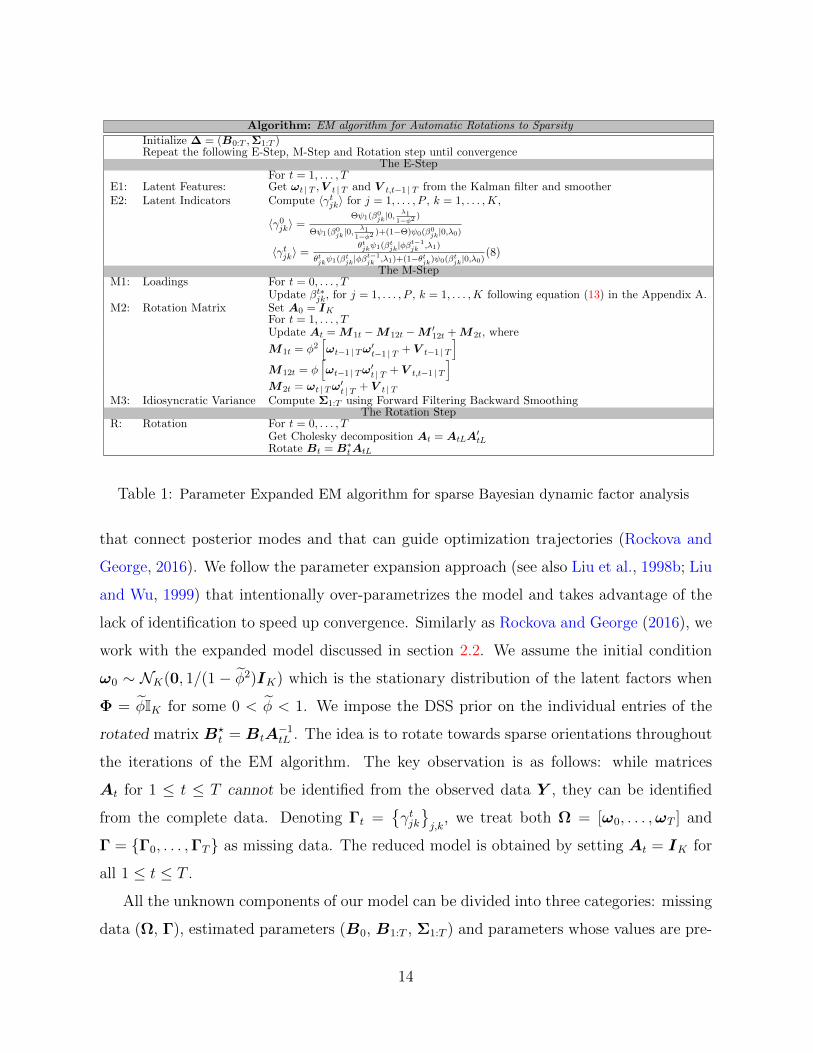
Algorithm: EM algorithm for Automatic Rotations to Sparsity

Initialize ∆ = (B0:T ,Σ1:T )Repeat the following E-Step, M-Step and Rotation step until convergence

The E-StepFor t = 1, . . . , T

E1: Latent Features: Get ωt | T ,V t | T and V t,t−1 | T from the Kalman filter and smootherE2: Latent Indicators Compute 〈γtjk〉 for j = 1, . . . , P , k = 1, . . . ,K,

〈γ0jk〉 =

Θψ1(β0jk|0,

λ11−φ2

)

Θψ1(β0jk|0,

λ11−φ2

)+(1−Θ)ψ0(β0jk|0,λ0)

〈γtjk〉 =θtjkψ1(βtjk|φβ

t−1jk ,λ1)

θtjkψ1(βtjk|φβt−1jk ,λ1)+(1−θtjk)ψ0(βtjk|0,λ0)

(8)

The M-StepM1: Loadings For t = 0, . . . , T

Update βt∗jk, for j = 1, . . . , P , k = 1, . . . ,K following equation (13) in the Appendix A.M2: Rotation Matrix Set A0 = IK

For t = 1, . . . , TUpdate At = M1t −M12t −M ′

12t +M2t, where

M1t = φ2[ωt−1 | Tω

′t−1 | T + V t−1 | T

]M12t = φ

[ωt−1 | Tω

′t | T + V t,t−1 | T

]M2t = ωt | Tω

′t | T + V t | T

M3: Idiosyncratic Variance Compute Σ1:T using Forward Filtering Backward SmoothingThe Rotation Step

R: Rotation For t = 0, . . . , TGet Cholesky decomposition At = AtLA

′tL

Rotate Bt = B∗tAtL

Table 1: Parameter Expanded EM algorithm for sparse Bayesian dynamic factor analysis

that connect posterior modes and that can guide optimization trajectories (Rockova and

George, 2016). We follow the parameter expansion approach (see also Liu et al., 1998b; Liu

and Wu, 1999) that intentionally over-parametrizes the model and takes advantage of the

lack of identification to speed up convergence. Similarly as Rockova and George (2016), we

work with the expanded model discussed in section 2.2. We assume the initial condition

ω0 ∼ NK(0, 1/(1 − φ2)IK) which is the stationary distribution of the latent factors when

Φ = φIK for some 0 < φ < 1. We impose the DSS prior on the individual entries of the

rotated matrix B?t = BtA

−1tL . The idea is to rotate towards sparse orientations throughout

the iterations of the EM algorithm. The key observation is as follows: while matrices

At for 1 ≤ t ≤ T cannot be identified from the observed data Y , they can be identified

from the complete data. Denoting Γt =γtjkj,k

, we treat both Ω = [ω0, . . . ,ωT ] and

Γ = Γ0, . . . ,ΓT as missing data. The reduced model is obtained by setting At = IK for

all 1 ≤ t ≤ T .

All the unknown components of our model can be divided into three categories: missing

data (Ω, Γ), estimated parameters (B0, B1:T , Σ1:T ) and parameters whose values are pre-

14

specified (φ, φ1, λ0, λ1, Θ and δ). Among the pre-specified parameters we set the AR

coefficients φ and φ1 close to (i.e. slightly smaller than) 1. This is because we want the

AR processes to be stationary but, at the same time, we do not want the current values to

deviate too far away from the past. We recommend setting values in the range [0.9, 1] for

the AR parameters. For similar reasons, the discount factor δ is also set close to unity (0.95

to be precise). However, instead of being treated as fixed values, the AR coefficients φ0

and φ1 can be easily estimated by assigning suitable priors, as demonstrated in the MCMC

implementation discussed in Section 3.2. Following the recommendation of (Rockova et al.,

2020), we set a moderate penalty for the spike distribution λ0 = 0.9 and a comparatively

large slab variance λ1 = 10(1−φ21). This is to ensure that the penalty on the factor loadings

is unimodal. The marginal importance weight Θ = 0.9 is chosen to be large because smaller

values provide an overwhelming support towards zero factor loadings.

Let us denote by ∆ = (B0,B1:T ,Σ1:T ) the model parameters. The matrix B0 contains

the initial conditions that are assumed to arise from the stationary spike-and-slab prior dis-

tribution and B1:T denotes all matrices Bt for 1 ≤ t ≤ T . The goal of the EM algorithm is

to find parameter values ∆, which are most likely (a posteriori) to have generated the data,

i.e. ∆ = arg max∆ log π(∆ | Y ). This is achieved indirectly by iteratively maximizing the

expectation of the augmented log-posterior, treating the hidden factors Ω and Γ as missing

data. Starting with an initialization ∆(0), the (m+ 1)st step of the EM algorithm outputs

∆(m+1) = arg max∆Q(∆ | ∆(m)), where Q(∆ | ∆(m)) = EΓ,Ω|Y ,∆(m) [log π(∆,Γ,Ω | Y )]

with EΓ,Ω|Y ,∆(m)(.) denoting the conditional expectation given the observed data and cur-

rent parameter estimates at the mth iteration. The EM algorithm iterates between the

E-step (obtaining the conditional expectation of the log-posterior) and the M-step (obtain-

ing ∆(m+1)). The parameter-expanded EM works in a slightly different manner.

The E-step of the parameter-expanded version operates in the reduced space (keeping

At = IK), while the M-step operates in the expanded space (allowing for general At).

Namely, the E-step computes the expectation Q(∆ |∆(m)) with respect to the conditional

distribution of Ω and Γ under the original model anchoring onBt andAt = IK , rather than

on B?t and unrestricted At. The M-step, on the other hand, is performed in the expanded

15

parameter space, where optimization takes place over B?0:T , Σ1:T , and A1:T . Updating

B?(m+1)0:T boils down to solving a series of independent penalized dynamic regressions. The

idiosyncratic variances Σt = diagσ21t, . . . , σ

2Pt for t = 1, . . . , T are estimated in the M-step

using Forward Filtering Backward Smoothing (Table 5 in the Appendix) (Ch. 4.3.7 Prado

and West, 2010) using the discount SV specification (as discussed in the Supplemental

Material). Since A1:T can be inferred from the complete data, one can estimate these

matrices in the M-step to leverage the information in the missing data. Nevertheless,

the updated matrices A1:T are not carried forward towards the next E-step (which uses

At = IK), but are used to rotate the solution B?(m+1)0:T back towards the reduced space via

B(m+1)t = B

?(m+1)t AtL. The steps of the algorithm are carefully explained in Section A.2.

The computations are summarized in Table 1. The convergence of the EM algorithm with

parameter expansion is provably faster (Liu et al., 1998b; Rockova and George, 2016).

3.2 MCMC

This section describes an MCMC algorithm for our dynamic factor model with dynamic

spike-and-slab priors. The DSS prior specification here is slightly different from the setup

considered for the EM algorithm. The Laplace spike distribution ψ0(β|λ0) = λ0/2e−λ0|β|

yields sparse posterior modes, a favorable feature for the EM algorithm. However, MCMC

ultimately reports the posterior mean which is non-sparse even under the Laplace prior. We

will therefore assume a Gaussian spike (instead of Laplace) to utilize its direct conditional

conjugacy for posterior updating. In particular, we assume the following spike density for

λ0 << λ1

ψ0(β | λ0) = exp−β2/(2λ0)/√

2πλ0. (9)

This yields the following conditional Gaussian distribution for individual factor loadings

βtjk

βtjk | γtjk, βt−1jk ∼ N

(γtjkµ

tjk , γ

tjkλ1 + (1− γtjk)λ0

)and transition weights θtjk in (6) with the Gaussian stationary spike distribution ψST0 (βt−1

jk |λ0) =

ψ0(β | λ0). An extension to the Laplace spike is possible with an additional augmentation

step, casting the Laplace distribution as a scale mixture of Gaussians with an exponential

16

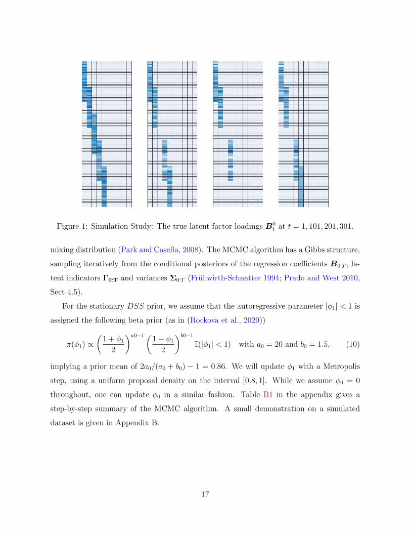
Figure 1: Simulation Study: The true latent factor loadings B0t at t = 1, 101, 201, 301.

mixing distribution (Park and Casella, 2008). The MCMC algorithm has a Gibbs structure,

sampling iteratively from the conditional posteriors of the regression coefficients B0:T , la-

tent indicators Γ0:T and variances Σ0:T (Fruhwirth-Schnatter 1994; Prado and West 2010,

Sect 4.5).

For the stationary DSS prior, we assume that the autoregressive parameter |φ1| < 1 is

assigned the following beta prior (as in (Rockova et al., 2020))

π(φ1) ∝(

1 + φ1

2

)a0−1(1− φ1

2

)b0−1

I(|φ1| < 1) with a0 = 20 and b0 = 1.5, (10)

implying a prior mean of 2a0/(a0 + b0) − 1 = 0.86. We will update φ1 with a Metropolis

step, using a uniform proposal density on the interval [0.8, 1]. While we assume φ0 = 0

throughout, one can update φ0 in a similar fashion. Table B1 in the appendix gives a

step-by-step summary of the MCMC algorithm. A small demonstration on a simulated

dataset is given in Appendix B.

17

4 Simulation Study

We illustrate the usefulness of our proposed approach, relative to multiple existing methods,

on synthetic data reflecting the following characteristics that can occur in real applications:

dynamic patterns of sparsity, smoothness, and a time-varying factor dimension.

First, we generate a single dataset with P = 100 responses, K = 10 candidate latent

factors, and T = 400 time series observations (extra 100 data points are generated as train-

ing data for the rolling window analysis, as will be described below). The dimensionality of

this example is already beyond practical limits of many Bayesian procedures. The elements

of latent factors Ωt and idiosyncratic errors εt are generated from a standard Gaussian dis-

tribution. Only the first five factors are potentially active over time, with the latter five

being always inactive. We now describe the true loading matrices B0 = [B01, . . . ,B

0T ],

which were used to generate the data, where B0t = β0t

jk ∈ RP×K . At time t = 1, the

active latent factor loadings form a block diagonal structure with 28 active loadings per

factor, of which 10 overlap with another factor. In other words, we have 60 series with

only one active factor, and 40 with two active factors (see the leftmost image in Figure 1).

The sparsity pattern changes structurally over time where (a) at time t = 101 the loadings

of the third factor become inactive, (b) at t = 201 the loadings of the fifth factor become

inactive, and (c) at t = 301 the loadings of the fifth factor are re-introduced and active

until T = 400 (Figure 1). The true nonzero loadings are smooth and arrive from an au-

toregressive process, i.e. β0tjk = φβ0t−1

jk + vtjk with vtjkiid∼ N (0, 0.0025) for φ = 0.99, initiated

at β01jk = 2 for all 1 ≤ j ≤ P and 1 ≤ k ≤ 5. When loadings β0t

jk become inactive, they are

thresholded to zero. The true factor loadings are thereby smooth until they suddenly drop

out and can emerge.

We compare our proposed dynamic spike-and-slab factor selection with three other

approaches. The first one is the “rolling window” version of the static factor analysis with

rotations to sparsity by Rockova and George (2016) using K = 10 (i.e. overshooting the

true factor dimensionality). We compare this approach with “Adaptive PCA” of Bai and

Ng (2002), which corresponds to a rolling-window principal component analysis (PCA)

with estimated number of factors, and with “Sparse PCA” using K = 10, which is a

18

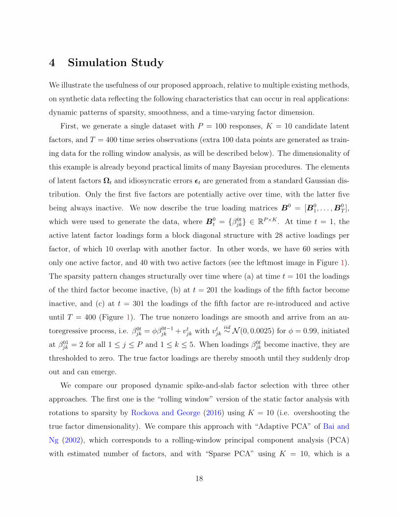
(a) t = 100

(b) t = 200

(c) t = 300

(d) t = 400

Figure 2: Simulated Example: Heatmaps of true and estimated factor loadings at t =

100, 200, 300, 400. Comparisons are made between (from left to right), the true factor

loadings, “Adaptive PCA,” “Sparse PCA” (K = 10), rolling window spike-and-slab factor

analysis (K = 10), and our dynamic spike-and-slab factor analysis. The first three methods

are estimated using a rolling window of 100 data points. Factor loadings are absolute and

capped at 0.5 for visibility. 19

rolling-window LASSO-based regularization method with cross-validation for selecting the

level of shrinkage (Witten et al., 2009). All these methods are estimated using a rolling

window of size 100, where we generate extra 100 training data points using the sparsity

pattern B01. We choose Φ = φIK with φ = 0.95 and K = 10. Choosing φ close to 1 ensures

that the latent factor processes are stationary and their means do not deviate too far away

from past values. To deploy the dynamic spike-and-slab priors, we set φ0 = 0, φ1 = 0.98,

λ0 = 0.9, λ1 = 10(1 − φ21), and Θ = 0.9. To improve the performance of our EM method,

we initialize the procedure using the output from the rolling window static spike-and-slab

factor model of Rockova and George (2016).

Focusing on the reconstruction of factor loadings, we take snapshots at times t =

100, 200, 300, 400 and visually compare the output to the truth (Figure 2). We see that

both spike-and-slab methods achieve good recovery. However, the static spike-and-slab

cannot fully contain the dynamic loadings, where we see a lot of spillover to other factors.

Dynamic spike-and-slab shrinkage, on the other hand, smooths out the sparsity over time,

clearly improving on the recovery. “Adaptive PCA” performs well, correctly specifying the

number of factors. However, the factor loadings are non-sparse and rotated. “Sparse PCA”

with K = 10 is fairly successful, recovering the blocking structure correctly, but splitting

the signal among multiple factors (an observation made also by Rockova and George,

2016). For the spike-and-slab methods, these patterns can be alternatively obtained by

thresholding conditional inclusion probabilities rather than just looking at nonzero entries

in B1:T .

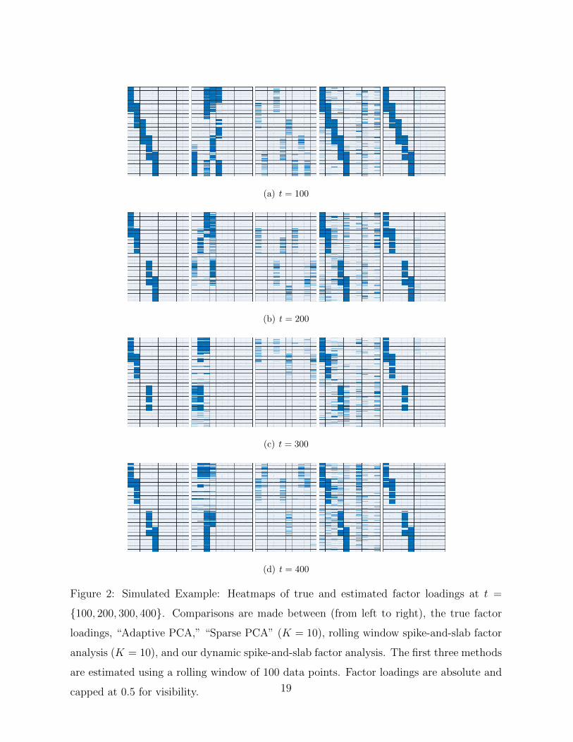
We further explore how the root mean squared errors (RMSE) change over time for one

of the simulations (Figure 3). This is calculated for each t = 1 : T by

RMSE(Bt) =

√tr(B0

t − Bt)′(B0t − Bt)

P ×K, (11)

where Bt are the estimated factor loadings at time t. Since this comparison is not entirely

meaningful due to the rotational invariance, we compute (11) for the left-ordered variants of

these matrices. By looking at the speed of decrease in RMSE after a structural change, it is

clear that dynamic spike-and-slab adapts faster compared to its rolling window counterpart.

The drop of RMSE for “Adaptive PCA” in periods 101:200 and 201:300 can be attributed

20

(a) RMSE (b) K

Figure 3: Simulation Study: (Left) The root mean squared error (11) and (Right) the

estimated number of factors for “Adaptive PCA,” “Sparse PCA,” static spike-and-slab,

and dynamic spike-and-slab, calculated for each t = 1:400.

to the fact that the number of factors was estimated correctly, resulting in many true zero

discoveries. On the other hand, the large estimation error of “Sparse PCA” is due to the

lack of sparsity and scattered structure of the factors.

Additionally, we plot the estimated number of factors for each method and compare it

to the true number of factors. “Sparse PCA” overestimates the number of factors (where

we regard a factor as active if it has at least one nonzero loading). This indicates that

unstructured sparsity is not enough. Looking at “Adaptive PCA” and our dynamic spike-

and-slab factor model, we find that both perform similarly well in terms of estimating the

number of factors. Furthermore, we note that dynamic spike-and-slab adapts faster to

factors disappearing, while “Adaptive PCA” adapts faster to factors reappearing.

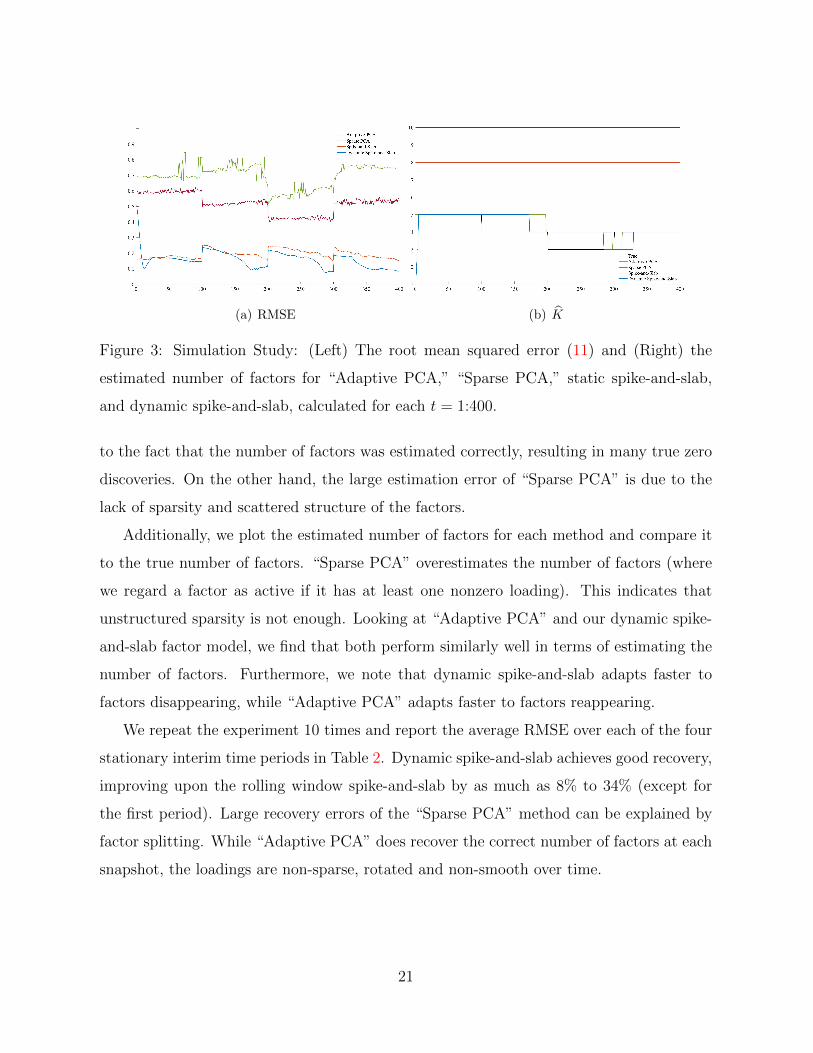
We repeat the experiment 10 times and report the average RMSE over each of the four

stationary interim time periods in Table 2. Dynamic spike-and-slab achieves good recovery,

improving upon the rolling window spike-and-slab by as much as 8% to 34% (except for

the first period). Large recovery errors of the “Sparse PCA” method can be explained by

factor splitting. While “Adaptive PCA” does recover the correct number of factors at each

snapshot, the loadings are non-sparse, rotated and non-smooth over time.

21

t=1:100 t=101:200 t=201:300 t=301:400

RMSE % K RMSE % K RMSE % K RMSE % K

Adaptive PCA 1.0660 -266.07 5 1.0590 -400.24 4.97 0.9730 -250.38 3.97 1.033 -430.01 3.88

Sparse PCA 0.7862 -169.99 10 0.7260 -242.94 10 0.6377 -129.64 10 0.7383 -278.81 10

Spike-and-Slab 0.1919 34.10 8 0.2843 -34.29 8 0.2988 -7.60 8 0.2447 -25.60 8

Dynamic Spike-and-Slab 0.2912 - 4.89 0.2117 - 4.72 0.2777 - 3.84 0.1949 - 3.71

Table 2: Simulation Study: Performance evaluation of the latent factor methods compared to the

true coefficients for t = 1:400. Performance is evaluated based on RMSE within each evaluation

period. % is the performance gain compared to dynamic spike-and-slab. K is the average number

of factors estimated during that period.

5 Empirical Study

The empirical application concerns a large-scale monthly U.S. macroeconomic database,

(colloquially known as the FRED-MD dataset (McCracken and Ng, 2016) in the Macroe-

conomics literature) comprising a balanced panel of P = 127 monthly macroeconomic

and financial variables tracked over the period of 2001/01 to 2015/12 (T = 180). These

variables are classified into eight main categories, depending on their economic meaning:

Output and Income, Labor Market, Consumption and Orders, Orders and Inventories,

Money and Credit, Interest Rate and Exchange Rates, Prices, and Stock Market. A de-

tailed description of how variables were collected and constructed is provided in McCracken

and Ng (2016). A quick table of names and groups of each variable is in the Appendix

(Table B3). The variables were centered to have mean zero and standardized following the

procedures in McCracken and Ng (2016).

This data, and its various subsets, have been widely studied in the literature, either

as a standalone dataset (for macroeconomic forecasting and an impulse/response analysis)

or as an essential part of broader data contexts. We review these analyses briefly below.

For example, Stock and Watson (2018) deployed this dataset for estimation of dynamic

causal effects in Macroeconomics. In other analyses, Miranda-Agrippino and Ricco (2018)

extracted a set of lagged macro-financial dynamic factors to project monetary policy shocks

and Gargano et al. (2019) computed the Ludvigson-Ng (LN) macro factors for predicting

bond values. Using a quarterly aggregated version of this data, Huber and Feldkircher

22

(2019) fitted a Bayesian vector autoregressive model to forecast a subset of 21 variables.

A larger forecasting exercise was conducted by Koop et al. (2019), who used 129 variables

spanning over years 1960 to 2014 to predict GDP growth, inflation and short-term interest

rates. A subset of this data, in conjunction with additional economic variables has been

analyzed in Daniele and Schnaitmann (2019) who study the effects of a monetary policy

shock through a regularized factor-augmented vector autoregressive (FAVAR) model. While

the central theme of these works has been forecasting and/or impulse response analysis, the

primary focus of our analysis in this section is discovering latent interpretable structures and

glean insights into the interconnectivity between different sectors of the US macroeconomy,

with a particular focus on the 2008 financial crisis. Forecasting will be discussed later in

Section 6.

Stock and Watson (2005) analyzed a similar macroeconomic dataset (often referred to

as the “Stock and Watson” dataset in Econometrics literature), containing 132 series over

the sample 1959:1 to 2003:12. After performing variance decompositions, they found six

factors that explain most of the variation in the data. With the same dataset, the IC1

and IC2 criteria developed in Bai and Ng (2002) find seven static factors explaining over

40 percent of the variation in the data. Bai and Ng (2013) used the same data extended

to 2007:12 and showed first 7 factors still explain 45 percent of the variation in the data,

though the IC2 criterion found the optimal number of factors to be 8.

The purpose of conducting a sparse latent factor analysis on a large-scale economic

dataset, such as this one, is at least twofold. Due to the group structure of the data, it is

natural to assume that the measured indicators are tied via a few latent factors, the basic

premise of latent factor modeling. Moreover, we expect the sparse latent structure to detect

clusters of dependence structures that capture the interconnectivity of indicators spanning

many different aspects of the economy. Sparsity will help extract such interpretable struc-

tures. Second, given the dynamic nature of the economy, there is a substantial interest

in understanding how these dependencies change over time and– in particular– how they

are affected by shocks. We anticipate non-negligible shifts in the economy, as the data

spans over the housing bubble deflation after 2006 and the great financial crisis in late

23

2008, which led to the Great Recession. Understanding the interplay between contribut-

ing factors to the financial crisis has been a subject of rigorous research (see for example,

Benmelech et al., 2017; Chodorow-Reich, 2014; Commission, 2011; Mian et al., 2013; Mian

and Sufi, 2009, 2011; Reinhart and Rogoff, 2008). Our analysis is purely data-driven and

thereby descriptive rather than causally conclusive. We attempt to characterize patterns of

shock proliferation and permanence of structural changes of the economy using our dynamic

factor model.

As the dataset is considerably richer than our simulated example, we expand the model

(1) by incorporating a dynamic intercept to capture location shifts that could not be easily

standardized away. The intercepts cjt follow independent random walk evolutions with

an initial condition c0 ∼ N(0, 1). The initial condition for the SV variances is 1/σ2j0

ind∼

G(n0/2, d0/2) for 1 ≤ j ≤ P with n0 = 20 and d0 = 0.002. The discount factor is set to

0.95.

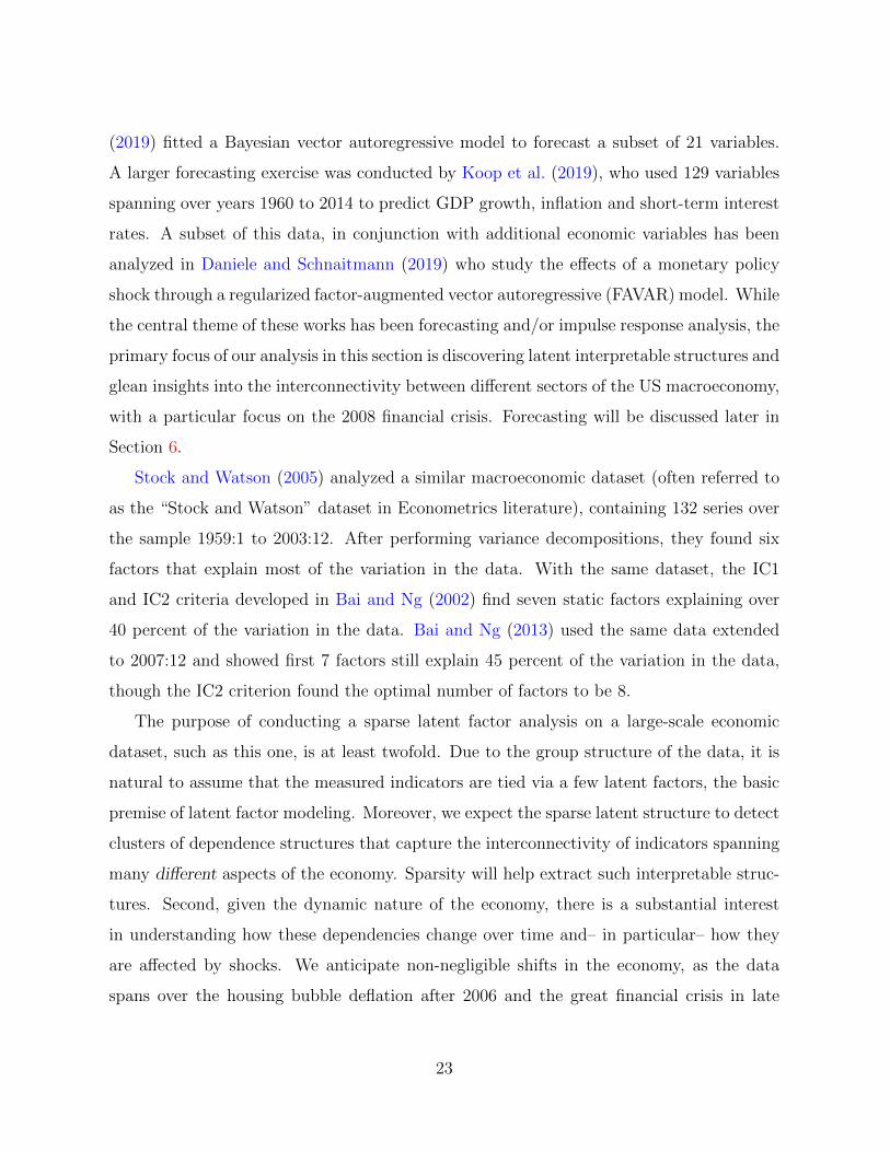
First, we examine one snapshot of the output from “Adaptive PCA” and “Sparse PCA”

(described in Section 4) at time 2015/12 (Figures 4). Both methods do pick up certain

groupings, but do not yield interpretable enough representations. This is likely due to

overestimation of the number of factors (Figure 4 (b)), factor rotation and lack of sparsity

(Figure 4 (a)) and/or factor splitting (Figure 4 (c)). Next, we deploy the rolling window

spike-and-slab factor method with a training period of 10 years to obtain starting values

for our dynamic factor model. Priors and their hyper-parameters were chosen as in the

simulation study. We choose a generous upper bound K = 126 on the number of factors,

letting the sparsity rule out factors that are irrelevant.

We now examine the output of our procedure at three time points: 2003/12, 2008/10,

and 2015/12. These three snapshots are of particular interest as they represent three dis-

tinct states of the economy: relative stability (2003), sharp economic crisis (2008), and

recovery (2015). 2008/10 is at the onset of the great financial crisis, where deflation of

the housing bubble after 2006 lead to mortgage delinquencies and financial fragility (Com-

mission, 2011). This distress permeated throughout the rest of the economy, including the

labor market, leading to the deepest recession in the post-war history.

24

(a) “Adaptive PCA” (b) ”Sparse PCA” (c) ”Sparse PCA”

Figure 4: Macroeconomic Study: Estimated factor loadings using “Adaptive PCA” (Left),

“Sparse PCA” with number of factors set as 30 (Middle), and “Sparse PCA” with number

of factors set to 8 from the results of “Adaptive PCA” (Right) at t = 2015/12, with the

number of series on the y-axis and the number of factors in the x-axis. The factor loading

are estimated using a 10 year rolling window.

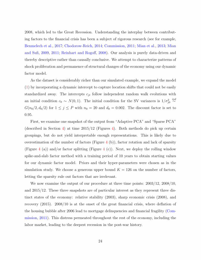
The heatmap of estimated factor loadings at time 2003/12 is in Figure 5 (left). The

output has been left-ordered based on the results at 2015/12, where the more active factors

are on the left, in the order of data series, and some of the less active right-most factors

(with small or zero loadings) are omitted. There are 24 active factors in total (i.e. factors

with at least two non-negligible non-zero factor loadings), with only 5 factors that cluster

eight or more series (Factors 2, 10, 22, 23, and 25). Since the variables are grouped by their

economic meaning, this type of clustering is not entirely unexpected. For example, Fac-

tor 2 includes CMRMTSPLx (real manufacturing and trade industry sales), all industrial

production indices except nondurable materials, residential utilities, and fuels, CUMFNS

(capacity utilization), DMANEMP (durable goods employment), and ISRATIOx (manu-

facturing and trade inventories to sales ratio). This factor could be interpreted as a factor

for durable goods, which include industries that are more susceptible to economic trends,

25

Figure 5: Macroeconomic Study: Estimated factor loadings using dynamic sparse factor

analysis at t = 2003/12 (left), t = 2008/10 (center), t = 2015/12 (right), with the orig-

inal series on the y-axis and the factors in the x-axis. The factor loading are estimated

dynamically over the period 2001/1:2015/12.

where sales, inventories, industrial production, capacity utilization, and employment are

all connected. Conversely, we expect nondurable goods, such as utilities and fuels, to have

a different dynamic than durable goods, which is reflected in the exclusion of those in-

dices in Factor 2. Similarly, Factor 10 includes employment data (except for mining and

logging, manufacturing, durable goods, nondurable goods, and government), Factor 22 in-

cludes interests rates (fed funds rate, treasury bills, and bond yields), Factor 23 includes

the spread between interest rates minus fed funds rate, and Factor 25 includes consumer

price indices except apparel, medical care, durables, and services, as well as personal con-

sumptions expenditures on nondurable goods. All of these factors produce meaningful and

mostly separated clusters that largely conform with economic intuition.

During the crisis (Figures 5; center), radical changes occur in the factor structure.

26

Concerning Factor 2, the dependence structure expands, now spanning over nondurables

and fuels, as well as HWI (the help wanted index), UNEMP15OV (unemployment for 15

weeks and over), CLAIMSx (unemployment insurance claims), and PAYEMS (employment,

total non-farm, goods-producing, manufacturing, and durable goods). This indicates that

the shock might have affected relatively stable industries and unemployment, with the co-

movement across industries being largely synchronized under distress (with the exception

of residential utilities). Another interesting observation is the emergence of new factors. In

particular, Factor 11, which includes housing starts and new housing permits in different

regions in the U.S., was not present pre-crisis and now surfaces as a connecting thread

between housing markets across regions. While in 2003/12 the latent factors were largely

separated (loadings had little overlap), we now see at least two factors (namely Factor 25

and 28), whose loadings are non-sparse and far-reaching. In particular, Factor 28 emerges

as a non-sparse link between many different sectors of the economy, including retail sales,

industrial production, employment (in particular financial services), real M2 money stock,

loans, BAA bond yields (but not AAA), exchange rates, consumer sentiment, investment

and, most importantly, the stock market indices, including the S&P 500 and the VIX

(i.e. the fear index), a popular measure of the stock market’s expectation of volatility.

This factor loads heavily on stock market indices, which were isolated pre-crisis, but are

now connected to the various corners of the economy. Factor 25, on the other hand, is

driven mainly by prices (e.g. CPI). Both of these factors could potentially be interpreted

as crisis factors as they permeate through various sectors of the economy, that had little

interconnectivity in the pre-crisis era. The only sectors not influenced by these factors are

Consumption and Orders and, more interestingly, the housing market.

There is an ongoing discussion on what were the main catalysts of the Great Recession.

One line of reasoning focuses on the financial market, where the devaluation of securities,

including mortgage backed securities, led to curtailed lending and thereby consumption

(Benmelech et al., 2017; Chodorow-Reich, 2014). The second one focuses directly on the

downturn of the housing market (Mian et al., 2013; Mian and Sufi, 2009, 2011). The

“orthogonality” between the housing market factor (Factor 11) and the “crisis factors”

27

(Factor 25 and 28) may suggest that, while the crisis was triggered by the housing market,

the main catalyst of the recession was probably the financial market. While our analysis

does not necessarily prove this hypothesis, it aligns with the previous lines of reasoning.

Finally, Figure 5 (right) shows the end of the analysis at 2015/12, where the economy

has mostly recovered from the Great Recession, but has fundamentally changed from what

it was before. Although most of the factor overlap has dissipated, we see a notably different

structure compared to 2003. In particular, Factor 5 (employment) and Factor 11 (housing)

persevere from the crisis. Moreover, the “crisis factors” Factor 25 and 28, representing

the prices and the stock market, are no longer strongly tied to other parts of the economy

(labor, output, interest and exchange rates, etc.). In addition, the VIX indicator for market

sentiment, is no longer connected to many of the key factors, even the stock market, and

is only connected to Factor 5, implying that the market’s anticipation of volatility is no

longer severely intertwined with the rest of the economy. Factor 2 is one of the few factors

that have returned back to its original structure, except for CMRMTSPLx and industrial

production of nondurable consumer goods. Its dependence with the labor market (e.g.

unemployment) has disappeared, suggesting that industry production is no longer in co-

movement with the labor market.

We also obtain insights into the effects and duration of the crisis by looking at the

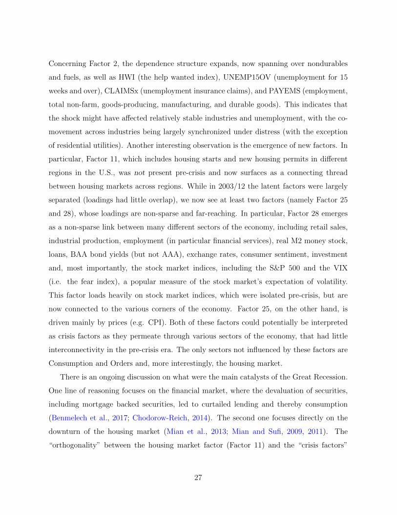
evolution of the factor loadings for one of the “crisis” factors, Factor 28. Figure 6 shows a

dynamic heatmap and a 3-D plot of βtjk for 1 ≤ j ≤ 127 (y-axis) and 1 ≤ t ≤ 180 (x-axis)

with k = 28. For the 3-D plot, the loadings on the S&P indices are suppressed to zero in

order to improve visibility. The figure reveals a spur of activity around the sharp financial

crisis (late 2008 and early 2009), where the contagion battered multiple corners of the

economy. The duration of the active loadings provide additional insights. For example, the

loadings on VIX (series 127) emerges and disappears in a eight month span from 06/2008

to 02/2009, while the loadings on the exchange rate between U.S. and Canada lasts for 17

months. However, most factor loadings seem to only emerge for about 4-6 months.

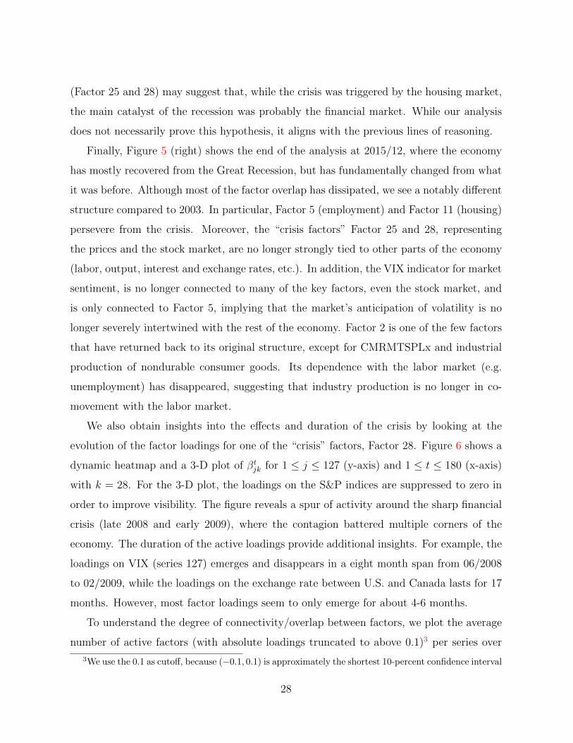
To understand the degree of connectivity/overlap between factors, we plot the average

number of active factors (with absolute loadings truncated to above 0.1)3 per series over

3We use the 0.1 as cutoff, because (−0.1, 0.1) is approximately the shortest 10-percent confidence interval

28

Figure 6: Macroeconomic Study: Estimated factor loadings for Factor 28 using dynamic

spike-and-slab from t = 2001/12:2015/12, with a heatmap of the entire factor loadings

(Left) and a 3-D plot of the factor loadings with the loadings on 123-126 (S&P related

indices) set to zero to increase visibility.

time (Figure 7). More overlap indicates a more intertwined economy. We observe an

increase in late 2008, reflecting the emergence of pervasive crisis factor(s), as well as its

build up from mid-2006. Another point to note is that the level pre-crisis is comparatively

lower than post-crisis, indicating a structural shift is the economy brought on by the crisis.

We further our analysis with a few insights into the idiosyncratic variances for variables

related to the housing market: HOUST (total housing starts) and its regional variants

(North East, Mid-West, South, and West). We choose the housing market for deeper anal-

ysis, because the housing market has been subjected to intense scrutiny, following the great

recession of 2009, as a suspected trigger of the crisis (Mian et al., 2013; Mian and Sufi, 2009,

2011). Housing starts is the seasonally adjusted number of new residential construction

projects that have begun during any particular month and, as such, is a key part of the U.S.

economy, which relates to employment and many industry sectors including banking (the

mortgage sector), raw materials production, construction, manufacturing, and real estate.

of the spike distribution (Laplace distribution centered at 0 and with variance being equal to 0.9) used in

the dynamic spike and slab prior.

29

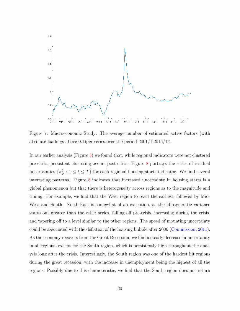
Figure 7: Macroeconomic Study: The average number of estimated active factors (with

absolute loadings above 0.1)per series over the period 2001/1:2015/12.

In our earlier analysis (Figure 5) we found that, while regional indicators were not clustered

pre-crisis, persistent clustering occurs post-crisis. Figure 8 portrays the series of residual

uncertainties σ2jt : 1 ≤ t ≤ T for each regional housing starts indicator. We find several

interesting patterns. Figure 8 indicates that increased uncertainty in housing starts is a

global phenomenon but that there is heterogeneity across regions as to the magnitude and

timing. For example, we find that the West region to react the earliest, followed by Mid-

West and South. North-East is somewhat of an exception, as the idiosyncratic variance

starts out greater than the other series, falling off pre-crisis, increasing during the crisis,

and tapering off to a level similar to the other regions. The speed of mounting uncertainty

could be associated with the deflation of the housing bubble after 2006 (Commission, 2011).

As the economy recovers from the Great Recession, we find a steady decrease in uncertainty

in all regions, except for the South region, which is persistently high throughout the anal-

ysis long after the crisis. Interestingly, the South region was one of the hardest hit regions

during the great recession, with the increase in unemployment being the highest of all the

regions. Possibly due to this characteristic, we find that the South region does not return

30

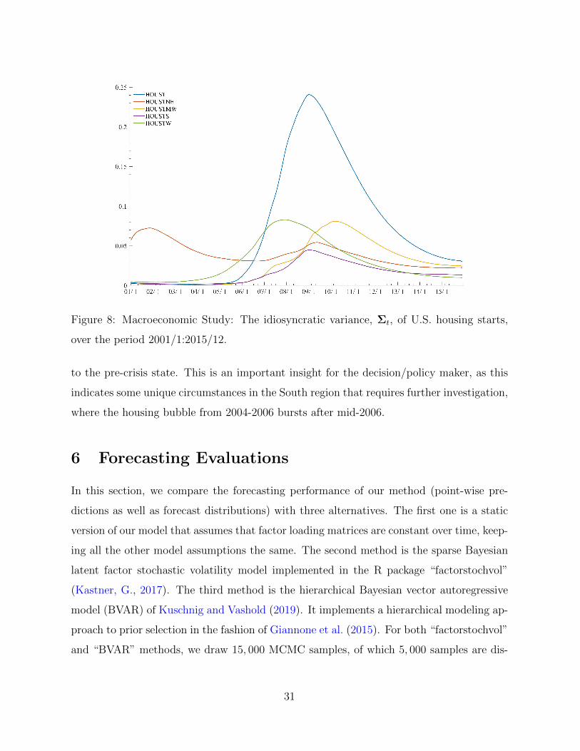
Figure 8: Macroeconomic Study: The idiosyncratic variance, Σt, of U.S. housing starts,

over the period 2001/1:2015/12.

to the pre-crisis state. This is an important insight for the decision/policy maker, as this

indicates some unique circumstances in the South region that requires further investigation,

where the housing bubble from 2004-2006 bursts after mid-2006.

6 Forecasting Evaluations

In this section, we compare the forecasting performance of our method (point-wise pre-

dictions as well as forecast distributions) with three alternatives. The first one is a static

version of our model that assumes that factor loading matrices are constant over time, keep-

ing all the other model assumptions the same. The second method is the sparse Bayesian

latent factor stochastic volatility model implemented in the R package “factorstochvol”

(Kastner, G., 2017). The third method is the hierarchical Bayesian vector autoregressive

model (BVAR) of Kuschnig and Vashold (2019). It implements a hierarchical modeling ap-

proach to prior selection in the fashion of Giannone et al. (2015). For both “factorstochvol”

and “BVAR” methods, we draw 15, 000 MCMC samples, of which 5, 000 samples are dis-

31

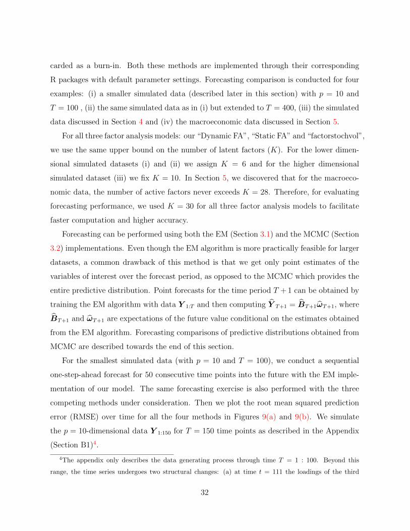
carded as a burn-in. Both these methods are implemented through their corresponding

R packages with default parameter settings. Forecasting comparison is conducted for four

examples: (i) a smaller simulated data (described later in this section) with p = 10 and

T = 100 , (ii) the same simulated data as in (i) but extended to T = 400, (iii) the simulated

data discussed in Section 4 and (iv) the macroeconomic data discussed in Section 5.

For all three factor analysis models: our “Dynamic FA”, “Static FA” and “factorstochvol”,

we use the same upper bound on the number of latent factors (K). For the lower dimen-

sional simulated datasets (i) and (ii) we assign K = 6 and for the higher dimensional

simulated dataset (iii) we fix K = 10. In Section 5, we discovered that for the macroeco-

nomic data, the number of active factors never exceeds K = 28. Therefore, for evaluating

forecasting performance, we used K = 30 for all three factor analysis models to facilitate

faster computation and higher accuracy.

Forecasting can be performed using both the EM (Section 3.1) and the MCMC (Section

3.2) implementations. Even though the EM algorithm is more practically feasible for larger

datasets, a common drawback of this method is that we get only point estimates of the

variables of interest over the forecast period, as opposed to the MCMC which provides the

entire predictive distribution. Point forecasts for the time period T + 1 can be obtained by

training the EM algorithm with data Y 1:T and then computing Y T+1 = BT+1ωT+1, where

BT+1 and ωT+1 are expectations of the future value conditional on the estimates obtained

from the EM algorithm. Forecasting comparisons of predictive distributions obtained from

MCMC are described towards the end of this section.

For the smallest simulated data (with p = 10 and T = 100), we conduct a sequential

one-step-ahead forecast for 50 consecutive time points into the future with the EM imple-

mentation of our model. The same forecasting exercise is also performed with the three

competing methods under consideration. Then we plot the root mean squared prediction

error (RMSE) over time for all the four methods in Figures 9(a) and 9(b). We simulate

the p = 10-dimensional data Y 1:150 for T = 150 time points as described in the Appendix

(Section B1)4.

4The appendix only describes the data generating process through time T = 1 : 100. Beyond this

range, the time series undergoes two structural changes: (a) at time t = 111 the loadings of the third

32

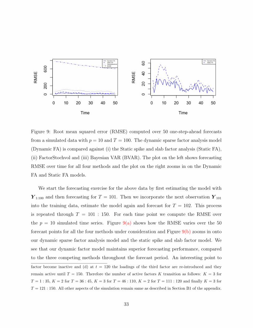
Figure 9: Root mean squared error (RMSE) computed over 50 one-step-ahead forecasts

from a simulated data with p = 10 and T = 100. The dynamic sparse factor analysis model

(Dynamic FA) is compared against (i) the Static spike and slab factor analysis (Static FA),

(ii) FactorStochvol and (iii) Bayesian VAR (BVAR). The plot on the left shows forecasting

RMSE over time for all four methods and the plot on the right zooms in on the Dynamic

FA and Static FA models.

We start the forecasting exercise for the above data by first estimating the model with

Y 1:100 and then forecasting for T = 101. Then we incorporate the next observation Y 101

into the training data, estimate the model again and forecast for T = 102. This process

is repeated through T = 101 : 150. For each time point we compute the RMSE over

the p = 10 simulated time series. Figure 9(a) shows how the RMSE varies over the 50

forecast points for all the four methods under consideration and Figure 9(b) zooms in onto

our dynamic sparse factor analysis model and the static spike and slab factor model. We

see that our dynamic factor model maintains superior forecasting performance, compared

to the three competing methods throughout the forecast period. An interesting point to

factor become inactive and (d) at t = 120 the loadings of the third factor are re-introduced and they

remain active until T = 150. Therefore the number of active factors K transition as follows: K = 3 for

T = 1 : 35, K = 2 for T = 36 : 45, K = 3 for T = 46 : 110, K = 2 for T = 111 : 120 and finally K = 3 for

T = 121 : 150. All other aspects of the simulation remain same as described in Section B1 of the appendix.

33

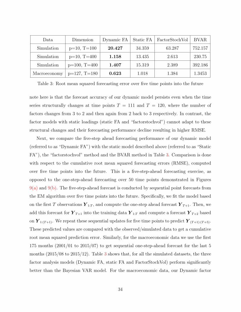
Data Dimension Dynamic FA Static FA FactorStochVol BVAR

Simulation p=10, T=100 20.427 34.359 63.287 752.157

Simulation p=10, T=400 1.158 13.435 2.613 230.75

Simulation p=100, T=400 1.407 15.319 2.389 392.186

Macroeconomy p=127, T=180 0.623 1.018 1.384 1.3453

Table 3: Root mean squared forecasting error over five time points into the future

note here is that the forecast accuracy of our dynamic model persists even when the time

series structurally changes at time points T = 111 and T = 120, where the number of

factors changes from 3 to 2 and then again from 2 back to 3 respectively. In contrast, the

factor models with static loadings (static FA and “factorstochvol”) cannot adapt to these

structural changes and their forecasting performance decline resulting in higher RMSE.

Next, we compare the five-step ahead forecasting performance of our dynamic model

(referred to as “Dynamic FA”) with the static model described above (referred to as “Static

FA”), the “factorstochvol” method and the BVAR method in Table 3. Comparison is done

with respect to the cumulative root mean squared forecasting errors (RMSE), computed

over five time points into the future. This is a five-step-ahead forecasting exercise, as

opposed to the one-step-ahead forecasting over 50 time points demonstrated in Figures

9(a) and 9(b). The five-step-ahead forecast is conducted by sequential point forecasts from

the EM algorithm over five time points into the future. Specifically, we fit the model based

on the first T observations Y 1:T , and compute the one-step ahead forecast Y T+1. Then, we

add this forecast for Y T+1 into the training data Y 1:T and compute a forecast Y T+2 based

on Y 1:(T+1). We repeat these sequential updates for five time points to predict Y (T+1):(T+5).

These predicted values are compared with the observed/simulated data to get a cumulative

root mean squared prediction error. Similarly, for the macroeconomic data we use the first

175 months (2001/01 to 2015/07) to get sequential one-step-ahead forecast for the last 5

months (2015/08 to 2015/12). Table 3 shows that, for all the simulated datasets, the three

factor analysis models (Dynamic FA, static FA and FactorStochVol) perform significantly

better than the Bayesian VAR model. For the macroeconomic data, our Dynamic factor

34

analysis model appears to perform considerably better than the alternatives. This reiterates

the merits of using dynamic factor loadings as opposed to constant loading matrices.

The above observations are confirmed after computing the one-step-ahead log predictive

density scores (LPDS) measuring the quality of the entire forecast distributions. For this

forecasting comparison, we use our MCMC implementation (Section 3.2). As described by

Kastner (2019), the one step ahead LPDS for the dynamic factor model can be computed

by first drawing M MCMC samples from the distribution of Y1:T and then averaging over

m = 1, . . . ,M densities of

Np(0,B

(m)(T+1):[1:T ]B

(m)′

(T+1):[1:T ] + Σ(m)(T+1):[1:T ]

)evaluated at Y T+1, where B

(m)T+1:[T+1] and Σ

(m)(T+1):[1:T ] denote the m-th draw of BT+1 and

ΣT+1 respectively, from the posterior distribution up to time T . Next, we compute the

one-step ahead log predictive Bayes factor between our dynamic factor model and the static

spike-and-slab factor model. Such Bayes factor between any two models M1 and M2 is

defined as logBF (M1,M2) = logPLT+1(M1)− logPLT+1(M2), where PLt(M) denotes

the predictive likelihood of modelM at time T +1. When the log predictive Bayes factor is

greater than zero at a given point in time, there is evidence in favor of modelM1 as opposed

to model M2, and vice versa. For the simulated examples with p = 10 and T = 100, the

Bayes factor computed between our dynamic factor model and the static factor model turn

out to be equal to

logBF (Dynamic FA, Static FA) = 2.161

implying (strong) evidence in favor of the dynamic sparse factor model.

7 Further Comments

Motivated by a topical macroeconomic dataset, we developed a Bayesian method for dy-

namic sparse factor analysis for large-scale time series data. Our proposed methodology

aims to tackle three challenges of dynamic factor analysis: time-varying patterns of sparsity,

unknown number of factors, and identifiability constraints. By deploying dynamic sparsity,

35

we successfully recover interpretable latent structures that automatically select the number

of factors and that incorporate time-varying loadings/factors. We successfully applied our

methodology on a nontrivial simulated example as well as a real dataset comprising of 127

U.S. macroeconomic indices tracked over the period of the Great Recession (and beyond)

and obtained several interpretable findings.

Our methodology can be enriched/extended in many ways. One possible extension

would be to develop a latent variable method that can capture within, as well as between,

connectivity of several high-dimensional time series. This could be achieved with a dynamic

extension of sparse canonical correlation analysis (Witten et al., 2009). Our method can

also be embedded within FAVAR models (Bernanke et al., 2005) that include both observed

and unobserved predictors. Additionally, throughout our analysis we have assumed the

covariance of the latent factors to be fixed over time and equal to an identity matrix, one

could in principle incorporate dynamic variances with stochastic volatility modeling, along

the lines of Zhou et al. (2014).

One possible shortcoming of our EM-based estimation strategy, is the lack of uncer-

tainty assessment, which is essential for forecasting. The EM algorithm, however, was

the key to obtaining interpretable latent structures for very high dimensional data. To

achieve uncertainty quantification along with interpretability, one could impose structural

identification constraints, such as Nakajima and West (2013a,b), and perform MCMC for

DSS priors, as demonstrated in Appendix B. Another approach would be to apply our

method simply as a means of obtaining identifiability constraints (i.e. the sparsity pattern)

and then reestimate the nonzero loadings with an MCMC strategy. While this would not

quantify any sparsity-selection uncertainty, it would be an effective way to balance inter-

pretability and forecasting/decision making. Another unavoidable feature of our method is

its sensitivity to starting values. We strongly recommend using the output from the rolling

window spike-and-slab factor model.

36

References

Aguilar, O., G. Huerta, R. Prado, and M. West (1998). Bayesian inference on latent

structure in time series. Bayesian Statistics 6 (1), 1–16.

Aguilar, O. and M. West (1998). Bayesian dynamic factor models and variance matrix

discounting for portfolio allocation. Institute of Statistics and Decision Sciences, Duke

University.

Aguilar, O. and M. West (2000). Bayesian dynamic factor models and portfolio allocation.

Journal of Business & Economic Statistics 18 (3), 338–357.

Aunsri, N. and P. Taveeapiradeecharoen (2020). A time-varying bayesian compressed vector

autoregression for macroeconomic forecasting. IEEE Access 8, 192777–192786.

Bai, J. and S. Ng (2002). Determining the number of factors in approximate factor models.

Econometrica 70 (1), 191–221.

Bai, J. and S. Ng (2013). Principal components estimation and identification of static

factors. Journal of Econometrics 176 (1), 18–29.

Banbura, M., D. Giannone, and L. Reichlin (2010). Large bayesian vector auto regressions.

Journal of applied Econometrics 25 (1), 71–92.

Baumeister, C., P. Liu, and H. Mumtaz. Changes in the transmission of monetary policy:

Evidence from a time-varying factor-augmented VAR. Working Paper No. 401, Bank of

England .

Benmelech, E., R. R. Meisenzahl, and R. Ramcharan (2017). The real effects of liquid-

ity during the financial crisis: Evidence from automobiles. The Quarterly Journal of

Economics 132 (1), 317–365.

Bernanke, B. S., J. Boivin, and P. Eliasz (2005). Measuring the effects of monetary policy:

a factor-augmented vector autoregressive (FAVAR) approach. The Quarterly journal of

Economics 120 (1), 387–422.

37

Bhattacharya, A. and D. B. Dunson (2011). Sparse Bayesian infinite factor models.

Biometrika, 291–306.

Bitto, A. and S. Fruhwirth-Schnatter (2019). Achieving shrinkage in a time-varying pa-

rameter model framework. Journal of Econometrics 210 (1), 75–97.

Burns, A. F. and W. C. Mitchell (1947). Measuring Business Cycles. The National Bureau

of Economic Research.

Carvalho, C. M., J. Chang, J. E. Lucas, J. R. Nevins, Q. Wang, and M. West (2008). High-

dimensional sparse factor modeling: applications in gene expression genomics. Journal

of the American Statistical Association 103 (484), 1438–1456.

Carvalho, C. M., H. F. Lopes, and O. Aguilar (2011). Dynamic stock selection strategies:

A structured factor model framework. Bayesian Statistics 9, 1–21.

Cheng, X., Z. Liao, and F. Schorfheide (2016). Shrinkage estimation of high-dimensional

factor models with structural instabilities. The Review of Economic Studies 83 (4), 1511–

1543.

Chodorow-Reich, G. (2014). Effects of unconventional monetary policy on financial insti-

tutions. Technical report, National Bureau of Economic Research.

Commission, F. C. I. (2011). The financial crisis inquiry report, authorized edition: Final

report of the National Commission on the Causes of the Financial and Economic Crisis

in the United States. Public Affairs.

Daniele, M. and J. Schnaitmann (2019). A regularized factor-augmented vector autore-

gressive model. arXiv preprint arXiv:1912.06049 .

Del Negro, M. and C. Otrok (2008). Dynamic factor models with time-varying parame-

ters: measuring changes in international business cycles. FRB of New York Staff Report

No.326 .

38

Dempster, A. P., N. M. Laird, and D. B. Rubin (1977). Maximum likelihood from in-

complete data via the EM algorithm. Journal of the Royal Statistical Society. Series B

(methodological), 1–38.

Diebold, F. X. and M. Nerlove (1989). The dynamics of exchange rate volatility: a multi-

variate latent factor ARCH model. Journal of Applied Econometrics 4 (1), 1–21.

Evgenidis, A., D. Philippas, and C. Siriopoulos (2019). Heterogeneous effects in the in-

ternational transmission of the us monetary policy: a factor-augmented var perspective.

Empirical Economics 56 (5), 1549–1579.

Farmer, L., L. Schmidt, and A. Timmermann (2018). Pockets of predictability. CEPR

Discussion Paper No.DP12885 .

Fruhwirth-Schnatter, S. (1994). Data augmentation and dynamic linear models. Journal

of time series analysis 15 (2), 183–202.

Fruhwirth-Schnatter, S. and H. Lopes (2009). Parsimonious Bayesian factor analysis when

the number of factors is unknown. Technical report, University of Chicago Booth School

of Business.

Fruhwirth-Schnatter, S. and H. F. Lopes (2018). Sparse Bayesian Factor Analysis when

the number of factors is unknown. arXiv:1804.04231 .

Fruhwirth-Schnatter, S. and H. Wagner (2010). Stochastic model specification search for

Gaussian and partial non-Gaussian state space models. Journal of Econometrics 154 (1),

85–100.

Gargano, A., D. Pettenuzzo, and A. Timmermann (2019). Bond return predictability:

Economic value and links to the macroeconomy. Management Science 65 (2), 508–540.

George, E. I. (1986a). Combining minimax shrinkage estimators. Journal of the American

Statistical Association 81 (394), 437–445.

39

George, E. I. (1986b). Minimax multiple shrinkage estimation. The Annals of Statistics ,

188–205.

George, E. I. and R. E. McCulloch (1993). Variable selection via Gibbs sampling. Journal

of the American Statistical Association 88 (423), 881–889.

Geweke, J. (1977). The Dynamic Factor Analysis of Economic Time Series. In: Aigner,

D.J. and Goldberger, A.S., Eds., Latent Variables in Socio-Economic Models 1, North-

Holland, Amsterdam..

Geweke, J. and G. Zhou (1996). Measuring the pricing error of the arbitrage pricing theory.

The review of financial studies 9 (2), 557–587.

Ghosh, J. and D. B. Dunson (2009). Default prior distributions and efficient posterior

computation in bayesian factor analysis. Journal of Computational and Graphical Statis-

tics 18 (2), 306–320.

Giannone, D., M. Lenza, D. Momferatou, and L. Onorante (2014). Short-term inflation

projections: A bayesian vector autoregressive approach. International journal of fore-

casting 30 (3), 635–644.

Giannone, D., M. Lenza, and G. E. Primiceri (2015). Prior selection for vector autoregres-

sions. Review of Economics and Statistics 97 (2), 436–451.

Guhaniyogi, R. and D. B. Dunson (2015). Bayesian compressed regression. Journal of the

American Statistical Association 110 (512), 1500–1514.

Hallin, M. and R. Liska (2007). Determining the number of factors in the general dynamic

factor model. Journal of the American Statistical Association 102 (478), 603–617.

Hamilton, J. D. (1989). A new approach to the economic analysis of nonstationary time

series and the business cycle. Econometrica: Journal of the Econometric Society , 357–

384.

40

Huber, F. and M. Feldkircher (2019). Adaptive shrinkage in bayesian vector autoregressive

models. Journal of Business & Economic Statistics 37 (1), 27–39.

Ishwaran, H., J. S. Rao, et al. (2005). Spike and slab variable selection: frequentist and

Bayesian strategies. The Annals of Statistics 33 (2), 730–773.

Kastner, G. (2019). Sparse bayesian time-varying covariance estimation in many dimen-

sions. Journal of Econometrics 210 (1), 98–115.

Kastner, G., S. Fruhwirth-Schnatter, and H. F. Lopes (2017). Efficient bayesian infer-

ence for multivariate factor stochastic volatility models. Journal of Computational and

Graphical Statistics 26 (4), 905–917.

Kastner, G. and F. Huber (2020). Sparse bayesian vector autoregressions in huge dimen-

sions. Journal of Forecasting .

Kastner, G. (2017). Bayesian estimation of (sparse) latent factor stochastic volatility mod-

els. R package version 0.8.4.

Kaufmann, S. and S. Beyeler (2018). Factor augmented var revisited-a sparse dynamic

factor model approach.

Kaufmann, S. and C. Schumacher (2017). Identifying relevant and irrelevant variables in

sparse factor models. Journal of Applied Econometrics 32 (6), 1123–1144.

Kaufmann, S. and C. Schumacher (2019). Bayesian estimation of sparse dynamic factor

models with order-independent and ex-post mode identification. Journal of Economet-

rics 210 (1), 116–134.

Koop, G. and D. Korobilis (2013). Large time-varying parameter vars. Journal of Econo-

metrics 177 (2), 185–198.

Koop, G., D. Korobilis, et al. (2010). Bayesian multivariate time series methods for empir-

ical Macroeconomics. Foundations and Trends R© in Econometrics 3 (4), 267–358.

41

Koop, G., D. Korobilis, and D. Pettenuzzo (2019). Bayesian compressed vector autoregres-

sions. Journal of Econometrics 210 (1), 135–154.

Korobilis, D. (2013). Var forecasting using bayesian variable selection. Journal of Applied

Econometrics 28 (2), 204–230.

Kuschnig, N. and L. Vashold (2019). BVAR: bayesian vector autoregressions with hierar-

chical prior selection in R.

Liu, C., D. B. Rubin, and Y. N. Wu (1998a). Parameter expansion to accelerate em: the

px-em algorithm. Biometrika 85 (4), 755–770.

Liu, C., D. B. Rubin, and Y. N. Wu (1998b). Parameter expansion to accelerate EM: The

PX-EM algorithm. Biometrika 85 (4), 755–770.

Liu, J. S. and Y. N. Wu (1999). Parameter expansion for data augmentation. Journal of

the American Statistical Association 94 (448), 1264–1274.

Lopes, H. F. and C. M. Carvalho (2007). Factor stochastic volatility with time vary-

ing loadings and Markov switching regimes. Journal of Statistical Planning and Infer-

ence 137 (10), 3082–3091.

Lopes, H. F., R. McCulloch, and R. Tsay (2010). Cholesky stochastic volatility. Unpublished

Technical Report, University of Chicago, Booth Business School 2.

Lopes, H. F. and H. S. Migon (2002). Comovements and contagion in emergent markets:

stock indexes volatilities. In Case studies in Bayesian statistics, pp. 285–300. Springer.

Lopes, H. F. and M. West (2004). Bayesian model assessment in factor analysis. Statistica

Sinica, 41–67.

McCracken, M. W. and S. Ng (2016). FRED-MD: a monthly database for Macroeconomic

research. Journal of Business & Economic Statistics 34 (4), 574–589.

42

Meng, X.-L. and D. Van Dyk (1998). Fast em-type implementations for mixed effects

models. Journal of the Royal Statistical Society: Series B (Statistical Methodology) 60 (3),

559–578.

Meng, X.-L. and D. A. Van Dyk (1999). Seeking efficient data augmentation schemes via

conditional and marginal augmentation. Biometrika 86 (2), 301–320.

Mian, A., K. Rao, and A. Sufi (2013). Household balance sheets, consumption, and the

economic slump. The Quarterly Journal of Economics 128 (4), 1687–1726.

Mian, A. and A. Sufi (2009). The consequences of mortgage credit expansion: Evidence

from the US mortgage default crisis. The Quarterly Journal of Economics 124 (4), 1449–

1496.

Mian, A. and A. Sufi (2011). House prices, home equity-based borrowing, and the US

household leverage crisis. American Economic Review 101 (5), 2132–56.

Miranda-Agrippino, S. and G. Ricco (2018). The transmission of monetary policy shocks.

Nakajima, J. and M. West (2013a). Bayesian analysis of latent threshold dynamic models.

Journal of Business & Economic Statistics 31 (2), 151–164.

Nakajima, J. and M. West (2013b). Dynamic factor volatility modeling: A Bayesian latent

threshold approach. Journal of Financial Econometrics 11 (1), 116–153.

Nakajima, J., M. West, et al. (2017). Dynamics & sparsity in latent threshold factor

models: A study in multivariate EEG signal processing. Brazilian Journal of Probability

and Statistics 31 (4), 701–731.

Onatski, A. (2009). Testing hypotheses about the number of factors in large factor models.

Econometrica 77 (5), 1447–1479.

Park, T. and G. Casella (2008). The bayesian lasso. Journal of the American Statistical

Association 103 (482), 681–686.

43

Pitt, M. and N. Shephard (1999). Time varying covariances: a factor stochastic volatility

approach. Bayesian Statistics 6, 547–570.

Potjagailo, G. (2017). Spillover effects from euro area monetary policy across europe: A

factor-augmented var approach. Journal of International Money and Finance 72, 127–

147.

Prado, R. and M. West (2010). Time Series: Modelling, Computation & Inference. Chap-

man & Hall/CRC Press.

Reinhart, C. M. and K. S. Rogoff (2008). Is the 2007 US sub-prime financial crisis so

different? An international historical comparison. American Economic Review 98 (2),

339–44.

Rockova, V. (2018). Bayesian estimation of sparse signals with a continuous spike-and-slab

prior. The Annals of Statistics 46 (1), 401–437.

Rockova, V. and E. I. George (2016). Fast Bayesian factor analysis via automatic rotations

to sparsity. Journal of the American Statistical Association 111 (516), 1608–1622.

Rockova, V. and E. I. George (2018). The Spike-and-Slab LASSO. Journal of the American

Statistical Association 113, 431–444.

Rockova, V., K. McAlinn, et al. (2020). Dynamic variable selection with spike-and-slab

process priors. Bayesian Analysis .

Rubin, D. B. and D. T. Thayer (1982). EM algorithms for ML factor analysis. Psychome-

trika 47 (1), 69–76.

Sargent, T. J., C. A. Sims, et al. (1977). Business cycle modeling without pretending to

have too much a priori economic theory. New methods in Business cycle research 1,

145–168.

Stock, J. H. and M. W. Watson (2002). Forecasting using principal components from a

large number of predictors. Journal of the American Statistical Association 97 (460),

1167–1179.

44

Stock, J. H. and M. W. Watson (2005). Implications of dynamic factor models for var

analysis. Technical report, National Bureau of Economic Research.

Stock, J. H. and M. W. Watson (2010). Modeling inflation after the crisis. Technical report,

National Bureau of Economic Research.

Stock, J. H. and M. W. Watson (2016). Dynamic factor models, factor-augmented vector

autoregressions, and structural vector autoregressions in macroeconomics. In Handbook

of macroeconomics, Volume 2, pp. 415–525. Elsevier.

Stock, J. H. and M. W. Watson (2018). Identification and estimation of dynamic causal

effects in macroeconomics using external instruments. The Economic Journal 128 (610),

917–948.

Van Dyk, D. A. and R. Tang (2003). The one-step-late pxem algorithm. Statistics and

Computing 13 (2), 137–152.

Wagan, Z. A., Z. Chen, H. Wagan, et al. (2019). A factor-augmented vector autoregressive

approach to analyze the transmission of monetary policy. Prague Economic Papers 28 (6),

709–728.

Watson, M. W. and R. F. Engle (1983). Alternative algorithms for the estimation of

dynamic factor, mimic and varying coefficient regression models. Journal of Economet-

rics 23 (3), 385–400.

West, M. (2003). Bayesian factor regression models in the ”large p, small n” paradigm. In

Bayesian Statistics 7, pp. 723–732. Oxford University Press.

West, M. and P. J. Harrison (1997). Bayesian Forecasting & Dynamic Models (2nd ed.).

Springer Verlag.

Witten, D. M., R. Tibshirani, and T. Hastie (2009). A penalized matrix decomposition,

with applications to sparse principal components and canonical correlation analysis. Bio-

statistics 10 (3), 515–534.

45

Yoshida, R. and M. West (2010). Bayesian learning in sparse graphical factor models

via variational mean-field annealing. Journal of Machine Learning Research 11 (May),

1771–1798.

Yu, Y. and X.-L. Meng (2011). To center or not to center: That is not the questionan

ancillarity–sufficiency interweaving strategy (asis) for boosting mcmc efficiency. Journal

of Computational and Graphical Statistics 20 (3), 531–570.

Zhou, X., J. Nakajima, and M. West (2014). Bayesian forecasting and portfolio decisions us-

ing dynamic dependent sparse factor models. International Journal of Forecasting 30 (4),

963–980.

Zuur, A. F., R. Fryer, I. Jolliffe, R. Dekker, and J. Beukema (2003). Estimating common

trends in multivariate time series using dynamic factor analysis. Environmetrics 14 (7),

665–685.

46

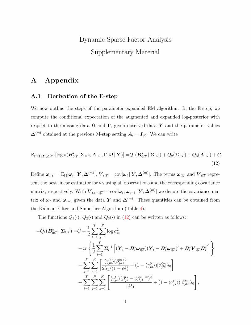
Dynamic Sparse Factor Analysis

Supplementary Material

A Appendix

A.1 Derivation of the E-step

We now outline the steps of the parameter expanded EM algorithm. In the E-step, we

compute the conditional expectation of the augmented and expanded log-posterior with

respect to the missing data Ω and Γ, given observed data Y and the parameter values

∆(m) obtained at the previous M-step setting At = IK . We can write

EΓ,Ω | Y ,∆(m) [log π(B?0:T ,Σ1:T ,A1:T ,Γ,Ω | Y )] =Q1(B?

0:T |Σ1:T ) +Q2(Σ1:T ) +Q3(A1:T ) + C.

(12)

Define ωt|T = EΩ[ωt | Y ,∆(m)], V t|T = cov[ωt | Y ,∆(m)]. The terms ωt|T and V t|T repre-

sent the best linear estimator for ωt using all observations and the corresponding covariance

matrix, respectively. With V t,t−1|T = cov[ωt,ωt−1 |Y ,∆(m)] we denote the covariance ma-

trix of ωt and ωt−1 given the data Y and ∆(m). These quantities can be obtained from

the Kalman Filter and Smoother Algorithm (Table 4).

The functions Q1(·), Q2(·) and Q3(·) in (12) can be written as follows:

−Q1(B?0:T |Σ1:T ) =C +

1

2

T∑t=1

P∑j=1

log σ2jt

+ tr

1

2

T∑t=1

Σ−1t

[(Y t −B?

tωt|T )(Y t −B?tωt|T )′ +B?

tV t|TB?′

t

]

+P∑j=1

K∑k=1

[ 〈γ0jk〉(β0∗

jk)2

2λ1/(1− φ2)+ (1− 〈γ0

jk〉)|β0∗jk |λ0

]

+T∑t=1

P∑j=1

K∑k=1

[〈γtjk〉(βt∗jk − φβt−1∗

jk )2

2λ1

+ (1− 〈γtjk〉)|βt∗jk|λ0

],

1

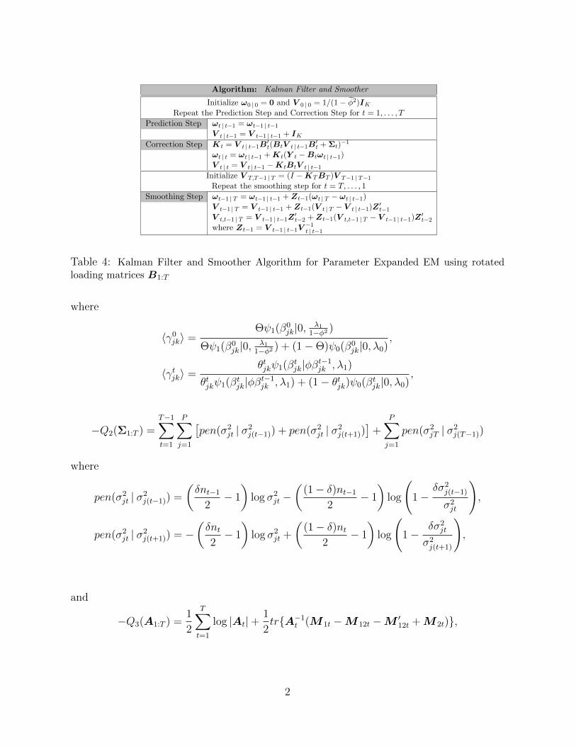
Algorithm: Kalman Filter and Smoother

Initialize ω0 | 0 = 0 and V 0 | 0 = 1/(1− φ2)IKRepeat the Prediction Step and Correction Step for t = 1, . . . , T

Prediction Step ωt | t−1 = ωt−1 | t−1

V t | t−1 = V t−1 | t−1 + IKCorrection Step Kt = V t | t−1B

′t(BtV t | t−1B

′t + Σt)

−1

ωt | t = ωt | t−1 +Kt(Y t −Btωt | t−1)

V t | t = V t | t−1 −KtBtV t | t−1

Initialize V T,T−1 | T = (I −KTBT )V T−1 | T−1

Repeat the smoothing step for t = T, . . . , 1

Smoothing Step ωt−1 | T = ωt−1 | t−1 +Zt−1(ωt | T − ωt | t−1)

V t−1 | T = V t−1 | t−1 +Zt−1(V t | T − V t | t−1)Z ′t−1

V t,t−1 | T = V t−1 | t−1Z′t−2 +Zt−1(V t,t−1 | T − V t−1 | t−1)Z ′t−2

where Zt−1 = V t−1 | t−1V−1t | t−1

Table 4: Kalman Filter and Smoother Algorithm for Parameter Expanded EM using rotatedloading matrices B1:T

where

〈γ0jk〉 =

Θψ1(β0jk|0, λ1

1−φ2 )

Θψ1(β0jk|0, λ1

1−φ2 ) + (1−Θ)ψ0(β0jk|0, λ0)

,

〈γtjk〉 =θtjkψ1(βtjk|φβt−1

jk , λ1)

θtjkψ1(βtjk|φβt−1jk , λ1) + (1− θtjk)ψ0(βtjk|0, λ0)

,

−Q2(Σ1:T ) =T−1∑t=1

P∑j=1

[pen(σ2

jt | σ2j(t−1)) + pen(σ2

jt | σ2j(t+1))

]+

P∑j=1

pen(σ2jT | σ2

j(T−1))

where

pen(σ2jt | σ2

j(t−1)) =

(δnt−1

2− 1

)log σ2

jt −(

(1− δ)nt−1

2− 1

)log

(1−

δσ2j(t−1)

σ2jt

),

pen(σ2jt | σ2

j(t+1)) = −(δnt2− 1

)log σ2

jt +

((1− δ)nt

2− 1

)log

(1−

δσ2jt

σ2j(t+1)

),

and

−Q3(A1:T ) =1

2

T∑t=1

log |At|+1

2trA−1

t (M 1t −M 12t −M ′12t +M 2t),

2

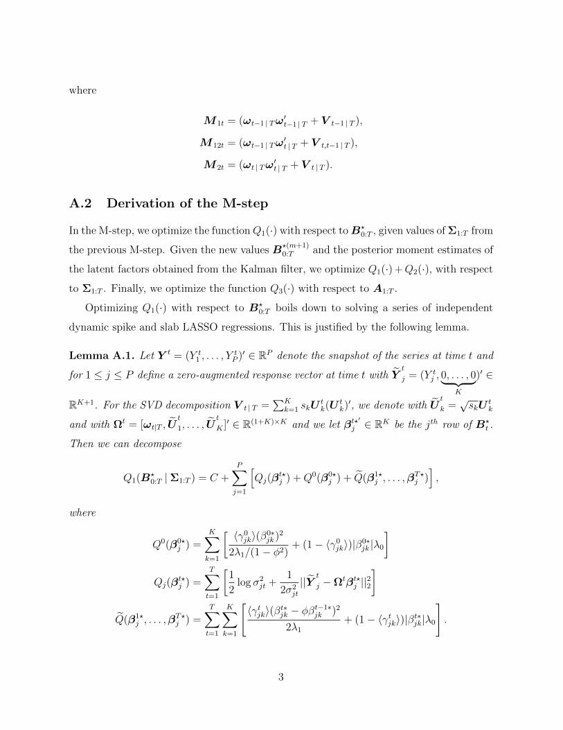
where

M 1t = (ωt−1 | Tω′t−1 | T + V t−1 | T ),

M 12t = (ωt−1 | Tω′t | T + V t,t−1 | T ),

M 2t = (ωt | Tω′t | T + V t | T ).

A.2 Derivation of the M-step

In the M-step, we optimize the functionQ1(·) with respect toB?0:T , given values of Σ1:T from

the previous M-step. Given the new values B?(m+1)0:T and the posterior moment estimates of

the latent factors obtained from the Kalman filter, we optimize Q1(·) +Q2(·), with respect

to Σ1:T . Finally, we optimize the function Q3(·) with respect to A1:T .

Optimizing Q1(·) with respect to B?0:T boils down to solving a series of independent

dynamic spike and slab LASSO regressions. This is justified by the following lemma.

Lemma A.1. Let Y t = (Y t1 , . . . , Y

tP )′ ∈ RP denote the snapshot of the series at time t and

for 1 ≤ j ≤ P define a zero-augmented response vector at time t with Yt

j = (Y tj , 0, . . . , 0︸ ︷︷ ︸

K

)′ ∈

RK+1. For the SVD decomposition V t | T =∑K

k=1 skUtk(U

tk)′, we denote with U

t

k =√skU

tk

and with Ωt = [ωt|T , Ut

1, . . . , Ut

K ]′ ∈ R(1+K)×K and we let βt?′

j ∈ RK be the jth row of B?t .

Then we can decompose

Q1(B?0:T |Σ1:T ) = C +

P∑j=1

[Qj(β

t?j ) +Q0(β0?

j ) + Q(β1?j , . . . ,β

T?j )],

where

Q0(β0?j ) =

K∑k=1

[ 〈γ0jk〉(β0∗

jk)2

2λ1/(1− φ2)+ (1− 〈γ0

jk〉)|β0∗jk |λ0

]

Qj(βt?j ) =

T∑t=1

[1

2log σ2

jt +1

2σ2jt

||Yt

j −Ωtβt?j ||22]

Q(β1?j , . . . ,β

T?j ) =

T∑t=1

K∑k=1

[〈γtjk〉(βt∗jk − φβt−1∗

jk )2

2λ1

+ (1− 〈γtjk〉)|βt∗jk|λ0

].

3

Proof. Denote with

L ≡ tr

1

2

T∑t=1

Σ−1t

[(Y t −B?

tωt|T )(Y t −B?tωt|T )′ +B?

tV t|TB?′

t

].

Because B?tV t | TB

?′

t = B?t

∑Kk=1 skU

tkU

t′

k (B?t )′ =∑K

k=1(0−B?t U

t

k)(0−B?t U

t

k)′, we have

tr

Σ−1t B

?tV t | TB

?′

t

=

K∑k=1

(0−B?t U

t

k)′Σ−1

t (0−B?t U

t

k).

Since Σt = diag(σ21t, . . . , σ

2Pt), we have

L =1

2

P∑j=1

T∑t=1

[(Y t

j − ω′t | Tβt?j )2

σ2jt

+K∑k=1

(0− Ut′kβ

t?j )2

σ2jt

]

=P∑j=1

T∑t=1

1

2σ2jt

||Yt

j −Ωtβt?j ||22.

Each summand Qj(βt?j )+Q0(β0?

j )+Q(β1?j , . . . ,β

T?j ) corresponds to a penalized dynamic

regression with K + 1 observations at each time t. Given Σt, finding B?(m+1) thereby

reduces to solving these J individual regressions. As shown in Rockova et al. (2020), each

regression can be decomposed into a sequence of univariate optimization problems. We

use the one-step late EM variant in Rockova et al. (2020) to obtain closed form one-site

updates for each β?tjk for (j, k, t). Note that this corresponds to a generalized EM, which is

aimed at improving the objective relative to the last iteration (not necessarily maximizing

it).

These univariate updates are slightly different from Rockova et al. (2020), because we

now have K + 1 observations at time t, not just one. Denote with β∗tjl the most recent

update of the coefficient β?tjl . Let

ztjk =1

σ2jt

K+1∑r=1

(Y tjr −

∑l 6=k

ωtrlβt∗jl )ω

trk

and denote

Ztjk = ztjk +

〈γtjk〉φ1

λ1

βt−1jk +

〈γt+1jk 〉φ1

λ1

βt+1jk

and

W tjk =

1

σ2jt

K+1∑r=1

(ωtrk)2 +〈γtjk〉λ1

+〈γt+1jk 〉φ2

1

λ1

.

4

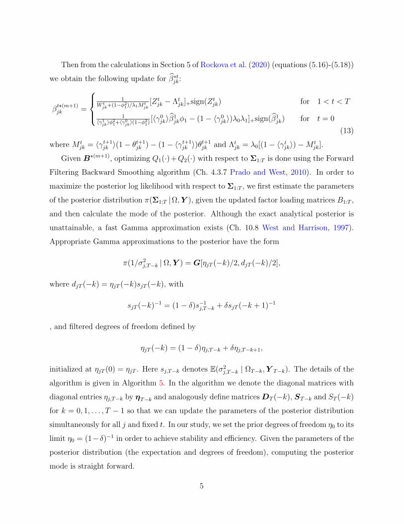
Then from the calculations in Section 5 of Rockova et al. (2020) (equations (5.16)-(5.18))

we obtain the following update for β∗tjk:

βt?(m+1)jk =

1

W tjk+(1−φ21)/λ1Mt

jk[Zt

jk − Λtjk]+sign(Zt

jk) for 1 < t < T

1〈γ1jk〉φ

21+〈γ0jk〉(1−φ

21)

[〈γ0jk〉β1

jkφ1 − (1− 〈γ0jk〉)λ0λ1]+sign(β1

jk) for t = 0

(13)

where M tjk = 〈γt+1

jk 〉(1− θt+1jk )− (1− 〈γt+1

jk 〉)θt+1jk and Λt

jk = λ0[(1− 〈γtjk〉)−M tjk].

Given B?(m+1), optimizing Q1(·)+Q2(·) with respect to Σ1:T is done using the Forward

Filtering Backward Smoothing algorithm (Ch. 4.3.7 Prado and West, 2010). In order to

maximize the posterior log likelihood with respect to Σ1:T , we first estimate the parameters

of the posterior distribution π(Σ1:T |Ω,Y ), given the updated factor loading matrices B1:T ,

and then calculate the mode of the posterior. Although the exact analytical posterior is

unattainable, a fast Gamma approximation exists (Ch. 10.8 West and Harrison, 1997).

Appropriate Gamma approximations to the posterior have the form

π(1/σ2j,T−k | Ω,Y ) = G[ηjT (−k)/2, djT (−k)/2],

where djT (−k) = ηjT (−k)sjT (−k), with

sjT (−k)−1 = (1− δ)s−1j,T−k + δsjT (−k + 1)−1

, and filtered degrees of freedom defined by

ηjT (−k) = (1− δ)ηj,T−k + δηj,T−k+1,

initialized at ηjT (0) = ηjT . Here sj,T−k denotes E(σ2j,T−k | ΩT−k,Y T−k). The details of the

algorithm is given in Algorithm 5. In the algorithm we denote the diagonal matrices with

diagonal entries ηj,T−k by ηT−k and analogously define matricesDT (−k), ST−k and ST (−k)

for k = 0, 1, . . . , T − 1 so that we can update the parameters of the posterior distribution

simultaneously for all j and fixed t. In our study, we set the prior degrees of freedom η0 to its

limit η0 = (1−δ)−1 in order to achieve stability and efficiency. Given the parameters of the

posterior distribution (the expectation and degrees of freedom), computing the posterior

mode is straight forward.

5

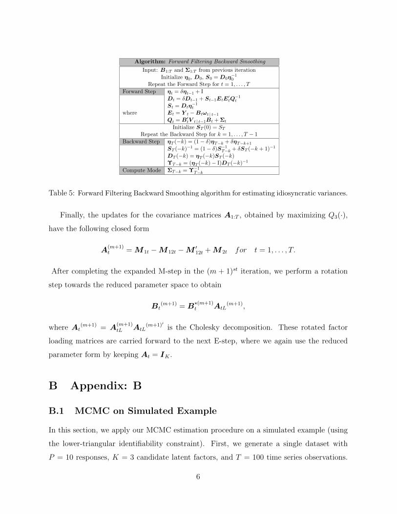
Algorithm: Forward Filtering Backward Smoothing

Input: B1:T and Σ1:T from previous iteration

Initialize η0, D0, S0 = D0η−10

Repeat the Forward Step for t = 1, . . . , T

Forward Step ηt = δηt−1 + I

Dt = δDt−1 + St−1EtE′tQ−1t

St = Dtη−1t

where Et = Y t −Btωt | t−1

Qt = B′tV t | t−1Bt + Σt

Initialize ST (0) = STRepeat the Backward Step for k = 1, . . . , T − 1

Backward Step ηT (−k) = (1− δ)ηT−k + δηT−k+1

ST (−k)−1 = (1− δ)S−1T−k + δST (−k + 1)−1

DT (−k) = ηT (−k)ST (−k)ΥT−k = (ηT (−k)− I)DT (−k)−1

Compute Mode ΣT−k = Υ−1T−k

Table 5: Forward Filtering Backward Smoothing algorithm for estimating idiosyncratic variances.

Finally, the updates for the covariance matrices A1:T , obtained by maximizing Q3(·),

have the following closed form

A(m+1)t = M 1t −M 12t −M ′

12t +M 2t for t = 1, . . . , T.

After completing the expanded M-step in the (m + 1)st iteration, we perform a rotation

step towards the reduced parameter space to obtain

Bt(m+1) = B

?(m+1)t AtL

(m+1),

where At(m+1) = A

(m+1)tL AtL

(m+1)′ is the Cholesky decomposition. These rotated factor

loading matrices are carried forward to the next E-step, where we again use the reduced

parameter form by keeping At = IK .

B Appendix: B

B.1 MCMC on Simulated Example

In this section, we apply our MCMC estimation procedure on a simulated example (using

the lower-triangular identifiability constraint). First, we generate a single dataset with

P = 10 responses, K = 3 candidate latent factors, and T = 100 time series observations.

6

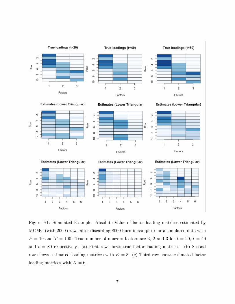
Figure B1: Simulated Example: Absolute Value of factor loading matrices estimated by

MCMC (with 2000 draws after discarding 8000 burn-in samples) for a simulated data with

P = 10 and T = 100. True number of nonzero factors are 3, 2 and 3 for t = 20, t = 40

and t = 80 respectively. (a) First row shows true factor loading matrices. (b) Second

row shows estimated loading matrices with K = 3. (c) Third row shows estimated factor

loading matrices with K = 6.

7

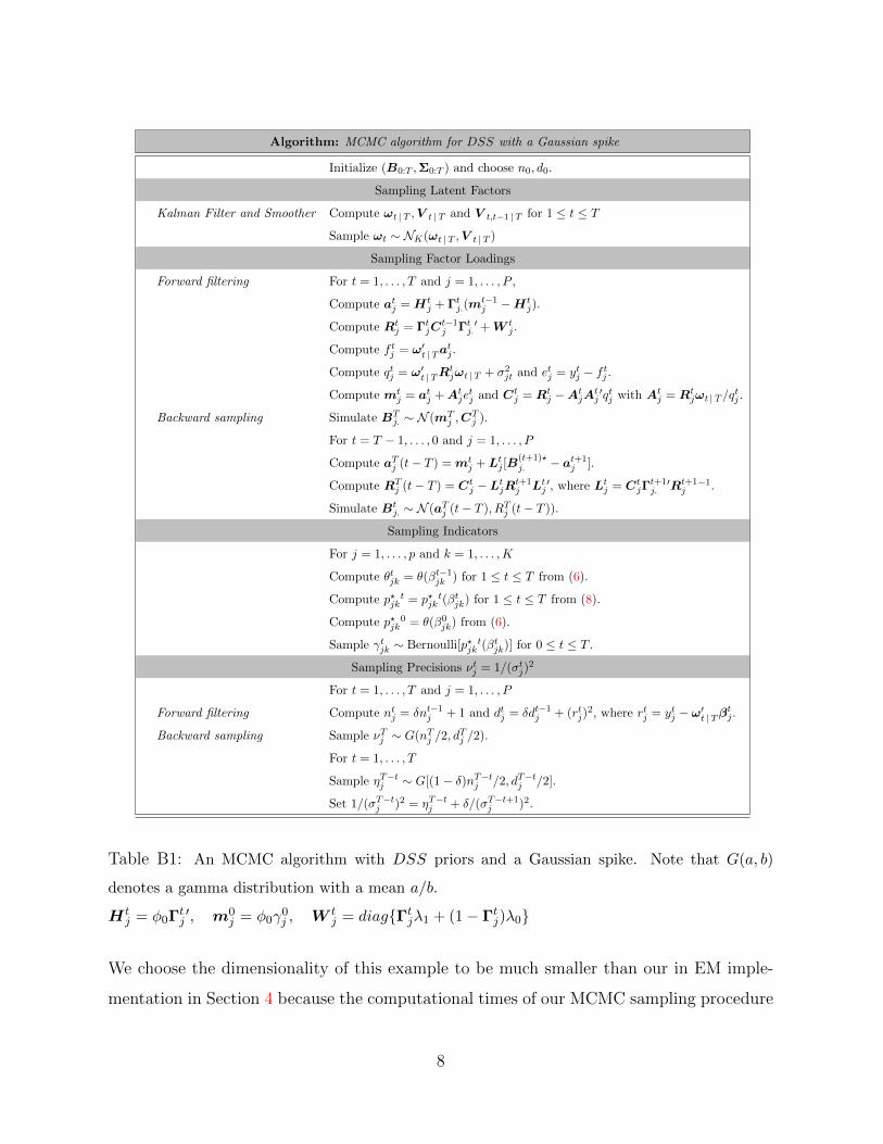
Algorithm: MCMC algorithm for DSS with a Gaussian spike

Initialize (B0:T ,Σ0:T ) and choose n0, d0.

Sampling Latent Factors

Kalman Filter and Smoother Compute ωt | T ,V t | T and V t,t−1 | T for 1 ≤ t ≤ T

Sample ωt ∼ NK(ωt | T ,V t | T )

Sampling Factor Loadings

Forward filtering For t = 1, . . . , T and j = 1, . . . , P ,

Compute atj = Htj + Γtj.(m

t−1j −Ht

j).

Compute Rtj = ΓtjC

t−1j Γtj.

′ +W tj .

Compute f tj = ω′t | Tatj .

Compute qtj = ω′t | TRtjωt | T + σ2

jt and etj = ytj − f tj .

Compute mtj = atj +At

jetj and Ct

j = Rtj −At

jAtj′qtj with At

j = Rtjωt | T /q

tj .

Backward sampling Simulate BTj. ∼ N (mT

j ,CTj ).

For t = T − 1, . . . , 0 and j = 1, . . . , P

Compute aTj (t− T ) = mtj +Ltj [B

(t+1)?j. − at+1

j ].

Compute RTj (t− T ) = Ct

j −LtjRt+1j Ltj

′, where Ltj = CtjΓ

t+1j.′Rt+1

j−1.

Simulate Btj. ∼ N (aTj (t− T ), RTj (t− T )).

Sampling Indicators

For j = 1, . . . , p and k = 1, . . . ,K

Compute θtjk = θ(βt−1jk ) for 1 ≤ t ≤ T from (6).

Compute p?jkt = p?jk

t(βtjk) for 1 ≤ t ≤ T from (8).

Compute p?jk0 = θ(β0

jk) from (6).

Sample γtjk ∼ Bernoulli[p?jkt(βtjk)] for 0 ≤ t ≤ T .

Sampling Precisions νtj = 1/(σtj)2

For t = 1, . . . , T and j = 1, . . . , P

Forward filtering Compute ntj = δnt−1j + 1 and dtj = δdt−1

j + (rtj)2, where rtj = ytj − ω′t | Tβ

tj .

Backward sampling Sample νTj ∼ G(nTj /2, dTj /2).

For t = 1, . . . , T

Sample ηT−tj ∼ G[(1− δ)nT−tj /2, dT−tj /2].

Set 1/(σT−tj )2 = ηT−tj + δ/(σT−t+1j )2.

Table B1: An MCMC algorithm with DSS priors and a Gaussian spike. Note that G(a, b)

denotes a gamma distribution with a mean a/b.

Htj = φ0Γ

tj′, m0

j = φ0γ0j , W t

j = diagΓtjλ1 + (1− Γtj)λ0

We choose the dimensionality of this example to be much smaller than our in EM imple-

mentation in Section 4 because the computational times of our MCMC sampling procedure

8

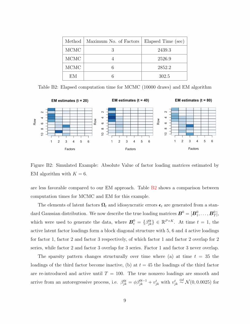
Method Maximum No. of Factors Elapsed Time (sec)

MCMC 3 2439.3

MCMC 4 2526.9

MCMC 6 2852.2

EM 6 302.5

Table B2: Elapsed computation time for MCMC (10000 draws) and EM algorithm

Figure B2: Simulated Example: Absolute Value of factor loading matrices estimated by

EM algorithm with K = 6.

are less favorable compared to our EM approach. Table B2 shows a comparison between

computation times for MCMC and EM for this example.

The elements of latent factors Ωt and idiosyncratic errors εt are generated from a stan-

dard Gaussian distribution. We now describe the true loading matricesB0 = [B01, . . . ,B

0T ],

which were used to generate the data, where B0t = β0t

jk ∈ RP×K . At time t = 1, the

active latent factor loadings form a block diagonal structure with 5, 6 and 4 active loadings

for factor 1, factor 2 and factor 3 respectively, of which factor 1 and factor 2 overlap for 2

series, while factor 2 and factor 3 overlap for 3 series. Factor 1 and factor 3 never overlap.

The sparsity pattern changes structurally over time where (a) at time t = 35 the

loadings of the third factor become inactive, (b) at t = 45 the loadings of the third factor

are re-introduced and active until T = 100. The true nonzero loadings are smooth and

arrive from an autoregressive process, i.e. β0tjk = φβ0t−1

jk + vtjk with vtjkiid∼ N (0, 0.0025) for

9

φ = 0.99, initiated at β01jk

iid∼ N (2, 1) for all 1 ≤ j ≤ P and 1 ≤ k ≤ 5. When loadings β0tjk

become inactive, they are thresholded to zero. The true factor loadings are thereby smooth

until they suddenly drop out and can re-emerge.

Figure B2 shows a heatmap of the (absolute values of) true and estimated factor load-

ings. Row 1 shows the true factor loading matrices for times t = 20, t = 40 and t = 80

respectively. Row 2 and 3 show estimated factor loadings when upper limit of latent factors

are set to K = 3 and K = 6 respectively. Posterior mean estimates of factor loadings are

obtained from an MCMC sample of size 2000, after discarding 8000 burn-in samples. We

see that for K = 6, MCMC is not able to identify actual number of factors due to factor

splitting. However estimated loading structures are close to the true loadings for K = 3.

10

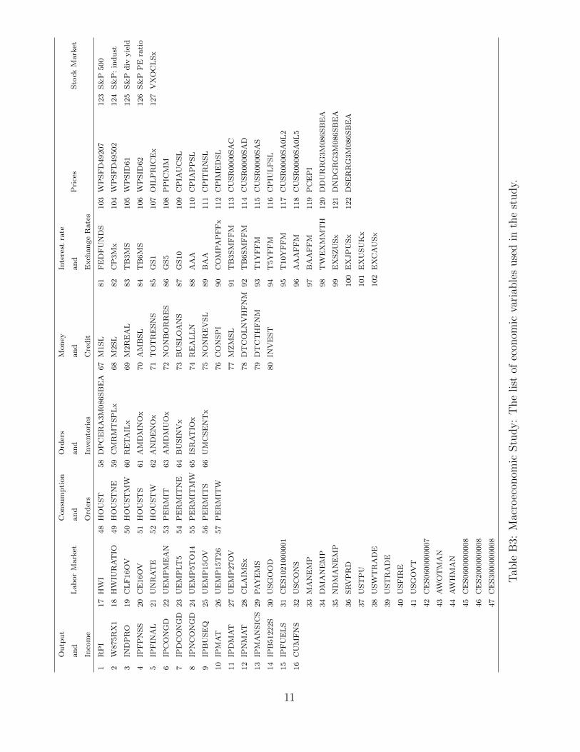
Ou

tpu

t

an

d

Inco

me

Lab

or

Mark

et

Con

sum

pti

on

an

d

Ord

ers

Ord

ers

an

d

Inven

tori

es

Mon

ey

an

d

Cre

dit

Inte

rest

rate

an

d

Exch

an

ge

Rate

s

Pri

ces

Sto

ckM

ark

et

1R

PI

17

HW

I48

HO

US

T58

DP

CE

RA

3M

086S

BE

A67

M1S

L81

FE

DF

UN

DS

103

WP

SF

D49207

123

S&

P500

2W

875R

X1

18

HW

IUR

AT

IO49

HO

US

TN

E59

CM

RM

TS

PL

x68

M2S

L82

CP

3M

x104

WP

SF

D49502

124

S&

P:

ind

ust

3IN

DP

RO

19

CL

F16O

V50

HO

US

TM

W60

RE

TA

ILx

69

M2R

EA

L83

TB

3M

S105

WP

SID

61

125

S&

Pd

ivyie

ld

4IP

FP

NS

S20

CE

16O

V51

HO

US

TS

61

AM

DM

NO

x70

AM

BS

L84

TB

6M

S106

WP

SID

62

126

S&

PP

Era

tio

5IP

FIN

AL

21

UN

RA

TE

52

HO

US

TW

62

AN

DE

NO

x71

TO

TR

ES

NS

85

GS

1107

OIL

PR

ICE

x127

VX

OC

LS

x

6IP

CO

NG

D22

UE

MP

ME

AN

53

PE

RM

IT63

AM

DM

UO

x72

NO

NB

OR

RE

S86

GS

5108

PP

ICM

M

7IP

DC

ON

GD

23

UE

MP

LT

554

PE

RM

ITN

E64

BU

SIN

Vx

73

BU

SL

OA

NS

87

GS

10

109

CP

IAU

CS

L

8IP

NC

ON

GD

24

UE

MP

5T

O14

55

PE

RM

ITM

W65

ISR

AT

IOx

74

RE

AL

LN

88

AA

A110

CP

IAP

PS

L

9IP

BU

SE

Q25

UE

MP

15O

V56

PE

RM

ITS

66

UM

CS

EN

Tx

75

NO

NR

EV

SL

89

BA

A111

CP

ITR

NS

L

10

IPM

AT

26

UE

MP

15T

26

57

PE

RM

ITW

76

CO

NS

PI

90

CO

MP

AP

FF

x112

CP

IME

DS

L

11

IPD

MA

T27

UE

MP

27O

V77

MZ

MS

L91

TB

3S

MF

FM

113

CU

SR

0000S

AC

12

IPN

MA

T28

CL

AIM

Sx

78

DT

CO

LN

VH

FN

M92

TB

6S

MF

FM

114

CU

SR

0000S

AD

13

IPM

AN

SIC

S29

PA

YE

MS

79

DT

CT

HF

NM

93

T1Y

FF

M115

CU

SR

0000S

AS

14

IPB

51222S

30

US

GO

OD

80

INV

ES

T94

T5Y

FF

M116

CP

IUL

FS

L

15

IPF

UE

LS

31

CE

S1021000001

95

T10Y

FF

M117

CU

SR

0000S

A0L

2

16

CU

MF

NS

32

US

CO

NS

96

AA

AF

FM

118

CU

SR

0000S

A0L

5

33

MA

NE

MP

97

BA

AF

FM

119

PC

EP

I

34

DM

AN

EM

P98

TW

EX

MM

TH

120

DD

UR

RG

3M

086S

BE

A

35

ND

MA

NE

MP

99

EX

SZ

US

x121

DN

DG

RG

3M

086S

BE

A

36

SR

VP

RD

100

EX

JP

US

x122

DS

ER

RG

3M

086S

BE

A

37

US

TP

U101

EX

US

UK

x

38

US

WT

RA

DE

102

EX

CA

US

x

39

US

TR

AD

E

40

US

FIR

E

41

US

GO

VT

42

CE

S0600000007

43

AW

OT

MA

N

44

AW

HM

AN

45

CE

S0600000008

46

CE

S2000000008

47

CE

S3000000008

Tab

leB

3:M

acro

econ

omic

Stu

dy:

The

list

ofec

onom

icva

riab

les

use

din

the

study.

11