A Kronecker-factored approximate Fisher matrix for convolution layers

A Kronecker-factored approximate Fisher matrix for convolution layers

Roger Grosse [email protected] Martens [email protected]

Department of Computer Science, University of Toronto

AbstractSecond-order optimization methods such as nat-ural gradient descent have the potential to speedup training of neural networks by correcting forthe curvature of the loss function. Unfortunately,the exact natural gradient is impractical to com-pute for large models, and most approximationseither require an expensive iterative procedureor make crude approximations to the curvature.We present Kronecker Factors for Convolution(KFC), a tractable approximation to the Fishermatrix for convolutional networks based on astructured probabilistic model for the distributionover backpropagated derivatives. Similarly to therecently proposed Kronecker-Factored Approxi-mate Curvature (K-FAC), each block of the ap-proximate Fisher matrix decomposes as the Kro-necker product of small matrices, allowing for ef-ficient inversion. KFC captures important curva-ture information while still yielding comparablyefficient updates to stochastic gradient descent(SGD). We show that the updates are invariantto commonly used reparameterizations, such ascentering of the activations. In our experiments,approximate natural gradient descent with KFCwas able to train convolutional networks severaltimes faster than carefully tuned SGD. Further-more, it was able to train the networks in 10-20times fewer iterations than SGD, suggesting itspotential applicability in a distributed setting.

1. IntroductionDespite advances in optimization, most neural networks arestill trained using variants of stochastic gradient descent(SGD) with momentum. It has been suggested that natu-ral gradient descent (Amari, 1998) could greatly speed upoptimization because it accounts for the geometry of theoptimization landscape and has desirable invariance prop-erties. (See Martens (2014) for a review.) Unfortunately,

Proceedings of the 33 rd International Conference on MachineLearning, New York, NY, USA, 2016. JMLR: W&CP volume48. Copyright 2016 by the author(s).

computing the exact natural gradient is intractable for largenetworks, as it requires solving a large linear system in-volving the Fisher matrix, whose dimension is the numberof parameters (potentially tens of millions for modern ar-chitectures). Approximations to the natural gradient typi-cally either impose very restrictive structure on the Fishermatrix (e.g. LeCun et al., 1998; Le Roux et al., 2008) orrequire expensive iterative procedures to compute each up-date, analogously to approximate Newton methods (e.g.Martens, 2010). An ongoing challenge has been to developa curvature matrix approximation which reflects enoughstructure to yield high-quality updates, while introducingminimal computational overhead beyond the standard gra-dient computations.

Much progress in machine learning has been driven bythe development of structured probabilistic models whoseindependence structure allows for efficient computations,yet which still capture important dependencies between thevariables of interest. In our case, since the Fisher ma-trix is the covariance of the backpropagated log-likelihoodderivatives, we are interested in modeling the distributionover these derivatives. The model must support efficientcomputation of the inverse covariance, as this is what’srequired to compute the natural gradient. Recently, theFactorized Natural Gradient (FANG) (Grosse & Salakhut-dinov, 2015) and Kronecker-Factored Approximate Cur-vature (K-FAC) (Martens & Grosse, 2015) methods ex-ploited probabilistic models of the derivatives to efficientlycompute approximate natural gradient updates. In its sim-plest version, K-FAC approximates each layer-wise blockof the Fisher matrix as the Kronecker product of two muchsmaller matrices. These (very large) blocks can then becan be tractably inverted by inverting each of the two fac-tors. K-FAC was shown to greatly speed up the training ofdeep autoencoders. However, its underlying probabilisticmodel assumed fully connected networks with no weightsharing, rendering the method inapplicable to two archi-tectures which have recently revolutionized many applica-tions of machine learning — convolutional networks (Le-Cun et al., 1989; Krizhevsky et al., 2012) and recurrent neu-ral networks (Hochreiter & Schmidhuber, 1997; Sutskeveret al., 2014).

We introduce Kronecker Factors for Convolution (KFC), anapproximation to the Fisher matrix for convolutional net-


works. Most modern convolutional networks have trainableparameters only in convolutional and fully connected lay-ers. Standard K-FAC can be applied to the latter; our contri-bution is a factorization of the Fisher blocks correspondingto convolution layers. KFC is based on a structured proba-bilistic model of the backpropagated derivatives where theactivations are independent of the derivatives, the activa-tions and derivatives are spatially homogeneous, and thederivatives are spatially uncorrelated. Under these approx-imations, we show that the Fisher blocks for convolutionlayers decompose as a Kronecker product of smaller matri-ces (analogously to K-FAC), yielding tractable updates.

KFC yields a tractable approximation to the Fisher matrixof a conv net. It can be used directly to compute approxi-mate natural gradient descent updates, as we do in our ex-periments. One could further combine it with the adap-tive step size, momentum, and damping methods from thefull K-FAC algorithm (Martens & Grosse, 2015). It couldalso potentially be used as a pre-conditioner for iterativesecond-order methods (Martens, 2010; Vinyals & Povey,2012; Sohl-Dickstein et al., 2014). We show that the ap-proximate natural gradient updates are invariant to widelyused reparameterizations of a network, such as whiteningor centering of the activations.

We have evaluated our method on training conv nets on ob-ject recognition benchmarks. In our experiments, KFC wasable to optimize conv nets several times faster than care-fully tuned SGD with momentum, in terms of both trainingand test error. Furthermore, it required 10-20 times feweriterations, suggesting its usefulness in the context of highlydistributed training algorithms.

2. BackgroundIn this section, we outline the K-FAC method as previouslyformulated for standard fully-connected feed-forward net-works without weight sharing (Martens & Grosse, 2015).Each layer of a fully connected network computes activa-tions as:

s` = W`¯a`�1 (1)a` = �`(s`), (2)

where ` 2 {1, . . . , L} indexes the layer, s` denotes theinputs to the layer, a` denotes the activations, ¯

W` =

(b` W`) denotes the matrix of biases and weights, ¯a` =

(1 a

>` )

> denotes the activations with a homogeneous di-mension appended, and �` denotes a nonlinear activationfunction (usually applied coordinate-wise). (Throughoutthis paper, we will use the index 0 for all homogeneous co-ordinates.) We will refer to the values s` as pre-activations.By convention, a0 corresponds to the inputs x and aL cor-responds to the prediction z made by the network. For con-venience, we concatenate all of the parameters of the net-work into a vector ✓ = (vec(W1)

>, . . . , vec(WL)>)

>,where vec denotes the Kronecker vector operator whichstacks the columns of a matrix into a vector. We denote

the function computed by the network as f(x,✓) = aL.

Typically, a network is trained to minimize an objectiveh(✓) given by L(y, f(x,✓)) as averaged over the trainingset, where L(y, z) is a loss function. The gradient rh ofh(✓), which is required by most optimization methods, isestimated stochastically using mini-batches of training ex-amples. (We will often drop the explicit ✓ subscript whenthe meaning is unambiguous.)

For the remainder of this paper, we will assume the net-work’s prediction f(x,✓) determines the value of the pa-rameter z of a distribution R

y|z over y, and the loss func-tion is the corresponding negative log-likelihood L(y, z) =� log r(y|z).

2.1. Second-order optimization of neural networks

Second-order optimization methods work by computing aparameter update v that minimizes (or approximately min-imizes) a local quadratic approximation to the objective,given by h(✓) = r✓h>

v +

12v

>Cv, where C is a ma-

trix which quantifies the curvature of the cost function hat ✓. The exact solution to this minimization problem canbe obtained by solving the linear system Cv = �r✓h.The original and most well-known example is Newton’smethod, where C is chosen to be the Hessian matrix;this isn’t appropriate in the non-convex setting because ofthe well-known problem that it searches for critical pointsrather than local optima (e.g. Pascanu et al., 2014). There-fore, it is more common to use natural gradient (Amari,1998) or updates based on the generalized Gauss-Newtonmatrix (Schraudolph, 2002), which are guaranteed to pro-duce descent directions because the curvature matrix C ispositive semidefinite.

Natural gradient descent can be usefully interpreted asa second-order method (Martens, 2014) where C is theFisher information matrix F, as given by

F = E x⇠pdatay⇠R

y|f(x,✓)

⇥D✓(D✓)>

⇤, (3)

where pdata denotes the training distribution, Ry|f(x,✓)

denotes the model’s predictive distribution, and D✓ =

r✓L(y, f(x,✓)) is the log-likelihood gradient. For the re-mainder of this paper, all expectations are with respect tothis distribution (which we term the model’s distribution),so we will leave off the subscripts. (In this paper, we willuse the D notation for log-likelihood derivatives; deriva-tives of other functions will be written out explicitly.) Inthe case where R

y|z corresponds to an exponential familymodel with “natural” parameters given by z, F is equiv-alent to the generalized Gauss-Newton matrix (Martens,2014), which is an approximation of the Hessian which hasalso seen extensive use in various neural-network optimiza-tion methods (e.g. Martens, 2010; Vinyals & Povey, 2012).

F is an n ⇥ n matrix, where n is the number of param-eters and can be in the tens of millions for modern deeparchitectures. Therefore, it is impractical to represent F


explicitly in memory, let alone solve the linear system ex-actly. There are two general strategies one typically takesto find a good search direction: either impose a structure onF enabling fast inversion (e.g. LeCun et al., 1998; Le Rouxet al., 2008; Grosse & Salakhutdinov, 2015), or use an it-erative procedure to approximately solve the linear system(e.g. Martens, 2010). These two strategies are not mutu-ally exclusive: tractable curvature approximations can beused as preconditioners in second order optimization, andthis has been observed to make a large difference (Martens,2010; Chapelle & Erhan, 2011; Vinyals & Povey, 2012).

2.2. Kronecker-factored approximate curvature

Kronecker-factored approximate curvature (K-FAC;Martens & Grosse, 2015) is a recently proposed optimiza-tion method for neural networks which can be seen asa hybrid of the two approximation strategies: it uses atractable approximation to the Fisher matrix F, but alsouses an optimization strategy which behaves locally likeconjugate gradient. This section gives a conceptual sum-mary of the aspects of K-FAC relevant to the contributionsof this paper; a precise description of the full algorithm isgiven in Appendix B.2.

The block-diagonal version of K-FAC (which is the simplerof the two versions, and is what we will present here) isbased on two approximations to F which together make ittractable to invert. First, weight derivatives in different lay-ers are assumed to be uncorrelated, which corresponds to F

being block diagonal, with one block per layer. Each blockis given by E[vec(D ¯

W`) vec(D ¯

W`)>]. This approxima-

tion by itself is insufficient, because each of the blocks maystill be very large. (E.g., if a network has 1,000 units ineach layer, each block would be of size 106⇥ 10

6.) For thesecond approximation, observe that

E⇥D[

¯

W`]ijD[

¯

W`]i0j0⇤= E [D[s`]i[¯a`�1]jD[s`]i0 [¯a`�1]j0 ] .

If we approximate the activations and pre-activation derivatives as independent, this canbe decomposed as E

⇥D[

¯

W`]ijD[

¯

W`]i0j0⇤

⇡E [D[s`]iD[s`]i0 ]E [[

¯

a`�1]j [¯a`�1]j0 ]. This can be writtenalgebraically as a decomposition into a Kronecker productof two smaller matrices:

E[vec( ¯W`) vec(¯

W`)>] ⇡ `�1 ⌦ �` , ˆ

F`, (4)

where `�1 = E[¯a`�1¯a>`�1] and �` = E[s`s>` ] denote

the second moment matrices of the activations and pre-activation derivatives, respectively. Call the block diagonalapproximate Fisher matrix, with blocks given by Eqn. 4,ˆ

F. The two factors are estimated online from the empiri-cal moments of the model’s distribution using exponentialmoving averages.

To invert ˆF, we use the facts that (1) we can invert a blockdiagonal matrix by inverting each of the blocks, and (2)the Kronecker product satisfies the identity (A ⌦B)

�1=

A

�1 ⌦B

�1:

ˆ

F

�1=

0

B@

�10 ⌦ ��1

1 0

. . .0

�1L�1 ⌦ �

�1L

1

CA (5)

We do not represent ˆF�1 explicitly, as each of the blocks isquite large. Instead, we keep track of each of the Kroneckerfactors.

The approximate natural gradient ˆF�1rh can then be com-puted as follows:

ˆ

F

�1rh =

0

B@vec

��

�11 (r

¯

W1h) �1

0

�

...vec

��

�1L (r

¯

WLh) �1

L�1

�

1

CA (6)

We would often like to add a multiple of the identity ma-trix to F for two reasons. First, many networks are regu-larized with weight decay, which corresponds to a penaltyof 1

2�✓>✓, for some parameter �. Following the interpre-

tation of F as a quadratic approximation to the curvature,it would be appropriate to use F + �I to approximate thecurvature of the regularized objective. The second reasonis that the local quadratic approximation of h implicitlyused when computing the natural gradient may be inaccu-rate over the region of interest, owing to the approximationof F by ˆ

F, to the approximation of the Hessian by F, andfinally to the error associated with approximating h as lo-cally quadratic in the first place. A common way to ad-dress this issue is to damp the updates by adding �I to theapproximate curvature matrix, for some small value �, be-fore minimizing the local quadratic model. Therefore, we

would ideally like to computehˆ

F+ (�+ �)Ii�1

rh.

Unfortunately, adding (� + �)I breaks the Kronecker fac-torization structure. While it is possible to exactly solve thedamped system (see Appendix B.2), it is often preferable toapproximate ˆ

F+ (�+ �)I in a way that maintains the fac-torizaton structure. Martens & Grosse (2015) pointed outthat

F`+(�+�)I ⇡⇣ `�1 + ⇡`

p�+ � I

⌘⌦✓�` +

1⇡`

p�+ � I

◆.

(7)We will denote this damped approximation as ˆ

F

(�)` =

(�)`�1⌦�

(�)` . Mathematically, ⇡` can be any positive scalar,

but Martens & Grosse (2015) suggest the formula

⇡` =

sk `�1 ⌦ IkkI⌦ �`k

, (8)

where k · k denotes some matrix norm, as this value mini-mizes the norm of the residual in Eqn. 7. In this work, weuse the trace norm kBk = trB. The approximate natural


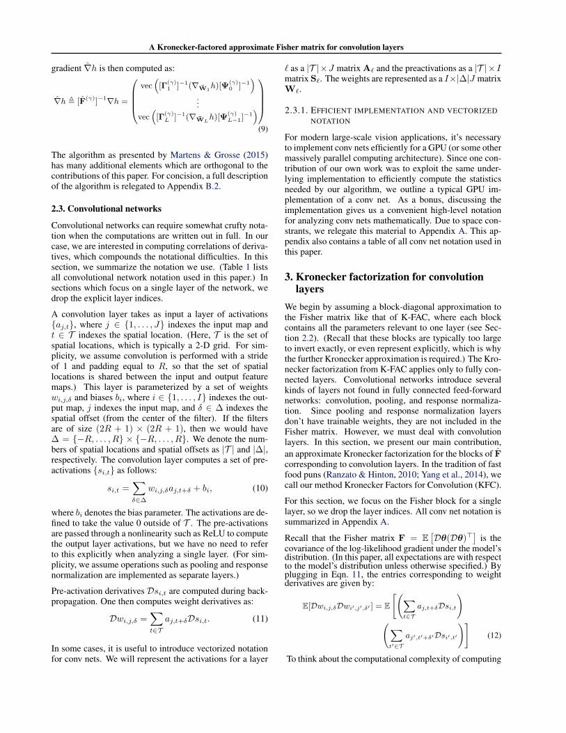
gradient ˆrh is then computed as:

rh , [F(�)]�1rh =

0

BBB@

vec⇣[�(�)

1 ]�1(rW1h)[ (�)

0 ]�1⌘

...vec⇣[�(�)

L ]�1(rWLh)[ (�)

L�1]�1⌘

1

CCCA

(9)

The algorithm as presented by Martens & Grosse (2015)has many additional elements which are orthogonal to thecontributions of this paper. For concision, a full descriptionof the algorithm is relegated to Appendix B.2.

2.3. Convolutional networks

Convolutional networks can require somewhat crufty nota-tion when the computations are written out in full. In ourcase, we are interested in computing correlations of deriva-tives, which compounds the notational difficulties. In thissection, we summarize the notation we use. (Table 1 listsall convolutional network notation used in this paper.) Insections which focus on a single layer of the network, wedrop the explicit layer indices.

A convolution layer takes as input a layer of activations{aj,t}, where j 2 {1, . . . , J} indexes the input map andt 2 T indexes the spatial location. (Here, T is the set ofspatial locations, which is typically a 2-D grid. For sim-plicity, we assume convolution is performed with a strideof 1 and padding equal to R, so that the set of spatiallocations is shared between the input and output featuremaps.) This layer is parameterized by a set of weightswi,j,� and biases bi, where i 2 {1, . . . , I} indexes the out-put map, j indexes the input map, and � 2 � indexes thespatial offset (from the center of the filter). If the filtersare of size (2R + 1) ⇥ (2R + 1), then we would have� = {�R, . . . , R} ⇥ {�R, . . . , R}. We denote the num-bers of spatial locations and spatial offsets as |T | and |�|,respectively. The convolution layer computes a set of pre-activations {si,t} as follows:

si,t =X

�2�

wi,j,�aj,t+� + bi, (10)

where bi denotes the bias parameter. The activations are de-fined to take the value 0 outside of T . The pre-activationsare passed through a nonlinearity such as ReLU to computethe output layer activations, but we have no need to referto this explicitly when analyzing a single layer. (For sim-plicity, we assume operations such as pooling and responsenormalization are implemented as separate layers.)

Pre-activation derivatives Dsi,t are computed during back-propagation. One then computes weight derivatives as:

Dwi,j,� =

X

t2Taj,t+�Dsi,t. (11)

In some cases, it is useful to introduce vectorized notationfor conv nets. We will represent the activations for a layer

` as a |T |⇥J matrix A` and the preactivations as a |T |⇥Imatrix S`. The weights are represented as a I⇥|�|J matrixW`.

2.3.1. EFFICIENT IMPLEMENTATION AND VECTORIZEDNOTATION

For modern large-scale vision applications, it’s necessaryto implement conv nets efficiently for a GPU (or some othermassively parallel computing architecture). Since one con-tribution of our own work was to exploit the same under-lying implementation to efficiently compute the statisticsneeded by our algorithm, we outline a typical GPU im-plementation of a conv net. As a bonus, discussing theimplementation gives us a convenient high-level notationfor analyzing conv nets mathematically. Due to space con-strants, we relegate this material to Appendix A. This ap-pendix also contains a table of all conv net notation used inthis paper.

3. Kronecker factorization for convolutionlayers

We begin by assuming a block-diagonal approximation tothe Fisher matrix like that of K-FAC, where each blockcontains all the parameters relevant to one layer (see Sec-tion 2.2). (Recall that these blocks are typically too largeto invert exactly, or even represent explicitly, which is whythe further Kronecker approximation is required.) The Kro-necker factorization from K-FAC applies only to fully con-nected layers. Convolutional networks introduce severalkinds of layers not found in fully connected feed-forwardnetworks: convolution, pooling, and response normaliza-tion. Since pooling and response normalization layersdon’t have trainable weights, they are not included in theFisher matrix. However, we must deal with convolutionlayers. In this section, we present our main contribution,an approximate Kronecker factorization for the blocks of ˆFcorresponding to convolution layers. In the tradition of fastfood puns (Ranzato & Hinton, 2010; Yang et al., 2014), wecall our method Kronecker Factors for Convolution (KFC).

For this section, we focus on the Fisher block for a singlelayer, so we drop the layer indices. All conv net notation issummarized in Appendix A.

Recall that the Fisher matrix F = E⇥D✓(D✓)>

⇤is the

covariance of the log-likelihood gradient under the model’sdistribution. (In this paper, all expectations are with respectto the model’s distribution unless otherwise specified.) Byplugging in Eqn. 11, the entries corresponding to weightderivatives are given by:

E[Dwi,j,�Dwi0,j0,�0 ] = E" X

t2T

aj,t+�Dsi,t

!

X

t02T

aj0,t0+�0Dsi0,t0

!#(12)

To think about the computational complexity of computing


the entries directly, consider the second convolution layerof AlexNet (Krizhevsky et al., 2012), which has 48 inputfeature maps, 128 output feature maps, 27 ⇥ 27 = 729

spatial locations, and 5 ⇥ 5 filters. Since there are 128 ⇥48⇥5⇥5 = 245760 weights and 128 biases, the full blockwould require 245888

2 ⇡ 60.5 billion entries to representexplicitly, and inversion is clearly impractical.

Recall that K-FAC approximation for classical fully con-nected networks can be derived by approximating activa-tions and pre-activation derivatives as being statistically in-dependent (this is the IAD approximation below). Derivingan analogous Fisher approximation for convolution layerswill require some additional approximations.

Here are the approximations we will make in deriving ourFisher approximation:

• Independent activations and derivatives (IAD).The activations are independent of the pre-activationderivatives, i.e. {aj,t} ?? {Dsi,t0}.

• Spatial homogeneity (SH). The first-order statisticsof the activations are independent of spatial location.The second-order statistics of the activations and pre-activation derivatives at any two spatial locations t andt0 depend only on t0 � t. This implies there are func-tions M , ⌦ and � such that:

E [aj,t] = M(j) (13)E [aj,taj0,t0 ] = ⌦(j, j0, t0 � t) (14)

E [Dsi,tDsi0,t0 ] = �(i, i0, t0 � t). (15)

Note that E[Dsi,t] = 0 under the model’s distribution,so Cov (Dsi,t,Dsi0,t0) = E [Dsi,tDsi0,t0 ].

• Spatially uncorrelated derivatives (SUD). The pre-activation derivatives at any two distinct spatial loca-tions are uncorrelated, i.e. �(i, i0, �) = 0 for � 6= 0.

We believe SH is fairly innocuous, as one is implicitly mak-ing a spatial homogeneity assumption when choosing touse convolution in the first place. SUD perhaps sounds likea more severe approximation, but in fact appeared to de-scribe the model’s distribution quite well in the networkswe investigated; this is analyzed empirially in Section 5.1.

We now show that combining the above three approx-imations yields a Kronecker factorization of the Fisherblocks. For simplicity of notation, assume the data are two-dimensional, so that the offsets can be parameterized withindices � = (�1, �2) and �0 = (�01, �

02), and denote the di-

mensions of the activations map as (T1, T2). The formulascan be generalized to data dimensions higher than 2 in theobvious way. For clarity, we leave out the bias parametersin this section, but these are discussed in Appendix E.

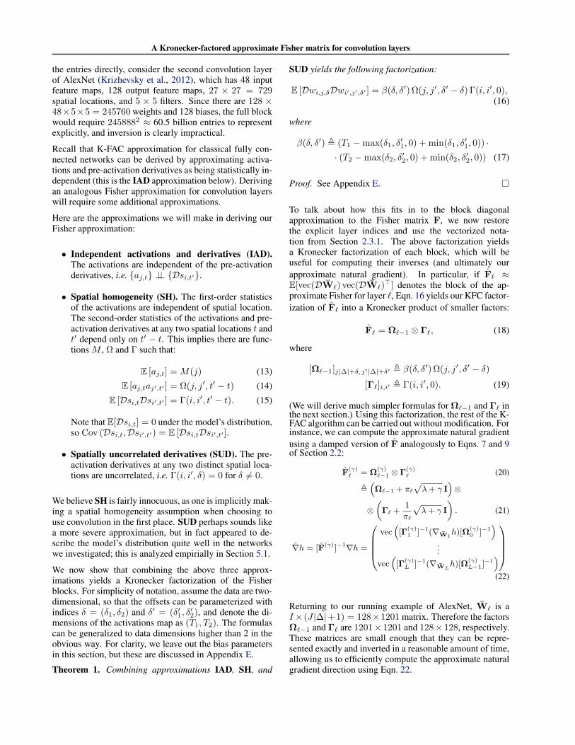
Theorem 1. Combining approximations IAD, SH, and

SUD yields the following factorization:

E [Dwi,j,�Dwi0,j0,�0 ] = �(�, �0)⌦(j, j0, �0 � �)�(i, i0, 0),(16)

where

�(�, �0) , (T1 �max(�1, �01, 0) + min(�1, �

01, 0)) ·

· (T2 �max(�2, �02, 0) + min(�2, �

02, 0)) (17)

Proof. See Appendix E.

To talk about how this fits in to the block diagonalapproximation to the Fisher matrix F, we now restorethe explicit layer indices and use the vectorized nota-tion from Section 2.3.1. The above factorization yieldsa Kronecker factorization of each block, which will beuseful for computing their inverses (and ultimately ourapproximate natural gradient). In particular, if ˆ

F` ⇡E[vec(D ¯

W`) vec(D ¯

W`)>] denotes the block of the ap-

proximate Fisher for layer `, Eqn. 16 yields our KFC factor-ization of ˆ

F` into a Kronecker product of smaller factors:

ˆ

F` = ⌦`�1 ⌦ �`, (18)

where

[⌦`�1]j|�|+�, j0|�|+�0 , �(�, �0)⌦(j, j0, �0 � �)

[�`]i,i0 , �(i, i0, 0). (19)

(We will derive much simpler formulas for ⌦`�1 and �` inthe next section.) Using this factorization, the rest of the K-FAC algorithm can be carried out without modification. Forinstance, we can compute the approximate natural gradientusing a damped version of ˆ

F analogously to Eqns. 7 and 9of Section 2.2:

F(�)` = ⌦(�)

`�1 ⌦ �(�)` (20)

,⇣⌦`�1 + ⇡`

p�+ � I

⌘⌦

⌦✓�` +

1⇡`

p�+ � I

◆. (21)

rh = [F(�)]�1rh =

0

BBB@

vec⇣[�(�)

1 ]�1(rW1h)[⌦(�)

0 ]�1⌘

...vec

⇣[�(�)

L ]�1(rWLh)[⌦(�)

L�1]�1

⌘

1

CCCA

(22)

Returning to our running example of AlexNet, ¯

W` is aI⇥ (J |�|+1) = 128⇥1201 matrix. Therefore the factors⌦`�1 and �` are 1201⇥ 1201 and 128⇥ 128, respectively.These matrices are small enough that they can be repre-sented exactly and inverted in a reasonable amount of time,allowing us to efficiently compute the approximate naturalgradient direction using Eqn. 22.


3.1. Estimating the factors

Since the true covariance statistics are unknown, we esti-mate them empirically by sampling from the model’s dis-tribution, similarly to Martens & Grosse (2015). To sam-ple derivatives from the model’s distribution, we select amini-batch, sample the outputs from the model’s predictivedistribution, and backpropagate the derivatives.

We need to estimate the Kronecker factors {⌦`}L�1`=0 and

{�`}L`=1. Since these matrices are defined in terms of theautocovariance functions ⌦ and �, it would appear natu-ral to estimate these functions empirically. Unfortunately,if the empirical autocovariances are plugged into Eqn. 19,the resulting ⌦` may not be positive semidefinite. Thisis a problem, since negative eigenvalues in the approxi-mate Fisher could cause the optimization to diverge (a phe-nomenon we have observed in practice).

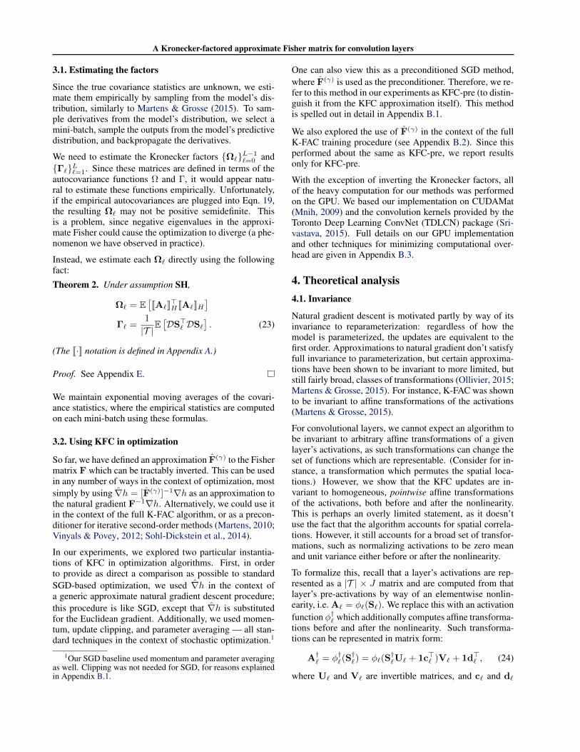
Instead, we estimate each ⌦` directly using the followingfact:Theorem 2. Under assumption SH,

⌦` = E⇥JA`K>HJA`KH

⇤

�` =1

|T |E⇥DS

>` DS`

⇤. (23)

(The J·K notation is defined in Appendix A.)


We maintain exponential moving averages of the covari-ance statistics, where the empirical statistics are computedon each mini-batch using these formulas.

3.2. Using KFC in optimization

So far, we have defined an approximation ˆ

F

(�) to the Fishermatrix F which can be tractably inverted. This can be usedin any number of ways in the context of optimization, mostsimply by using ˆrh = [

ˆ

F

(�)]

�1rh as an approximation tothe natural gradient F�1rh. Alternatively, we could use itin the context of the full K-FAC algorithm, or as a precon-ditioner for iterative second-order methods (Martens, 2010;Vinyals & Povey, 2012; Sohl-Dickstein et al., 2014).

In our experiments, we explored two particular instantia-tions of KFC in optimization algorithms. First, in orderto provide as direct a comparison as possible to standardSGD-based optimization, we used ˆrh in the context ofa generic approximate natural gradient descent procedure;this procedure is like SGD, except that ˆrh is substitutedfor the Euclidean gradient. Additionally, we used momen-tum, update clipping, and parameter averaging — all stan-dard techniques in the context of stochastic optimization.1

1Our SGD baseline used momentum and parameter averagingas well. Clipping was not needed for SGD, for reasons explainedin Appendix B.1.

One can also view this as a preconditioned SGD method,where ˆ

F

(�) is used as the preconditioner. Therefore, we re-fer to this method in our experiments as KFC-pre (to distin-guish it from the KFC approximation itself). This methodis spelled out in detail in Appendix B.1.

We also explored the use of ˆ

F

(�) in the context of the fullK-FAC training procedure (see Appendix B.2). Since thisperformed about the same as KFC-pre, we report resultsonly for KFC-pre.

With the exception of inverting the Kronecker factors, allof the heavy computation for our methods was performedon the GPU. We based our implementation on CUDAMat(Mnih, 2009) and the convolution kernels provided by theToronto Deep Learning ConvNet (TDLCN) package (Sri-vastava, 2015). Full details on our GPU implementationand other techniques for minimizing computational over-head are given in Appendix B.3.

4. Theoretical analysis4.1. Invariance

Natural gradient descent is motivated partly by way of itsinvariance to reparameterization: regardless of how themodel is parameterized, the updates are equivalent to thefirst order. Approximations to natural gradient don’t satisfyfull invariance to parameterization, but certain approxima-tions have been shown to be invariant to more limited, butstill fairly broad, classes of transformations (Ollivier, 2015;Martens & Grosse, 2015). For instance, K-FAC was shownto be invariant to affine transformations of the activations(Martens & Grosse, 2015).

For convolutional layers, we cannot expect an algorithm tobe invariant to arbitrary affine transformations of a givenlayer’s activations, as such transformations can change theset of functions which are representable. (Consider for in-stance, a transformation which permutes the spatial loca-tions.) However, we show that the KFC updates are in-variant to homogeneous, pointwise affine transformationsof the activations, both before and after the nonlinearity.This is perhaps an overly limited statement, as it doesn’tuse the fact that the algorithm accounts for spatial correla-tions. However, it still accounts for a broad set of transfor-mations, such as normalizing activations to be zero meanand unit variance either before or after the nonlinearity.

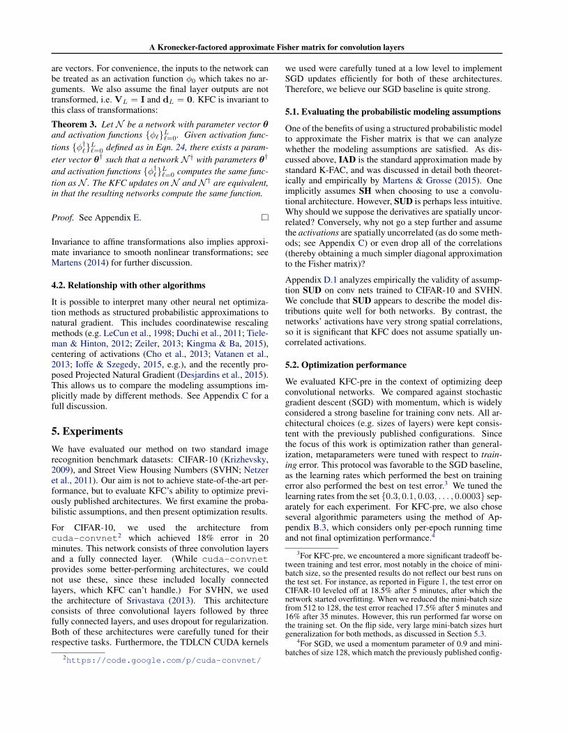
To formalize this, recall that a layer’s activations are rep-resented as a |T | ⇥ J matrix and are computed from thatlayer’s pre-activations by way of an elementwise nonlin-earity, i.e. A` = �`(S`). We replace this with an activationfunction �†

` which additionally computes affine transforma-tions before and after the nonlinearity. Such transforma-tions can be represented in matrix form:

A

†` = �†

`(S†`) = �`(S

†`U` + 1c

>` )V` + 1d

>` , (24)

where U` and V` are invertible matrices, and c` and d`


are vectors. For convenience, the inputs to the network canbe treated as an activation function �0 which takes no ar-guments. We also assume the final layer outputs are nottransformed, i.e. VL = I and dL = 0. KFC is invariant tothis class of transformations:Theorem 3. Let N be a network with parameter vector ✓and activation functions {�`}L`=0. Given activation func-tions {�†

`}L`=0 defined as in Eqn. 24, there exists a param-eter vector ✓† such that a network N † with parameters ✓†

and activation functions {�†`}L`=0 computes the same func-

tion as N . The KFC updates on N and N † are equivalent,in that the resulting networks compute the same function.


Invariance to affine transformations also implies approxi-mate invariance to smooth nonlinear transformations; seeMartens (2014) for further discussion.

4.2. Relationship with other algorithms

It is possible to interpret many other neural net optimiza-tion methods as structured probabilistic approximations tonatural gradient. This includes coordinatewise rescalingmethods (e.g. LeCun et al., 1998; Duchi et al., 2011; Tiele-man & Hinton, 2012; Zeiler, 2013; Kingma & Ba, 2015),centering of activations (Cho et al., 2013; Vatanen et al.,2013; Ioffe & Szegedy, 2015, e.g.), and the recently pro-posed Projected Natural Gradient (Desjardins et al., 2015).This allows us to compare the modeling assumptions im-plicitly made by different methods. See Appendix C for afull discussion.

5. ExperimentsWe have evaluated our method on two standard imagerecognition benchmark datasets: CIFAR-10 (Krizhevsky,2009), and Street View Housing Numbers (SVHN; Netzeret al., 2011). Our aim is not to achieve state-of-the-art per-formance, but to evaluate KFC’s ability to optimize previ-ously published architectures. We first examine the proba-bilistic assumptions, and then present optimization results.

For CIFAR-10, we used the architecture fromcuda-convnet

2 which achieved 18% error in 20minutes. This network consists of three convolution layersand a fully connected layer. (While cuda-convnet

provides some better-performing architectures, we couldnot use these, since these included locally connectedlayers, which KFC can’t handle.) For SVHN, we usedthe architecture of Srivastava (2013). This architectureconsists of three convolutional layers followed by threefully connected layers, and uses dropout for regularization.Both of these architectures were carefully tuned for theirrespective tasks. Furthermore, the TDLCN CUDA kernels

2https://code.google.com/p/cuda-convnet/

we used were carefully tuned at a low level to implementSGD updates efficiently for both of these architectures.Therefore, we believe our SGD baseline is quite strong.

5.1. Evaluating the probabilistic modeling assumptions

One of the benefits of using a structured probabilistic modelto approximate the Fisher matrix is that we can analyzewhether the modeling assumptions are satisfied. As dis-cussed above, IAD is the standard approximation made bystandard K-FAC, and was discussed in detail both theoret-ically and empirically by Martens & Grosse (2015). Oneimplicitly assumes SH when choosing to use a convolu-tional architecture. However, SUD is perhaps less intuitive.Why should we suppose the derivatives are spatially uncor-related? Conversely, why not go a step further and assumethe activations are spatially uncorrelated (as do some meth-ods; see Appendix C) or even drop all of the correlations(thereby obtaining a much simpler diagonal approximationto the Fisher matrix)?

Appendix D.1 analyzes empirically the validity of assump-tion SUD on conv nets trained to CIFAR-10 and SVHN.We conclude that SUD appears to describe the model dis-tributions quite well for both networks. By contrast, thenetworks’ activations have very strong spatial correlations,so it is significant that KFC does not assume spatially un-correlated activations.

5.2. Optimization performance

We evaluated KFC-pre in the context of optimizing deepconvolutional networks. We compared against stochasticgradient descent (SGD) with momentum, which is widelyconsidered a strong baseline for training conv nets. All ar-chitectural choices (e.g. sizes of layers) were kept consis-tent with the previously published configurations. Sincethe focus of this work is optimization rather than general-ization, metaparameters were tuned with respect to train-ing error. This protocol was favorable to the SGD baseline,as the learning rates which performed the best on trainingerror also performed the best on test error.3 We tuned thelearning rates from the set {0.3, 0.1, 0.03, . . . , 0.0003} sep-arately for each experiment. For KFC-pre, we also choseseveral algorithmic parameters using the method of Ap-pendix B.3, which considers only per-epoch running timeand not final optimization performance.4

3For KFC-pre, we encountered a more significant tradeoff be-tween training and test error, most notably in the choice of mini-batch size, so the presented results do not reflect our best runs onthe test set. For instance, as reported in Figure 1, the test error onCIFAR-10 leveled off at 18.5% after 5 minutes, after which thenetwork started overfitting. When we reduced the mini-batch sizefrom 512 to 128, the test error reached 17.5% after 5 minutes and16% after 35 minutes. However, this run performed far worse onthe training set. On the flip side, very large mini-batch sizes hurtgeneralization for both methods, as discussed in Section 5.3.

4For SGD, we used a momentum parameter of 0.9 and mini-batches of size 128, which match the previously published config-

https://code.google.com/p/cuda-convnet/


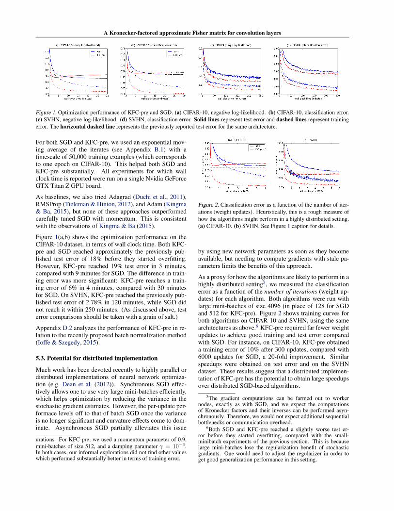
Figure 1. Optimization performance of KFC-pre and SGD. (a) CIFAR-10, negative log-likelihood. (b) CIFAR-10, classification error.(c) SVHN, negative log-likelihood. (d) SVHN, classification error. Solid lines represent test error and dashed lines represent trainingerror. The horizontal dashed line represents the previously reported test error for the same architecture.

For both SGD and KFC-pre, we used an exponential mov-ing average of the iterates (see Appendix B.1) with atimescale of 50,000 training examples (which correspondsto one epoch on CIFAR-10). This helped both SGD andKFC-pre substantially. All experiments for which wallclock time is reported were run on a single Nvidia GeForceGTX Titan Z GPU board.

As baselines, we also tried Adagrad (Duchi et al., 2011),RMSProp (Tieleman & Hinton, 2012), and Adam (Kingma& Ba, 2015), but none of these approaches outperformedcarefully tuned SGD with momentum. This is consistentwith the observations of Kingma & Ba (2015).

Figure 1(a,b) shows the optimization performance on theCIFAR-10 dataset, in terms of wall clock time. Both KFC-pre and SGD reached approximately the previously pub-lished test error of 18% before they started overfitting.However, KFC-pre reached 19% test error in 3 minutes,compared with 9 minutes for SGD. The difference in train-ing error was more significant: KFC-pre reaches a train-ing error of 6% in 4 minutes, compared with 30 minutesfor SGD. On SVHN, KFC-pre reached the previously pub-lished test error of 2.78% in 120 minutes, while SGD didnot reach it within 250 minutes. (As discussed above, testerror comparisons should be taken with a grain of salt.)

Appendix D.2 analyzes the performance of KFC-pre in re-lation to the recently proposed batch normalization method(Ioffe & Szegedy, 2015).

5.3. Potential for distributed implementation

Much work has been devoted recently to highly parallel ordistributed implementations of neural network optimiza-tion (e.g. Dean et al. (2012)). Synchronous SGD effec-tively allows one to use very large mini-batches efficiently,which helps optimization by reducing the variance in thestochastic gradient estimates. However, the per-update per-formace levels off to that of batch SGD once the varianceis no longer significant and curvature effects come to dom-inate. Asynchronous SGD partially alleviates this issue

urations. For KFC-pre, we used a momentum parameter of 0.9,mini-batches of size 512, and a damping parameter � = 10�3.In both cases, our informal explorations did not find other valueswhich performed substantially better in terms of training error.

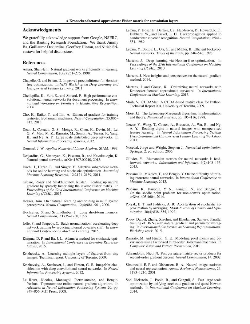
Figure 2. Classification error as a function of the number of iter-ations (weight updates). Heuristically, this is a rough measure ofhow the algorithms might perform in a highly distributed setting.(a) CIFAR-10. (b) SVHN. See Figure 1 caption for details.

by using new network parameters as soon as they becomeavailable, but needing to compute gradients with stale pa-rameters limits the benefits of this approach.

As a proxy for how the algorithms are likely to perform in ahighly distributed setting5, we measured the classificationerror as a function of the number of iterations (weight up-dates) for each algorithm. Both algorithms were run withlarge mini-batches of size 4096 (in place of 128 for SGDand 512 for KFC-pre). Figure 2 shows training curves forboth algorithms on CIFAR-10 and SVHN, using the samearchitectures as above.6 KFC-pre required far fewer weightupdates to achieve good training and test error comparedwith SGD. For instance, on CIFAR-10, KFC-pre obtaineda training error of 10% after 300 updates, compared with6000 updates for SGD, a 20-fold improvement. Similarspeedups were obtained on test error and on the SVHNdataset. These results suggest that a distributed implemen-tation of KFC-pre has the potential to obtain large speedupsover distributed SGD-based algorithms.

5The gradient computations can be farmed out to workernodes, exactly as with SGD, and we expect the computationsof Kronecker factors and their inverses can be performed asyn-chronously. Therefore, we would not expect additional sequentialbottlenecks or communication overhead.

6Both SGD and KFC-pre reached a slightly worse test er-ror before they started overfitting, compared with the small-minibatch experiments of the previous section. This is becauselarge mini-batches lose the regularization benefit of stochasticgradients. One would need to adjust the regularizer in order toget good generalization performance in this setting.


AcknowledgmentsWe gratefully acknowledge support from Google, NSERC,and the Banting Research Foundation. We thank JimmyBa, Guillaume Desjardins, Geoffrey Hinton, and Nitish Sri-vastava for helpful discussions.

ReferencesAmari, Shun-Ichi. Natural gradient works efficiently in learning.

Neural Computation, 10(2):251–276, 1998.

Chapelle, O. and Erhan, D. Improved preconditioner for Hessian-free optimization. In NIPS Workshop on Deep Learning andUnsupervised Feature Learning, 2011.

Chellapilla, K., Puri, S., and Simard, P. High performance con-volutional neural networks for document processing. In Inter-national Workshop on Frontiers in Handwriting Recognition,2006.

Cho, K., Raiko, T., and Ilin, A. Enhanced gradient for trainingrestricted Boltzmann machines. Neural Computation, 25:805–813, 2013.

Dean, J., Corrado, G. S., Monga, R., Chen, K., Devin, M., Le,Q. V., Mao, M. Z., Ranzato, M., Senior, A., Tucker, P., Yang,K., and Ng, A. Y. Large scale distributed deep networks. InNeural Information Processing Systems, 2012.

Demmel, J. W. Applied Numerical Linear Algebra. SIAM, 1997.

Desjardins, G., Simonyan, K., Pascanu, R., and Kavukcuoglu, K.Natural neural networks. arXiv:1507.00210, 2015.

Duchi, J., Hazan, E., and Singer, Y. Adaptive subgradient meth-ods for online learning and stochastic optimization. Journal ofMachine Learning Research, 12:2121–2159, 2011.

Grosse, Roger and Salakhutdinov, Ruslan. Scaling up naturalgradient by sparsely factorizing the inverse Fisher matrix. InProceedings of the 32nd International Conference on MachineLearning (ICML), 2015.

Heskes, Tom. On “natural” learning and pruning in multilayeredperceptrons. Neural Computation, 12(4):881–901, 2000.

Hochreiter, S. and Schmidhuber, J. Long short-term memory.Neural Computation, 9:1735–1780, 1997.

Ioffe, S. and Szegedy, C. Batch normalization: accelerating deepnetwork training by reducing internal covariate shift. In Inter-national Conference on Machine Learning, 2015.

Kingma, D. P. and Ba, J. L. Adam: a method for stochastic opti-mization. In International Conference on Learning Represen-tations, 2015.

Krizhevsky, A. Learning multiple layers of features from tinyimages. Technical report, University of Toronto, 2009.

Krizhevsky, A., Sutskever, I., and Hinton, G. E. ImageNet clas-sification with deep convolutional neural networks. In NeuralInformation Processing Systems, 2012.

Le Roux, Nicolas, Manzagol, Pierre-antoine, and Bengio,Yoshua. Topmoumoute online natural gradient algorithm. InAdvances in Neural Information Processing Systems 20, pp.849–856. MIT Press, 2008.

LeCun, Y., Boser, B., Denker, J. S., Henderson, D., Howard, R. E.,Hubbard, W., and Jackel, L. D. Backpropagation applied tohandwritten zip code recognition. Neural Computation, 1:541–551, 1989.

LeCun, Y., Bottou, L., Orr, G., and Muller, K. Efficient backprop.Neural networks: Tricks of the trade, pp. 546–546, 1998.

Martens, J. Deep learning via Hessian-free optimization. InProceedings of the 27th International Conference on MachineLearning (ICML), 2010.

Martens, J. New insights and perspectives on the natural gradientmethod, 2014.

Martens, J. and Grosse, R. Optimizing neural networks withKronecker-factored approximate curvature. In InternationalConference on Machine Learning, 2015.

Mnih, V. CUDAMat: A CUDA-based matrix class for Python.Technical Report 004, University of Toronto, 2009.

More, J.J. The Levenberg-Marquardt algorithm: implementationand theory. Numerical analysis, pp. 105–116, 1978.

Netzer, Y., Wang, T., Coates, A., Bissacco, A., Wu, B., and Ng,A. Y. Reading digits in natural images with unsupervisedfeature learning. In Neural Information Processing SystemsDeep Learning and Unsupervised Feature Learning Workshop,2011.

Nocedal, Jorge and Wright, Stephen J. Numerical optimization.Springer, 2. ed. edition, 2006.

Ollivier, Y. Riemannian metrics for neural networks I: feed-forward networks. Information and Inference, 4(2):108–153,2015.

Pascanu, R., Mikolov, T., and Bengio, Y. On the difficulty of train-ing recurrent neural networks. In International Conference onMachine Learning, 2013.

Pascanu, R., Dauphin, Y. N., Ganguli, S., and Bengio, Y.On the saddle point problem for non-convex optimization.arXiv:1405.4604, 2014.

Polyak, B. T. and Juditsky, A. B. Acceleration of stochastic ap-proximation by averaging. SIAM Journal of Control and Opti-mization, 30(4):838–855, 1992.

Povey, Daniel, Zhang, Xiaohui, and Khudanpur, Sanjeev. Paralleltraining of DNNs with natural gradient and parameter averag-ing. In International Conference on Learning Representations:Workshop track, 2015.

Ranzato, M. and Hinton, G. E. Modeling pixel means and co-variances using factorized third-order Boltzmann machines. InComputer Vision and Pattern Recognition, 2010.

Schraudolph, Nicol N. Fast curvature matrix-vector products forsecond-order gradient descent. Neural Computation, 14, 2002.

Simoncelli, E. P. and Olshausen, B. A. Natural image statisticsand neural representation. Annual Review of Neuroscience, 24:1193–1216, 2001.

Sohl-Dickstein, J., Poole, B., and Ganguli, S. Fast large-scaleoptimization by unifying stochastic gradient and quasi-Newtonmethods. In International Conference on Machine Learning,2014.


Srivastava, N. Improving neural networks with dropout. Master’sthesis, University of Toronto, 2013.

Srivastava, N. Toronto Deep Learning ConvNet. https:

//github.com/TorontoDeepLearning/convnet/,2015.

Sutskever, I., Vinyals, O., and Le, Q. V. V. Sequence to sequencelearning with neural networks. In Neural Information Process-ing Systems, 2014.

Swersky, K., Chen, Bo, Marlin, B., and de Freitas, N. A tu-torial on stochastic approximation algorithms for training re-stricted Boltzmann machines and deep belief nets. In Informa-tion Theory and Applications Workshop (ITA), 2010, pp. 1–10,Jan 2010.

Tieleman, T. and Hinton, G. Lecture 6.5, RMSProp. In Courseracourse Neural Networks for Machine Learning, 2012.

Vatanen, Tommi, Raiko, Tapani, Valpola, Harri, and LeCun,Yann. Pushing stochastic gradient towards second-order meth-ods – backpropagation learning with transformations in non-linearities. 2013.

Vinyals, O. and Povey, D. Krylov subspace descent for deep learn-ing. In International Conference on Artificial Intelligence andStatistics (AISTATS), 2012.

Yang, Z., Moczulski, M., Denil, M., de Freitas, N., Smola, A.,Song, L., and Wang, Z. Deep fried convnets. arXiv:1412.7149,2014.

Zeiler, Matthew D. ADADELTA: An adaptive learning ratemethod. 2013.

.

https://github.com/TorontoDeepLearning/convnet/

https://github.com/TorontoDeepLearning/convnet/

Documents

A Kronecker-factored approximate Fisher matrix for convolution layers