A Introduction to Matrix Algebra and the Normal · Today’s Class • An introduction to matrix algebra Scalars, vectors, and matrices Basic matrix operations Advanced matrix operations

A Introduction to Matrix Algebraand the Multivariate Normal Distribution

PRE 905: Multivariate AnalysisSpring 2014Lecture 6

PRE 905: Lecture 7 ‐‐Matrix Algebra and the MVN Distribution

Today’s Class

• An introduction to matrix algebra Scalars, vectors, and matrices Basic matrix operations Advanced matrix operations

• An introduction to matrices in R Embedded within the R language

PRE 905: Lecture 7 ‐‐Matrix Algebra and the MVN Distribution 2

Why Learning a Little Matrix Algebra is Important

• Matrix algebra is the alphabet of the language of statistics You will most likely encounter formulae with matrices very quickly

• For example, imagine you were interested in analyzing some repeated measures data…but things don’t go as planned From the SAS User’s Guide (PROC MIXED):


Introduction and Motivation

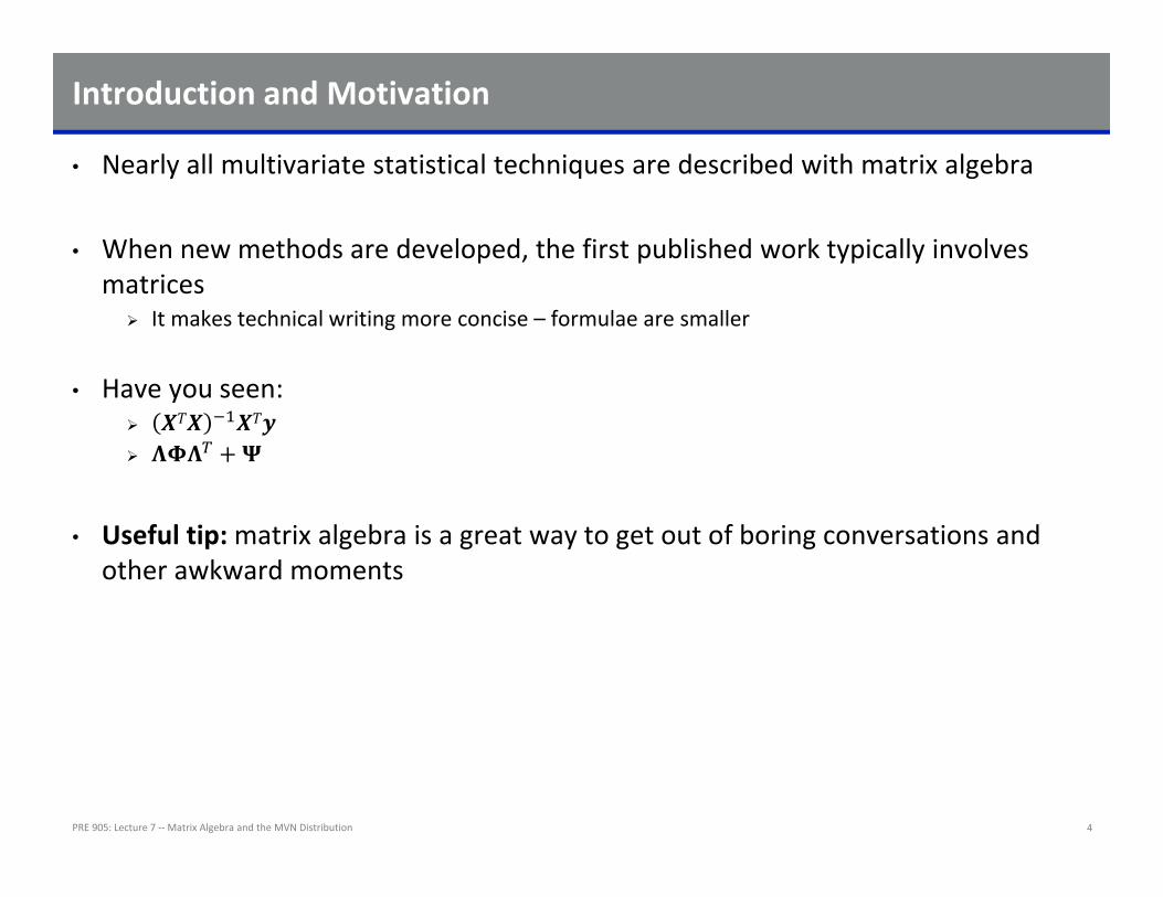
• Nearly all multivariate statistical techniques are described with matrix algebra

• When new methods are developed, the first published work typically involves matrices It makes technical writing more concise – formulae are smaller

• Have you seen:

• Useful tip:matrix algebra is a great way to get out of boring conversations and other awkward moments


Definitions

• We begin this class with some general definitions (from dictionary.com): Matrix:

1. A rectangular array of numeric or algebraic quantities subject to mathematical operations

2. The substrate on or within which a fungus grows

Algebra:1. A branch of mathematics in which symbols, usually letters of the alphabet,

represent numbers or members of a specified set and are used to represent quantities and to express general relationships that hold for all members of the set

2. A set together with a pair of binary operations defined on the set. Usually, the set and the operations include an identity element, and the operations are commutative or associative


Why Learn Matrix Algebra

• Matrix algebra can seem very abstract from the purposes of this class (and statistics in general)

• Learning matrix algebra is important for: Understanding how statistical methods work

And when to use them (or not use them) Understanding what statistical methods mean Reading and writing results from new statistical methods

• Today’s class is the first lecture of learning the language of multivariate statistics


DATA EXAMPLE AND R


A Guiding Example

• To demonstrate matrix algebra, we will make use of data• Imagine that somehow I collected data SAT test scores for both the Math (SATM) and

Verbal (SATV) sections of 1,000 students

• The descriptive statistics of this data set are given below:


The Data…


In Excel: In SAS:

DEFINITIONS OF MATRICES, VECTORS, AND SCALARS


Matrices

• A matrix is a rectangular array of data Used for storing numbers

• Matrices can have unlimited dimensions For our purposes all matrices will have two dimensions:

Row Columns

• Matrices are symbolized by boldface font in text, typically with capital letters Size (r rows x c columns)


SAT Verbal (Column 1)

SAT Math (Column 2)

Vectors

• A vector is a matrix where one dimension is equal to size 1 Column vector: a matrix of size 1

·

520520⋮

540

Row vector: a matrix of size 1 · 520 580

• Vectors are typically written in boldface font text, usually with lowercase letters

• The dots in the subscripts · and · represent the dimension aggregated across in the vector · is the first row and all columns of · is the first column and all rows of Sometimes the rows and columns are separated by a comma (making it possible to read double‐digits in either dimension)


Matrix Elements

• A matrix (or vector) is composed of a set of elements Each element is denoted by its position in the matrix (row and column)

• For our matrix of data (size 1000 rows and 2 columns), each element is denoted by:

The first subscript is the index for the rows: i = 1,…,r (= 1000) The second subscript is the index for the columns: j = 1,…,c (= 2)

⋮ ⋮, ,


Scalars

• A scalar is just a single number

• The name scalar is important: the number “scales” a vector – it can make a vector “longer” or “shorter”

• Scalars are typically written without boldface:520

• Each element of a matrix is a scalar


Matrix Transpose

• The transpose of a matrix is a reorganization of the matrix by switching the indices for the rows and columns

520 580520 550⋮ ⋮

540 660

520 520 ⋯ 540580 550 ⋯ 660

• An element in the original matrix is now in the transposed matrix

• Transposes are used to align matrices for operations where the sizes of matrices matter (such as matrix multiplication)


Types of Matrices

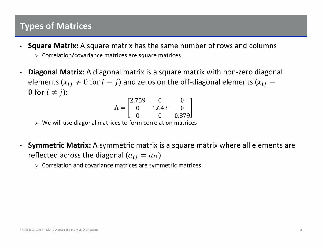
• Square Matrix: A square matrix has the same number of rows and columns Correlation/covariance matrices are square matrices

• Diagonal Matrix: A diagonal matrix is a square matrix with non‐zero diagonal elements ( 0for and zeros on the off‐diagonal elements (0for ):

2.759 0 00 1.643 00 0 0.879

We will use diagonal matrices to form correlation matrices

• Symmetric Matrix: A symmetric matrix is a square matrix where all elements are reflected across the diagonal ( Correlation and covariance matrices are symmetric matrices


VECTORS


Vectors in Space…

• Vectors (row or column) can be represented as lines on a Cartesian coordinate system (a graph)

• Consider the vectors: 12 and 2

3• A graph of these vectors would be:

• Question: how would a column vector for each of our example variables (SATM and SATV) be plotted?


Vector Length

• The length of a vector emanating from the origin is given by the Pythagorean formula This is also called the Euclidean distance between the endpoint of the vector and the origin

⋯

• From the last slide: 5 2.24; 13 3.61

• From our data: 15,868.138; 15,964.42

• In data: length is an analog to the standard deviation In mean‐centered variables, the length is the square root of the sum of mean deviations (not quite the

SD, but close)


Vector Addition

• Vectors can be added together so that a new vector is formed

• Vector addition is done element‐wise, by adding each of the respective elements together: The new vector has the same number of rows and columns

12

23

35

Geometrically, this creates a new vector along either of the previous two Starting at the origin and ending at a new point in space

• In Data: a new variable (say, SAT total) is the result of vector addition. .


Vector Addition: Geometrically


Vector Multiplication by Scalar

• Vectors can be multiplied by scalars All elements are multiplied by the scalar

2 2 12

24

• Scalar multiplication changes the length of the vector:2 4 20 4.47

• This is where the term scalar comes from: a scalar ends up “rescaling” (resizing) a vector

• In Data: the GLM (where X is a matrix of data) the fixed effects (slopes) are scalars multiplying the data


Scalar Multiplication: Geometrically


Linear Combinations

• Addition of a set of vectors (all multiplied by scalars) is called a linear combination:⋯

• Here, is the linear combination For all k vectors, the set of all possible linear combinations is called their span Typically not thought of in most analyses – but when working with things that don’t exist (latent

variables) becomes somewhat important

• In Data: linear combinations happen frequently: Linear models (i.e., Regression and ANOVA) Principal components analysis


Linear Dependencies

• A set of vectors are said to be linearly dependent if⋯ 0

‐and‐, , … , are all not zero

• Example: let’s make a new variable – SAT Total:1 ∗ 1 ∗

• The new variable is linearly dependent with the others:1 ∗ 1 ∗ 1 ∗

• In Data: (multi) collinearity is a linear dependency. Linear dependencies are bad for statistical analyses that use matrix inverses


Inner (Dot) Product of Vectors

• An important concept in vector geometry is that of the inner product of two vectors The inner product is also called the dot product

· ⋯

• The dot or inner product is related to the angle between vectors and to the projection of one vector onto another

• From our example: · 1 ∗ 2 2 ∗ 3 8• From our data: . ⋅ . 251,928,400

• In data: the angle between vectors is related to the correlation between variables and the projection is related to regression/ANOVA/linear models


Angle Between Vectors

• As vectors are conceptualized geometrically, the angle between two vectors can be calculated

cos·

• From the example:

cos85 13

0.12

• From our data:

, cos251,928,400

15,868.138 15,946.420.105


In Data: Cosine Angle = Correlation

• If you have data that are: Placed into vectors Centered by the mean (subtract the mean from each observation)

• …then the cosine of the angle between those vectors is the correlation between the variables:

· ∑

∑ ∑

For the SAT example data (using mean centered variables):

, cos , cos3,132,223.6

1,573.956 ∗ 2,567.0425 .775


Vector Projections

• A final vector property that shows up in statistical terms frequently is that of a projection

• The projection of a vector onto is the orthogonal projection of onto the straight line defined by The projection is the “shadow” of one vector onto the other:

·

• In data: linear models can bethought of as projections


Vector Projections Example

• To provide a bit more context for vector projections, let’s consider the projection of mean centered SATV onto SATM:

·

• The first portion turns out to be:· 3,132,223.6

1,573.956 .475

• This is also the regression slope :


MATRIX ALGEBRA


Moving from Vectors to Matrices

• A matrix can be thought of as a collection of vectors Matrix operations are vector operations on steroids

• Matrix algebra defines a set of operations and entities on matrices I will present a version meant to mirror your previous algebra experiences

• Definitions: Identity matrix Zero vector Ones vector

• Basic Operations: Addition Subtraction Multiplication “Division”


Matrix Addition and Subtraction

• Matrix addition and subtraction are much like vector addition/subtraction

• Rules: Matrices must be the same size (rows and columns)

• Method: The new matrix is constructed of element‐by‐element addition/subtraction of the previous matrices

• Order: The order of the matrices (pre‐ and post‐) does not matter


Matrix Addition/Subtraction


Matrix Multiplication

• Matrix multiplication is a bit more complicated The new matrix may be a different size from either of the two

multiplying matrices

• Rules: Pre‐multiplying matrix must have number of columns equal to the number of rows of the post‐

multiplying matrix

• Method: The elements of the new matrix consist of the inner (dot) product of the row vectors of the pre‐

multiplying matrix and the column vectors of the post‐multiplying matrix

• Order: The order of the matrices (pre‐ and post‐) matters


Matrix Multiplication


Multiplication in Statistics

• Many statistical formulae with summation can be re‐expressed with matrices

• A common matrix multiplication form is: Diagonal elements: ∑ Off‐diagonal elements: ∑

• For our SAT example:

251,797,800 251,928,400251,928,400 254,862,700


Identity Matrix

• The identity matrix is a matrix that, when pre‐ or post‐multiplied by another matrix results in the original matrix:

• The identity matrix is a square matrix that has: Diagonal elements = 1 Off‐diagonal elements = 0

1 0 00 1 00 0 1


Zero Vector

• The zero vector is a column vector of zeros

000

• When pre‐ or post‐multiplied the result is the zero vector:


Ones Vector

• A ones vector is a column vector of 1s:

111

• The ones vector is useful for calculating statistical terms, such as the mean vector and the covariance matrix


Matrix “Division”: The Inverse Matrix

• Division from algebra: First:

Second: 1

• “Division” in matrices serves a similar role For square and symmetric matrices, an inverse matrix is a matrix that when pre‐ or post‐multiplied with

another matrix produces the identity matrix:

• Calculation of the matrix inverse is complicated Even computers have a tough time

• Not all matrices can be inverted Non‐invertible matrices are called singular matrices

In statistics, singular matrices are commonly caused by linear dependencies


The Inverse

• In data: the inverse shows up constantly in statistics Models which assume some type of (multivariate) normality need an inverse covariance matrix

• Using our SAT example Our data matrix was size (1000 x 2), which is not invertible However was size (2 x 2) – square, and symmetric

251,797,800 251,928,400251,928,400 254,862,700

The inverse is:3.61 7 3.57 73.57 7 3.56 7


Matrix Algebra Operations

•

•

•

•

•

•

•

•

•

•

•

• For such that exists:


ADVANCED MATRIX OPERATIONS


Advanced Matrix Functions/Operations

• We end our matrix discussion with some advanced topics All related to multivariate statistical analysis

• To help us throughout, let’s consider the correlation matrix of our SAT data:

1.00 0.780.78 1.00


Matrix Trace

• For a square matrix with p rows/columns, the trace is the sum of the diagonal elements:

• For our data, the trace of the correlation matrix is 2 For all correlation matrices, the trace is equal to the number of variables because all diagonal elements

are 1

• The trace is considered the total variance in multivariate statistics Used as a target to recover when applying statistical models


Matrix Determinants

• A square matrix can be characterized by a scalar value called a determinant:det

• Calculation of the determinant is tedious Our determinant was 0.3916

• The determinant is useful in statistics: Shows up in multivariate statistical distributions Is a measure of “generalized” variance of multiple variables

• If the determinant is positive, the matrix is called positive definite Is invertible

• If the determinant is not positive, the matrix is called non‐positive definite Not invertible


MULTIVARIATE STATISTICS AND DISTRIBUTIONS


Multivariate Statistics

• Up to this point in this course, we have focused on the prediction (or modeling) of a single variable Conditional distributions (aka, generalized linear models)

• Multivariate statistics is about exploring joint distributions How variables relate to each other simultaneously

• Therefore, we must adapt our conditional distributions to have multiple variables, simultaneously (later, as multiple outcomes)

• We will now look at the joint distributions of two variables , or in matrix form: (where is size N x 2; gives a scalar/single number) Beginning with two, then moving to anything more than two We will begin by looking at multivariate descriptive statistics

Mean vectors and covariance matrices

• Today, we will only consider the joint distribution of sets of variables – but next time we will put this into a GLM‐like setup The joint distribution will the be conditional on other variables


Multiple Means: The Mean Vector

• We can use a vector to describe the set of means for our data

1⋮

Here is a N x 1 vector of 1s The resulting mean vector is a v x 1 vector of means

• For our data:499.32499.27

• In R:


Mean Vector: Graphically

• The mean vector is the center of the distribution of both variables


200

400

600

800

200 400 600 800

SATV

SATM

Covariance of a Pair of Variables

• The covariance is a measure of the relatedness Expressed in the product of the units of the two variables:

1

The covariance between SATV and SATM was 3,132.22 (in SAT Verbal‐Maths) The denominator N is the ML version – unbiased is N‐1

• Because the units of the covariance are difficult to understand, we more commonly describe association (correlation) between two variables with correlation Covariance divided by the product of each variable’s standard deviation


Correlation of a Pair of Varibles

• Correlation is covariance divided by the product of the standard deviation of each variable:

The correlation between SATM and SATV was 0.78

• Correlation is unitless – it only ranges between ‐1 and 1 If and both had variances of 1, the covariance between them would be a correlation

Covariance of standardized variables = correlation


Covariance and Correlation in Matrices

• The covariance matrix (for any number of variables v) is found by:

1 ⋯⋮ ⋱ ⋮

⋯

•2,477.34 3,123.223,132.22 6,589.71

• In R:


From Covariance to Correlation

• If we take the SDs (the square root of the diagonal of the covariance matrix) and put them into a diagonal matrix , the correlation matrix is found by:

⋯

⋮ ⋱ ⋮

⋯

1 ⋯⋮ ⋱ ⋮

⋯ 1


Example Covariance Matrix

• For our data, the covariance matrix was:2,477.34 3,123.223,132.22 6,589.71

• The diagonal matrix was:2,477.34 00 6,589.71

49.77 00 81.18

• The correlation matrix was:1

49.77 0

01

81.18

2,477.34 3,123.223,132.22 6,589.71

149.77 0

01

81.18 1.00 .78

.78 1.00


In R:


Generalized Variance

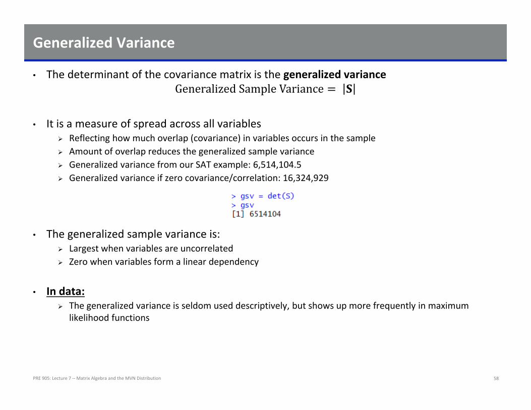
• The determinant of the covariance matrix is the generalized varianceGeneralizedSampleVariance

• It is a measure of spread across all variables Reflecting how much overlap (covariance) in variables occurs in the sample Amount of overlap reduces the generalized sample variance Generalized variance from our SAT example: 6,514,104.5 Generalized variance if zero covariance/correlation: 16,324,929

• The generalized sample variance is: Largest when variables are uncorrelated Zero when variables form a linear dependency

• In data: The generalized variance is seldom used descriptively, but shows up more frequently in maximum

likelihood functions


Total Sample Variance

• The total sample variance is the sum of the variances of each variable in the sample The sum of the diagonal elements of the sample covariance matrix The trace of the sample covariance matrix

tr

• Total sample variance for our SAT example:

• The total sample variance does not take into consideration the covariances among the variables Will not equal zero if linearly dependency exists

• In data: The total sample variance is commonly used as the denominator (target) when calculating variance

accounted for measures


MULTIVARIATE DISTRIBUTIONS (VARIABLES ≥ 2)


Multivariate Normal Distribution

• The multivariate normal distribution is the generalization of the univariate normal distribution to multiple variables The bivariate normal distribution just shown is part of the MVN

• The MVN provides the relative likelihood of observing all V variables for a subject p simultaneously:

…

• The multivariate normal density function is:

1

2exp 2


The Multivariate Normal Distribution

1

2exp 2

• The mean vector is ⋮

• The covariance matrix is

⋯⋯

⋮ ⋮ ⋱ ⋮⋯

The covariance matrix must be non‐singular (invertible)


Comparing Univariate and Multivariate Normal Distributions

• The univariate normal distribution:12

exp 2

• The univariate normal, rewritten with a little algebra:

1

2 | |exp 2

• The multivariate normal distribution

1

2exp 2

When 1 (one variable), the MVN is a univariate normal distribution


The Exponent Term

• The term in the exponent (without the ) is called the squared Mahalanobis Distance

Sometimes called the statistical distance

Describes how far an observation is from its mean vector, in standardized units

Like a multivariate Z score (but, if data are MVN, is actually distributed as a variable with DF = number of variables in X)

Can be used to assess if data follow MVN


Multivariate Normal Notation

• Standard notation for the multivariate normal distribution of v variables is , Our SAT example would use a bivariate normal: ,

• In data: The multivariate normal distribution serves as the basis for most every statistical technique commonly

used in the social and educational sciences General linear models (ANOVA, regression, MANOVA) General linear mixed models (HLM/multilevel models) Factor and structural equation models (EFA, CFA, SEM, path models) Multiple imputation for missing data

Simply put, the world of commonly used statistics revolves around the multivariate normal distribution Understanding it is the key to understanding many statistical methods


Bivariate Normal Plot #1

00 , 1 0

0 1


Density Surface (3D) Density Surface (2D): Contour Plot

Bivariate Normal Plot #2 (Multivariate Normal)

00 , 1 .5

.5 1


Density Surface (3D) Density Surface (2D): Contour Plot

Multivariate Normal Properties

• The multivariate normal distribution has some useful properties that show up in statistical methods

• If is distributed multivariate normally:1. Linear combinations of are normally distributed

2. All subsets of are multivariate normally distributed

3. A zero covariance between a pair of variables of implies that the variables are independent

4. Conditional distributions of are multivariate normal


Multivariate Normal Distribution in PROC IML

• To demonstrate how the MVN works, we will now investigate how the PDF provides the likelihood (height) for a given observation: Here we will use the SAT data and assume the sample mean vector and covariance matrix are known to

be the true:499.32498.27 ; 2,477.34 3,123.22

3,132.22 6,589.71

• We will compute the likelihood value for several observations (SEE EXAMPLE R SYNTAX FOR HOW THIS WORKS): ,⋅ 590 730 ; 0.0000001393048 ,⋅ 340 300 ; 0.0000005901861 499.32 498.27 ; 0.000009924598

• Note: this is the height for these observations, not the joint likelihood across all the data Next time we will use PROC MIXED to find the parameters in and using maximum likelihood


Likelihoods…From R


1

2 exp 2

WRAPPING UP


Wrapping Up

• Matrix algebra is the language of multivariate statistics Learning the basics will help you read work (both new old)

• Over the course of the rest of the semester, we will use matrix algebra frequently It provides for more concise formulae

• In practice, we will use matrix algebra very little But understanding how it works is the key to understanding how statistical methods work and are

related


Wrapping Up

• The last two classes set the stage to discuss multivariate statistical methods that use maximum likelihood

• Matrix algebra was necessary so as to concisely talk about our distributions (which will soon be models)

• The multivariate normal distribution will be necessary to understand as it is the most commonly used distribution for estimation of multivariate models

• Next week we will get back into data analysis – but for multivariate observations…using R’s LME4 package (and the lmer() function) Each term of the MVN will be mapped onto the lmer() output


Documents

A Introduction to Matrix Algebra and the Normal · Today’s Class • An introduction to matrix algebra Scalars, vectors, and matrices Basic matrix operations Advanced matrix operations