Embed Size (px)
Citation preview

IIE Transactions on Healthcare Systems Engineering (2015) 5, 14–32Copyright C© “IIE”ISSN: 1948-8300 print / 1948-8319 onlineDOI: 10.1080/19488300.2014.993006
A hybrid prediction model for no-shows and cancellationsof outpatient appointments
ADEL ALAEDDINI1,∗, KAI YANG2, PAMELA REEVES3 and CHANDAN K. REDDY4
1Department of Mechanical Engineering, University of Texas at San Antonio, San Antonio, TX, USAE-mail: [email protected] of Industrial and Systems Engineering, Wayne State University, Detroit, MI, USA3Dingell VA Medical Center, MI, USA4Department of Computer Science, Wayne State University, Detroit, MI, USA
Received June 2012 and accepted October 2014
A no-show occurs when a scheduled patient neither keeps nor cancels the appointment. A cancellation happens when individualscontact the clinic and cancel their scheduled appointments. Such disruptions not only cause inconvenience to hospital management,they also have a significant impact on the revenue, cost and resource utilization for almost all of the healthcare systems. In thispaper, we develop a hybrid probabilistic model based on multinomial logistic regression and Bayesian inference to predict accuratelythe probability of no-show and cancellation in real-time. First, a multinomial logistic regression model is built based on the entirepopulation’s general social and demographic information to provide initial estimates of no-show and cancellation probabilities. Next,the estimated probabilities from the logistic model are transformed into a bivariate Dirichlet distribution, which is used as the priordistribution of a Bayesian updating mechanism to personalize the initial estimates for each patient based on his/her attendancerecord. In addition, to further improve the estimates, prior to applying the Bayesian updating mechanism, each appointment in thedatabase is weighted based on its recency, weekday of occurrence, and clinic type. The effectiveness of the proposed approach isdemonstrated using healthcare data collected at a medical center. We also discuss the advantages of the proposed hybrid model anddescribe possible real-world applications.
Keywords: Multinomial logistic regression, Dirichlet distribution, Bayesian inference, healthcare operations improvement, no-showand cancellation prediction
1. Introduction
The problem of appointment no-show and cancellation,which is also known as appointment disruption, can causesignificant disturbance in the smooth operation of almostall scheduling systems. When scheduled patients do not at-tend their appointments, resources will be underutilized,while other patients cannot get timely appointments be-cause part of the schedule is filled with patients who will notattend. Also, when scheduled patients cancel their appoint-ments, they often leave the clinic with a very short amountof time to fill the schedule. In such cases, overbooking canhelp to some extent, but it usually results in clinic conges-tion and patient dissatisfaction. In fact, appointment no-show and cancellation have far-reaching effects on clinicefficiency, patient outcomes, and healthcare costs, whichcan reach hundreds of thousands of dollars yearly (Moore
∗Corresponding authorColor versions of one or more of the figures in the article can
be found online at www.tandfonline.com/uhse.
et al., 2001; Bech, 2005; Hixon et al., 1999; Rust et al,. 1995;Barron, 1980). Hence, accurate prediction of no-show andcancellation probability is a cornerstone for any schedul-ing system and non-attendance reduction strategy (Daggyet al., 2010; Cayirli and Veral, 2003; Ho and Lau, 1992;Cote, 1999; Hixon et al., 1999; and Moore et al., 2001).
In this article, we develop a hybrid probabilistic modelbased on multinomial logistic regression and Bayesian in-ference to predict accurately the probability of no-showsand cancellations in real-time. The result of the proposedmethod can be used to develop more effective appoint-ment scheduling (Chakraborty et al., 2010; Glowacka et al.,2009; Gupta and Denton, 2008; Hassin and Mendel, 2008;Liu et al., 2009). It can also be used for developing effec-tive strategies, such as selective overbooking for reducingthe negative effects of disturbances and filling appointmentslots while maintaining short waiting times (Laganga andLawrence, 2007; Muthuraman and Lawley, 2008; and Zenget al., 2010).
The rest of the article is organized as follows: Sec-tion 2 summarizes some of the related work proposed
1948-8300 C© 2015 “IIE”
Dow
nloa
ded
by [
Cha
ndan
Red
dy]
at 1
1:44
18
Mar
ch 2
015
A hybrid prediction model 15
in the literature. Section 3 describes the general schemeof the proposed model. Section 4 explains our proposedalgorithm for predicting no-show and cancellation prob-abilities. Section 5 presents the results of applying theproposed prediction model to a healthcare dataset col-lected at a medical center. Finally, Section 6 concludes ourwork and presents some future extensions of the proposedmodel.
2. Relevant background and problem formulation
Turkcan et al. ([2013)] provide a structured and represen-tative review of no-show literature (see also Rowett et al.,2010; Bowser et al,. 2010; Denhaerynck et al., 200; andGeorge et al., 2003). The rate of no-show in the reviewedarticles varies significantly for different clinical populationof patients, e.g., chronic care, primary care, etc., and lo-cations, e.g., North America, Europe, etc., ranging fromclose to zero up to 48-64% (see also Mitchell and Selmes,(2007),;Bech, 2005; Cayirli et al., 2006, 2008; and Yehiaet al., 2008. Several reasons are reported for no-show in-cluding: forgot appointment, conflict with appointment,transportation, physically/mentally unwellness, schedulingsystem problems, perceived disrespect, bad weather and fi-nancial problems (See also Park et al., 2008; Neal et al.,2005; Tuller et al., 2010; Sarnquist et al., 2011; Corfieldet al., 2008; Gany et al., 2001). Several factors are stud-ied for predicting non-attendance behavior (Daggy et al.,2010; Zeng et al., 2010; Turkcan et al., 2013; Cashman et al.,2004; Cohen et al., 2008; Savageau et al., 2004; Alafaireet,2010; Lehmann, 2007). The literature also shows the rela-tionship between no-show and specific health outcomes insome clinical populations including diabetic, dialysis, hu-man immunodeficiency virus (HIV), primary care and psy-chiatric (Schectman et al., 2008; Obialo et al., 2008; Murphyet al., 2011; Bigby et al., 1984). Ample literature is avail-able discussing interventions to reduce no-show including:appointment reminders, patient education, and follow-upafter a no-show appointment, open-access scheduling, andlean process improvement methods (see also Hardy et al.,2001; Guse et al., 2003; Can et al., 2003; Kopach et al., 2007;Murray and Tantau, 2000; LaGanga, 2011; Fischman,2010; Garuda et al., 1998). In fact, the effectiveness of manyof the above intervention strategies and consequently clin-ics’ performance significantly rely on the accurate predic-tion of individual patients’ risk of non-attendance (Daggyet al., 2010). Below we have divided the related quantita-tive methods of predicting appointment disruption into twogroups of population-based models and individual-basedmodels.
Population-based techniques mainly use a variety of meth-ods drawn from statistics and machine learning that canbe used for predicting no-shows and cancellations (Doveand Schneider, 1981; Kotsiantis, 2007). These methods
use the information from the entire population (dataset)in the form of set factors, in order to estimate the(probability of) no-show, cancellation and attendance(Baldi et al., 2000; Kotsiantis, 2007). Logistic regressionis one of the most popular statistical methods in thiscategory that is used for binomial regression, which canpredict the probability of disturbances by fitting numer-ical or categorical predictor variables in data to a logitfunction (Turkcan et al., 2013; Daggy et al., 2010; Hilbe,2009). There has been some work using tree-based andrule-based models that create if–then constructs to sepa-rate the data into increasingly homogeneous subsets, basedon which of the desired predictions of disturbances canbe made (Glowacka et al., 2009). The problem with thesepopulation- based methods is that although they providea reasonable estimate, they do not differentiate betweenthe behaviors of individuals and hence cannot update ef-fectively, especially using small datasets. Another problemwith these methods is that once the model has been built,adding new data has an insignificant effect on the resultespecially when the size of the initial dataset is much largerthan the size of the new data. In Section 5, we will com-pare the performance of above methods with the proposedapproach.
Individual based approaches are primarily based on time se-ries and smoothing methods, which are used for predictingthe probability of a disruption in an appointment. Thesemethods utilize past behaviors of individuals for the es-timation of future no-show and cancellations probability.Potential time series methods for predicting no-shows andcancellations include autoregressive models (Brockwell,2009), time-frequency analysis models (Chatfield, 1996;and Bloomfield, 1976), nonlinear filtering and HiddenMarkov Models (HMM), Stratonovich (1960). Commonsmoothing algorithms that can be used for no-show andcancellation include moving average, exponential smooth-ing, and local regression (Simonoff, 1996; Cleveland, 1993;and Winter, 1960). While individual-based methods are fastand effective in modeling the behavioral (no-show) patternof each individual and work well with a small dataset, theydo not provide a reliable initial estimate of no-show andcancellation probabilities, which is especially important inour case. The main reason is that individual based meth-ods usually employ a function of past data (attendancerecord) to estimate the probability of a future event, e.g.no-show and cancellation. But for the initial state wherethere is no past history available, such function is inappli-cable, and consequently, individual-based methods usuallyuse random guess for the initial estimate, e.g., probabilityof no-show and cancellation. In Section 5, we will comparethe performance of the above- mentioned methods with theproposed method.
As described above, each of the population-based andindividual-based approaches have some advantages anddisadvantages. However, none of the existing studies for
Dow
nloa
ded
by [
Cha
ndan
Red
dy]
at 1
1:44
18
Mar
ch 2
015
16 Alaeddini et al.
prediction of appointment disruptions have considered us-ing these methods together to overcome their problems andimprove their performance, even though related ideas havebeen successfully employed for fields like universal back-ground model (Reynolds et al., 2000), and recommendersystems (Adomavicius and Tuzhilin, 2005). In the next sec-tion, we develop a hybrid approach that combines logis-tic regression as a population-based approach along withBayesian inference as individual-based approach for pre-diction of disturbances in appointment scheduling. Theproposed approach also contains an efficient linear pro-gramming component to optimize its performance.
Indeed, the proposed approach generalizes and extendsAlaeddini et al. (2010) probabilistic model for no-show es-timation to general types of disruptions, e.g. no-show andcancellation. More specifically, this study extends Alaed-dini et al. (2010) binomial logistic regression model forinitial estimation of no-show to a multinomial logistic re-gression, which can take into account multiple types ofdisruptions, namely no-show and cancellation. It also gen-eralizes Alaeddini et al. (2010) Bayesian updating mecha-nism for personalization of the no-show estimates for eachpatient to general types of disruptions using the Dirichletdistribution instead of the Beta distribution. In addition,while Alaeddini et al. (2010) used a set of discrete sub-weights to weight the appointments based on their recency,this paper employs a modified versions of the generalizedlogistic function (Richards, 1959) to design a continuousweighting system. Above generalizations and extensions,enable the proposed approach to develop one general in-tegrated model (instead of multiple standalone models)based on the same set of variables for considering dif-ferent types of disruptions in appointment scheduling, asthey both can have significant but different impacts on thesystem workload and patients’ waiting time; generally therange of possible solutions to a cancellation case is morediverse than a no-show case. The authors recognize thatthe proposed model implicitly assumes that no-show andcancellation can be predicted by the same set of variables,and while this assumption has been verified for this study,no-show and cancellation may not always have the samepredictors.
Some of the major contributions of this research include:(i) Combining the strengths of multinomial logistic regres-sion to provide a reliable initial estimate of no-show andcancellation, and Bayesian updating to personalize the pre-dictions for each patient based on her/his past attendancebehavior; (ii) Statistical integration of multinomial logis-tic regression and Bayesian inference by transforming theoutput of multinomial logistic regression, which is a multi-nomial distribution, to its conjugate Dirichlet distributionand applying the Bayesian updating to the Dirichlet dis-tribution, which is a continuous distribution with severalgood characteristics, such as flexibility and simplicity ofupdating procedure; (iii) Developing and optimizing a set
of appointment weighting factors including: appointmenttype, recency and weekday of occurrence to further improvethe predictions of the proposed model.
Notably, there is a significant difference betweenthe proposed method and Bayesian logistic regression(O’Brien, and Dunson, 2004). Theoretically, in Bayesianlogistic regression, the main focus is modeling uncertaintiesin the parameters of the model, namely the parameter of amultinomial logistic regression. However, in the proposedmethod, the primary concern is modeling the uncertaintyin the outputs of the model, namely no-show, cancellation,and attendance. In addition, unlike the proposed model,in Bayesian logistic regression, modeling a large number ofvariables can be very challenging; as the number of variablesincrease, efficient computation of posterior parameters getsvery difficult. Finally, while in the proposed method the ap-propriate type of prior is chosen based on the relationshipbetween logistic regression and the Dirichlet distribution,in Bayesian logistic regression, specifying an appropriatechoice of prior is usually trivial.
In Section 5, we compare the performance of the pro-posed hybrid model with the representative algorithmsfrom each of population-based and individual-based ap-proaches.
3. General scheme of the proposed model
The proposed model for predicting patient no-show andcancellation is composed of three major components shownin Figure 1. First, the data set will be preprocessed, and aftercoding discrete variables, a multinomial logistic regressionmodel will be built based on the entire populations’ generalsocial and demographic information to provide an initialestimate of no-show and cancellation probabilities. Second,each appointment in the database will be weighted based onits recency, weekday of occurrence, and clinic type. Third,the personalized probability of no-show and cancellationwill be derived for each individual patient using a compre-hensive Bayesian updating mechanism based on the popu-lation estimate from Step 1 and weighted records of eachindividual in Step 2.
In the rest of this section, we will provide a brief descrip-tion about each of the above components, in the followingorder: (i) Population-based estimate of appointment dis-ruptions: multinomial logistic regression, (ii) Adaptation:personalization of the predictions, and (iii) Appointmentweighting: effect of appointment recency, occurrence onnon-working days and clinic type; where we will present theappointment- weighting component after the adaptationcomponent to better demonstrate its impact (in practice,the appointment-weighting component will be applied be-fore the adaptation component). In Section 4, we will showhow these components are connected together through theproposed integrated algorithm.
Dow
nloa
ded
by [
Cha
ndan
Red
dy]
at 1
1:44
18
Mar
ch 2
015

A hybrid prediction model 17
Fig. 1. The general scheme of the proposed method.
3.1. Population based estimate of appointment disruptions:Multinomial logistic regression
The first component of the proposed method is a multi-nomial logistic regression, which is used for initial (prior)estimation of no-show and cancellation probabilities usingthe (training) dataset of the individuals’ general social anddemographical information. Let X be the set of factors (ex-planatory variables) affecting probability of attendance ofan individual, and let Y be the attendance type includingno-show, cancellation, and attendance. In the preprocess-ing step of this study, the following factors were identified assignificant: (i) Sex, which is considered as a discrete factorwith two possibilities of male and female; (ii) Age, whichis considered as a continuous factor ranging from 25 to92; (iii) Marital Status, which is considered as a discretefactor with four categories of never-married, married, di-vorced and widowed; (iv) Medical Service Coverage, whichis considered as a discrete factor with six categories rangingfrom not service connected, to 50-100% service connected(detail information of each category is available at Depart-ment of Veteran Affairs website); (v) Distance to MedicalCenter (mile), which is considered as a continuous fac-tor and calculated using a free Excel add-on based on thedistance between patients’ residence ZIP and the medicalcenter; and (vi) Clinic Type (cluster), which is consideredas a discrete factor with three categories that are definedby clustering the 271 clinics in the database based on theirdisruption rates (see the Appendix for details). Likelihoodratio chi-square tests for categorical variable and t-tests forcontinuous variables have been used to check the signifi-cance of the factors.
The multinomial logistic regression model F (X, Bk)thentakes the form:
⎧⎪⎪⎪⎪⎨⎪⎪⎪⎪⎩
Pk = exp (XBk)
1+�Kk=0exp (XBk)
, k = 1, 2, . . . , K − 1
and Pk = 1−�k−1i=0 Pi
P0 = exp (XBk)
1+�Kk=0exp (XBk)
(1)
where Pk is the probability of kth event (In this study, we usek = 0, 1, 2, representing no-show, cancellation, and atten-dance, respectively). The unknown vector of parametersBk (Bk = [βk0, βk1, . . . , βkl ]) can be estimated using itera-tive procedures, such as Newton-Raphson method or it-eratively reweighted least squares (IRLS) (Agresti, 2002).Notably, our preliminary analysis of data also shows neg-ative correlation between the appointments occurred onnon-working days and the rates of no-show and cancella-tion (P = 0.116 and 0.218). However, due to its sparsity,addition of such factor makes the data matrix of the regres-sion model severely rank deficient such that the estimationof the model parameter becomes impossible. We addressthis problem by including this factor to the model in a laterstage through another component (appointment weight-ing), which will be discussed in detail later.
Also, the model proposed in the paper implicitly assumesthat no-show and cancellation can be predicted by the sameset of variables. In fact, one of the objectives of this researchwas to develop a unified model (instead of multiple stan-dalone models) to consider different types of disruptionsin appointment scheduling, as they can all have significantimpact on the system workload and patients’ waiting time.However, while our initial statistical analysis has verifiedabove assumption for our dataset, no-show and cancella-tion may not always have same predictors.
Finally, the proposed multinomial logistic regression ap-proach provides a more compact and convenient modelfor estimation no-show and cancellation, in comparisonto using two separated logistic regression models for no-show/show and cancellation/show.
3.1.1. Example 1For better understanding of how the above model appliesto the problem domain, we show a simple case study basedon the dataset used in Section 5 experimental results.
The dataset used for this example (the training dataset)is created by dividing the original dataset of this study intotwo disjoint datasets of approximately equal size, namelytraining and testing. The original datasets contains the
Dow
nloa
ded
by [
Cha
ndan
Red
dy]
at 1
1:44
18
Mar
ch 2
015

18 Alaeddini et al.
Table 1. Descriptive statistics of the training dataset used for fitting multinomial logistic regression
Frequency Rate
No-show Cancellation Show-up No-show Cancellation Show-up
SexFemale 30 33 89 19.74% 21.71% 58.55%Male 214 95 617 23.11% 10.26% 66.63%
Marriage StatusNever Married 63 30 223 19.94% 9.49% 70.57%Married 80 46 181 26.06% 14.98% 58.96%Divorced 64 31 121 29.63% 14.35% 56.02%Widowed 38 19 182 15.90% 7.95% 76.15%
Medical Service Coverage (Predefined Categories)Service Connected <5 56 16 171 23.05% 6.58% 70.37%Service Connected, 50% To 100% 70 53 169 23.97% 18.15% 57.88%Service Connected Less Than 50% 14 4 14 43.75% 12.50% 43.75%Non-Service Connected 75 51 319 16.85% 11.46% 71.69%Non-Service Connected, VA Pension 16 5 29 32.00% 10.00% 58.00%Service Connected <6 6 3 7 37.50% 18.75% 43.75%
Clinic Cluster1 10 28 45 12.05% 33.73% 54.22%2 197 75 618 22.13% 8.43% 69.44%3 38 23 44 36.19% 21.90% 41.90%
Age (Average) 56.53 52.17 60.12Distance To Medical Center (Average) 13.72 15.32 14.87
information of 1543 attendance records of 99 patients;therefore, 1078 attendance records (from 10/1/2009 to12/23/2009) are considered for fitting multinomial logis-tic regression. Table 1 provides some descriptive statisticsabout the training dataset.
Applying model (1) to the above dataset and using it-eratively reweighted least squares (IRLS) method, the pa-rameters of the fitted multinomial logistic regression modelalong with their standard error are computed as shown inTable 2 (because we are modeling a categorical variablewith three mutually exclusive levels, namely no-show, can-cellation and attendance, and because the occurrence ofany one of them automatically implies the non-occurrenceof the remaining two events (P2 = 1− (P0 + P1)), only twosets of regression parameters are estimated (see Model 3)).Meanwhile, the assumption of linear association betweenthe continuous covariates of the model and log odds of no-show and cancellations has been verified to be appropriate.
Now for a sample patient in the dataset with the informa-tion shown in Table 3, based on the estimated coefficients(in Table 2), the probability of no-show, cancellation andattendance is estimated as (0.14, 0.09, 0.77).
3.2. Adaptation: Personalization of the predictions
The result of above multinomial logistic regression is amultinomial distribution with three variables, namely prob-abilities of no-show, cancellation and attendance, wherethe parameters (Pk, k = 0, 1, 2) of such distribution is
estimated based on all patients’ information in the (train-ing) dataset using multinomial logistic regression. Such (ini-tial) estimates can be personalized for each patient basedin her/his individual attendance records (in the trainingdataset) to improve the prediction ability of the model.Bayesian inference is another component of the proposedmethod, which is used for updating the prior estimate ofno-show and cancellation probabilities from multinomiallogistic regression using the dataset of individual patientattendance record (training dataset).
To use Bayes’ theorem, we need a prior distributiong(α pri
)that gives our belief about the possible values of the
parameter vector α = (α1, . . . , αK ) representing the prob-abilities of no-show, cancellation and attendance beforeincorporating the data (Z). The posterior distribution isproportional to prior distribution times likelihood:
g (α pos |Z) = g(α pri
)× f(Z|α pri
)∫1
0 g (a)× f (Z|a) da(2)
In Bayesian statistics, the Dirichlet distribution is a com-mon choice for updating the prior estimate of multino-mial distribution parameters (distribution of the depen-dentvariable in the multinomial logistic regression) because(Bolstad, 2007):
1. The Dirichlet distribution is the conjugate prior of multi-nomial distribution, giving the same posterior distribu-tion as the prior (Dirichlet).
Dow
nloa
ded
by [
Cha
ndan
Red
dy]
at 1
1:44
18
Mar
ch 2
015

Tab
le2.
Fit
ted
mul
tino
mia
llog
isti
cre
gres
sion
mod
el,i
nclu
ding
regr
essi
onco
effic
ient
s,st
anda
rder
ror
and
p-va
lues
Mar
riag
est
atus
Med
ical
serv
ice
cove
rage
Clin
iccl
uste
rD
ista
nce
tom
edic
alSe
xA
geT
ype
1T
ype
2T
ype
3C
at.1
Cat
.2C
at.3
Cat
.4C
at.5
cent
er(m
ile)
type
1ty
pe2
Con
stan
t
Reg
ress
ion
Coe
ffici
ents
No-
show
−1.4
340.
332−0
.01
0.43
20.
493−0
.363
0.20
10.
743−0
.106
0.44
11.
667
−0.0
041.
307
0.42
1C
ance
llati
on−0
.747
0.00
2−0
.014
0.66
90.
471
0.22
60.
935
0.86
60.
465
0.44
1.52
60.
002−0
.094−1
.474
Stan
dard
erro
rN
o-sh
ow0.
619
0.24
80.
007
0.21
70.
241
0.26
40.
229
0.42
40.
211
0.36
40.
591
0.00
40 .
428
0.37
1C
ance
llati
on0.
758
0.28
10.
009
0.28
90.
340.
364
0.33
40.
647
0.32
40.
570.
883
0.00
50.
381
0.3
p-va
lues
No-
show
0.02
10.
182
0.11
60.
046
0.04
10.
169
0.24
40.
079
0.21
70.
226
0.00
50.
232
0.00
20.
246
Can
cella
tion
0.22
40.
250
0.14
40.
021
0.16
60.
235
0.00
50.
180
0.15
20.
240
0.08
40.
248
0.20
50.
000
19
Dow
nloa
ded
by [
Cha
ndan
Red
dy]
at 1
1:44
18
Mar
ch 2
015

20 Alaeddini et al.
Table 3. Information of a sample patient and a sample appointment in the dataset
Sex AgeMarriage
Status
Medicalservice
coverage
Distance tomedical
center (mile)Cliniccluster Recency
Closeness tonon-work days
Probabilities ofno-show, cancellation
and show-up
Male 78 Widowed 50% -100% 15.90 2 322 days Not beforeholiday
(0.14, 0.09, 0.77)
2. The Dirichlet distribution has very efficient updatingmechanism, where it only requires adding the numberof occurrence of each category to the prior parametersαk.
3. In the context of our problem, the parameters of theprior Dirichlet distribution is readily available and isequal to the output of the multinomial logistic regres-sion, which is not the case for many other types of priordistributions, such as normal distribution.
4. Unlike multinomial distribution, the Dirichlet distribu-tion is a continuous distribution, which is much easierto work with in terms of inference and updating.
5. The Dirichlet distribution has a few parameters morethan multinomial distribution, which allows it to takedifferent shapes and makes it suitable for representingdifferent types of priors.
By definition, the Dirichlet distribution (denoted byDir (α)) is a family of continuous multivariate proba-bilitydistributions parameterized by the vector α of pos-itive reals. The Dirichlet distribution for random vari-ables Z1, . . . , ZK with parameters α1, ..., αK > 0, K ≥ 2(our work incorporates K = 3, which is based on the num-ber categories: no-show, cancellation, and attendance) andhas a probabilitydensityfunction with respect to Lebesgue-measure on the Euclideanspace RK−1 given by (Evans et al.[2000]):
f (Z1, . . . , ZK ; α1, . . . , αK ) = 1B (α)
K∏k=1
Zαk−1k (3)
for all Z1, . . . , ZK > 0 where ZK is an abbreviationfor 1− Z1 − . . .− ZK−1. The density is zero outsidethis open (K − 1)-dimensional support of the Dirichlet
distribution is the set of K-dimensional vectors Z whoseentries are real numbers in the interval (0,1); furthermore,the sum of the coordinates is 1. Another way to expressthis is that the domain of the Dirichlet distribution is it-self a set of probabilitydistributions, specifically the set ofK-dimensional discretedistributions. The normalizingcon-stant is the multinomial betafunction, which can be ex-pressed in terms of the gammafunction:
B (α) =∏K
k=1 � (αk)
�(∑K
k=1 αk
) , α = (α1, . . . , αK ) (4)
From the Bayesian perspective, the probability densityfunction of the Dirichlet distribution returns the belief thatthe probabilities of K rival events are Zj given that j th eventhas been observed α j − 1 times.
Based on the above discussion, Dir (α) can be usedas prior density of the proposed Baysian update mecha-nism to update parameters α = (α1, . . . , αK ). The result ofBayesian update is a new (posterior) Dirichlet with param-eters vector:
αposk = α
prik + yk (5)
where yk, k = 1, 2, 3 is the number of occurrence of eachcategory, namely no-show, cancellation and attendance, inthe (training) dataset. In other words, the Dirichlet distri-bution can be updated simply by adding the new occur-rence number of each category to the prior parameter αk(Bolstad, 2007):
g (α|Z) =�(∑k
k=1 yk + αk
)∏K
k=1 � (yk + αk)
K∏k=1
Zαk+yk−1k (6)
Table 4. Attendance record and Bayesian updated probabilities of no-show cancellation and show-up of the sample patient in Example1 (No-show, cancellation, and show up are represented by 1, 2, and 3 respectively in the attendance record column)
Posterior mean of Dirichlet dist.
Appointment No. Appointment date Attendance record No-Show Cancellation Show-up
0.14 0.09 0.771 10/5/2009 1 0.57 0.05 0.382 10/29/2009 1 0.71 0.03 0.263 11/5/2009 2 0.53 0.27 0.194 12/4/2009 1 0.63 0.22 0.155 12/7/2009 1 0.69 0.18 0.13
Dow
nloa
ded
by [
Cha
ndan
Red
dy]
at 1
1:44
18
Mar
ch 2
015

A hybrid prediction model 21
Fig. 2. Changing parameters of Dirichlet distribution for the sample patient during Bayesian update.
The posterior mean, which represents the updated es-timate of the multinomial distribution parameters, wouldthen be E (ak|y1, . . . , yK ) = yk+ak∑K
k=1 yk+∑K
k=1 akwith variance:
Var (ak|y1, . . . , yK )
=(yk + ak)
((∑Kk=1 yk +
∑Kk=1 ak
)− (yk + ak)
)((∑K
k=1 yk +∑K
k=1 ak
)2 (∑Kk=1 yk +
∑Kk=1 ak + 1
))(7)
Bolstad (2007) suggests choosing a prior distributionthat matches the belief about the location and scale. Thisprocedure, which is used in this research, can be formulatedby letting α
prik = Pk; where Pk is the output of the multi-
nomial logistic regression. As an alternative to the aboveprocedure, several researchers (Leonard, 1973; Aitchison,1985; Goutis, 1993; and Forster and Skene, 1994) proposedusing a multivariate normal prior distribution for multino-mial logits.
To conclude this section, when a new patient enters thesystem (there is no personal history), the initial estimate
Fig. 3. Tilted time framing using (a modified version of) the gen-eralized logistic function.
using multinomial logistic regression will be used as theprediction of no-show, cancellation and attendance. Also,if there is a patient with only one or two appointments,the initial estimate from multinomial logistic regression isupdated based on the available appointment/s information.
3.2.1. Example 2For better understanding of how the Bayesian update canbe applied to multinomial regression results, we recon-sider the attendance records of the sample patient in Ex-ample 1. Table 4 presents the attendance record of thepatient during 10/1/2009 to 12/23/2009. Note that no-shows are represented by 1 while cancellation and at-tendance are represented by 2 and 3, respectively. Usingthe result of multinomial logistic regression model in Ex-ample 1 as the prior parameters of the Dirichlet distri-bution
(α pri = (0.14, 0.09, 0.77)
), the posterior distribu-
tion of no-show, cancellation and attendance after eachappointment are illustrated in the last three columns ofTable 4. In the proposed Bayesian update mechanism, if apatient has multiple appointments on the same day withsimilar outcomes, e.g., no-show, (there have been no suchcases in the database of this study), one of the reviewerssuggested to count that outcome (no-show, cancellation,attendance) only once.
Figure 2 also illustrates the changes in the estimatedprobabilities of no-show, cancellation and attendance (solidlines) after observing each new record of attendance (the es-timated trend of each type (dashed lines) is also calculatedand shown using polynomials of order three). From Fig-ure 2, that Bayesian update reacts quickly to each new datarecord can be checked; however, as the number of atten-dance records increases, the estimates tend to converge tocertain probabilities. In other words, in Bayesian updatingwhen the number of updates (records) gets very large, the ef-fect of the new records gets marginal. As a result, the modelmay not be able to respond effectively to changes in the pa-tients’ attendance behavior (it requires many new records).In the next section, we describe another component ofthe proposed method, which works together with Bayesian
Dow
nloa
ded
by [
Cha
ndan
Red
dy]
at 1
1:44
18
Mar
ch 2
015

22 Alaeddini et al.
Table 5. Data structure and optimal value of the weighting factors
Appointment Recency (w̃1) (parameters of thegeneralized logistic function) Preceding non-workday (w̃2) Clinic Cluster (w̃3)
B M Not-before holiday Before holiday 1 2 3
0.01 138.5469 0.6863 0.3648 0.5728 0.3831 0.6921
update mechanism to adjust the weight of appointmentsbased on a number of appointment-related factors includ-ing: appointment recency, occurrence on non-working daysand clinic type to improve the performance of the proposedmethod.
3.3. Appointment weighting: Effect of appointment recency,occurrence on non-working days and clinic type
The proposed weighting mechanism, which is interlacedwith Bayesian update mechanism, will increase the infor-mation content of data to improve the prediction abilityof no-show and cancellation. For this purpose, a set ofweighting factors W= [w̃1, . . . , w̃ω] is designed and weightsthe appointments in (7) before being applied to Bayesianupdate. Our weighting scheme includes three weightingfactors(ω = 3): (i) Recency of the appointment: weightseach no-show, cancellation and attendance record basedon how recently it occurred. The more recent the appoint-ment the higher the weight; see Figure 3; (ii) occurrenceon non-working days: weight the appointments based onwhether they occurred on non-working days to adjust thelower rate of no-show and cancellation on those days; (iii)Clinic type: weight each appointment in the dataset withrespect to the hosting clinic to adjust different rates of no-show and cancellation in different clinics. Depending onthe medical center where the no-show/cancellation predic-tion model is being applied, one may think of other typesof weighting factors as well.
For the first weighting factor (w̃1), appointment recency,reasonably no-show and cancellation records that occurreda long time ago do not carry the same weight as recent ones.This factor is based on the fact that patients may graduallyor abruptly change their behavior and should be reflectedin the model. For this purpose, a tilted time framing mech-anism is developed and is closely related to exponentiallyweighted moving average (EWMA) smoothing, Figure 3. Aweighting factor of w̃1 is defined based on a modified ver-sion of the generalized logistic function (Richards, 1959):
w̃1 = 1− 11+ exp (−B (t −M))
(8)
where t is the date of appointment, M is the current date,and B is the growth rate of the logistic function.
For the second weighting factor (w̃2), occurrence on non-working days, our preliminary study of the data revealedstrong negative correlations between no-show and cancel-
lation rates and appointment occurred on non-workingdays. To adjust the influence of different week days onthe probability of disruption, the following two sub-weights
w̃2 ={
w21 Monday through Fridayw22 Weekend and holidays are designed.
For the third weighting factor (w̃3), a strong correla-tion has also been observed among the rate of no-showand cancellation, and some clinics. Three sub-weights(w̃3 = {w31, w32, w33}) are defined to consider the effect ofthe hosting clinic on the chance of no-show and cancella-tion.
The parameters B and M of the first weighting factor(w̃1), along with the optimal values of the sub-weights ofthe other two weighting factors, namely w̃2 = {w21, w22}and w̃3 = {w31, w32, w33}, can be determined by minimizingthe mean square difference (MSE) of the estimated prob-abilities of no-show, cancellation and attendance, and therespective empirical probabilities (in the training dataset).The general formulation for the objective function, whichshould be minimized with respect to the weights, can berepresented as follows:
Min MSC = �ni=1�
Kk=1
(p̂Model
i ( j∈T)k − p̂Empi ( j∈T)k
)2 /n
S.T.
0 ≤ Wω ≤ 1, ω = 1, 2, 3
(9)
where i = 1, . . . , n, is the index of the patient, j ∈ T is theindex of appointments in training dataset (T = {1, . . . , t}),k = 1, 2, (K = 3) is the index of attendance outcome; no-show, cancellation and show- up, and ω is the index ofweighting factors (ω = 1, . . . 3).
In objective function (9), we compare the estimate from
the training dataset(
p̂Modeli ( j∈T)k
), which is calculated by ap-
plying the Bayesian update mechanism to the weighted ap-pointments in that dataset, with the empirical probability of
disruptions(
p̂Empi ( j∈T)k
). Since p̂Model
i ( j∈T)k and p̂Empi ( j∈T)kare provid-
ing the estimates of no-show, cancellation, and attendanceprobabilities of same patients, they are comparable. p̂Emp
i ( j∈T)k,the empirical probability of disruption of type k, for per-son i after his last appointment in the (training) dataset iscalculated as follows:
p̂Empi ( j∈T)k =
∑tj=1 Yi jk
t(10)
Dow
nloa
ded
by [
Cha
ndan
Red
dy]
at 1
1:44
18
Mar
ch 2
015

Tab
le6.
Att
enda
nce
reco
rdan
dB
ayes
ian
upda
ted
prob
abili
ties
usin
gw
eigh
ted
appo
intm
ents
ofth
esa
mpl
epa
tien
tin
Exa
mpl
e1
(No-
show
,can
cella
tion
,and
show
upar
ere
pres
ente
dby
1,2,
and
3re
spec
tive
lyin
the
atte
ndan
cere
cord
colu
mn)
Wei
ghts
Post
erio
rm
ean
ofD
iric
hlet
dist
.Po
ster
ior
mea
nof
Dir
ichl
etdi
st.
App
oint
men
tA
ppoi
ntm
ent
Att
enda
nce
Pre
cedi
ngC
linic
No.
date
reco
rdN
o-Sh
owC
ance
llati
onSh
ow-u
pR
ecen
cyno
n-w
ork
day
clus
ter
No-
Show
Can
cella
tion
Show
-up
0.14
0.09
0.77
0.14
0.09
0.77
110
/5/2
009
10.
570.
050.
380.
400.
360.
690.
220.
080.
702
10/2
9/20
091
0.71
0.03
0.26
0.46
0.36
0.38
0.26
0.08
0.66
311
/5/2
009
20.
530.
270.
190.
480.
360.
690.
240.
170.
604
12/4
/200
91
0.63
0.22
0.15
0.55
0.69
0.69
0.37
0.14
0.50
512
/7/2
009
10.
690.
180.
130.
560.
360.
380.
400.
130.
47
23
Dow
nloa
ded
by [
Cha
ndan
Red
dy]
at 1
1:44
18
Mar
ch 2
015
24 Alaeddini et al.
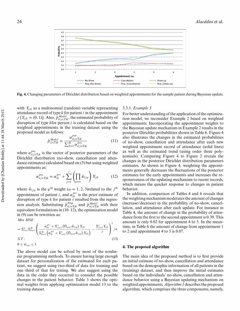
Fig. 4. Changing parameters of Dirichlet distribution based on weighted appointments for the sample patient during Bayesian update.
with Yi jk as a multinomial (random) variable representingattendance record of type k for patient i in the appointmentj(Yi jk = (0, 1)
). Also, p̂Model
i ( j∈T)k, the estimated probability ofdisruption of type kfor person i is calculated based on theweighted appointments in the training dataset using theproposed model as follows:
p̂Modeli j∈T)k =
αposi ( j∈T)k∑K
k=1 αposi ( j∈T)k
(11)
where αposi ( j∈T)k is the vector of posterior parameters of the
Dirichlet distribution (no-show, cancellation and atten-dance estimates) calculated based on (5) but using weightedappointments as:
αposi ( j∈T)k = α
priik +
t∑j=1
(∏ϕ∈ω
w̃i jϕ
)Yi jk (12)
where w̃i jϕ is the ϕth weight (ω = 1, 2, 3)related to the j th
appointment of patient i , and αpriik is the prior estimate of
disruption of type k for patient i resulted from the regres-sion analysis. Substituting p̂Emp
i ( j∈T)k and p̂Modeli ( j∈T)k with their
equivalent formulations in (10–12), the optimization modelin (9) can be rewritten as:Min MSE
= �ni=1�
Kk=1
⎛⎝ α
priik +�t
j=1
(�ϕ∈ωw̃i jϕ
)Yi jk
�Kk=1
(α
priik +�t
j=1
(�ϕ∈ωw̃i jϕ
)Yi jk
) − �tj=1Yi jk
t
⎞⎠
2
/n
S.T : (13)
0 ≤ w̃i jϕ ≤ 1
The above model can be solved by most of the nonlin-ear programming methods. To ensure having large enoughdataset for personalization of the estimated for each pa-tient, we suggest using two-third of data for training andone–third of that for testing. We also suggest using thedata in the order they occurred to consider the possiblechanges in the patient behavior. Table 5 shows the opti-mal weights from applying optimization model 13 to thetraining dataset.
3.3.1. Example 3For better understanding of the application of the optimiza-tion model, we reconsider Example 2 based on weightedappointments. Incorporating the appointment weights tothe Bayesian update mechanism in Example 2 results in theposterior Dirichlet probabilities shown in Table 6. Figure 4also illustrates the changes in the estimated probabilitiesof no-show, cancellation and attendance after each newweighted appointment record of attendance (solid lines)as well as the estimated trend (using order three poly-nomials). Comparing Figure 4 to Figure 2 reveals thechanges in the posterior Dirichlet distribution parametersestimates. As shown in Figure 4, weighting the appoint-ments generally decreases the fluctuations of the posteriorestimates for the early appointments and increases the re-sponsiveness of the updating mechanism to recent records,which means the quicker response to changes in patientbehavior.
In addition, comparison of Tables 4 and 6 reveals thatthe weighting mechanism moderates the amount of changes(increase/decrease) in the probability of no-show, cancel-lation, and attendance after each update. For instance inTable 4, the amount of change in the probability of atten-dance from the first to the second appointment is 0.39. Thisamount is only 0.02 for appointment 4 to 5. In the mean-time, in Table 6 the amount of change from appointment 1to 2 and appointment 4 to 5 is 0.07.
4. The proposed algorithm
The main idea of the proposed method is to first providean initial estimate of no-show, cancellation and attendancebased on the demographic information of all patients in the(training) dataset, and then improve the initial estimatesbased on the individuals’ no-show, cancellation and atten-dance behavior using a Bayesian updating mechanism onweighted appointments. Algorithm 1 describes the proposedalgorithm, which comprises the three components, namely,
Dow
nloa
ded
by [
Cha
ndan
Red
dy]
at 1
1:44
18
Mar
ch 2
015

A hybrid prediction model 25
multinomial logistic regression, Bayesian update mecha-nism, and the optimization procedure that is explained inthe previous section.
Algorithm 1: No-show and Cancellation Prediction Algorithm
Input: Training dataset(Xi j , Yi j
), Threshold parameter T
Output: Estimated no-show and cancellation probabilities
p̂Model , the Dirichlet distribution posterior parameters(α
posi j
),
Multinomial logistic regression estimated parameters B̂kProcedure:1: /∗ Logistic regression∗/2: B̂k← Estimate the parameters of multinomial logistic
regression in (3)3: p̂0
ik
(Yi = 1, 2, 3|Xi j
)← F(
Xi j , B̂k
)4: α
priik ← p̂0
ik5: /∗Weight optimization∗/
6: p̂Empi ( j∈T)k =
∑tj=1 Yi jk
t7: w̃i jϕ ← MinMSE =
n∑i=1
K∑k=1
(α
priik +
∑tj=1(
∏ϕ∈ω w̃i jϕ)Yi jk∑K
k=1(α priik +
∑tj=1(
∏ϕ∈ω w̃i jϕ)Yi jk)
−∑t
j=v1+1 Yi jk
t
)2
/n Subjectto0 ≤ w̃i jϕ ≤ 18: /∗Bayesian update ∗/
9: αposi ( j∈T)k = α
priik +
t∑j=1
(∏ϕ∈ω
w̃i jϕ
)Yi jk
10: p̂Modeli ( j∈T)k =
αposi ( j∈T)k∑K
k=1 αposi ( j∈T)k
11: Return p̂Model
In the first component (lines 1 to 3), based onthe training dataset consisting of individuals’ personalinformation(DG I ), (such as gender, marital status, etc.) andtheir sequence of appointment information (e.g. previousattendance records (DNR)), a multinomial logistic regres-
sion model F(
Xi j , B̂)
is formulated (line 2). Then, using
logistic regression, an initial estimate of no-show, cancella-tion and attendance probabilities are calculated, given byp̂0
ik
(Yi = 1, 2, 3|Xi j
)(line 3). This estimate
(p̂0
ik
)is used as
the prior of Bayesian update procedure(α
priik
)in the second
and third components (line 4). As discussed in Section 2,logistic regression bundles the information of the completepopulation together and finds a reliable initial estimate ofno-show ( p̂0
ik).In the second component (lines 5 to 7), which is interlaced
with the third component, the empirical rate of no-show,cancellation and attendance is calculated (Line 6). Then,an optimization model is used to find the optimal value ofa set of weighting factors (related to appointment recency,occurrence on non-working days and clinic type), whichminimizes the sum of squared differences in the predictionsform model (using weighted appointments) and empiricalestimates of no-show, cancellation and attendance in (Line7). As discussed in Section 3.3, the main purpose of weight-
ing the appointments (in Bayesian update) is to increase theinformation content of data to improve the prediction abil-ity of no-show and cancellation.
In the third component, using the weighted attendancerecord of each person (
∏ϕ∈ω
w̃i jϕ)Yi jk, the posterior param-
eters αPosi jk and posterior probability of attendance p̂Model
i jkis calculated (lines 9 and 10). As discussed in Section 2,the reason that Bayesian update procedure is applied tothe output of logistic regression is that, typically, regres-sion models cannot consider individual patient’s behavior.Also, updating the regression parameters based on newdata records is both difficult and only marginally effective(especially when the model is already constructed on a hugedataset) in comparison to the Bayesian update.
In practice, when the database of patient’s informationis large, once Algorithm 1 is built and executed, only line9 and 10 of the algorithm is required to be executed againupon receiving new data for a subset of patients. The reasonis because the logistic regression and weight optimizationparts are already built based on large amount of data andthe estimates are confident. Nonetheless, at the individualpatient level, the number of records may not be enough,or the patient may change her/his behavior. Therefore, theBayesian update (Line 0 to 10) based on weighted appoint-ments is used to further personalize the estimates. If thesize of the database is not large, the clinic may need torun the whole algorithm whenever the size of newly addeddata is comparable to the size of original dataset, e.g., everymonth.
5. Experimental results
In this section, we compare the performance of theproposed model with different population-based andindividual-based algorithms based on the dataset collectedat the Veteran Affairs (VA) Medical Center in Detroit us-ing time-wise analysis. For this purpose, the training andtesting data are constructed as follows: appointments thatoccurred before 2/1/2010 have been used for training andappointments after 2/1/2010 have been considered for test-ing. The main reason for selecting the above dates is to haveapproximately two-third of data records for training andthe rest of the data for testing.
5.1. Time-wise analysis
In this section, we compare the performance of theproposed model with a number of population-based,individual-based and adaptation algorithms using time-wise analysis. The methods used in our comparison alongwith their information are presented in Table 7.
Figure 5 illustrates the mean squared error (MSE) ofthe comparing methods. Based on the MSE measure, theproposed model outperforms other methods, while Box
Dow
nloa
ded
by [
Cha
ndan
Red
dy]
at 1
1:44
18
Mar
ch 2
015

26 Alaeddini et al.
Fig. 5. Mean Squared Error (MSE) of the comparing methods for time-wise analysis.
Fig. 6. ROC curves of the comparing methods for no-show prediction: (a) proposed method, (b) pure logistic regression, and (c) pureBayesian update.
Fig. 7. ROC curves of the comparing methods for cancellation prediction: (a) proposed method, (b) pure logistic regression, and (c)pure Bayesian update.
Dow
nloa
ded
by [
Cha
ndan
Red
dy]
at 1
1:44
18
Mar
ch 2
015

A hybrid prediction model 27
Fig. 8. Estimated versus empirical probability of appointment disruptions from the proposed approach over different patients: (a)no-show estimation, and (b) cancellation estimation.
Fig. 9. Estimated versus empirical probability of appointment disruptions from the pure multinomial logistic regression over differentpatients: (a) no-show estimation, and (b) cancellation estimation.
Dow
nloa
ded
by [
Cha
ndan
Red
dy]
at 1
1:44
18
Mar
ch 2
015
28 Alaeddini et al.
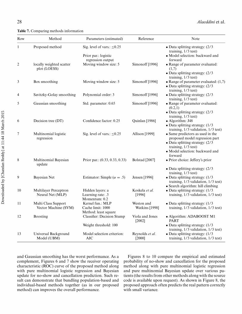
Table 7. Comparing methods information
Row Method Parameters (estimated) Reference Note
1 Proposed method Sig. level of vars.: ≤0.25 • Data splitting strategy: (2/3training, 1/3 test)
Prior par.: logisticregression output
•Model selection: backward andforward
2 locally weighted scatterplot (LOESS)
Moving window size: 5 Simonoff [1996] • Range of parameter evaluated:(1,7)• Data splitting strategy: (2/3
training, 1/3 test)3 Box smoothing Moving window size: 5 Simonoff [1996] •Range of parameter evaluated: (1,7)
• Data splitting strategy: (2/3training, 1/3 test)
4 Savitzky-Golay smoothing Polynomial order: 3 Simonoff [1996] • Data splitting strategy: (2/3training, 1/3 test)
5 Gaussian smoothing Std. parameter: 0.65 Simonoff [1996] • Range of parameter evaluated:(0.2,1)• Data splitting strategy: (2/3
training, 1/3 test)6 Decision tree (DT) Confidence factor: 0.25 Quinlan [1986] • Algorithm: J48
• Data splitting strategy: (1/3training, 1/3 validation, 1/3 test)
7 Multinomial logisticregression
Sig. level of vars.: ≤0.25 Allison [1999] • Same predictors as used in theproposed model regression part• Data splitting strategy: (2/3
training, 1/3 test)•Model selection: backward and
forward8 Multinomial Bayesian
updatePrior par.: (0.33, 0.33, 0.33) Bolstad [2007] • Prior choice: Jeffery’s prior
• Data splitting strategy: (2/3training, 1/3 test)
9 Bayesian Net Estimator: Simple (α = .5) Jensen [1996] • Data splitting strategy: (1/3training, 1/3 validation, 1/3 test)• Search algorithm: hill climbing
10 Multilayer PerceptronNeural Net (MLP)
Hidden layers: aLearning rate: .3Momentum: 0.2
Koskela et al.[1996]
• Data splitting strategy: (1/3training, 1/3 validation, 1/3 test)
11 Multi Class SupportVector Machine (SVM)
Kernel fun.: MLPCache limit: 1000Method: least square
Weston andWatkins [1998]
• Data splitting strategy: (1/3training, 1/3 validation, 1/3 test)
12 Boosting Classifier: Decision Stump Viola and Jones[2002]
• Algorithm: ADABOOST M1PART
Weight threshold: 100 • Data splitting strategy: (1/3training, 1/3 validation, 1/3 test)
13 Universal BackgroundModel (UBM)
Model selection criterion:AIC
Reynolds et al.[2000]
• Data splitting strategy: (1/3training, 1/3 validation, 1/3 test)
and Gaussian smoothing has the worst performance. As acomplement, Figures 6 and 7 show the receiver operatingcharacteristic (ROC) curve of the proposed method alongwith pure multinomial logistic regression and Bayesianupdate for no-show and cancellation prediction. Such re-sult can demonstrate that bundling population-based andindividual-based methods together (as in our proposedmethod) can improves the overall performance.
Figures 8 to 10 compare the empirical and estimatedprobability of no-show and cancellation for the proposedmethod along with pure multinomial logistic regressionand pure multinomial Bayesian update over various pa-tients (the results from other methods along with the sourcecode is available upon request). As shown in Figure 8, theproposed approach often predicts the real pattern correctlywith small variance.
Dow
nloa
ded
by [
Cha
ndan
Red
dy]
at 1
1:44
18
Mar
ch 2
015
A hybrid prediction model 29
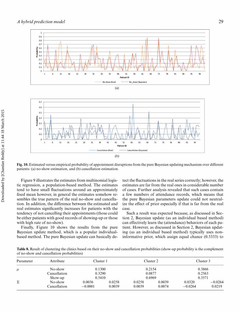
Fig. 10. Estimated versus empirical probability of appointment disruptions from the pure Bayesian updating mechanism over differentpatients: (a) no-show estimation, and (b) cancellation estimation.
Figure 9 illustrates the estimates from multinomial logis-tic regression, a population-based method. The estimatestend to have small fluctuations around an approximatelyfixed mean however, in general the estimates somehow re-sembles the true pattern of the real no-show and cancella-tion. In addition, the difference between the estimated andreal estimates significantly increases for patients with thetendency of not cancelling their appointments (those couldbe either patients with good records of showing-up or thosewith high rate of no-show).
Finally, Figure 10 shows the results from the pureBayesian update method, which is a popular individual-based method. The pure Bayesian update can basically de-
tect the fluctuations in the real series correctly; however, theestimates are far from the real ones in considerable numberof cases. Further analysis revealed that such cases containa few numbers of attendance records, which means thatthe pure Bayesian parameters update could not neutral-ize the effect of prior especially if that is far from the realcase.
Such a result was expected because, as discussed in Sec-tion 2, Bayesian update (as an individual based method)can effectively learn the (attendance) behaviors of each pa-tient. However, as discussed in Section 2, Bayesian updat-ing (as an individual based method) typically uses non-informative prior, which assign equal chance (0.3333) to
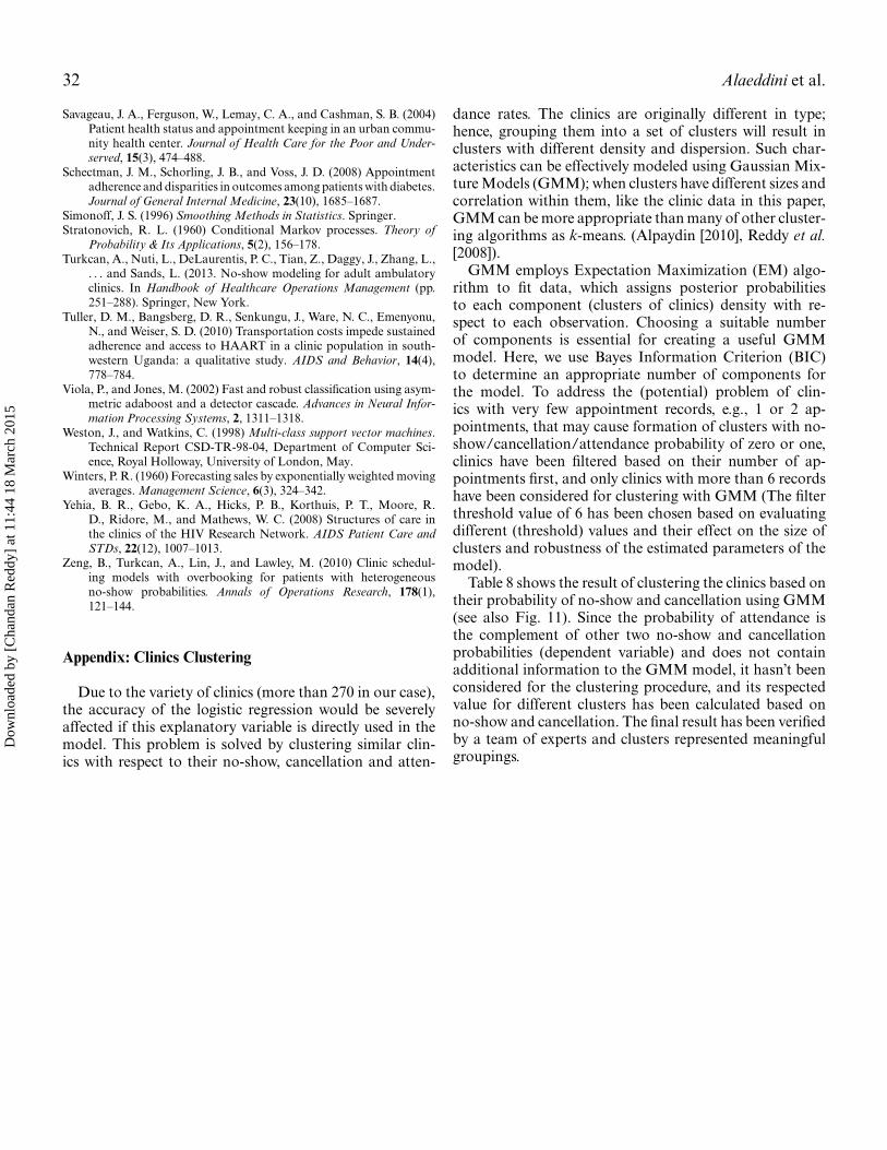
Table 8. Result of clustering the clinics based on their no-show and cancellation probabilities (show-up probability is the complementof no-show and cancellation probabilities)
Parameter Attribute Cluster 1 Cluster 2 Cluster 3
μ No-show 0.1300 0.2154 0.3866Cancellation 0.3290 0.0877 0.2563
Show-up 0.5410 0.6969 0.3571� No-show 0.0036 0.0258 0.0258 0.0039 0.0320 −0.0264
Cancellation −0.0001 0.0039 0.0039 0.0074 −0.0264 0.0219
Dow
nloa
ded
by [
Cha
ndan
Red
dy]
at 1
1:44
18
Mar
ch 2
015

30 Alaeddini et al.
Fig. 11. The contour plot of the mixture of distributions forno-show and cancellation probabilities resulted from applyingGMM.
each of no-show, cancellation and attendance,and non-informative prior may not be an appropriate choice in manycases as shown in Figure 10.
In summary, the results from Figures 5 to 10 and theirfollow up discussions show applying Bayesian update (asan individual-based method) to the initial estimate resultedfrom multinomial logistic regression (as a population-basedmethod) works superior to Bayesian update and multi-nomial logistic regression applied individually, and com-pares favorably with population-based, individual-basedand adaptation algorithms.
6. Conclusion and future work
Efficacy of any scheduling system primarily depends on itsability to forecast and manage different types of disruptionsand uncertainties. In this paper, we developed a proba-bilistic model based on multinomial logistic regression andBayesian inference to estimate individuals’ probabilities ofno-show, cancellation and attendance in real-time. Basedon real patient data collected from a Veterans Affairs med-ical hospital, we evaluated and showed the effectiveness ofthe approach. We also modeled the effect of the appoint-ment date and clinic on the proposed method. Our ap-proach is computationally effective and easy to implement.Unlike population-based methods, it takes into accountthe individual behavior of patients. Also, in contrast to theindividual-based methods, it can utilize some valuable in-formation from the complete patient database to providereliable probabilistic estimates. The result of the proposedmethod can be used to develop more effective appointmentscheduling systems and more precise overbooking strate-gies to reduce the negative effect of no-shows and fill inappointment slots while maintaining short waiting times.
References
Adomavicius, G., and Tuzhilin, A. (2005) Toward the next generation ofrecommender systems: A survey of the state-of-the-art and possibleextensions. Knowledge and Data Engineering, IEEE Transactions on,17(6), 734–749.
Agresti, A. (2002) Categorical data analysis (Vol. 359). John Wiley andSons.
Aitchison, J. (1985). Practical Bayesian problems in simplex samplespaces. Bayesian Statistics, 2, 15–31.
Alaeddini, A., Yang, K., Reddy, C., and Yu, S. (2011) A probabilisticmodel for predicting the probability of no-show in hospital ap-pointments. Health Care Management Science, 14(2), 146–157.
Alafaireet, P., Houghton, H., Petroski, G., Gong, Y., and Savage, G. T.(2010) Toward determining the structure of psychiatric visit non-adherence. The Journal of Ambulatory Care Management, 33(2),108–116.
Allison, P. (1999) Logistic Regression Using SAS R©: Theory and Applica-tion. SAS Publishing.
Alpaydin, E. (2004) Introduction to Machine Learning. MIT Press.Baldi, P., Brunak, S., Chauvin, Y., Andersen, C. A., and Nielsen, H. (2000)
Assessing the accuracy of prediction algorithms for classification:an overview. Bioinformatics, 16(5), 412–424.
Barron, W. M. (1980) Failed appointments. Who misses them, why theyare missed, and what can be done. Primary Care, 7(4), 563–574.
Bech, M. (2005) The economics of non-attendance and the expected effectof charging a fine on non-attendees. Health Policy, 74(2), 181–191.
Bigby, J., Pappius, E., Cook, E. F., and Goldman, L. (1984) Medical con-sequences of missed appointments. Archives of Internal Medicine,144(6), 1163–1166.
Bloomfield, P. (2004) Fourier Analysis of Time Series: An Introduction.John Wiley & Sons.
Bolstad, W. M. (2007) Introduction to Bayesian Statistics. John Wiley &Sons.
Bowser, D. M., Utz, S., Glick, D., and Harmon, R. (2010) A systematic re-view of the relationship of diabetes mellitus, depression, and missedappointments in a low-income uninsured population. Archives ofPsychiatric Nursing, 24(5), 317–329.
Brockwell, P. J., and Davis, R. A. (2009) Time Series: Theory and Methods.Springer.
Can, S., Macfarlane, T., and O’Brien, K. D. (2003) The use of postalreminders to reduce non-attendance at an orthodontic clinic: a ran-domised controlled trial. British Dental Journal, 195(4), 199–201.
Cayirli, T., and Veral, E. (2003) Outpatient scheduling in health care: areview of literature. Production and Operations Management, 12(4),519–549.
Cayirli, T., Veral, E., and Rosen, H. (2006) Designing appointmentscheduling systems for ambulatory care services. Health Care Man-agement Science, 9(1), 47–58.
Cayirli, T., Veral, E., and Rosen, H. (2008) Assessment of patient clas-sification in appointment system design. Production and OperationsManagement, 17(3), 338–353.
Chakraborty, S., Muthuraman, K., and Lawley, M. (2010) Sequentialclinical scheduling with patient no-shows and general service timedistributions. IIE Transactions, 42(5), 354–366.
Chatfield, C. (2013) The Analysis of Time Series: An Introduction. CRCPress.
Cleveland, W. S. (1993) Visualizing Data. Hobart Press.Cohen, A. D., Dreiher, J., Vardy, D. A., and Weitzman, D. (2008) Nonat-
tendance in a dermatology clinic–a large sample analysis. Journalof the European Academy of Dermatology and Venereology, 22(10),1178–1183.
Cote, M. J. (1999) Patient flow and resource utilization in an outpatientclinic. Socio-Economic Planning Sciences, 33(3), 231–245.
Corfield, L., Schizas, A., Williams, A., and Noorani, A. (2008) Non-attendance at the colorectal clinic: a prospective audit. Annals of theRoyal College of Surgeons of England, 90(5), 377.
Dow
nloa
ded
by [
Cha
ndan
Red
dy]
at 1
1:44
18
Mar
ch 2
015

A hybrid prediction model 31
Daggy, J., Lawley, M., Willis, D., Thayer, D., Suelzer, C., DeLaurentis,P. C., . . . and Sands, L. (2010) Using no-show modeling to improveclinic performance. Health Informatics Journal, 16(4), 246–259.
Denhaerynck, K., Manhaeve, D., Dobbels, F., Garzoni, D., Nolte, C.,and De Geest, S. (2007) Prevalence and consequences of nonadher-ence to hemodialysis regimens. American Journal of Critical Care,16(3), 222–235.
Dove, H. G., and Schneider, K. C. (1981) The usefulness of patients’ in-dividual characteristics in predicting no-shows in outpatient clinics.Medical Care, 19(7), 734–740.
Evans, M., Hastings, N., and Peacock, B. (2000) Statistical DistributionsWiley.
Fischman, D. (2010) Applying lean six sigma methodologies to improveefficiency, timeliness of care, and quality of care in an internalmedicine residency clinic. Quality Management in Healthcare, 19(3),201–210.
Forster, J. J., and Skene, A. M. (1994) Calculation of marginal densitiesfor parameters of multinomial distributions. Statistics and Comput-ing, 4(4), 279–286.
Gany, F., Ramirez, J., Chen, S., and Leng, J. C. (2011) Targeting socialand economic correlates of cancer treatment appointment keepingamong immigrant Chinese patients. Journal of Urban Health, 88(1),98–103.
Garuda, S. R., Javalgi, R. G., and Talluri, V. S. (1998) Tackling no-showbehavior: a market-driven approach. Health Marketing Quarterly,15(4), 25–44.
George, A., and Rubin, G. (2003) Non-attendance in general practice: asystematic review and its implications for access to primary healthcare. Family Practice, 20(2), 178–184.
Glowacka, K. J., Henry, R. M., and May, J. H. (2009) A hybrid datamining/simulation approach for modeling outpatient no-shows inclinic scheduling. Journal of the Operational Research Society, 60,1056–1068.
Goutis, C. (1993) Bayesian estimation methods for contingency tables.Journal of the Italian Statistical Society, 2(1), 35–54.
Gupta, D., and Denton, B. (2008). Appointment scheduling inhealth care: Challenges and opportunities. IIE Transactions, 40(9),800–819.
Guse, C. E., Richardson, L., Carle, M., and Schmidt, K. (2003) Theeffect of exit-interview patient education on no-show rates at a fam-ily practice residency clinic. The Journal of the American Board ofFamily Practice, 16(5), 399–404.
Hardy, K. J., O’Brien, S. V., and Furlong, N. J. (2001) Quality improve-ment report: Information given to patients before appointments andits effect on non-attendance rate. BMJ: British Medical Journal,323(7324), 1298.
Hassin, R., and Mendel, S. (2008) Scheduling arrivals to queues: A single-server model with no-shows. Management Science, 54(3), 565–572.
Hilbe, J. M. (2009) Logistic Regression Models. CRC Press, Boca Raton,FL.
Hixon, A. L., Chapman, R. W., and Nuovo, J. (1999) Failure to keepclinic appointments: implications for residency education and pro-ductivity. Family Medicine-Kansas City, 31, 627–630.
Ho, C. J., and Lau, H. S. (1992) Minimizing total cost in schedulingoutpatient appointments. Management Science, 38(12), 1750–1764.
Jensen, F. V. (1996) An Introduction to Bayesian Networks (Vol. 210).UCL Press, London.
Kopach, R., DeLaurentis, P. C., Lawley, M., Muthuraman, K., Ozsen, L.,Rardin, R., . . . and Willis, D. (2007) Effects of clinical characteris-tics on successful open access scheduling. Health Care ManagementScience, 10(2), 111–124.
Kotsiantis, S. B. (2007) Supervised machine learning: a review of classi-fication techniques. Informatica, 31(3), 03505596.
Koskela, T., Lehtokangas, M., Saarinen, J., and Kaski, K. (1996, Septem-ber). Time series prediction with multilayer perceptron, FIR andElman neural networks. In Proceedings of the World Congress onNeural Networks (pp. 491–496).
LaGanga, L. R. (2011) Lean service operations: reflections and newdirections for capacity expansion in outpatient clinics. Journal ofOperations Management, 29(5), 422–433.
LaGanga, L. R., and Lawrence, S. R. (2007). Clinic overbooking toimprove patient access and increase provider productivity. DecisionSciences, 38(2), 251–276.
Lehmann, T. N. O., Aebi, A., Lehmann, D., Balandraux Olivet, M.,and Stalder, H. (2007) Missed appointments at a Swiss universityoutpatient clinic. Public Health, 121(10), 790–799.
Leonard, T. (1973) A Bayesian method for histograms. Biometrika, 60(2),297–308.
Liu, N., Ziya, S., and Kulkarni, V. G. (2010) Dynamic scheduling ofoutpatient appointments under patient no-shows and cancellations.Manufacturing and Service Operations Management, 12(2), 347–364.
Mitchell, A., and Selmes, T. (2007) A comparative survey of missed initialand follow-up appointments to psychiatric specialties in the UnitedKingdom. Psychiatric Services, 58(6), 868–871.
Moore, C. G., Wilson-Witherspoon, P., and Probst, J. C. (2001) Timeand money: effects of no-shows at a family practice residency clinic.Family Medicine-Kansas City, 33(7), 522–527.
Murphy, K., Edelstein, H., Smith, L., Clanon, K., Schweitzer, B.,Reynolds, L., and Wheeler, P. (2011) Treatment of HIV in out-patients with schizophrenia, schizoaffective disorder and bipolardisease at two county clinics. Community Mental Health Journal,47(6), 668–671.
Murray, M. M., and Tantau, C. (2000) Same-day appointments: explod-ing the access paradigm. Family Practice Management, 7(8), 45–45.
Muthuraman, K., and Lawley, M. (2008) A stochastic overbookingmodel for outpatient clinical scheduling with no-shows. IIE Trans-actions, 40(9), 820–837.
Neal, R. D., Hussain-Gambles, M., Allgar, V. L., Lawlor, D. A., andDempsey, O. (2005) Reasons for and consequences of missed ap-pointments in general practice in the UK: questionnaire survey andprospective review of medical records. BMC Family Practice, 6(1),47.
Obialo, C. I., Bashir, K., Goring, S., Robinson, B., Quarshie, A., Al-Mahmoud, A., and Alexander-Squires, J. (2008). Dialysis “no-show” on Saturdays: Implications of the weekly hemodialysis sched-ules on nonadherence and outcomes. Journal of the National MedicalAssociation, 100(4), 412–419.
O’Brien, S. M., and Dunson, D. B. (2004) Bayesian multivariate logisticregression. Biometrics, 60(3), 739–746.
Park, W. B., Kim, J. Y., Kim, S. H., Kim, H. B., Kim, N. J., Oh, M. D.,and Choe, K. W. (2008) Self-reported reasons among HIV-infectedpatients for missing clinic appointments. International Journal ofSTD & AIDS, 19(2), 125–126.
Quinlan, J. R. (1986) Induction of decision trees. Machine Learning, 1(1),81–106.
Reddy, C. K., Chiang, H. D., and Rajaratnam, B. (2008) Trust-tech-based expectation maximization for learning finite mixture models.Pattern Analysis and Machine Intelligence, IEEE Transactions on,30(7), 1146–1157.
Reynolds, D. A., Quatieri, T. F., and Dunn, R. B. (2000) Speaker ver-ification using adapted Gaussian mixture models. Digital SignalProcessing, 10(1), 19–41.
Richards F. J. (1959) A flexible growth function for empirical use. Journalof Experimental Botany, 10(2), 290–301.
Rowett, M., Reda, S., and Makhoul, S. (2010) Prompts to encour-age appointment attendance for people with serious mental illness.Schizophrenia Bulletin, 36(5), 910–911.
Rust, C. T., Gallups, N. H., Clark, W. S., Jones, D. S., and Wilcox, W. D.(1995).Patient appointment failures in pediatric resident continuityclinics. Archives of Pediatrics & Adolescent Medicine, 149(6), 693.
Sarnquist, C. C., Soni, S., Hwang, H., Topol, B. B., Mutima, S., andMaldonado, Y. A. (2011) Rural HIV-infected women’s access tomedical care: ongoing needs in California. AIDS Care, 23(7),792–796.
Dow
nloa
ded
by [
Cha
ndan
Red
dy]
at 1
1:44
18
Mar
ch 2
015
32 Alaeddini et al.
Savageau, J. A., Ferguson, W., Lemay, C. A., and Cashman, S. B. (2004)Patient health status and appointment keeping in an urban commu-nity health center. Journal of Health Care for the Poor and Under-served, 15(3), 474–488.
Schectman, J. M., Schorling, J. B., and Voss, J. D. (2008) Appointmentadherence and disparities in outcomes among patients with diabetes.Journal of General Internal Medicine, 23(10), 1685–1687.
Simonoff, J. S. (1996) Smoothing Methods in Statistics. Springer.Stratonovich, R. L. (1960) Conditional Markov processes. Theory of
Probability & Its Applications, 5(2), 156–178.Turkcan, A., Nuti, L., DeLaurentis, P. C., Tian, Z., Daggy, J., Zhang, L.,
. . . and Sands, L. (2013. No-show modeling for adult ambulatoryclinics. In Handbook of Healthcare Operations Management (pp.251–288). Springer, New York.
Tuller, D. M., Bangsberg, D. R., Senkungu, J., Ware, N. C., Emenyonu,N., and Weiser, S. D. (2010) Transportation costs impede sustainedadherence and access to HAART in a clinic population in south-western Uganda: a qualitative study. AIDS and Behavior, 14(4),778–784.
Viola, P., and Jones, M. (2002) Fast and robust classification using asym-metric adaboost and a detector cascade. Advances in Neural Infor-mation Processing Systems, 2, 1311–1318.
Weston, J., and Watkins, C. (1998) Multi-class support vector machines.Technical Report CSD-TR-98-04, Department of Computer Sci-ence, Royal Holloway, University of London, May.
Winters, P. R. (1960) Forecasting sales by exponentially weighted movingaverages. Management Science, 6(3), 324–342.
Yehia, B. R., Gebo, K. A., Hicks, P. B., Korthuis, P. T., Moore, R.D., Ridore, M., and Mathews, W. C. (2008) Structures of care inthe clinics of the HIV Research Network. AIDS Patient Care andSTDs, 22(12), 1007–1013.
Zeng, B., Turkcan, A., Lin, J., and Lawley, M. (2010) Clinic schedul-ing models with overbooking for patients with heterogeneousno-show probabilities. Annals of Operations Research, 178(1),121–144.
Appendix: Clinics Clustering
Due to the variety of clinics (more than 270 in our case),the accuracy of the logistic regression would be severelyaffected if this explanatory variable is directly used in themodel. This problem is solved by clustering similar clin-ics with respect to their no-show, cancellation and atten-
dance rates. The clinics are originally different in type;hence, grouping them into a set of clusters will result inclusters with different density and dispersion. Such char-acteristics can be effectively modeled using Gaussian Mix-ture Models (GMM); when clusters have different sizes andcorrelation within them, like the clinic data in this paper,GMM can be more appropriate than many of other cluster-ing algorithms as k-means. (Alpaydin [2010], Reddy et al.[2008]).
GMM employs Expectation Maximization (EM) algo-rithm to fit data, which assigns posterior probabilitiesto each component (clusters of clinics) density with re-spect to each observation. Choosing a suitable numberof components is essential for creating a useful GMMmodel. Here, we use Bayes Information Criterion (BIC)to determine an appropriate number of components forthe model. To address the (potential) problem of clin-ics with very few appointment records, e.g., 1 or 2 ap-pointments, that may cause formation of clusters with no-show/cancellation/attendance probability of zero or one,clinics have been filtered based on their number of ap-pointments first, and only clinics with more than 6 recordshave been considered for clustering with GMM (The filterthreshold value of 6 has been chosen based on evaluatingdifferent (threshold) values and their effect on the size ofclusters and robustness of the estimated parameters of themodel).
Table 8 shows the result of clustering the clinics based ontheir probability of no-show and cancellation using GMM(see also Fig. 11). Since the probability of attendance isthe complement of other two no-show and cancellationprobabilities (dependent variable) and does not containadditional information to the GMM model, it hasn’t beenconsidered for the clustering procedure, and its respectedvalue for different clusters has been calculated based onno-show and cancellation. The final result has been verifiedby a team of experts and clusters represented meaningfulgroupings.
Dow
nloa
ded
by [
Cha
ndan
Red
dy]
at 1
1:44
18
Mar
ch 2
015