Embed Size (px)
Citation preview
Int. Journal of Math. Analysis, Vol. 6, 2012, no. 60, 2963 - 2976
A Hybrid Method Based on Particle Swarm Optimization
and Nonmonotone Spectral Gradient Method for
Unconstrained Optimization Problem
Halima LAKHBAB1 and Souad EL BERNOUSSI2
1,2Laboratory of Mathematics Informatics and ApplicationsFaculty of Sciences Rabat
Mohammed V University, Agdal1 [email protected], 2 [email protected]
Abstract
In the present work, the best characteristics of the Particle Swarm
Optimization (PSO) are combined with the good local search character-
istics of the Nonmonotone Spectral Gradient (NSG) to develop a novel
hybrid algorithm based on PSO algorithm; the proposed algorithm is
called PSO-NSG. The basic idea of PSO-NSG is to use the NSG algo-
rithm after each l iterations of the PSO, where l is a pre�xed integer.
The novel algorithm can be widely applied to a class of global opti-
mization problems for continuously di�erentiable functions. Simulations
for benchmark test functions and also for Sensor Network Localization
problem (SNLP) illustrate the robustness and e�ciency of the method
presented.
Mathematics Subject Classi�cation: 90C30, 90C59
Keywords: Nonmonotone spectral gradient method, particle swarm opti-mization, sensor network localization problem
1 Introduction
We consider the unconstrained minimization problem
minx∈Rn
f(x) (1)
where f : Rn −→ R is a continuously di�erentiable function de�ned on Rn.Several deterministic and stochastic optimization algorithms have been de-
veloped over last few decades for solving problem (1). Among them, we have
2964 H. LAKHBAB and S. EL BERNOUSSI
many metaheuristic methods like PSO that is a recent addition to the list ofglobal search methods. The system is initializing to be a series of stochasticsolutions, and search optimal value through iterations. Particles in the solu-tion space carry out search by following the optimal particle. PSO has receivedincreasing interest from the optimization community due to its simplicity inimplementation and its inexpensive computational overhead. However, PSOhas premature convergence, especially in complex multimodal functions.
Another di�erent type of methods that deal with the problem (1) arethe gradient-based algorithms like the nonmonotone spectral gradient (NSG)methods, in which a nonmonotone line search strategy is combined with thespectral gradient choice of steplength to accelerate the convergence process.In this paper, a new hybrid PSO algorithm is proposed, which combines theadvantages of both PSO (that has a strong global-search ability) and NSG(that has a strong local search ability).
The rest part of the paper is organized as follows: Section 2 provides abrief introduction of the classical particle swarm optimization and nonmono-tone spectral gradient method. Detail description of the new hybrid methodPSO−NSG is presented in Section 3. In section 4 numerical experiences arepresented in the solution of some test problems and also in the solution ofthe sensor network localization problem. Finally, section 5 discuss the testconclusion and include some �nal comments.
2 PSO and NSG methods
2.1 PSO method
Particle Swarm Optimization (PSO) is a metaheuristic which is inspired bythe swarm intelligence of social creatures, which interact between them in or-der to achieve a common goal. PSO has wide range of applications in manyareas. PSO is initialized with a population (or a swarm) of random solutions,called particles where each particle has its own velocity. Particles spread inthe multi dimensional search space, representing a possible solution, with ve-locities which are dynamically adjusted according to their historical behaviors.Therefore, the particles have a tendency to �y toward a better region of searchspace over the course of search process. The basic PSO algorithm consistsof three steps, namely, generating particle's positions and velocities, velocityupdate, and �nally, position update. A particle changes its position from onemove (iteration) to another based on velocity updates. First, the positions, xik, and velocities, vik, of the initial swarm of particles are randomly generatedusing upper and lower bounds on the design variables values, in the secondstep, velocities and positions of all particles are updated to persuade them toachieve better objective or �tness values which are functions of the particles
A hybrid method 2965
current positions in the design space at time k. The �tness function value ofa particle determines which particle has the best global value in the currentswarm, pgk, and also determines the best position of each particle over time, pi,i.e. in current and all previous moves. The velocity update formula is givenby
vik+1 = χ(vik + φ1r1(pi − xik) + φ2r2(p
gk − x
ik)) (2)
The constriction coe�cient χ is due to Clerc and Kennedy [8] and serves tokeep velocities from exploding. The φ1 and φ2 are constants and r1 and r2 arerandom numbers uniformly distributed in [0, 1].
At the �nal step, PSO update the position by using (3).
xik+1 = xik + vik (3)
2.2 A Nonmonotone Spectral Gradient (NSG) method
The unconstrained minimization problem (1), where f : Rn −→ R is a con-tinuously di�erentiable function, has di�erent iterative methods to solve it: Ifxk denotes the current iterate, and if it is not a good estimator of the solutionx∗, a better one, xk+1 = xk − αkgk is required. Here gk is the gradient vectorof f at xk and the scalar αk , is the step length.
A variant of the steepest descent was proposed in [1], which referred to the'Barzilai and Borwein' (BB) algorithm, where the step length αk along thesteepest descent −gk is chosen as in the raliegh quotient
αk =sTk−1sk−1
sTk−1yk−1
where sk−1 = xk − xk−1 and yk−1 = gk − gk−1. This choice of step lengthrequires little computational work and greatly speeds up the convergence ofgradient methods.
Raydan in [2] has proved a global convergence of (BB) algorithm under anonmonotone line search.
In nonmonotone spectral gradient method, the iterate xk satis�es a non-monotone Armijo line search (using su�cient decrease parameter γ over thelast M steps),
f(xk+1) ≤ max0≤j≤min{k,M}
f(xk−j) + γ〈gk, xk+1 − xk〉 (4)
Here the function values are allowed to increase at some iterations. This typeof condition (4) was introduced by Grippo, Lampariello, and Lucidi [3] andsuccessfully applied to Newton's method for a set of test functions.
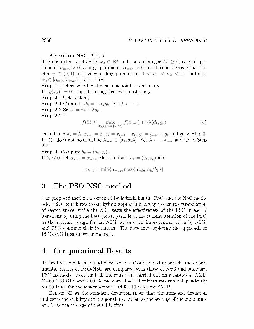
2966 H. LAKHBAB and S. EL BERNOUSSI
Algorithm NSG [2, 4, 5]The algorithm starts with x0 ∈ Rn and use an integer M ≥ 0; a small pa-rameter αmin > 0; a large parameter αmax > 0; a su�cient decrease param-eter γ ∈ (0, 1) and safeguarding parameters 0 < σ1 < σ2 < 1. Initially,α0 ∈ [αmin, αmax] is arbitrary.Step 1. Detect whether the current point is stationaryIf ‖g(xk)‖ = 0, stop, declaring that xk is stationary.Step 2. BacktrackingStep 2.1 Compute dk = −αkgk. Set λ←− 1.Step 2.2 Set x̃ = xk + λdk.Step 2.2 If
f(x̃) ≤ max0≤j≤min{k,M}
f(xk−j) + γλ〈dk, gk〉 (5)
then de�ne λk = λ, xk+1 = x̃, sk = xk+1−xk, yk = gk+1− gk and go to Step 3.If (5) does not hold, de�ne λnew ∈ [σ1, σ2λ]. Set λ ←− λnew and go to Step2.2.Step 3. Compute bk = 〈sk, yk〉.If bk ≤ 0, set αk+1 = αmax, else, compute ak = 〈sk, sk〉 and
αk+1 = min{αmax,max{αmin, ak/bk}}
3 The PSO-NSG method
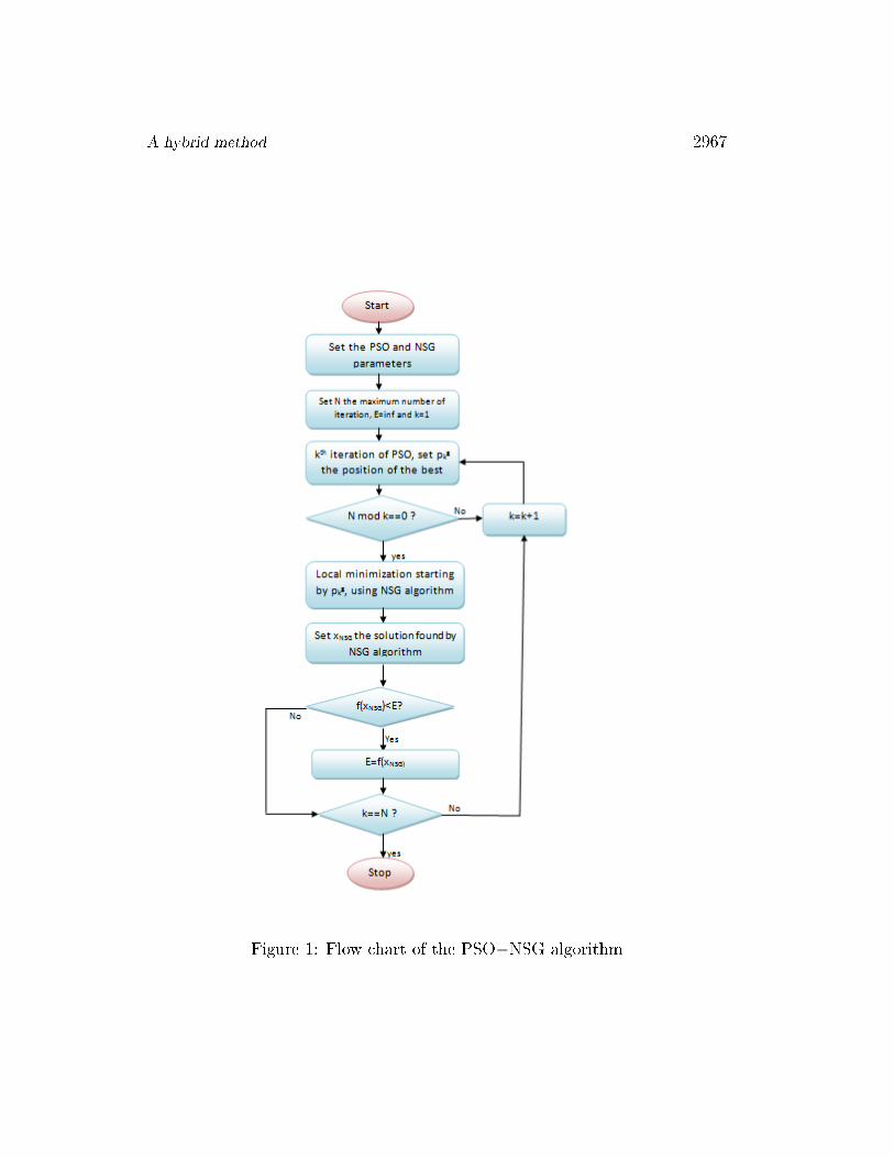
Our proposed method is obtained by hybridizing the PSO and the NSG meth-ods. PSO contributes to our hybrid approach in a way to ensure extrapolationof search space, while the NSG tests the e�ectiveness of the PSO in each literations by using the best global particle of the current iteration of the PSOas the starting design for the NSG, we save the improvement given by NSG,and PSO continue their iterations. The �owchart depicting the approach ofPSO-NSG is as shown in �gure 1.
4 Computational Results
To testify the e�ciency and e�ectiveness of our hybrid approach, the exper-imental results of PSO-NSG are compared with those of NSG and standardPSO methods. Note that all the runs were carried out on a laptop at AMDC−60 1.33 GHz and 2.00 Go memory. Each algorithm was run independentlyfor 20 trials for the test functions and for 10 trials for SNLP.
Denote SD as the standard deviation (note that the standard deviationindicates the stability of the algorithms), Mean as the average of the minimumsand T as the average of the CPU time.
A hybrid method 2967
Figure 1: Flow chart of the PSO−NSG algorithm
2968 H. LAKHBAB and S. EL BERNOUSSI
The PSO simulated in this study has a population of 100 particles; and themaximum number of generation is �xed at 100. The constriction coe�cient χis chosen as 0.7298; and the constant parameters are chosen as φ1 = φ2 = 2.05.And we �xe the radius of the box trust region to 0.01.
We implement the Algorithms PSO-NSG and NSG with the parametersdescribed in [5]: γ = 10−4, αmin = 10−30, αmax = 1030, σ1 = 0.1, σ2 =0.9 and α0 = 1/‖∇f(x0)‖∞.
We stopped the execution of the algorithms when the criterion ‖g(xk)‖∞ ≤etol was satis�ed or when Nmax iterations were completed without achievingconvergence. For the test functions we set etol = 10−6 andNmax = 5000 and forthe Sensor Network Localization Problem we setetol = 10−5 and Nmax = 50.
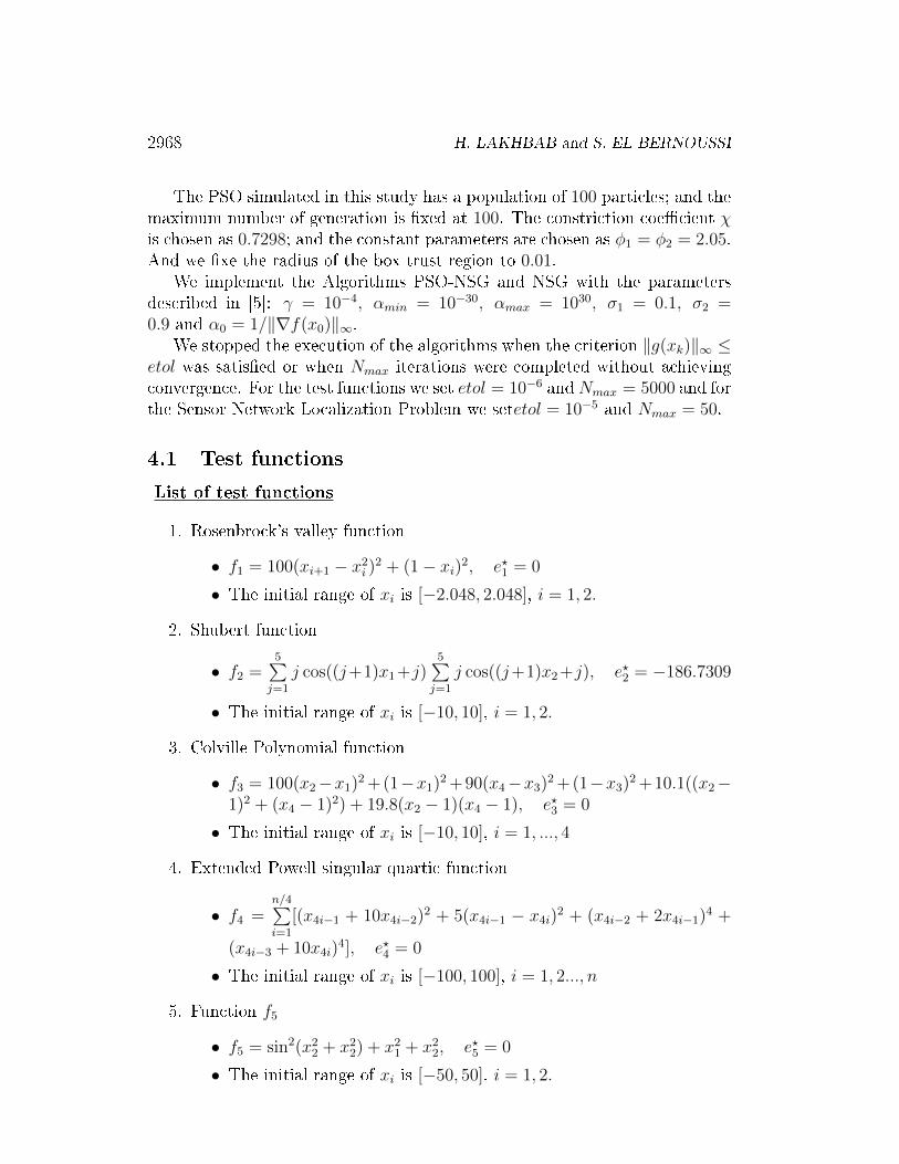
4.1 Test functions
List of test functions
1. Rosenbrock's valley function
• f1 = 100(xi+1 − x2i )2 + (1− xi)2, e?1 = 0
• The initial range of xi is [−2.048, 2.048], i = 1, 2.
2. Shubert function
• f2 =5∑
j=1
j cos((j+1)x1+j)5∑
j=1
j cos((j+1)x2+j), e?2 = −186.7309
• The initial range of xi is [−10, 10], i = 1, 2.
3. Colville Polynomial function
• f3 = 100(x2−x1)2 +(1−x1)2 +90(x4−x3)2 +(1−x3)2 +10.1((x2−1)2 + (x4 − 1)2) + 19.8(x2 − 1)(x4 − 1), e?3 = 0
• The initial range of xi is [−10, 10], i = 1, ..., 4
4. Extended Powell singular quartic function
• f4 =n/4∑i=1
[(x4i−1 + 10x4i−2)2 + 5(x4i−1 − x4i)
2 + (x4i−2 + 2x4i−1)4 +
(x4i−3 + 10x4i)4], e?4 = 0
• The initial range of xi is [−100, 100], i = 1, 2..., n
5. Function f5
• f5 = sin2(x22 + x22) + x21 + x22, e?5 = 0
• The initial range of xi is [−50, 50], i = 1, 2.
A hybrid method 2969
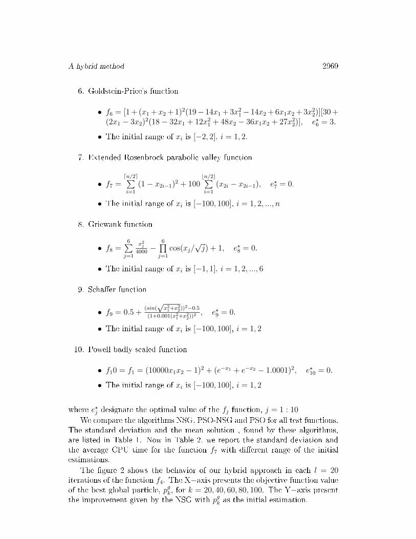
6. Goldstein-Price's function
• f6 = [1 + (x1 +x2 + 1)2(19− 14x1 + 3x21− 14x2 + 6x1x2 + 3x22)][30 +(2x1 − 3x2)
2(18− 32x1 + 12x21 + 48x2 − 36x1x2 + 27x22)], e?6 = 3.
• The initial range of xi is [−2, 2], i = 1, 2.
7. Extended Rosenbrock parabolic valley function
• f7 =dn/2e∑i=1
(1− x2i−1)2 + 100bn/2c∑i=1
(x2i − x2i−1), e?7 = 0.
• The initial range of xi is [−100, 100], i = 1, 2, ..., n
8. Griewank function
• f8 =6∑
j=1
x2j
4000−
6∏j=1
cos(xj/√j) + 1, e?8 = 0.
• The initial range of xi is [−1, 1], i = 1, 2, ..., 6
9. Scha�er function
• f9 = 0.5 +(sin(√
x21+x2
2))2−0.5
(1+0.001(x21+x2
2))2 , e?9 = 0.
• The initial range of xi is [−100, 100], i = 1, 2
10. Powell badly scaled function
• f10 = f1 = (10000x1x2 − 1)2 + (e−x1 + e−x2 − 1.0001)2, e?10 = 0.
• The initial range of xi is [−100, 100], i = 1, 2
where e?j designate the optimal value of the fj function, j = 1 : 10
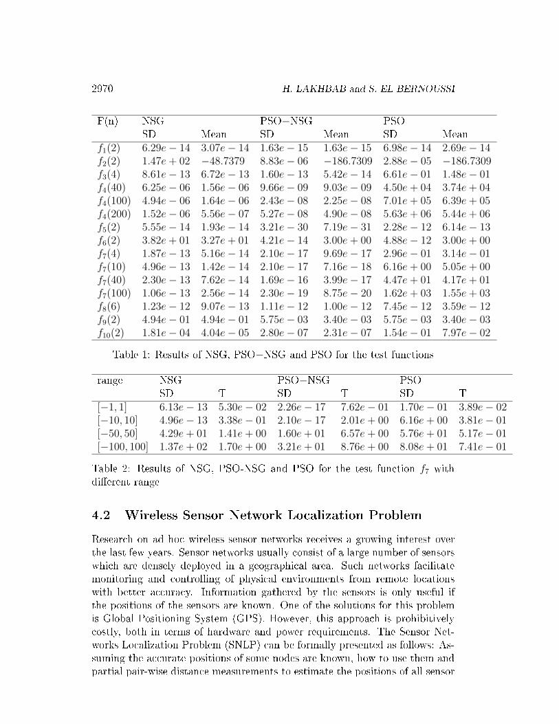
We compare the algorithms NSG, PSO-NSG and PSO for all test functions.The standard deviation and the mean solution , found by these algorithms,are listed in Table 1. Now in Table 2, we report the standard deviation andthe average CPU time for the function f7 with di�erent range of the initialestimations.
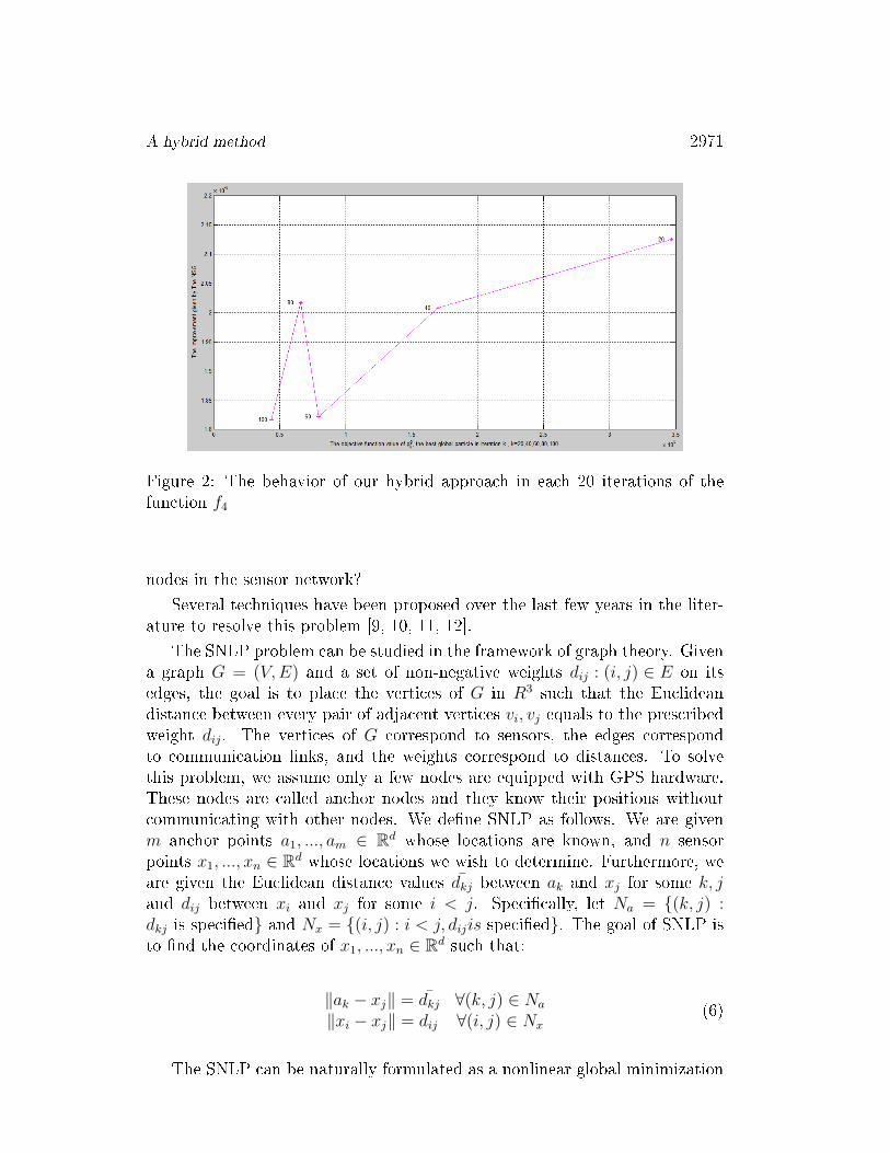
The �gure 2 shows the behavior of our hybrid approach in each l = 20iterations of the function f4. The X−axis presents the objective function valueof the best global particle, pgk, for k = 20, 40, 60, 80, 100. The Y−axis presentthe improvement given by the NSG with pgk as the initial estimation.
2970 H. LAKHBAB and S. EL BERNOUSSI
F(n) NSG PSO−NSG PSOSD Mean SD Mean SD Mean
f1(2) 6.29e− 14 3.07e− 14 1.63e− 15 1.63e− 15 6.98e− 14 2.69e− 14f2(2) 1.47e+ 02 −48.7379 8.83e− 06 −186.7309 2.88e− 05 −186.7309f3(4) 8.61e− 13 6.72e− 13 1.60e− 13 5.42e− 14 6.61e− 01 1.48e− 01f4(40) 6.25e− 06 1.56e− 06 9.66e− 09 9.03e− 09 4.50e+ 04 3.74e+ 04f4(100) 4.94e− 06 1.64e− 06 2.43e− 08 2.25e− 08 7.01e+ 05 6.39e+ 05f4(200) 1.52e− 06 5.56e− 07 5.27e− 08 4.90e− 08 5.63e+ 06 5.44e+ 06f5(2) 5.55e− 14 1.93e− 14 3.21e− 30 7.19e− 31 2.28e− 12 6.14e− 13f6(2) 3.82e+ 01 3.27e+ 01 4.21e− 14 3.00e+ 00 4.88e− 12 3.00e+ 00f7(4) 1.87e− 13 5.16e− 14 2.10e− 17 9.69e− 17 2.96e− 01 3.14e− 01f7(10) 4.96e− 13 1.42e− 14 2.10e− 17 7.16e− 18 6.16e+ 00 5.05e+ 00f7(40) 2.30e− 13 7.62e− 14 1.69e− 16 3.99e− 17 4.47e+ 01 4.17e+ 01f7(100) 1.06e− 13 2.56e− 14 2.30e− 19 8.75e− 20 1.62e+ 03 1.55e+ 03f8(6) 1.23e− 12 9.07e− 13 1.11e− 12 1.00e− 12 7.45e− 12 3.59e− 12f9(2) 4.94e− 01 4.94e− 01 5.75e− 03 3.40e− 03 5.75e− 03 3.40e− 03f10(2) 1.81e− 04 4.04e− 05 2.80e− 07 2.31e− 07 1.54e− 01 7.97e− 02
Table 1: Results of NSG, PSO−NSG and PSO for the test functions
range NSG PSO−NSG PSOSD T SD T SD T
[−1, 1] 6.13e− 13 5.30e− 02 2.26e− 17 7.62e− 01 1.70e− 01 3.89e− 02[−10, 10] 4.96e− 13 3.38e− 01 2.10e− 17 2.01e+ 00 6.16e+ 00 3.81e− 01[−50, 50] 4.29e+ 01 1.41e+ 00 1.60e+ 01 6.57e+ 00 5.76e+ 01 5.17e− 01[−100, 100] 1.37e+ 02 1.70e+ 00 3.21e+ 01 8.76e+ 00 8.08e+ 01 7.41e− 01
Table 2: Results of NSG, PSO-NSG and PSO for the test function f7 withdi�erent range
4.2 Wireless Sensor Network Localization Problem
Research on ad hoc wireless sensor networks receives a growing interest overthe last few years. Sensor networks usually consist of a large number of sensorswhich are densely deployed in a geographical area. Such networks facilitatemonitoring and controlling of physical environments from remote locationswith better accuracy. Information gathered by the sensors is only useful ifthe positions of the sensors are known. One of the solutions for this problemis Global Positioning System (GPS). However, this approach is prohibitivelycostly, both in terms of hardware and power requirements. The Sensor Net-works Localization Problem (SNLP) can be formally presented as follows: As-suming the accurate positions of some nodes are known, how to use them andpartial pair-wise distance measurements to estimate the positions of all sensor
A hybrid method 2971
Figure 2: The behavior of our hybrid approach in each 20 iterations of thefunction f4
nodes in the sensor network?
Several techniques have been proposed over the last few years in the liter-ature to resolve this problem [9, 10, 11, 12].
The SNLP problem can be studied in the framework of graph theory. Givena graph G = (V,E) and a set of non-negative weights dij : (i, j) ∈ E on itsedges, the goal is to place the vertices of G in R3 such that the Euclideandistance between every pair of adjacent vertices vi, vj equals to the prescribedweight dij. The vertices of G correspond to sensors, the edges correspondto communication links, and the weights correspond to distances. To solvethis problem, we assume only a few nodes are equipped with GPS hardware.These nodes are called anchor nodes and they know their positions withoutcommunicating with other nodes. We de�ne SNLP as follows. We are givenm anchor points a1, ..., am ∈ Rd whose locations are known, and n sensorpoints x1, ..., xn ∈ Rd whose locations we wish to determine. Furthermore, weare given the Euclidean distance values d̄kj between ak and xj for some k, jand dij between xi and xj for some i < j. Speci�cally, let Na = {(k, j) :dkj is speci�ed} and Nx = {(i, j) : i < j, dijis speci�ed}. The goal of SNLP isto �nd the coordinates of x1, ..., xn ∈ Rd such that:
‖ak − xj‖ = d̄kj ∀(k, j) ∈ Na
‖xi − xj‖ = dij ∀(i, j) ∈ Nx(6)
The SNLP can be naturally formulated as a nonlinear global minimization
2972 H. LAKHBAB and S. EL BERNOUSSI
problem, where the objective function is given by
f(x1, ..., xn) =∑
(i,j)∈Nx
((‖xi − xj‖ − dij)2 +∑
(j,k)∈Na
((‖xj − ak‖ − d̄jk)2
This function is everywhere in�nitely di�erentiable, and by using the factthat the ∇x‖x − b‖ = (x − b)/‖x − b‖ , if x 6= b, the gradient ∇jf of theobjective function f with respect to the xj is given by:
∇jf(x1, ..., xn) =∑
(i,j)∈Nx
(1−dij/‖xj−xi‖)(xj−xi)+∑
(j,k)∈Na
(1−d̄ij/‖xj−ak‖)(xj−ak)
It is easy to see that the 0 is the global minimum of f . Therefore, thestructure of a network can be determined by �nding the this minimum.
In the following , we give examples to demonstrate the potential of ourhybrid approach in solving the localization problem for ad hoc sensor networks.We randomly generate test problems by the function generateProblem of thesparse SDP solver SFSDP111 [13]. We consider three problems: S3A4, S50A5and S100A10 that consist of 3 sensors and 4 anchors, 50 sensors and 5 anchorsand 100 sensors and 10 anchors, respetively.
Table 3 show the results of NSG, PSO-NSG and PSO, for 10 runs witheach example. We report in this table the standard deviations and the meansolutions.
S3A4 S50A5 S100A10NSG PSO−NSG PSO NSG PSO−NSG PSO NSG PSO−NSG PSO
SD 1.58e− 10 1.20e− 10 1.26e− 10 0.2758 0.2511 2.4313 1.5604 1.1265 10.8834Mean 2.15e− 10 1.70e− 10 1.78e− 10 0.3660 0.3432 3.4345 2.0206 1.5566 15.3823
Table 3: Results of NSG, PSO-NSG and PSO for 3 examples of SNLP
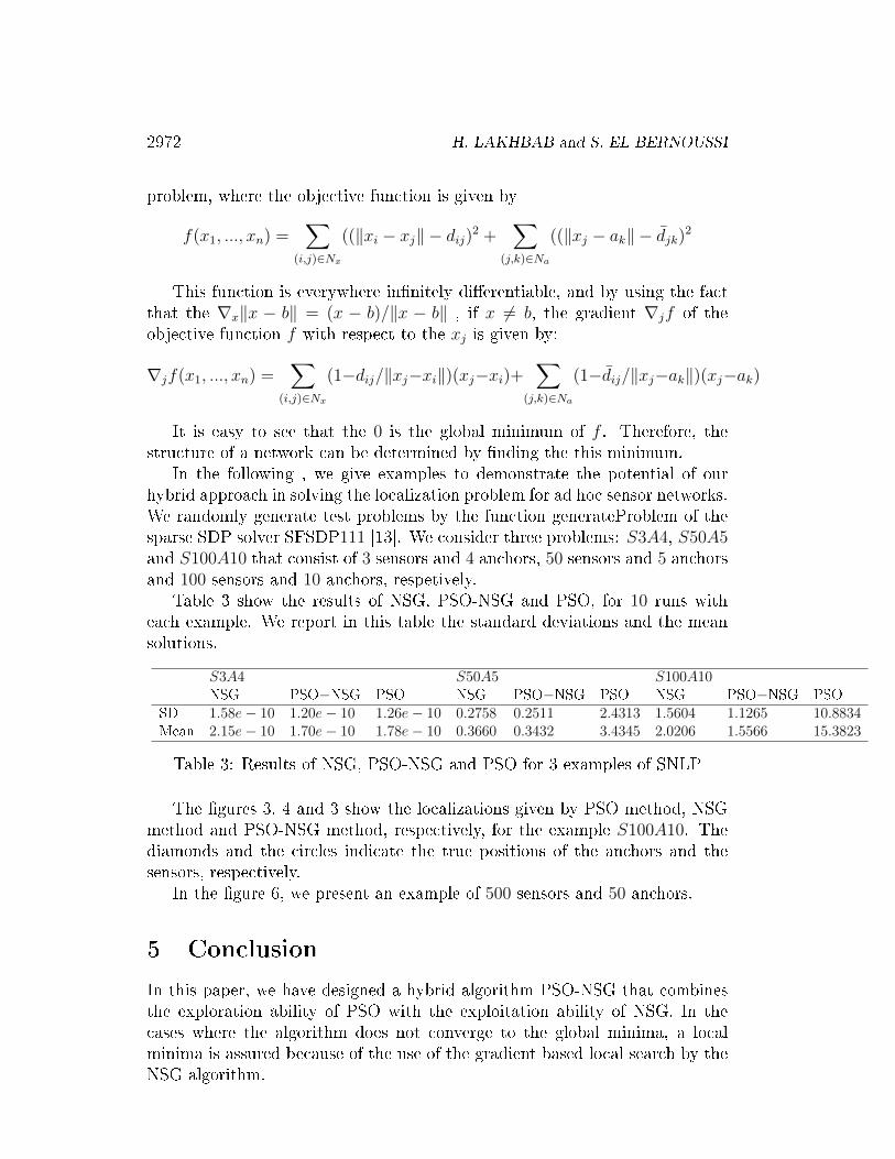
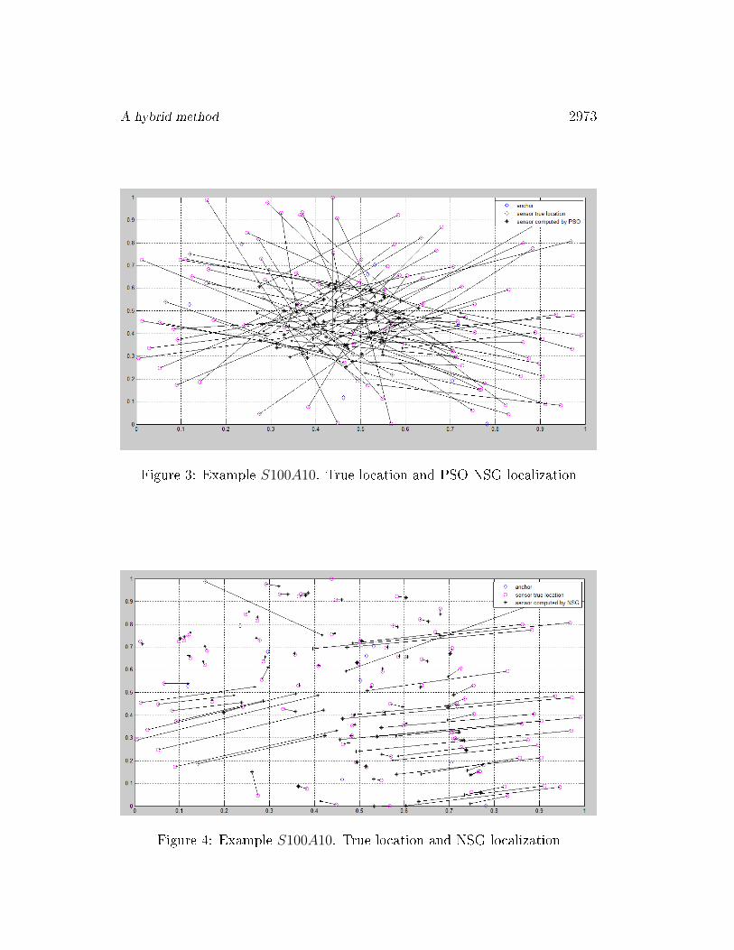
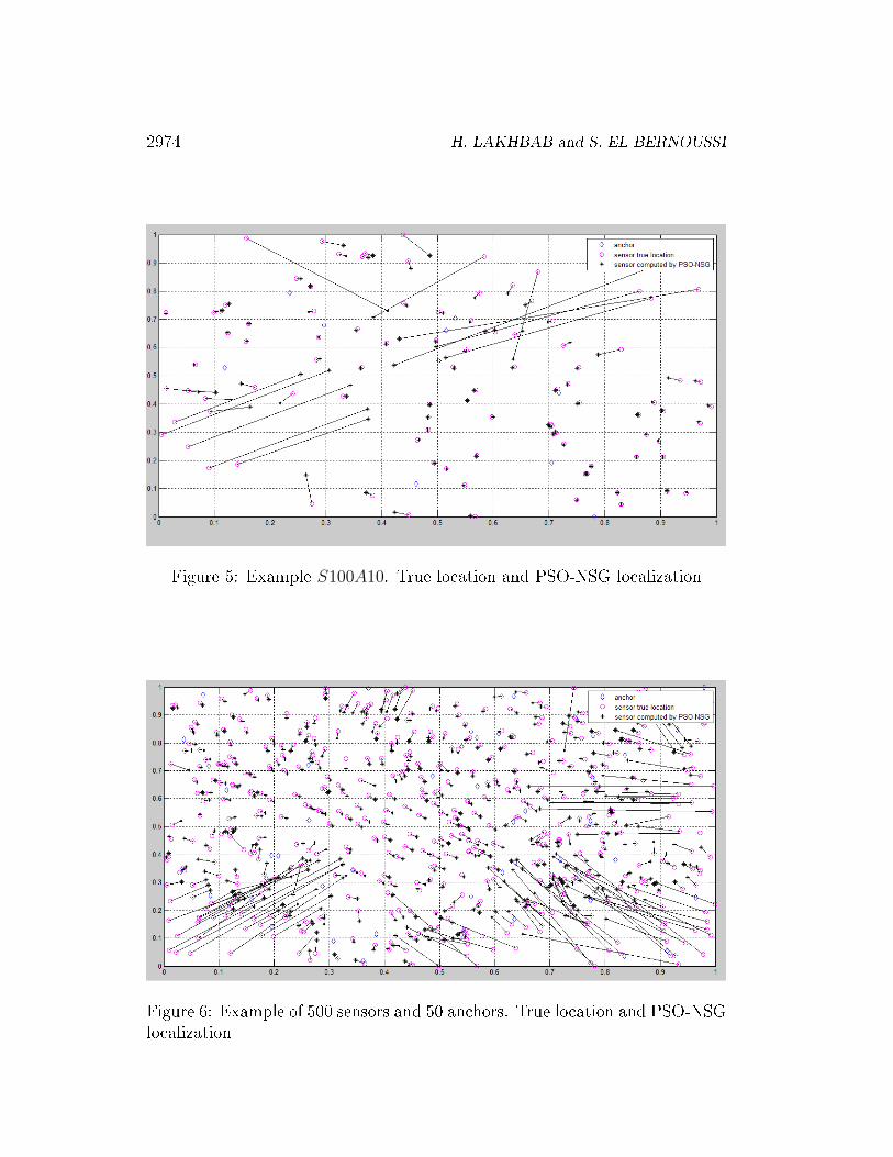
The �gures 3, 4 and 3 show the localizations given by PSO method, NSGmethod and PSO-NSG method, respectively, for the example S100A10. Thediamonds and the circles indicate the true positions of the anchors and thesensors, respectively.
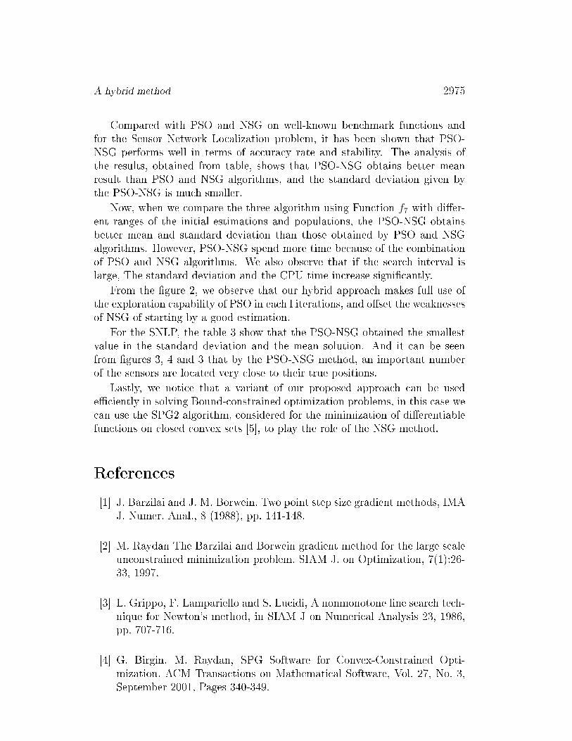
In the �gure 6, we present an example of 500 sensors and 50 anchors.
5 Conclusion
In this paper, we have designed a hybrid algorithm PSO-NSG that combinesthe exploration ability of PSO with the exploitation ability of NSG. In thecases where the algorithm does not converge to the global minima, a localminima is assured because of the use of the gradient based local search by theNSG algorithm.
A hybrid method 2973
Figure 3: Example S100A10. True location and PSO-NSG localization
Figure 4: Example S100A10. True location and NSG localization
2974 H. LAKHBAB and S. EL BERNOUSSI
Figure 5: Example S100A10. True location and PSO-NSG localization
Figure 6: Example of 500 sensors and 50 anchors. True location and PSO-NSGlocalization
A hybrid method 2975
Compared with PSO and NSG on well-known benchmark functions andfor the Sensor Network Localization problem, it has been shown that PSO-NSG performs well in terms of accuracy rate and stability. The analysis ofthe results, obtained from table, shows that PSO-NSG obtains better meanresult than PSO and NSG algorithms, and the standard deviation given bythe PSO-NSG is much smaller.
Now, when we compare the three algorithm using Function f7 with di�er-ent ranges of the initial estimations and populations, the PSO-NSG obtainsbetter mean and standard deviation than those obtained by PSO and NSGalgorithms. However, PSO-NSG spend more time because of the combinationof PSO and NSG algorithms. We also observe that if the search interval islarge, The standard deviation and the CPU time increase signi�cantly.
From the �gure 2, we observe that our hybrid approach makes full use ofthe exploration capability of PSO in each l iterations, and o�set the weaknessesof NSG of starting by a good estimation.
For the SNLP, the table 3 show that the PSO-NSG obtained the smallestvalue in the standard deviation and the mean solution. And it can be seenfrom �gures 3, 4 and 3 that by the PSO-NSG method, an important numberof the sensors are located very close to their true positions.
Lastly, we notice that a variant of our proposed approach can be usede�ciently in solving Bound-constrained optimization problems, in this case wecan use the SPG2 algorithm, considered for the minimization of di�erentiablefunctions on closed convex sets [5], to play the role of the NSG method.
References
[1] J. Barzilai and J. M. Borwein, Two point step size gradient methods, IMAJ. Numer. Anal., 8 (1988), pp. 141-148.
[2] M. Raydan The Barzilai and Borwein gradient method for the large scaleunconstrained minimization problem. SIAM J. on Optimization, 7(1):26-33, 1997.
[3] L. Grippo, F. Lampariello and S. Lucidi, A nonmonotone line search tech-nique for Newton's method, in SIAM J on Numerical Analysis 23, 1986,pp. 707-716.
[4] G. Birgin, M. Raydan, SPG Software for Convex-Constrained Opti-mization. ACM Transactions on Mathematical Software, Vol. 27, No. 3,September 2001, Pages 340-349.
2976 H. LAKHBAB and S. EL BERNOUSSI
[5] E.G. Birgin, J.M. Martínez, M.Raydan, Nonmonotone Spectral ProjectedGradient Methods on Convex Sets. SIAM J. on Optimization, 10(4):1196-1211, 2000.
[6] H. Lakhbab, S. El bernoussi and A. El harif, Energy Minimization of PointCharges on a Sphere with a Hybrid Approach. Applied MathematicalSciences, Vol. 6, 2012, no. 30, 1487- 1495.
[7] W. La Cruz and G. Noguera, Hybrid spectral gradient method for theunconstrained minimization problem. J Glob Optim (2009) 44:193-212.
[8] M. Clerc and J. Kennedy. (2002). The particle swarm: explosion, stability,and convergence in multi-dimensional complex space, IEEE Transactionson Evolutionary Computation, Vol. 6, pp. 58-73, 2002.
[9] T.-C. Liang, T.-C. Wang, and Y. Ye, A gradient search method to roundthe semide�nite programming relaxation solution for ad hoc wireless sen-sor network localization, technical report, Dept of Management Scienceand Engineering, Stanford University, August 2004.
[10] J. Aspnes, W. Whiteley, and Y. R. Yang, A theory of network localization,IEEE Trans. Mobile Comput., vol. 5, no. 12, pp. 1663-1678, 2006.
[11] P. Biswas, T. C. Lian, T. C. Wang, and Y. Ye, Semide�nite programmingbased algorithms for sensor network localization, ACM Trans. Sen. Netw.,vol. 2, no. 2, pp. 188-220, 2006.
[12] H. Lakhbab and S. El Bernoussi, Sensor Networks localization problemwith a new hybrid approach, in Proceedings of the ICMCS'2012: Inter-national Conference on Multimedia Computing and Systems, IEEE Con-ference, organized in Tangier (Morocco).
[13] S. Kim M. Kojima H. Waki and M. Yamashita, SFSDP: a Sparse Ver-sion of Full SemiDe�nite Programming Relaxation for Sensor NetworkLocalization Problems. August 2008, Revised July 2009. The packageSFSDP and this manual are available at http://www.is.titech.ac.jp/ ko-jima/SFSDP.
[14] N. Andrei, An Unconstrained Optimization Test Functions Collection,Advanced Modeling and Optimization, Volume 10, Number 1, 2008.
[15] TEST OPT Optimization of a Scalar Function Test Problems.
http://people.sc.fsu.edu/~jburkardt/m_src/test_opt/test_opt.html
Received: August, 2012