Contents lists available at ScienceDirect

Journal of Sound and Vibration

Journal of Sound and Vibration 333 (2014) 3625–3638

http://d0022-46

n CorrE-m

journal homepage: www.elsevier.com/locate/jsvi

A hybrid approach to reconstruct transient sound fieldbased on the free-field time reversal method andinterpolated time-domain equivalent source method

Siwei Pan, Weikang Jiang n

State Key Laboratory of Mechanical System and Vibration, Shanghai Jiao Tong University, 800 Dongchuan Road, Shanghai 200240, China

a r t i c l e i n f o

Article history:Received 22 August 2013Received in revised form21 March 2014Accepted 23 March 2014

Handling Editor: L. Huang

reversal focusing algorithm is performed to estimate the source locations on the source

Available online 22 April 2014

x.doi.org/10.1016/j.jsv.2014.03.0290X/& 2014 Elsevier Ltd. All rights reserved.

esponding author. Tel./fax: þ86 21 3420633ail address: wkjiang@sjtu.edu.cn (W. Jiang).

a b s t r a c t

A hybrid approach is presented in the current work, which reconstructs the transientsound field radiated from the two-dimensional sources with unknown locations and sizes,by combining the free-field time reversal method and the interpolated time-domainequivalent source method (TDESM). In the first step of the proposed method, the time

plane. And then, the interpolated TDESM is applied to reconstruct the transient soundfield on the reconstruction plane by assuming that the equivalent sources are located nearthe estimated source locations found in the previous step. The proposed technique, inprinciple, requires fewer microphones in the measurement since the equivalent sourcesare only placed in the vicinity of the ‘real’ sound sources. Reconstruction of the transientsound field radiated from the dual-planar-piston model is studied by numerical simula-tion for feasibility demonstration. A measurement of the sound fields radiated from twobaffled loudspeakers is performed in the anechoic chamber, which shows that a betterreconstruction result can be achieved by using the proposed hybrid scheme than theoriginal interpolated TDESM with relatively the same number of sampling channels.

& 2014 Elsevier Ltd. All rights reserved.

1. Introduction

Near-field acoustical holography (NAH) [1–3] is a well-known technique for the reconstruction of harmonic sound fields.However, the reconstructions of transient noises such as braking and riveting are often encountered in practice. To deal with thesetransient acoustic phenomena, some time-domain NAH (TNAH) methods have been developed. Most studies in the TNAH focus onthe plane wave superposition algorithm (PWSA), for example, Thomas et al. [4] proposed a so-called real-time near-field acousticholography (RT-NAH) method to continuously backward reconstruct the non-stationary acoustic fields on a projection plane byapplying a convolution between the instantaneous wavenumber spectrum and the inverse impulse response. Blais and Ross [5]made use of the Laplace transform to develop a Fourier transform-based transient NAH formulation, which was performed by usingthe direct and inverse time domain numerical Laplace transforms (NLTs). Zhang et al. [6] proposed a time-domain plane wavesuperposition method (TD-PWSM) to reconstruct non-stationary sound fields. This method replaces the two-dimensional spatial

2x820.

Nomenclature

a radius of circular pistons (m)c speed of sound (m/s)f0 fundamental frequency (Hz)fs sampling frequency (Hz)g(rm,rs;t) time-domain Green's function from rs to rm at

time thm(t) the impulse response from the source to the

mth measurement pointJ maximum source time stepM number of measurement points/sensorsN number of equivalent sourcesOutputTRM(t) output of time-reversal mirror (Pa)p(t) acoustic pressure (Pa)pCm(t) pressure on the reconstruction surface at time

t (Pa)pHm(t) pressure at the mth measurement point at

measurement time t (Pa)pm(t) signal measured at the mth measurement

point (Pa)pr reconstructed pressure on the reconstruction

surface (Pa)pt theoretical pressure on the reconstruction

surface (Pa)pTm(�t) time-reversed signal at the mth measurement

point with sampling length T (Pa)qn(τ) equivalent source strength at the source time

τ (Pa)qjn the nth equivalent source strength at the jth

source time (Pa)

RCmn distance of the mth reconstruction point fromthe nth equivalent source (m)

RHmn distance of the mth measurement point fromthe nth equivalent source (m)

Rms distance from rs to rm (m)rm the mth measurement pointrs focused positions(t) source signal (Pa)sT(t) initial source signal with length T (Pa)t measurement time (s)T sampling length (s)z(t) refocused signal (Pa)Δτ interval of the source time (s)τHmn source time corresponding to measurement

time t (s)τ source time (s)τCmn source time corresponding to reconstruction

time t (s)τ0 initial instant of the source time (s)τj the jth step source time (s)Φj(τ) a linear interpolation function

Abbreviations

RMSE root mean square error of reconstructionTR time-reversalTRM time-reversal mirrorTRS time-reversal sinkTDESM time-domain equivalent source methodGCV generalized cross-validation

S. Pan, W. Jiang / Journal of Sound and Vibration 333 (2014) 3625–36383626

fast Fourier transform (SFFT) that is generally employed in the TNAH with the direct discretization of double infinite integral in thewavenumber domain, theoretically avoiding some limitations associated with the SFFT. These PWSA-based TNAH methods can beused to reconstruct or predict the transient sound field, but they are restricted to the planar sources.

Wu et al. [7] derived a transient formulation of the Helmholtz equation least-squares (HELS) method to study thespherical sound sources subject to transient excitations. In his study, the inverse Laplace transform is used and calculated viathe residue theory. Bai et al. [8,9] proposed a near-field equivalence source imaging (NESI) technique to identify locationsand strengths of transient noise sources. The heart of this technique was to design the multichannel inverse filters. Lee et al.[10–12] developed a time-domain moving equivalent source method (TDMESM) to predict acoustic scattering in the timedomain efficiently. In the TDMESM, a linear interpolation function was used to discretize the strength of the equivalentsources in time and singular value decomposition (SVD) was used to find the least-squares solution and to overcome thepotential numerical instabilities. On the basis of the TDMESM, an interpolated TDESM (ITDESM) was introduced by Zhanget al. [13]. They proposed a transient NAH method by combining the ITDESM and the NAH, which method can not onlyrebuild the transient acoustic fields from arbitrarily shaped sources in the time domain, but can also visualize the acousticfields in the space domain. Recently, Bi et al. [14] proposed a cubic spline interpolation-based TDESM to model the transientacoustic radiation. In the approach, the discretization problem of the delayed Dirac function is managed with the cubicspline interpolation, by which an iterative numerical process of solving equivalent source strengths is deduced.

In some cases for which the locations and sizes of the transient sound sources of interest are unknown, the key point ofthe interpolated TDESM is how to place the time-domain equivalent sources on the equivalent source surface. A denseenough collocation of the equivalent sources requires, in practice, more microphones or measurement points than a sparseassignment of the equivalent sources, which significantly increases the snapshot measurement cost or scanning workload.Conversely, if the equivalent sources are collocated much sparsely, it will cause an obvious deterioration in the imageresolution and reconstruction accuracy of the transient sound field. Although the efficiency and accuracy of reconstructiondepends on the positioning of the equivalent sources, to the best of the authors' knowledge there is still not an efficientapproach to conduct the collocation of the time-domain equivalent sources.

Beamforming [15,16] has been a widely used noise source identification technique for the past decade. It is a quick array-based measurement technique that is able to map the sources. The spatial resolution of beamforming is proportional to the

S. Pan, W. Jiang / Journal of Sound and Vibration 333 (2014) 3625–3638 3627

distance between the array and source, the wavelength and inversely proportional to the size of the array. In this way, theresolution is limited to around one wavelength, so this technique is not advantageous in low frequencies.

Time-reversal mirror (TRM) was first developed by Fink [17] to focus on an ultrasonic field through inhomogeneousmedia. Bavu et al. [18,19] demonstrated the concept of time-reversal sink (TRS) both in ultrasonic and audible regime, inorder to overcome the diffraction limit imposed by the TRM focusing. A high-resolution imaging technique based on anumerical TRS was also developed by Bavu et al. to detect and characterize the active sound sources in a three-dimensional(3D) free field. It is important to note that this technique does not depend on the frequency content of the sources, and thatthe numerical TRS method allows achieving super-resolution imaging where other techniques such as classical TR back-propagation and beamforming fail, even if these sources are located away from the measurement array aperture. Therefore,the technique allows the application to the identification of small acoustic sources in low-frequency range. Nevertheless, theoutput results of TRM are relative values of the sound pressure, which is unable to realize an accurate holographicreconstruction of transient sound field like the TNAH methods.

In this paper, a hybrid transient sound field reconstruction procedure is presented to reconstruct the transient soundfields radiated from the two-dimensional (2D) sources with unknown locations and sizes, by combining the free-field TRMand the interpolated TDESM. By means of the near-field measurements, the TR focusing algorithm is used to detect thehotspots of sound sources on the equivalent source plane, which suggests the collocation of equivalent sources. Theinterpolated TDESM is then applied to reconstruct and image the transient sound field on the reconstruction plane. Part ofthe work [20] was presented in the 21st International Congress on Acoustics. Sections 2.1 and 2.2, respectively, brieflyreview the basic theories of the near-field TRM focusing in free field and the interpolated TDESM. In Section 3, areconstruction of the transient sound fields radiated by two baffled planar pistons is studied by numerical simulation forfeasibility demonstration. In Section 4, an experiment of reconstructing the transient sound field from two baffledloudspeakers is presented to show the validity and superiority of the proposed hybrid technique when the amount ofmicrophones is very limited in practical application.

2. Outline of theory

2.1. Near-field TRM focusing in free field

An unknown source emits acoustic signal s(t) in an infinite background medium, as indicated in Fig. 1. The acoustic wavep(t) is recorded at M measurement points using the collocated microphones.

Due to linearity, the signal measured at the mth measurement point can be written as follows:

pmðtÞ ¼ hmðtÞ n sðtÞ; m¼ 1;2;…;M; (1)

where hm(t) is the impulse response from the source to the mth measurement point and n denotes the convolutionintegration. In the process of TR focusing, the refocused signal z(t) can be expressed by the summation of convolutionsbetween each TR recorded signal pTm(�t) with sampling length T and the impulse response hm(t):

zðtÞ ¼ ∑M

m ¼ 1hmðtÞ n pTmð�tÞ: (2)

Soundsource

Freespace

Collocatedmicrophones

x

y

zo

rm

rs

Fig. 1. Schematic description of near-field TRM in free field.

S. Pan, W. Jiang / Journal of Sound and Vibration 333 (2014) 3625–36383628

For simplicity, T is suppressed in all equations and pm(T�t)¼pTm(t). The output of TRM from the M sensors is given byEq. (3), where the output value can achieve a maximum when the focusing point is right at the initial source:

OutputTRMðtÞ ¼ zð�tÞ ¼ ∑M

m ¼ 1hmð�tÞ n pTmðtÞ ¼ ∑

M

m ¼ 1hmð�tÞnhmðtÞ n sT ðtÞ; (3)

here the output of TRM, OutputTRM(t), is proportional to the initial source signal sT(t).In order to achieve a high-resolution imaging of the active sound sources in free field, the pressure measurements are

performed in the near field of the sound sources for capturing the evanescent waves. Furthermore, a numerical TRS isapplied in the simulated propagation medium to suppress the divergent wave that apparently broke the TR symmetry andovercame the diffraction limit in the focusing process. Accordingly, in free space, the impulse response hm(t) employed hereis just the time-domain Green's function g(rm, rs;t), given as

hmðtÞ ¼ gðrm; rs; tÞ ¼ 14πRms

δ t�Rms=c� �

; (4)

where Rms¼ |rm�rs| is the distance from the focused position rs to the measurement point rm, c denotes the speed of soundand δ is Dirac's delta function. Substituting Eq. (4) into Eq. (3) yields

OutputTRMðtÞ ¼ ∑M

m ¼ 1

14πRms

pm T�t�Rms=c� �

: (5)

Although the output results of TRM are not real sound pressure values but relative values, their visualized distribution onthe focusing surface can be considered as a high-resolution projection of the sound pressure field on the source surface.Consequently, the sound sources can be located on the source surface by identifying the hotspots visualized on the focusingsurface.

2.2. Interpolated TDESM

In this section, the interpolated TDESM is briefly reviewed [10–13]. The basic idea of TDESM is to model the time-evolving sound fields by the distribution of time-domain equivalent simple sources, as illustrated in Fig. 2. In this figure,H stands for the measurement surface, RHmn is the distance of the mth measurement point from the nth equivalent source,and τHmn is the source time corresponding to measurement time t, expressed as

τHmn ¼ t�RHmn=c; (6)

where c denotes the speed of sound. The pressure at the mth measurement point at measurement time t can beapproximated by a summation of amplitude attenuated, with distance RHmn, equivalent to source strengths at the sourcetime τHmn:

pHmðtÞ ¼ ∑N

n ¼ 1

1RHmn

qnðτHmnÞ� �

; m¼ 1;2;…;M; (7)

Se

SrSs

Sh

n

qn(t)

pHm(t)

pCm(t)RHmn

RCmn

Fig. 2. Geometry of measurement, reconstruction, actual source and equivalent source surfaces Sh, Sr, Ss and Se.

S. Pan, W. Jiang / Journal of Sound and Vibration 333 (2014) 3625–3638 3629

where qn(τHmn) represents the strength of the nth of N equivalent sources at the source time τHmn. For discretizing theprocess of determining the equivalent source strengths, the source time τ is first discretized as

τj ¼ τ0þ jΔτ; j¼ 1;2;…; J: (8)

where τ0 and Δτ are the initial instant and step interval of source time, respectively. A linear interpolation function Φj(τ) [10–12]is then introduced as

ΦjðτÞ ¼

ðτ�τj�1Þ=Δτ for τj�1rτoτj;

1 for τ¼ τj;

ðτjþ1�τÞ=Δτ for τjoτrτjþ1;

0; otherwise:

8>>>><>>>>:

(9)

The equivalent source strength qn(τ) can be interpolated as

qnðτÞ ¼ ∑J

j ¼ 1ΦjðτÞqjn; (10)

where qjn represents the nth equivalent source strength at the jth source time step.By substituting Eq. (10) into Eq. (7), the measured pressure at time t can be approximated by

pHmðtÞ ¼ ∑N

n ¼ 1∑J

j ¼ 1

1RHmn

ΦjðτHmnÞqjn; m¼ 1;2;…;M: (11)

Once the equivalent source strengths at each source time step, qjnðjA ½1: J�;nA ½1:N�Þ, are solved, they can be used toreconstruct the pressure on the reconstruction surface. The pressure on the reconstruction surface at time t, pCm(t), can beapproximated as follows:

pCmðtÞ ¼ ∑N

n ¼ 1∑J

j ¼ 1

1RCmn

ΦjðτCmnÞqjn; m¼ 1;2;…;M; (12)

where RCmn is the distance of the mth reconstruction point from the nth equivalent source, and the source time τCmn isexpressed as τCmn¼t�RCmn/c. Note that as the process of solving equivalent source strengths is ill-conditioned and iterative,the Tikhonov regularization [21] is used to suppress the error enlargement in the reconstruction process, with theregularization parameter determined by the generalized cross-validation (GCV) method [22].

3. Numerical simulations

To investigate the performance of the proposed hybrid method, a simulation for the transient sound field reconstructionand imaging of multiple 2D sources is carried out. As presented in Fig. 3, the sources are two circular pistons mounted in arigid infinite planar baffle, with radius a¼0.2 m. The generated signal is a Gaussian modulated sinusoidal signal withf0¼400 Hz, i.e.,

sðtÞ ¼ sin ð2πf 0tÞe�106ðt�0:0025Þ2 : (13)

The root mean square error (RMSE) of reconstruction was also calculated in order to quantify the relative accuracy of thehybrid procedure. The percentage error is defined as

RMSE¼ffiffiffiffiffiffiffiffiffiffiffiffiffiffiffiffiffiffiffiffiffiffiffiffiffiffiffiffiffiffiffiffiffiffiffiffiffiffiffiffiffiffiffiffiffiffiffi∑iðpt;i�pr;iÞ2=∑

jðpt;jÞ2

r� 100 ½%� (14)

where pt and pr are the theoretical and reconstructed pressure on the reconstruction surface, respectively.According to Lee et al.'s study [10,12], the reconstruction accuracy is influenced by the number and position of equivalent

sources, and finding the optimal parameters requires a numerical parametric study. In the current paper, we assume that theposition of the equivalent source plane is predetermined, and the number of the applied equivalent sources and their equalspacing are also fixed. Therefore, choosing the locations of the equivalent sources under these assumptions can beconsidered as a relatively optimal issue.

In order to accurately detect the sources, S1 (�0.4 m, 0.4 m, 0) and S2 (0.4 m, �0.4 m, 0), the near-field measurement onthe measurement plane, z¼0.0134 m, is simulated for recording the high-resolution components involved in the pressuredata. Then the 7�7 TRM measurement points with lattice spacing being 0.3 m are utilized to localize the sources.As alternative equivalent sources, all the 19�19 focusing points in the TR process are equally distributed on the equivalentsource plane, z¼�0.0134 m, with element spacing being 0.1 m. The emitted signals are sampled at a frequency fs¼25.6 kHz,providing 128 samples and thus giving the value of T, T¼128/fs.

Two time instants, t¼1.33 ms and t¼3.09 ms, are chosen to display the TR localization results in Fig. 4, in which thespatial sound pressure values within the focal areas are negative and positive, respectively. Compared with thepredetermined source positions, S1 and S2, the localization accuracy is quite acceptable for the new equivalent sourcecollocation in rebuilding the transient sound field by using the interpolated TDESM. The reassigned equivalent sources will

0 1 2 3 4 5-1

-0.5

0

0.5

1

Time [ms]

Pre

ssur

e [P

a]

xy

oz

Measurement plane

S1

S2

Source planeEquivalentsource plane

Fig. 3. Schematic description of numerical simulation setup (a) and generated signal (b).

S. Pan, W. Jiang / Journal of Sound and Vibration 333 (2014) 3625–36383630

be those that locate around the hotspots imaged by the TR focusing algorithm, shown as the white-bold-line grid points inFig. 4. The area of each hotspot is suited to the 7�7 measurement points, of which amount is usually very limited in thepractical experiments and engineering application.

Based on the optimized equivalent source collocation, the pressure distribution on the source plane, z¼0, can bereconstructed and imaged by using the interpolated TDESM. The focused time instants, t¼1.33 ms and t¼3.09 ms, are alsoselected to display the spatial pressure distributions on the source plane. Fig. 5(a) and (b) shows the theoretical pressuredistribution at the two instants, respectively, while the reconstructed pressures are presented in Fig. 5(c) and (d). Fig. 5(a)and (c) shows good agreement between the spatial distribution of reconstructed pressures and that of theoretical pressuresat t¼1.33 ms. The agreement can also be found at t¼3.09 ms, as shown in Fig. 5(b) and (d). According to Eq. (14), thecalculated RMSEs at t¼1.33 and t¼3.09 ms are 4.79 and 1.62 percent, respectively. Similarly, to display the reconstructedresults in the time domain, two space points P1 (�0.4 m, 0.4 m, 0) and P2 (0.1 m, �0.1 m, 0) are chosen. Point P1 is locatedat the center of the upper-left piston (coinciding exactly with the source position S1), point P2 is located at the upper-leftcorner of the lower-right reconstructed area, and both points are on the up-to-left diagonal of the source plane. Fig. 6 showsthat the waveforms of reconstructed pressures are consistent with those of theoretical pressures at these two points. Thecalculated RMSEs at these two points are 7.35 and 12.93 percent, respectively.

Although the accuracy of the reconstruction is likely to be influenced by the locations of the time-domain equivalentsources, there is no theoretical formulation to determine the optimal positions. It should be noted that this issue is commonto the frequency-domain ESM as well. To have more confidence in the results obtained with the TDESM for a wide range ofapplications, a rigorous and analytic approach needs to be pursued to find the optimal parameters, i.e., the number of theequivalent sources as well as their locations in 3D space. This is a significant challenge of the TDESM.

4. Experiments

To examine the feasibility and superiority of the hybrid procedure in reconstructing and imaging the transient soundfields, experiments have been undertaken in the anechoic chamber. The experimental setups are shown in Fig. 7. Twobaffled loudspeakers were chosen as sources, located at S1 (0.15 m, 0.15 m, 0) and S2 (�0.15 m, �0.15 m, 0), respectively.

Fig. 4. Near-field TR source localization results (relative value) at (a) t¼1.33 ms and (b) t¼3.09 ms.

S. Pan, W. Jiang / Journal of Sound and Vibration 333 (2014) 3625–3638 3631

Two anti-phase Gaussian amplitude-modulated sinusoidal signals with fundamental frequency of 500 Hz were generatedfrom a computer by playing a written audio file. The generated signals were then amplified by a power amplifier and used todrive both loudspeakers. These signals were recorded at a sampling frequency of 25.6 kHz, providing 128 samples.Additionally, the measurement plane in the experiment was z¼0.03 m, and the reconstruction plane was z¼0.02 m. In theexperiments, we first suppose that some information about the active sources was unknown except that they were locatedon the baffle. That is to say, the number, the specific positions and the sizes of both loudspeakers are unknown beforehand.One 5�5 TRM array with equal spacing 0.2 m (see Fig. 7(a)), one 5�5 patch array with equal spacing 0.05 m (see Fig. 7(b)),and one 7�7 sparse array with equal spacing 0.1 m (see Fig. 7(c)) were used to measure the pressures, respectively, in theTRM process, in the hybrid reconstruction process and in the reconstruction process directly based on the originalinterpolated TDESM. The three different arrays will be successively described in more detail later in this paper. The purposeof the use of the three types of microphone arrays is to perform a comparative study between the hybrid approach and theoriginal interpolated TDESM, with relatively the same maximum number of sampling channels. On the baffle (see Fig. 7(b)),a microphone fixed near the lower-left speaker was set as the trigger to activate the pressure signal recording of eachmicrophone array, which is required not only in the hybrid reconstruction process but also in the TRM process as well as thereconstruction process based on the original interpolated TDESM.

For convenience, some important parameters selected for both the numerical and the experimental studies are listed inTables 1 and 2. Different values of these parameters are chosen for both cases, because the experiment described here is notused to validate the numerical case but can be considered as an application in the experimental condition. As presented inSection 3, the performance of the proposed hybrid approach in the numerical simulation is evaluated by making acomparison between the reconstructed results and the theoretical ones. Similarly, in the experimental study, thereconstructed results can be verified by comparing them with the directly measured results. Therefore, the parameterschosen for the numerical case and the experimental one can be reasonably different.

The TRM array was used in the TRM process, in which all the 13�13 focusing points are distributed on the equivalentsource plane z¼�0.001 m, with equal spacing 0.05 m. Fig. 8 presents the results of near-field TR localization at a selectedinstant of focus t¼2.7 ms, at which the spatial pressure feature resulting from the two anti-phase loudspeakers can be

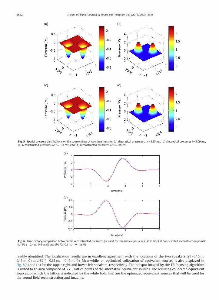
Fig. 5. Spatial pressure distributions on the source plane at two time instants: (a) theoretical pressures at t¼1.33 ms; (b) theoretical pressures t¼3.09 ms;(c) reconstructed pressures at t¼1.33 ms; and (d) reconstructed pressures at t¼3.09 ms.

0 1 2 3 4 5−4

−2

0

2

4

Time [ms]

Pre

ssur

e [P

a]

0 1 2 3 4 5−0.4

−0.2

0

0.2

0.4

Time [ms]

Pre

ssur

e [P

a]

Fig. 6. Time history comparison between the reconstructed pressures (þ) and the theoretical pressures (solid line) at two selected reconstruction points:(a) P1 (�0.4 m, 0.4 m, 0) and (b) P2 (0.1 m, �0.1 m, 0).

S. Pan, W. Jiang / Journal of Sound and Vibration 333 (2014) 3625–36383632

readily identified. The localization results are in excellent agreement with the locations of the two speakers, S1 (0.15 m,0.15 m, 0) and S2 (�0.15 m, �0.15 m, 0). Meanwhile, an optimized collocation of equivalent sources is also displayed inFig. 8(a) and (b) for the upper-right and lower-left speakers, respectively. The hotspot imaged by the TR focusing algorithmis suited to an area composed of 5�5 lattice points of the alternative equivalent sources. The resulting collocated equivalentsources, of which the lattice is indicated by the white bold line, are the optimized equivalent sources that will be used forthe sound field reconstruction and imaging.

Fig. 7. Experimental setups with two baffled loudspeakers, a triggering microphone and three types of microphone arrays: (a) TRM array; (b) patch array(the 5�5 microphones are only set in the white box); and (c) sparse array.

S. Pan, W. Jiang / Journal of Sound and Vibration 333 (2014) 3625–3638 3633

The second array was used in the hybrid reconstruction process and was named patch array, because it was configuredon the measurement and reconstruction planes, respectively, to face each patch of 5�5 optimized equivalent sourcesdetermined by the TRM procedure. The pressure field on the reconstruction plane, z¼0.02 m, was calculated by using theinterpolated TDESM. Two time instants, t¼1.17 ms and t¼2.15 ms, are chosen to display the out of phase spatial pressuredistributions measured on the reconstruction plane, as shown in Fig. 9(a) and (b), while the reconstructed pressures at thesetwo instants are presented in Fig. 9(c) and (d). According to Eq. (14), the calculated RMSEs of reconstruction at the two timeinstants are 21.00 and 19.10 percent, respectively. Fig. 10(a) and (b) shows the time history comparisons of reconstructedpressures with the measured pressures at two reconstruction points, P1 (0.05 m, 0.05 m, 0.02 m) and P2 (�0.25 m,�0.25 m, 0.02 m), respectively. Point P1 is located at the lower-left corner of the upper-right reconstructed area while pointP2 is located at the lower-left corner of the lower-left reconstructed area, and both points are on the up-to-right diagonal ofthe reconstruction plane. With the noise well suppressed, the agreement between the waveforms of reconstructed pressures

Table 1Parameters chosen for the TRM process of the numerical simulation and the experiment.

Case TRM array size Lattice spacing (m) Focusing plane size Lattice spacing (m) DMS (m) DFS (m)

Simulation 7�7 0.3 19�19 0.1 0.0134 0.0134Experiment 5�5 0.2 13�13 0.05 0.03 0.001

DMS stands for the distance between the measurement plane and the source plane.DFS stands for the distance between the focusing plane and the source plane.

Table 2Parameters chosen for the hybrid reconstruction process of the numerical simulation and the experiment.

Case Fundamental frequency (Hz) Patch array size Lattice spacing (m) DMS (m) DES (m) DRS (m)

Simulation 400 7�7 0.1 0.0134 0.0134 0Experiment 500 5�5 0.05 0.03 0.001 0.02

DES stands for the distance between the equivalent source plane and the source plane.DRS stands for the distance between the reconstruction plane and the source plane.

Fig. 8. Results of near-field TR source localization (relative value) and equivalent source collocation optimization for (a) the upper-right speaker and (b) thelower-left speaker at t¼2.7 ms.

S. Pan, W. Jiang / Journal of Sound and Vibration 333 (2014) 3625–36383634

and those of measured pressures is very satisfactory for the experimental condition. The calculated RMSEs at these twopoints are 4.56 and 5.81 percent, respectively.

The third array, which had sparser microphone spacing than the patch array, was named sparse array and utilized tocarry out the transient sound field reconstruction by using the original interpolated TDESM directly. The position of theequivalent source, measurement and reconstruction planes remained the same as in the hybrid procedure. The distributions

Fig. 9. Spatial pressure distributions on the reconstruction plane at two time instants: (a) measured pressures at t¼1.17 ms; (b) measured pressurest¼2.15 ms; (c) reconstructed pressures at t¼1.17 ms; and (d) reconstructed pressures at t¼2.15 ms.

0 1 2 3 4 5−0.15

−0.1

−0.05

0

0.05

0.1

Time [ms]

Pre

ssur

e [P

a]

0 1 2 3 4 5−0.1

−0.05

0

0.05

0.1

0.15

Time [ms]

Pre

ssur

e [P

a]

Fig. 10. Time history comparison between the reconstructed pressures (þ) and the measured pressures (solid line) at two selected reconstruction points:(a) P1 (0.05 m, 0.05 m, 0.02 m) and (b) P2 (�0.25 m, �0.25 m, 0.02 m).

S. Pan, W. Jiang / Journal of Sound and Vibration 333 (2014) 3625–3638 3635

of equivalent sources and reconstruction points in x and y directions are the same as the microphones of the sparse array(7�7 array with equal lattice spacing 0.1 m).

For the same reason as the hybrid procedure, two time instants, t¼1.95 ms and t¼2.34 ms, are selected to display the outof phase spatial pressure distributions measured on the reconstruction plane. Fig. 11(a) and (b) shows the measuredpressures at these two instants, while the reconstructed pressures are presented in Fig. 11(c) and (d). It can be seen that theresolution of images in Fig. 11 is much lower than that when using the hybrid technique (see Fig. 9). The calculated RMSEs atthese two time instants are 22.33 and 26.30 percent, respectively. In contrast to the imaging results obtained by the hybrid

Fig. 11. Spatial pressure distributions on the reconstruction plane at two time instants: (a) measured pressures at t¼1.95 ms; (b) measured pressurest¼2.34 ms; (c) reconstructed pressures at t¼1.95 ms; and (d) reconstructed pressures at t¼2.34 ms.

0 1 2 3 4 5−0.2

−0.1

0

0.1

0.2

Time [ms]

Pre

ssur

e [P

a]

0 1 2 3 4 5−0.1

−0.05

0

0.05

0.1

Time [ms]

Pre

ssur

e [P

a]

Fig. 12. Time history comparison between the reconstructed pressures (þ) and the measured pressures (solid line) at two selected reconstruction points:(a) P1 (0.3 m, 0.3 m, 0.02 m) and (b) P2 (0, 0, 0.02 m).

S. Pan, W. Jiang / Journal of Sound and Vibration 333 (2014) 3625–36383636

technique, the spatial distribution features of the transient sound field are unable to be accurately visualized. Fig. 12(a) and (b)shows the time history comparisons of reconstructed pressures and the measured pressures at two reconstruction points, P1(0.3 m, 0.3 m, 0.02 m) and P2 (0, 0, 0.02 m), respectively. Points P1 and P2 are located at the upper-right corner and the center ofthe entire reconstructed area, respectively, and both points are on the up-to-right diagonal of the reconstruction plane. Even ifthe noise is well suppressed, the amplitudes of reconstructed pressures are lower than those of measured pressures at most ofthe reconstructed time instants. The calculated RMSEs at the two points are 17.08 and 22.87 percent, respectively.

0 1 2 3 4 50

0.1

0.2

0.3

0.4

0.5

0.6

0.7

0.8

Time [ms]

RM

SE

HybridOriginal

Fig. 13. Experimental RMSE–time curves calculated by using the hybrid technique and the original interpolated TDESM, respectively.

S. Pan, W. Jiang / Journal of Sound and Vibration 333 (2014) 3625–3638 3637

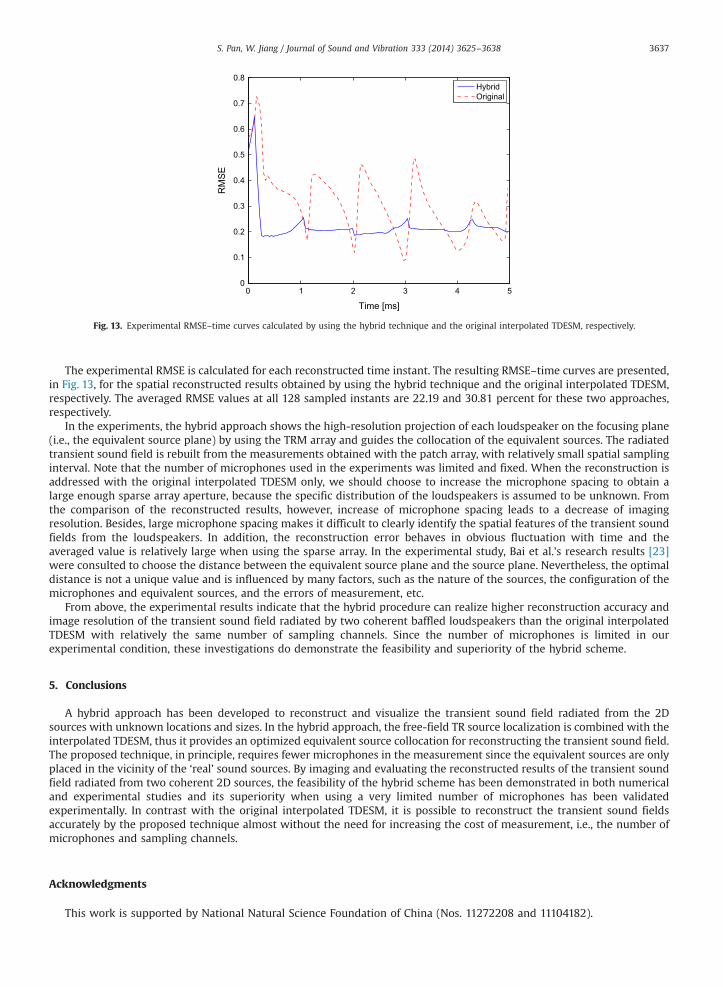
The experimental RMSE is calculated for each reconstructed time instant. The resulting RMSE–time curves are presented,in Fig. 13, for the spatial reconstructed results obtained by using the hybrid technique and the original interpolated TDESM,respectively. The averaged RMSE values at all 128 sampled instants are 22.19 and 30.81 percent for these two approaches,respectively.

In the experiments, the hybrid approach shows the high-resolution projection of each loudspeaker on the focusing plane(i.e., the equivalent source plane) by using the TRM array and guides the collocation of the equivalent sources. The radiatedtransient sound field is rebuilt from the measurements obtained with the patch array, with relatively small spatial samplinginterval. Note that the number of microphones used in the experiments was limited and fixed. When the reconstruction isaddressed with the original interpolated TDESM only, we should choose to increase the microphone spacing to obtain alarge enough sparse array aperture, because the specific distribution of the loudspeakers is assumed to be unknown. Fromthe comparison of the reconstructed results, however, increase of microphone spacing leads to a decrease of imagingresolution. Besides, large microphone spacing makes it difficult to clearly identify the spatial features of the transient soundfields from the loudspeakers. In addition, the reconstruction error behaves in obvious fluctuation with time and theaveraged value is relatively large when using the sparse array. In the experimental study, Bai et al.'s research results [23]were consulted to choose the distance between the equivalent source plane and the source plane. Nevertheless, the optimaldistance is not a unique value and is influenced by many factors, such as the nature of the sources, the configuration of themicrophones and equivalent sources, and the errors of measurement, etc.

From above, the experimental results indicate that the hybrid procedure can realize higher reconstruction accuracy andimage resolution of the transient sound field radiated by two coherent baffled loudspeakers than the original interpolatedTDESM with relatively the same number of sampling channels. Since the number of microphones is limited in ourexperimental condition, these investigations do demonstrate the feasibility and superiority of the hybrid scheme.

5. Conclusions

A hybrid approach has been developed to reconstruct and visualize the transient sound field radiated from the 2Dsources with unknown locations and sizes. In the hybrid approach, the free-field TR source localization is combined with theinterpolated TDESM, thus it provides an optimized equivalent source collocation for reconstructing the transient sound field.The proposed technique, in principle, requires fewer microphones in the measurement since the equivalent sources are onlyplaced in the vicinity of the ‘real’ sound sources. By imaging and evaluating the reconstructed results of the transient soundfield radiated from two coherent 2D sources, the feasibility of the hybrid scheme has been demonstrated in both numericaland experimental studies and its superiority when using a very limited number of microphones has been validatedexperimentally. In contrast with the original interpolated TDESM, it is possible to reconstruct the transient sound fieldsaccurately by the proposed technique almost without the need for increasing the cost of measurement, i.e., the number ofmicrophones and sampling channels.

Acknowledgments

This work is supported by National Natural Science Foundation of China (Nos. 11272208 and 11104182).

S. Pan, W. Jiang / Journal of Sound and Vibration 333 (2014) 3625–36383638

References

[1] J.D. Maynard, E.G. Williams, Y. Lee, Nearfield acoustic holography: I. Theory of generalized holography and the development of NAH, The Journal of theAcoustical Society of America 78 (1985) 1395–1413.

[2] W.A. Veronesi, J.D. Maynard, Nearfield acoustic holography (NAH) II. Holographic reconstruction algorithms and computer implementation, TheJournal of the Acoustical Society of America 81 (1987) 1307–1322.

[3] E.G. Williams, J.D. Maynard, Holographic imaging without the wavelength resolution limit, Physical Review Letters 45 (1980) 554–557.[4] J.H. Thomas, V. Grulier, S. Paillasseur, J.C. Pascal, J.C. Le Roux, Real-time near-field acoustic holography for continuously visualizing nonstationary

acoustic fields, Journal of the Acoustical Society of America 128 (2010) 3554–3567.[5] J.F. Blais, A. Ross, Forward projection of transient sound pressure fields radiated by impacted plates using numerical Laplace transform, Journal of the

Acoustical Society of America 125 (2009) 3120–3128.[6] X.Z. Zhang, J.H. Thomas, C.X. Bi, J.C. Pascal, Reconstruction of nonstationary sound fields based on the time domain plane wave superposition method,

Journal of the Acoustical Society of America 132 (2012) 2427–2436.[7] S.F. Wu, H. Lu, M.S. Bajwa, Reconstruction of transient acoustic radiation from a sphere, Journal of the Acoustical Society of America 117 (2005)

2065–2077.[8] M.R. Bai, J.-H. Lin, Source identification system based on the time-domain nearfield equivalence source imaging: fundamental theory and

implementation, Journal of Sound and Vibration 307 (2007) 202–225.[9] M.R. Bai, J.-H. Lin, C.-W. Tseng, Implementation issues of the nearfield equivalent source imaging microphone array, Journal of Sound and Vibration 330

(2011) 545–558.[10] S. Lee, Prediction of Acoustic Scattering in the Time Domain and its Applications to Rotorcraft Noise, PhD Thesis, Pennsylvania State University, 2009.[11] S. Lee, K.S. Brentner, P.J. Morris, Acoustic scattering in the time domain using an equivalent source method, AIAA Journal 48 (2010) 2772–2780.[12] S. Lee, K.S. Brentner, P.J. Morris, Assessment of time-domain equivalent source method for acoustic scattering, AIAA Journal 49 (2011) 1897–1906.[13] X.Z. Zhang, C.X. Bi, Y.B. Zhang, L. Xu, Transient nearfield acoustic holography based on an interpolated time-domain equivalent source method, Journal

of the Acoustical Society of America 130 (2011) 1430–1440.[14] C.X. Bi, L. Geng, X.Z. Zhang, Cubic spline interpolation-based time-domain equivalent source method for modeling transient acoustic radiation, Journal

of Sound and Vibration 332 (2013) 5939–5952.[15] J. Hald, Combined NAH and beamforming using the same microphone array, Sound and Vibration 38 (2004) 18–27.[16] S. Gade, J. Hald, B. Ginn, Refined beamforming with increased spatial resolution, Proceedings of the INTER-NOISE and NOISE-CON Congress and

Conference, Institute of Noise Control Engineering, New York, USA, 2012, pp. 9228–9235.[17] M. Fink, Time reversal of ultrasonic fields. I. Basic principles, IEEE Transactions on Ultrasonics, Ferroelectrics and Frequency Control 39 (1992) 555–566.[18] E. Bavu, C. Besnainou, V. Gibiat, J. De Rosny, M. Fink, Subwavelength sound focusing using a time-reversal acoustic sink, Acta Acustica United with

Acustica 93 (2007) 706–715.[19] E. Bavu, A. Berry, High-resolution imaging of sound sources in free field using a numerical time-reversal sink, Acta Acustica United with Acustica 95

(2009) 595–606.[20] S. Pan, W. Jiang, Optimized two-dimensional imaging of transient sound fields using a hybrid transient acoustic holography, Proceedings of Meetings on

Acoustics 19 (2013) 055012.[21] E.G. Williams, Regularization methods for near-field acoustical holography, The Journal of the Acoustical Society of America 110 (2001) 1976–1988.[22] S.-H. Yoon, P.A. Nelson, Estimation of acoustic source strength by inverse methods: Part II, experimental investigation of methods for choosing

regularization parameters, Journal of Sound and Vibration 233 (2000) 665–701.[23] M.R. Bai, C.C. Chen, J.H. Lin, On optimal retreat distance for the equivalent source method-based nearfield acoustical holography, Journal of the

Acoustical Society of America 129 (2011) 1407–1416.