Analytical integrations of the linearly interpolated ... integrations of the linearly interpolated triangular IBEM element ... in an indirect boundary element method ... Matlab codes

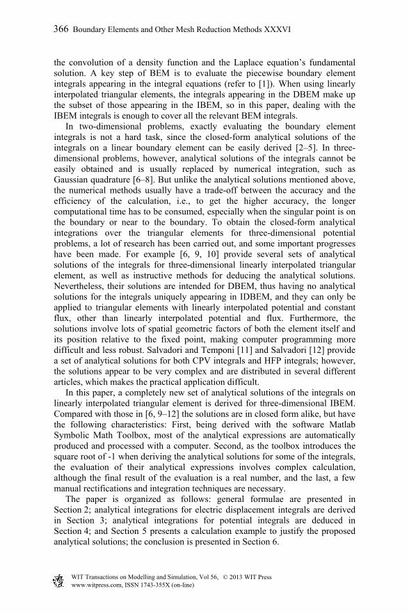
Analytical integrations of the linearly interpolated triangular IBEM element with the aid of the Matlab Symbolic Math Toolbox

Gong Andong School of Geosciences and Info-physics, Central South University, P. R. China

Abstract

This paper deals with the analytical integration over the linearly interpolated triangular boundary element involved in an indirect boundary element method (IBEM) for solving three dimensional potential problems. The analytical solutions of all the IBEM integrals are derived using the Matlab Symbolic Math Toolbox, with most of the deriving works carried out by computer, and accompanied by a few crucial manual rectifications and integrating techniques. Compared with the presently published kindred analytical solutions, the computer-produced and human-rectified ones take much less tedious manual work and have their own advantages in implementation, such as convenience for programming, and no need to trace the relevant literature for detailed expressions, etc. A calculation test is also carried out to justify the analytical solutions. Keywords: indirect boundary element method, triangular element, analytical integration, Matlab Symbolic Math Toolbox.

1 Introduction

The boundary element method (BEM) plays an important role in the solution of the potential problems which are governed by the Laplace equation or Poisson equation owing to its much lower requirement for computer memory and obvious superiority in solving infinite-boundary problems. Depending on the boundary integral equations (BIE) applied, BEM can be divided into direct boundary element method (DBEM) and indirect boundary element method (IBEM). The former uses the second Green formula as BIE, while the latter uses

Boundary Elements and Other Mesh Reduction Methods XXXVI 365

www.witpress.com, ISSN 1743-355X (on-line) WIT Transactions on Modelling and Simulation, Vol 56, © 2013 WIT Press

doi:10.2495/BEM360301

the convolution of a density function and the Laplace equation’s fundamental solution. A key step of BEM is to evaluate the piecewise boundary element integrals appearing in the integral equations (refer to [1]). When using linearly interpolated triangular elements, the integrals appearing in the DBEM make up the subset of those appearing in the IBEM, so in this paper, dealing with the IBEM integrals is enough to cover all the relevant BEM integrals. In two-dimensional problems, exactly evaluating the boundary element integrals is not a hard task, since the closed-form analytical solutions of the integrals on a linear boundary element can be easily derived [2–5]. In three-dimensional problems, however, analytical solutions of the integrals cannot be easily obtained and is usually replaced by numerical integration, such as Gaussian quadrature [6–8]. But unlike the analytical solutions mentioned above, the numerical methods usually have a trade-off between the accuracy and the efficiency of the calculation, i.e., to get the higher accuracy, the longer computational time has to be consumed, especially when the singular point is on the boundary or near to the boundary. To obtain the closed-form analytical integrations over the triangular elements for three-dimensional potential problems, a lot of research has been carried out, and some important progresses have been made. For example [6, 9, 10] provide several sets of analytical solutions of the integrals for three-dimensional linearly interpolated triangular element, as well as instructive methods for deducing the analytical solutions. Nevertheless, their solutions are intended for DBEM, thus having no analytical solutions for the integrals uniquely appearing in IDBEM, and they can only be applied to triangular elements with linearly interpolated potential and constant flux, other than linearly interpolated potential and flux. Furthermore, the solutions involve lots of spatial geometric factors of both the element itself and its position relative to the fixed point, making computer programming more difficult and less robust. Salvadori and Temponi [11] and Salvadori [12] provide a set of analytical solutions for both CPV integrals and HFP integrals; however, the solutions appear to be very complex and are distributed in several different articles, which makes the practical application difficult. In this paper, a completely new set of analytical solutions of the integrals on linearly interpolated triangular element is derived for three-dimensional IBEM. Compared with those in [6, 9–12] the solutions are in closed form alike, but have the following characteristics: First, being derived with the software Matlab Symbolic Math Toolbox, most of the analytical expressions are automatically produced and processed with a computer. Second, as the toolbox introduces the square root of -1 when deriving the analytical solutions for some of the integrals, the evaluation of their analytical expressions involves complex calculation, although the final result of the evaluation is a real number, and the last, a few manual rectifications and integration techniques are necessary. The paper is organized as follows: general formulae are presented in Section 2; analytical integrations for electric displacement integrals are derived in Section 3; analytical integrations for potential integrals are deduced in Section 4; and Section 5 presents a calculation example to justify the proposed analytical solutions; the conclusion is presented in Section 6.

366 Boundary Elements and Other Mesh Reduction Methods XXXVI


2 General formulae

Potential problems include electrostatic, gravitational, and steady-state heat conducting problems, etc. Without loss of generality, we take the electrostatic problem as example in this paper. In a typical three-dimensional electrostatic problem, the Laplace equation can be written as

2 ( , , ) 0u x y z , (1)

which governs the potential u in a three-dimensional domain enclosed by a boundary surface . Suppose that is enclosed by a virtual boundary surface , and there is an interval between the two surfaces. is divided into a certain number of triangular elements, with neighboring elements having two common vertexes, the standard IBEM procedure leads to the following equation:

1

31

1 1

4

1

4

e

n

e

n

N

jn

N

jn

u q dr

rD q d

r

(2)

where Ne is the total number of the elements on , n denotes the integration area of the nth element, uj denotes the potential value at collocation point Pj, jD

denotes the electric displacement vector at Pj, q denotes the linearly

interpolated density of the source charge on the element, and r

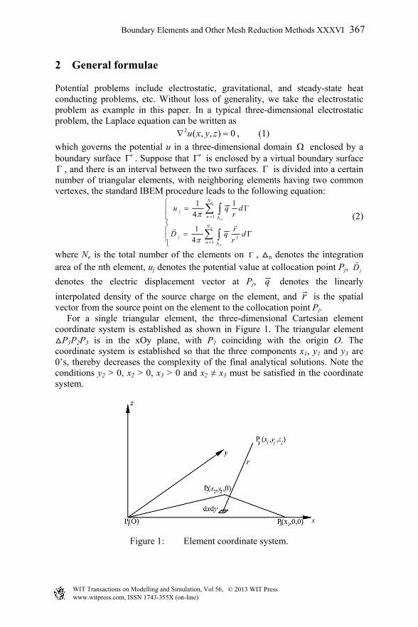
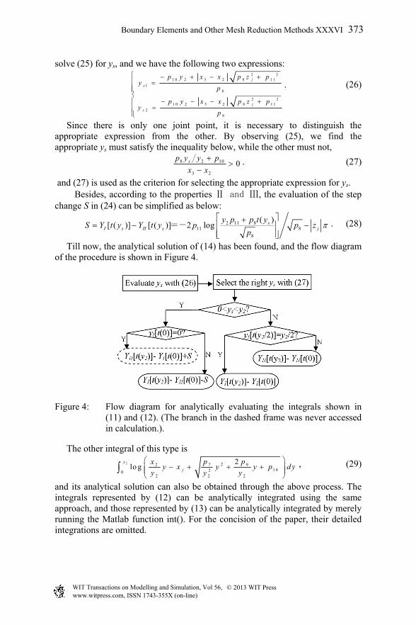
is the spatial vector from the source point on the element to the collocation point Pj. For a single triangular element, the three-dimensional Cartesian element coordinate system is established as shown in Figure 1. The triangular element

P1P2P3 is in the xOy plane, with P1 coinciding with the origin O. The coordinate system is established so that the three components x1, y1 and y3 are 0’s, thereby decreases the complexity of the final analytical solutions. Note the conditions y2 > 0, x2 > 0, x3 > 0 and x2 ≠ x3 must be satisfied in the coordinate system.

Figure 1: Element coordinate system.



In the triangular element shown in Figure 1, the source charge density q are

linearly interpolated as below:

1 1 2 2 3 3( , )q x y N q N q N q , (3)

where

2 31

3 2 3

( )1

x x yxN

x y x

, 2

2

yN

y , 2

33 2 3

x yxN

x y x ,

are the linear shape functions. Substitute (3) into (2), and after algebraic manipulations, we have

1

31

31

31

1 1( )

4

1( )

4

1( )

4

1( )

4

e

n

e

n

e

n

e

n

Nq q q

j n n nn

Njq q q

jx n n nn

Njq q q

jy n n nn

Njq q q

jz n n nn

u a b x c y dxdyr

x xD a b x c y dxdy

r

y yD a b x c y dxdy

r

zD a b x c y dxdy

r

, (4)

where 2 2 2( ) ( )j j jr x x y y z , denoting the distance between (x, y) on

the element and Pj (xj, yj, zj) (see Figure 1), Djx, Djy, and Djz are the three components of the electric displacement movement vector. For an element, the expressions of the coefficients aq, bq, and cq are as follows:

1qa q ; 3 1

3

q q qb

x

; 2 3 1 3 2 2 3

3 2

q x x q x q x qc

x y

.

To proceed with the IBEM, the next step is to calculate the following integrals which are extracted from (4):

2 3

322

2

2

( )

0 2 2 2( ) ( )

x x yxy yx yk

y j j j

AG dxdy

x x y y z

(5)

2 3

322

2

2

( )

1 .50 2 2 2( ) ( )

x x yxy yx yl

y j j j

A BH dxdy

x x y y z

(6)

where A∈｛1,x,y｝，B∈｛xj -x, yj -y , zj ｝，k =1 to 3, and l = 1 to 9. So (5) and (6) represent twelve integrals altogether. The three integrals represented by (5) are named potential integrals and the three integrals represented by (6) are named electric displacement integrals in this paper, since they are used to calculate the potential and the electric displacement at Pj respectively.

3 Analytical integrations for the electric displacement integrals

Using the Symbolic Math Toolbox of Matlab, the analytical solutions for the integrals in (6) can be obtained in the form of symbolic strings. Here we take the integral



2 332

2

2

2

( )

1.50 2 2 2( ) ( )

x x yxy yx y

y j j j

yH dxdy

x x y y z

as a representative example to demonstrate the detailed integration method. First, run the following Matlab codes in the Matlab command window, where the italic text following the symbol ‘%’ is the comment for the code in the next line.

%Prepare the string representing the integrand. s='y/((yj-y)^2+(xj-x)^2+zj^2)^1.5'; %Integrate with respect to ‘x’ r1=int(s, 'x', 'x2*y/y2','x3+(x2-x3)*y/y2'); %Integrate with respect to ‘y’ r2=int(r1,'y','0','y2'); %Substitute the imaginary unit i for the square root of -1. r2=subs(r2,'(-1.*zj^2)^(1/2)','(i*zj)');

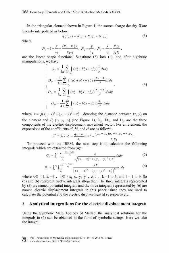
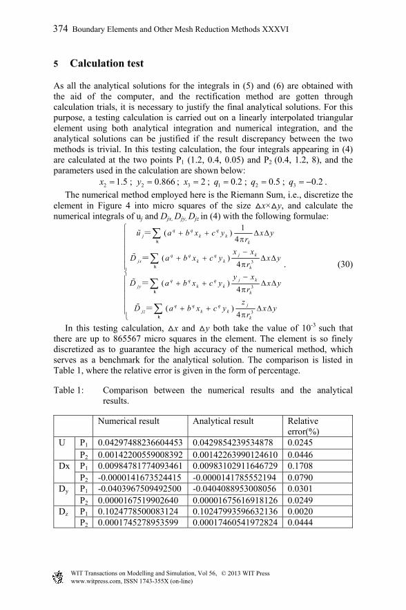
after the codes are executed, the computer-produced and closed-form analytical solution can be found in the string-type variable r2. Using a few string processing functions in the Matlab symbolic toolbox, it can be simplified to a much shorter string. However, if we evaluate the solution now, we will find that it may produce distorted result. Figure 2 is the continuously evaluated result of r2 illustrated using the Matlab plot function, with xj = 0 to 3, yj = 0.4, zj = 0.21, x2 = 2.5, y2 = 0.866, x3 = 4. From Figure 2(a) which illustrates the directly evaluated r2, it can be seen that the plotted curve is not continuous, and there are two step-changes near the points xj = 0.75 and xj = 1.5 respectively, which distort the evaluation.

(a) (b)

Figure 2: The evaluated result of the analytical solution before and after rectification.

After a lot of calculation trials, we find that the distortion is caused by the atanh() function in the r2, for the reason that every time a step-change happens during the process of the continuous evaluation, a sign shift between ‘+’ and ‘-’ occurs on the imaginary part of the atanh() function’s output value. Therefore,



one of the approach to avoid the distortion is to keep the imaginary part positive using the following procedure:

atanh(b)→a; if imag(a) < 0 then (a + i) →a; where the variables a and b are of complex type, representing the output and input values of the atanh() function, and the function imag() takes the imaginary part of a. After the rectification, the final expression of the analytical solution is given below:

3 2 223 24 22 20 21 19

8 7

real ij j

x x xH y z p p p p p p

p p

, (7)

where the function real() takes the real part of the input complex value, and the analytical expressions of pn in (7) and other parts of the paper are listed in Appendix A. The analytical solutions for the other 8 electric displacement integrals have also been derived using the Matlab Symbolic Math Toolbox, and their deriving method and rectification method are generally the same as the above, for the sake of concision, they are not listed in this paper.

4 Analytical integrations for the potential integrals

Unlike the integrals in (6), the analytical solutions of those in (5) cannot be obtained by calling the int() function twice. To get their analytical solution using Matlab, some integration techniques must be used manually.

4.1 Inner integrations for 1G , 2G and 3G

For the three integrals in (5), first perform the inner integrations with respect to x using the Matlab’s int() function, and we have:

2

2

22 3 8 101 3 1320

2 22

27 921420

2 22

2log

2log

y

j

y

j

x x p pG y x x y y p dy

y yy

p pxy x y y p dy

y yy

＋, (8)

2 2 28 10 7 92 1 13 142 20

2 22 2

2 2y

j

p p p pG x G y y p y y p dy

y yy y

+ - , (9)

2

2

22 3 8 103 3 1320

2 22

27 921420

2 22

2log

2log

y

j

y

j

x x p pG y x x y y p ydy

y yy

p pxy x y y p ydy

y yy

＋

(10)

From (8) to (10), it can be seen that G1, G2 and G3 are linear combinations of the following three types of integrals:

2 2

0log

yay b cy dy e dy , (11)



2 2

0log

yay b cy dy e ydy , (12)

2 2 2

0

ycy dy e c y d y e dy ‘ ’ ‘－ , (13)

where the a, b, c, d, e and c’, d’, e’ represent the constant real coefficients shown in (8) and (9), and these coefficients depend on the coordinates of the element vertexes and the point Pj (see Figure 1). So, it is essential to find the analytical solutions of the three types of integrals.

4.2 Analytical solutions of the integrals represented by (11)

One of the integrals represented by (11) is

2 22 3 8 103 1320

2 22

2log

y

j

x x p py x x y y p dy

y yy

＋ . (14)

Let

22 3 8 103 132

2 22

2( ) j

x x p pt y y x x y y p

y yy

＋ , (15)

substitute it into (14), and perform integration by part, then we have:

2

2

( )

0(0 )

( )log( ) ( ) log( )

t yy

t

y tt dy y t t dt

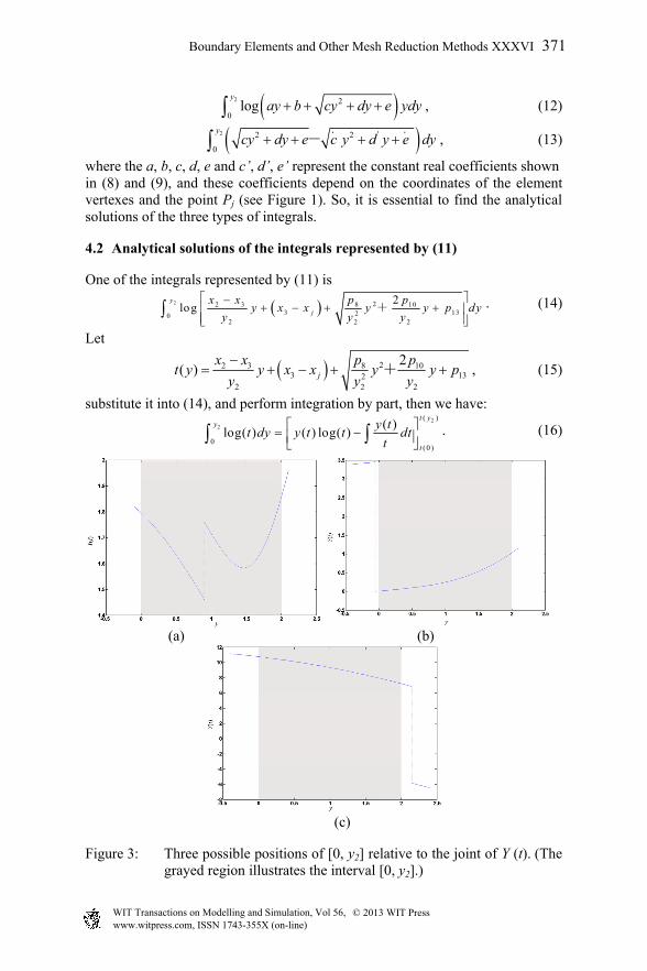
t . (16)

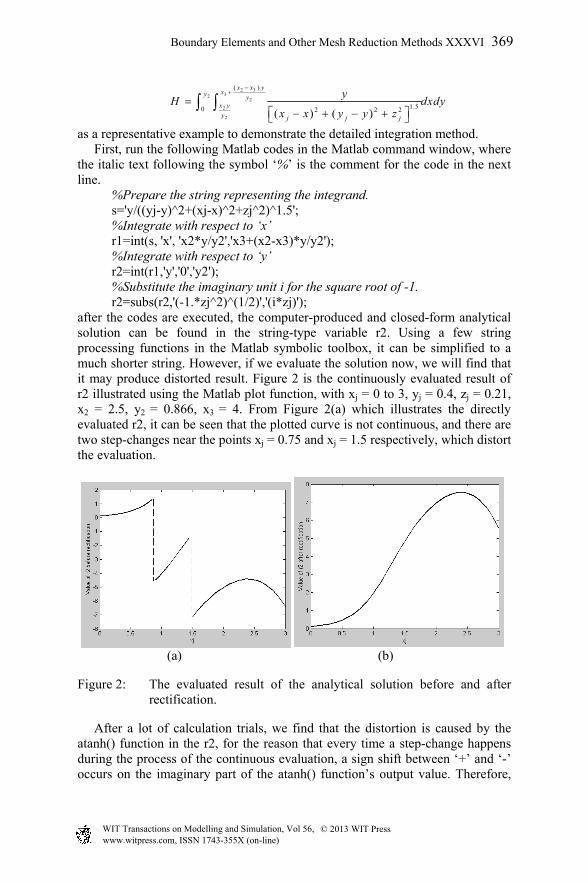
(a) (b)

(c)

Figure 3: Three possible positions of [0, y2] relative to the joint of Y (t). (The grayed region illustrates the interval [0, y2].)



where the part in the square bracket is denoted with Y (t), i.e.,

( )( ) ( ) log( )

y tY t y t t dt

t ＝ . (17)

Solve the equation of (15) for y, and the following two expressions are obtained:

2 2 28 2 1 1 23 2

2 2

2 2 28 2 1 1 23 2

2 2

2( )

2( )

j

I j

j

I I j

p t y p t z yx xy t y t

y y

p t y p t z yx xy t y t

y y

(18)

Substitute them into (17) separately and solve the indefinite integrals, then we have two analytical expressions for Y (t), which are shown below:

2

11 226 11

8 25

( ) ( ) log( ) 1 atan jI I j j

j

p t z yp pY t y t y t z

p z p

＝ , (19)

2

11 226 11

8 25

( ) ( ) log( ) 1 atan j

j jII II

j

p t z yp pY t y t y t z

p z p

＝ . (20)

Since t is a function of y, Y (t) is also a function of y, and it is expressed with YI (t) and YII (t) conditionally and sectionally, i.e., for an arbitrary y,

( ) if ( )( )

( ) if ( )I I

II II

Y t y y t yY t

Y t y y t y

. (21)

The graph of Y (t) vs. y can be plotted in accordance with (21), and the plotted curve is generally continuous and smooth, except for a step change at the joint of YI (t) and YII (t).Thus, to evaluate the 2( )

(0)( )

t y

tY t in (16), three possible positions of

the interval [0, y2] relative to the joint point ys have to be considered (see Figure 3 where all curves are plotted with y2 = 2): If the interval [0, y2] is covered by YI (t) as shown in Figure 3(a),

2 2( )

2(0)0log( ) ( ) ( ) (0)

y t y

I Itt dy Y t Y t y Y t ; (22)

if [0, y2] is covered by YII (t) as shown in Figure 3(b),

2 2( )

2(0)0log( ) ( ) ( ) (0)

y t y

II IItt dy Y t Y t y Y t ; (23)

in the case that the joint point ys is within [0, y2], as shown in Figure 3(c), the step change has to be eliminated, and we have

2 2( )

2( 0 )0log( ) ( ) ( ) (0)

y t y

tt dy Y t Y t y Y t S , (24)

where S = YI [t(ys)] – YII [t(ys)], denoting the step change at ys. Now the problem is how to evaluate the ys which denotes the position of the joint point. It can be proved that the ys has the following three properties:

�. ( )0

sy y

dt y

dy ;Ⅱ. ( ) ( )I s II sy t y y t y＝ ; Ⅲ. 2 2 28 2 11 2( ) 2 ( ) 0s s jp t y y p t y z y .

From the propertyⅠ, we know the ys must satisfy the following equality:

2 2 8 2 108 2 10 2 13

3 2

2 ss s

p y y pp y y p y y p

x x

, (25)



solve (25) for ys, and we have the following two expressions:

2 2

1 0 2 3 2 8 1 1

18

2 21 0 2 3 2 8 1 1

28

j

s

j

s

p y x x p z py

p

p y x x p z py

p

. (26)

Since there is only one joint point, it is necessary to distinguish the appropriate expression from the other. By observing (25), we find the appropriate ys must satisfy the inequality below, while the other must not,

8 2 10

3 2

0sp y y p

x x

. (27)

and (27) is used as the criterion for selecting the appropriate expression for ys. Besides, according to the properties Ⅱ and Ⅲ, the evaluation of the step

change S in (24) can be simplified as below:

2 11 811 8

8

( )[ ( )] [ ( )] 2 log s

s s j

y p p t yS Y t y Y t y p p z

p

＝－ . (28)

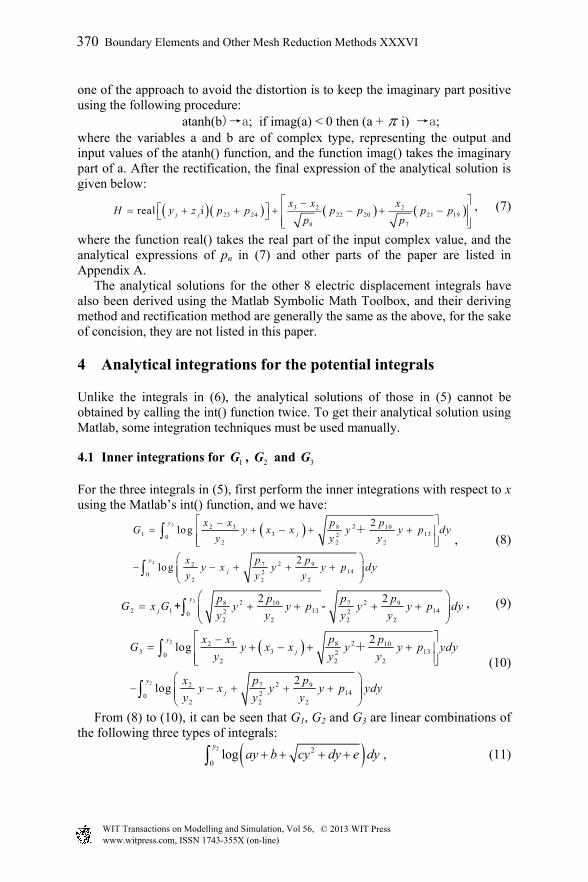
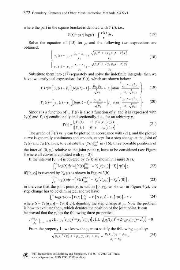
Till now, the analytical solution of (14) has been found, and the flow diagram of the procedure is shown in Figure 4.

Figure 4: Flow diagram for analytically evaluating the integrals shown in (11) and (12). (The branch in the dashed frame was never accessed in calculation.).

The other integral of this type is

2 27 921 420

2 22

2lo g

y

j

p pxy x y y p d y

y yy

, (29)

and its analytical solution can also be obtained through the above process. The integrals represented by (12) can be analytically integrated using the same approach, and those represented by (13) can be analytically integrated by merely running the Matlab function int(). For the concision of the paper, their detailed integrations are omitted.



5 Calculation test

As all the analytical solutions for the integrals in (5) and (6) are obtained with the aid of the computer, and the rectification method are gotten through calculation trials, it is necessary to justify the final analytical solutions. For this purpose, a testing calculation is carried out on a linearly interpolated triangular element using both analytical integration and numerical integration, and the analytical solutions can be justified if the result discrepancy between the two methods is trivial. In this testing calculation, the four integrals appearing in (4) are calculated at the two points P1 (1.2, 0.4, 0.05) and P2 (0.4, 1.2, 8), and the parameters used in the calculation are shown below:

2 1.5x ; 2 0.866y ; 3 2x ; 1 0.2q ; 2 0.5q ; 3 0.2q .

The numerical method employed here is the Riemann Sum, i.e., discretize the element in Figure 4 into micro squares of the size x× y, and calculate the numerical integrals of uj and Djx, Djy, Djz in (4) with the following formulae:

3

3

3

1( )

4

( )4

( )4

( )4

q q qj k k

k

j kq q qjx k k

k

j kq q qjy k k

k

jq q qjz k k

k

u a b x c y x yr

x xD a b x c y x y

r

y xD a b x c y x y

r

zD a b x c y x y

r

k

k

k

k

＝

＝

＝

＝

. (30)

In this testing calculation, x and y both take the value of 10-3 such that there are up to 865567 micro squares in the element. The element is so finely discretized as to guarantee the high accuracy of the numerical method, which serves as a benchmark for the analytical solution. The comparison is listed in Table 1, where the relative error is given in the form of percentage.

Table 1: Comparison between the numerical results and the analytical results.

Numerical result Analytical result Relative error(%)

U P1 0.04297488236604453 0.0429854239534878 0.0245 P2 0.00142200559008392 0.00142263990124610 0.0446

Dx P1 0.00984781774093461 0.00983102911646729 0.1708 P2 -0.0000141673524415 -0.0000141785552194 0.0790

Dy P1 -0.0403967509492500 -0.0404088953008056 0.0301 P2 0.0000167519902640 0.00001675616918126 0.0249

Dz P1 0.1024778500083124 0.10247993596632136 0.0020 P2 0.0001745278953599 0.00017460541972824 0.0444



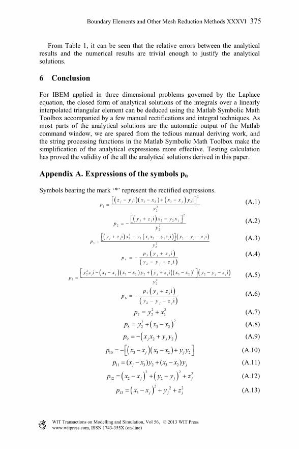
From Table 1, it can be seen that the relative errors between the analytical results and the numerical results are trivial enough to justify the analytical solutions.

6 Conclusion

For IBEM applied in three dimensional problems governed by the Laplace equation, the closed form of analytical solutions of the integrals over a linearly interpolated triangular element can be deduced using the Matlab Symbolic Math Toolbox accompanied by a few manual rectifications and integral techniques. As most parts of the analytical solutions are the automatic output of the Matlab command window, we are spared from the tedious manual deriving work, and the string processing functions in the Matlab Symbolic Math Toolbox make the simplification of the analytical expressions more effective. Testing calculation has proved the validity of the all the analytical solutions derived in this paper.

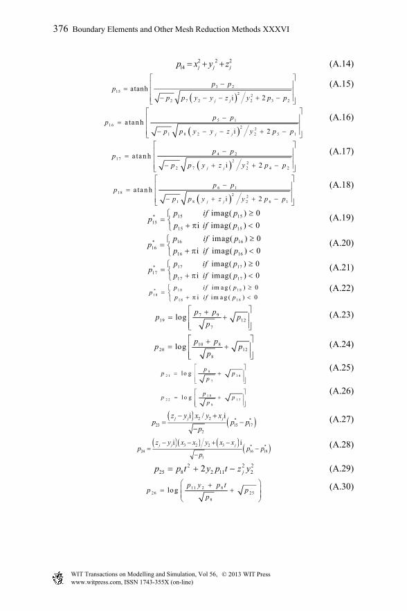
Appendix A. Expressions of the symbols pn

Symbols bearing the mark ‘*’ represent the rectified expressions.

2

3 2 3 2

1 22

i ij j jz y x x x x yp

y

(A.1)

2

2 2

2 22

ij j jy z x y xp

y

(A.2)

22 2 2 2 2

3 22

i i ij j j j j jy z x y x x y z y y zp

y

(A.3)

3

4

2

i

i

j j

j j

p y zp

y y z

(A.4)

222 3 3 2 2 3 2 2

5 22

i i ij j j j j jy z x x x x y y z x x y y zp

y

(A.5)

5

6

2

i

i

j j

j j

p y zp

y y z

(A.6)

2 27 2 2p y x (A.7)

228 2 3 2p y x x (A.8)

9 2 2j jp x x y y (A.9)

10 3 3 2 2j jp x x x x y y (A.10)

11 3 2 3 2( ) ( )j jp x x y x x y (A.11)

2 2 212 2 2j j jp x x y y z (A.12)

2 2 213 3 j j jp x x y z (A.13)



2 2 214 j j jp x y z (A.14)

3 2

15 2 22 7 2 2 3 2

atanhi 2j j

p pp

p p y y z y p p

(A.15)

5 1

1 6 2 21 8 2 2 5 1

a tan hi 2j j

p pp

p p y y z y p p

(A.16)

4 2

1 7 2 22 7 2 4 2

a tan hi 2j j

p pp

p p y z y p p

(A.17)

6 1

1 8 2 21 8 2 6 1

a tan hi 2j j

p pp

p p y z y p p

(A.18)

15 15*15

15 15

imag( ) 0

i imag( ) 0

p if pp

p if p

(A.19)

16 16*16

16 16

imag( ) 0

i imag( ) 0

p if pp

p if p

(A.20)

17 17*17

17 17

imag( ) 0

i imag( ) 0

p if pp

p if p

(A.21)

1 8 1 8*1 8

1 8 1 8

im a g ( ) 0

i im a g ( ) 0

p i f pp

p if p

(A.22)

7 919 12

7

logp p

p pp

(A.23)

10 820 12

8

logp p

p pp

(A.24)

9

2 1 1 4

7

lo gp

p pp

(A.25)

1 0

2 2 1 3

8

l o gp

p pp

(A.26)

2 2 * *23 15 17

2

i / ij j jz y x y xp p p

p

(A.27)

3 2 2 3 * *24 16 18

1

i ij j jz y x x y x xp p p

p

(A.28)

2 2 225 8 2 11 22 jp p t y p t z y (A.29)

11 2 826 25

8

logp y p t

p pp

(A.30)



References

[1] P. A. Martin, F. J. Rizzo, Hypersingular integrals: how smooth must the density be? International Journal for Numerical Methods in Engineering. 39 (1996) 687-704.

[2] Friedrich J, A linear analytical boundary element method (BEM) for 2D homogeneous potential problems, Computers & Geosciences. 28 (2002) 679-692.

[3] Huanlin Zhou, Zhongrong Niu, Changzheng Cheng, Zhongwei Guan, Analytical integral algorithm applied to boundary layer effect and thin body effect in BEM for anisotropic potential problems, Computers and Structures. 86 (2008) 1656-1671.

[4] Huanlin Zhou, Zhongrong Niu, Changzheng Cheng, Zhongwei Guan, Analytical integral algorithm in the BEM for orthotropic potential problems of thin bodies. Engineering Analysis with Boundary Elements. 31 (2007) 739-748.

[5] Zhang X, An X, Exact integration and its application in adaptive boundary element analysis of two-dimensional potential problems, Communications in Numerical Methods in Engineering. 24 (2008) 1239-50.

[6] Jabisonski P, Integral and geometrical means in the analytical evaluation of the BEM integrals for a 3D Laplace equation, Engineering Analysis with Boundary Elements. 34 (2010) 264-273.

[7] Hayami K, Matsumoto H, A numerical quadrature for nearly singular boundary element integrals, Engineering Analysis with Boundary Elements. 13 (1994) 143-154.

[8] Xianyun Qin, Jianming Zhang, Guangyao Li, Xiaomin Sheng, Qiao Song, Donghui Mu, An element implementation of the boundary face method for 3D potential problems, Engineering Analysis with Boundary Elements. 34 (2010) 934-943.

[9] Davey K, Hinduja S, Analytical integration of linear three-dimensional triangular elements in BEM, Appl Math Model. 13 (1989) 450-61.

[10] J. Milroy, S. Hinduja, K. Davey, The elastostatic three-dimensional boundary element method: analytical integration for linear isoparametric triangular elements, Appl Math Modelling. 21 (1997) 763-782.

[11] A. Salvadori, A. Temponi, Analytical integrations for the approximation of 3D hyperbolic scalar boundary integral equations. Engineering Analysis with Boundary Elements. 34 (2010) 977-994.

[12] A. Salvadori, Analytical integrations in 3D BEM for elliptic problems: evaluation and implementation, International Journal for Numerical Methods in Engineering. http://msvlab.hre.ntou.edu.tw/ijnme2010-Salvad-inPress.pdf, last access date: 2011.06.30, DOI: 10.1002/nme.2906.



Documents

Analytical integrations of the linearly interpolated ... integrations of the linearly interpolated triangular IBEM element ... in an indirect boundary element method ... Matlab codes