a home base to excellence - OPENCOURSEWARE …ocw.upj.ac.id/files/Slide-TSP303-Analisis-Numerik-Pemrograman-TSP... · Ujian Tengah Semester : 30% ... a home base to excellence

a home base to excellence

Pengenalan Awal Metode Numerik

Pertemuan - 1

Mata Kuliah : Analisis Numerik dan Pemrograman

Kode : TSP – 303

SKS : 3 SKS


• TIU : Mahasiswa dapat mencari akar-akar suatu persamaan, menyelesaikan

persamaan aljabar linear, pencocokan kurva, dan membuat program

aplikasi analisis numeriknya

• TIK : Mahasiswa dapatmemberikan definisi tentang analisis numerik dan

tingkat ketelitian dari perhitungan dengan solusi numerik


• Sub Pokok Bahasan :

Definisi metode numerik dan analisis numerik

Nilai bena, tingkat ketelitian dan error

• Text Book :

• Chapra, S., Canale, R.P. (2010). Numerical Methods for Engineers. 6th ed. Mc Graw Hill, Inc.

• Setiawan, A. (2007). Pengantar Metode Numerik. 2nd ed. Penerbit Andi

• Bobot Penilaian :

• Tugas : 25 %

• Ujian Tengah Semester : 30%

• Ujian Akhir Semester : 45%


What are Numerical Methods?

• Techniques by which mathematical problems

are formulated so that they can be solved

with arithmetic operations {+,-,* /} , that can

then be performed by a computer.


Why You Need to Learn Numerical Methods?

• During your career, you may often need to use commercial computer programs (canned programs) that involve numerical methods. You need to know the basic theory of numerical methods in order to be a better user.

• Numerical methods are extremely powerful problem-solving tools.

• You will often encounter problems that cannot be solved by existing canned programs; you must write your own program of numerical methods.

• Numerical methods are an efficient vehicle forlearning to use computers.

• Numerical methods provide a good opportunity for you to reinforce your understanding of mathematics.

• You need that in your life as an engineer or a scientist


Problems to solve in this course

Roots of equations:concerns with finding the value

of a variable that satisfies a single nonlinear

equation – especial valuable in engineering design

where it is often impossible to explicitly solve design

equations of parameters.

Systems of linear equations: a set of values is sought

that simultaneously satisfies a set of linear algebraic

equations. They arise in all disciplines of engineering,

e.g., structure, electric circuits, fluid networks; also

in curve fitting and differential equations.

Optimization:determine a value or values of an

i depe de t a ia le that o espo d to a est o independent variable that correspond to a best or

optimal value of a function.It occurs routinely in

engineering contexts. (not in this course)


Problems to solve in this course Curve fitting: to fit curves to data points.

Two types: regressionand interpolation.

Experimental results are often of the first

type.

Integration : determination of the area or

volume under a curve or a surface. It has

many applications in engineering practice.


Mathematical Modeling and Engineering Problem solving

• Requires understanding of engineering systems

– By observation and experiment(empiricism)

– Theoretical analysis and generalization

These two are closely coupled (with a two way connection as one compliments the other).

• Computers are great tools, however, without fundamental understanding of engineering problems, they will be useless.


The engineering

problem solving

process


• A mathematical model is represented as a functional relationship of the form:

• Dependent variable: Characteristic that usually reflects the state of the system

• Independent variables: Dimensions such as time and space along which the systems behavior is being determined

• Parameters : efle t the s ste ’s p ope ties o o positio

• Forcing functions : external influences acting upon the system


Exa ple : Ne to ’s nd law of Motion

• States that the time rate change of momentum

of a body is equal to the resulting force acting on

it

• The model is formulated as

F = m a • F = net force acting on the body (N)

• m= mass of the object (kg)

• a = its acceleration (m/s2)


Formulation of Ne to ’s 2nd law has several characteristics that

are typical of mathematical models of the physical world :

• It describes a natural process or system in mathematical

terms

• It represents an idealization and simplification of reality

(focuses on its essential manifestations).

• Finally it yields reproducible results consequently can be

used for predictive purposes, e.g.

m

Fa


• Some mathematical models of physical phenomena may be much more complex.

• Complex models may not be solved exactly or require more sophisticated mathematical techniques than simple algebra for their solution.

• Example : modeling of a falling parachutist F

D is the downward

force due to gravity. FU is

the upward force due to

air resistance


• A model for this falling parachutist case can

be derived by expressing the acceleration as

the time rate of change of the velocity (dv/dt)

m

cvmg

dt

dv

m

F

dt

dv

cvF

mgF

FFF

U

D

UD

v = terminal velocity (m/s)

t = time (s)

m = mass of the object (kg)

g = gravitational constant

c = drag coefficient (kg/s)


• Finally :

• This is a differential equation and is written in terms of the differential rate of change dv/dt of the variable that we are interested in predicting

• The exact solution for the velocity of the falling parachutist cannot be obtained using simple algebraic manipulation.

• Rather, more advanced techniques such as those of calculus, must be applied to obtain an exact or analytical solution.

vm

cg

dt

dv


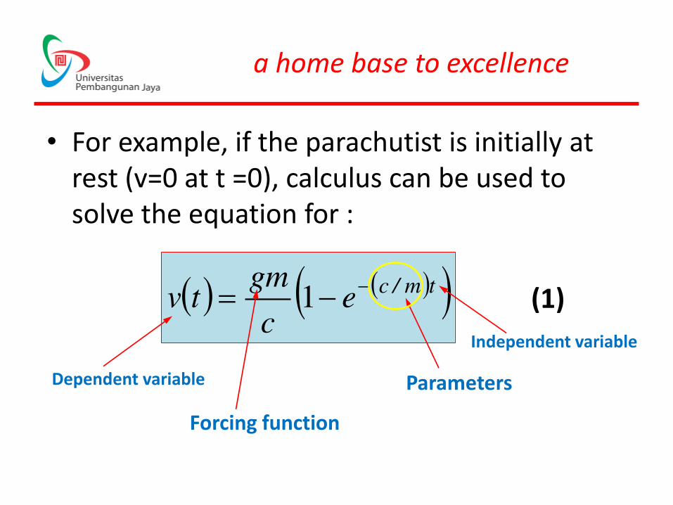
• For example, if the parachutist is initially at

rest (v=0 at t =0), calculus can be used to

solve the equation for :

tm/ce

c

gmtv

1

Dependent variable

Forcing function

Parameters

Independent variable

(1)


• Solution for differential equation cannot

always be solved analytically using simple

algebraic solution.

• The exact solution for differential equation

can be solved using calculus or by

approximation using numerical methods.


Example 1 :

A parachutist of mass 68,1 kg

jumps out a stationary hot air

balloon. Compute velocity prior to

opening the chute. The drag

coefficient is equal to 12.5 kg/s.

Inserting the parameters into the

equation (1) above yields :

t,t,/,e,e

,

,,tv

183550168512 139531512

16889


• As mentioned previously,

numerical methods are those in

which the mathematical problem

is reformulated so it can be solved

by arithmetic operations.

• This can be illustrated for

Ne to ’s second law by realizing

that the time rate of change of

velocity can be approximated by

ii

ii

tt

tvtv

t

v

dt

dv

1

1(2)

t

vlim

dt

dv

t

0

Remember :


• Equation (2) is called a finite divided

difference approximation of the derivative at

time ti. Substitute (2) to (1) give :

• Rearranged to yield :

i

ii

ii tvm

cg

tt

tvtv

1

1

iiiii tttvm

cgtvtv

11

this app oa h is fo all alled Eule ’s ethod

(3)


Example 2 :

Perform the same computation as in Example 1 but use

Equation (3) to compute the velocity. Employ a step size of 2 s

for the calculation.

At the start of the computation (ti =0), the velocity of the

parachutist is zero.

Using this information and the parameter values from Example

1, Eq. (3) can be used to compute velocity at ti+1=2s:

m/s 601920168

5128902 ,

,

,,tv


Example 2 :

For the next interval (from t =2to 4 s), the computation is

repeated, with the result :

m/s 003226019

168

5128960194 ,,

,

,,,tv


Approximations and Round-Off Errors • Although the numerical technique yielded estimates that

were close to the exact analytical solution, there was a discrepancy, or error, because the numerical method involved an approximation.

• Actually, we were fortunate in that case because the availability of an analytical solution allowed us to compute the error exactly.

• For many applied engineering problems, we cannot obtain analytical solutions.

• Therefore, we cannot compute exactly the errors associated with our numerical methods.

• In these cases, we must settle for approximations or estimates of the errors


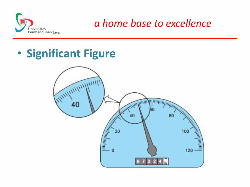
• Significant Figure


• The significant digits of a number are those that can be used with confidence.

• They correspond to the number of certain digits plus one estimated digit.

• For example, the speedometer and the odometer yield readings of three and seven significant figures, respectively.

• For the speedometer, the two certain digits are 48. It is conventional to set the estimated digit at one-half of the smallest scale division on the measurement device. Thus the speedometer reading would consist of the three significant figures: 48.5.

• In a similar fashion, the odometer would yield a seven-significant-figure reading of 87,324.45


The concept of significant figures has two important implications for our

study of numerical methods:

1. As introduced in the falling parachutist problem, numerical methods

yield approximate results. We must, therefore, develop criteria to

specify how confident we are in our approximate result. One way to do

this is in terms of significant figures. For example, we might decide that

our approximation is acceptable if it is correct to four significant figures.

2. Although ua tities su h as π, e, o √ ep ese t specific quantities,

they cannot be expressed exactly by a limited number of digits. For

e a ple, π= . ... Because computers retain only a finite number of significant figures, such

numbers can never be represented exactly. The omission of the remaining

significant figures is called round-off error.


• Accuracy. How close is a computed or measured value to the true value

• Precision (or reproducibility). How close is a computed or measured value to previously Computed or measured values.

• Inaccuracy (or bias). A systematic deviation from the actual value

• Imprecision (or uncertainty). Magnitude of scatter.

(a) Inaccurate and imprecise; (b) accurate and

imprecise; (c) inaccurate and precise; (d)

accurate and precise.


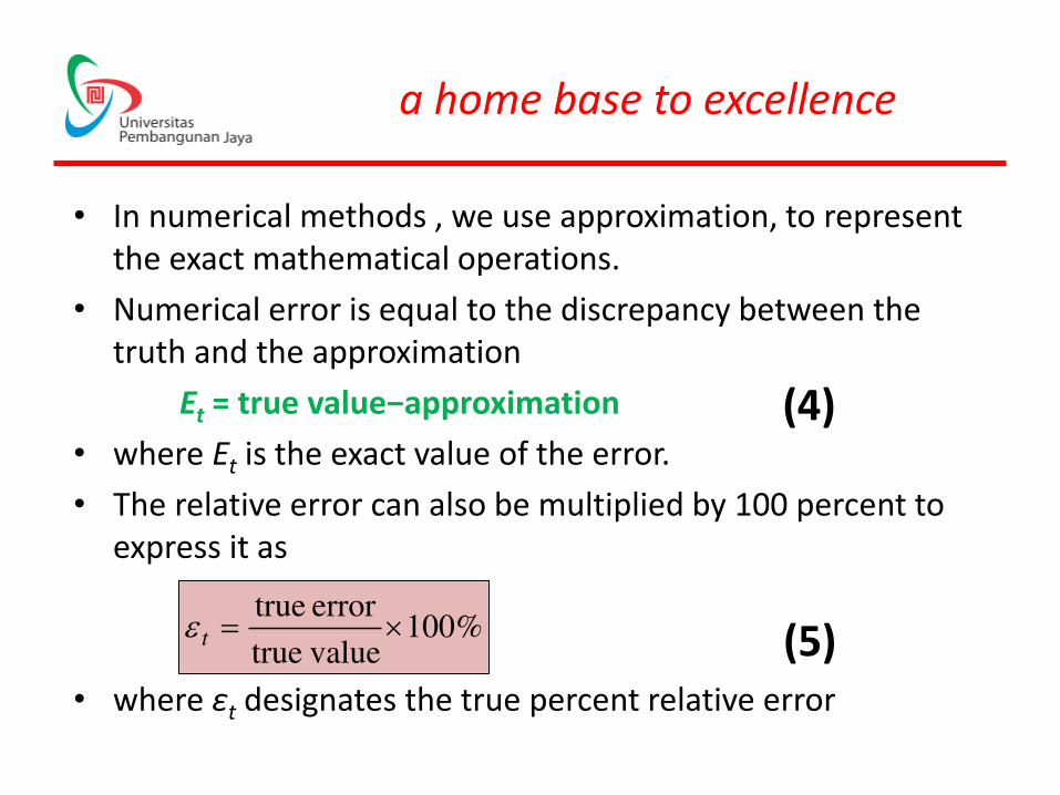
• In numerical methods , we use approximation, to represent

the exact mathematical operations.

• Numerical error is equal to the discrepancy between the

truth and the approximation

Et = true alue−approximation

• where Et is the exact value of the error.

• The relative error can also be multiplied by 100 percent to

express it as

• where εt designates the true percent relative error

(4)

%t 100 valuetrue

error true (5)


Example 3 :

Suppose that you have the task of measuring

the lengths of a bridge and a rivet and come up

with 9999 and 9 cm, respectively. If the true

values are 10,000 and 10 cm, respectively,

compute (a) the true error and (b) the true

percent relative error for each case.


If we cannot solved the problem

analytically to get the true value, how to

calculate its true error?

• We normalize the error to approximate value.

• Numerical methods use iterative approach to

compute answers.

• A present approximation is made on the basis

of a previous approximation.


• Percent relative error, a

• The signs of Eqs. (6) may be either positive or negative.

• Often, when performing computations, we may not be concerned with the sign of the error, but we are interested in whether the percent absolute value is lower than a p espe ified pe e t tole a e εs.

• Therefore, it is often useful to employ the absolute value of Eqs. (6).

• For such cases, the computation is repeated until

|εa|< εs

%a 100ionapproximatcurrent

ionapproximat previous-ionapproximatcurrent (6)


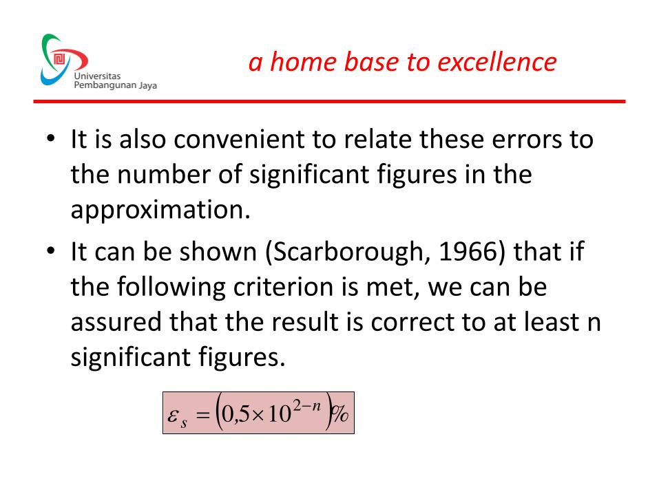
• It is also convenient to relate these errors to

the number of significant figures in the

approximation.

• It can be shown (Scarborough, 1966) that if

the following criterion is met, we can be

assured that the result is correct to at least n

significant figures.

%,n

s 21050


Example 4 :

• In mathematics, functions can often be represented by

infinite series. For example, the exponential function can be

computed using Maclaurin series expansion

• Estimate the value of e0,5.

• Add terms until the absolute value of the approximate error

estimate εa falls below a pre specified error criterion εs

conforming to three significant figures.

• Note that the true value is e0.5= . 4 …

!!321

32

n

x...

xxxe

nx

Documents

a home base to excellence - OPENCOURSEWARE …ocw.upj.ac.id/files/Slide-TSP303-Analisis-Numerik-Pemrograman-TSP... · Ujian Tengah Semester : 30% ... a home base to excellence