A HIGH-RESOLUTION SPECTROSCOPIC SEARCH FOR THE …

The Astrophysical Journal, 774:99 (19pp), 2013 September 10 doi:10.1088/0004-637X/774/2/99C© 2013. The American Astronomical Society. All rights reserved. Printed in the U.S.A.

A HIGH-RESOLUTION SPECTROSCOPIC SEARCH FOR THE REMAININGDONOR FOR TYCHO’S SUPERNOVA

Wolfgang E. Kerzendorf1,2, David Yong1, Brian P. Schmidt1, Joshua D. Simon3, C. Simon Jeffery4, Jay Anderson5,Philipp Podsiadlowski6, Avishay Gal-Yam7, Jeffrey M. Silverman8,9, Alexei V. Filippenko8, Ken’ichi Nomoto10,

Simon J. Murphy1, Michael S. Bessell1, Kim A. Venn11, and Ryan J. Foley121 Research School of Astronomy and Astrophysics, Mount Stromlo Observatory, Cotter Road, Weston Creek, ACT 2611, Australia; [email protected]

2 Department of Astronomy and Astrophysics, University of Toronto, 50 Saint George Street, Toronto, ON M5S 3H4, Canada3 The Observatories of the Carnegie Institution for Science, 813 Santa Barbara Street, Pasadena, CA 91101, USA

4 Armagh Observatory, College Hill, Armagh BT61 9DG, UK5 Space Telescope Science Institute, Baltimore, MD 21218, USA

6 Department of Astrophysics, University of Oxford, Oxford, OX1 3RH, UK7 Benoziyo Center for Astrophysics, Faculty of Physics, The Weizmann Institute of Science, Rehovot 76100, Israel

8 Department of Astronomy, University of California, Berkeley, CA 94720-3411, USA9 Department of Astronomy, University of Texas, Austin, TX 78712-0259, USA

10 Kavli Institute for the Physics and Mathematics of the Universe, The University of Tokyo, 5-1-5 Kashiwanoha, Kashiwa, Chiba 277-8583, Japan11 Department of Physics and Astronomy, University of Victoria, Elliott Building, 3800 Finnerty Road, Victoria, BC V8P 5C2, Canada

12 Harvard-Smithsonian Center for Astrophysics, 60 Garden Street, Cambridge, MA 02138, USAReceived 2012 April 16; accepted 2013 April 9; published 2013 August 21

ABSTRACT

In this paper, we report on our analysis using Hubble Space Telescope astrometry and Keck-I HIRES spectroscopyof the central six stars of Tycho’s supernova remnant (SN 1572). With these data, we measured the propermotions, radial velocities, rotational velocities, and chemical abundances of these objects. Regarding the chemicalabundances, we do not confirm the unusually high [Ni/Fe] ratio previously reported for Tycho-G. Rather, wefind that for all metrics in all stars, none exhibit the characteristics expected from traditional Type Ia supernovasingle-degenerate-scenario calculations. The only possible exception is Tycho-B, a rare, metal-poor A-type star;however, we are unable to find a suitable scenario for it. Thus, we suggest that SN 1572 cannot be explained by thestandard single-degenerate model.

Key words: ISM: supernova remnants – supernovae: individual (SN1572)

Online-only material: color figures

1. INTRODUCTION

Type Ia supernovae (SNe Ia) are of great interest. They rep-resent some of the most extreme physical situations in stel-lar astronomy, control the chemical evolution of galaxies andthe universe at intermediate to late times by producing largeamounts of iron-group elements, and are uniquely powerfulcosmic distance probes. But despite their wide-ranging signifi-cance, fundamental uncertainties remain around the progenitorsof these cataclysmic events.

There is a general consensus that SNe Ia are caused by thedeflagration/detonation of a carbon–oxygen white dwarf whichis accreting material from a binary companion. Scenarios existwhere the explosion can be initiated from a detonation on thesurface of the star (Livne & Arnett 1995; Fink et al. 2010),through runaway carbon burning in the white dwarf’s interior,or through a cataclysmic merger of objects.

Observationally, two main models for this accretionprocess can be identified. The single-degenerate scenario(SD-scenario) sees the accretion process occurring throughRoche-lobe overflow (RLOF) of a close nondegenerate com-panion (also known as a donor star). This companion, which hasundergone common-envelope evolution with the white dwarf,can be a helium, main-sequence, subgiant, or red giant star. Inall cases, the donor star should survive the explosion (except forpossibly in the case of the helium-star donor; R. Pakmor 2012,private communication) and remain visible post-explosion.

The second scenario is the dynamical merger of two whitedwarfs, known as the double-degenerate scenario. In this

scenario, the coevolution of two stars eventually leads to a closebinary of two white dwarfs, which are able, through the emis-sion of gravitational radiation, to merge over a wide range oftimes after the initial formation of the system. In most cases,this would leave no remaining star (e.g., Pakmor et al. 2010).

Both scenarios have support in observations and theory. Thedetection of circumstellar material around certain SNe Ia (Patatet al. 2007; Simon et al. 2009; Sternberg et al. 2011; Foley et al.2012) provides evidence for the SD-scenario. On the other hand,the lack of substantial hydrogen in the majority of other SNe Ia(Leonard 2007) poses a challenge to the SD-scenario.

Kasen (2010) suggests that the interaction of the shock wavewith the nondegenerate companion should result in a light excessat early times of an SN Ia light curve, which depends on theviewing angle and the companion radius. Such an excess hasnot yet been observed (Hayden et al. 2010; Tucker 2011; Biancoet al. 2011; Ganeshalingam et al. 2011), which is at odds withred giant companions forming the majority of SNe Ia. Justham(2011), Di Stefano et al. (2011), and Hachisu et al. (2012a,2012b), however, have suggested a scenario where the whitedwarf is spinning and thus can accrete above the Chandrasekharlimit. The explosion would only occur once the white dwarf hadspun down sufficiently, which would give the red giant a chanceto evolve and would not require the detection of the early excessin the light curve in a red giant progenitor scenario.

Population-synthesis calculations are challenging, with var-ious authors getting different results for the same inputs.However, there is a general trend from these calculationsthat neither single-degenerate nor double-degenerate stars can

1

http://dx.doi.org/10.1088/0004-637X/774/2/99

mailto:[email protected]

The Astrophysical Journal, 774:99 (19pp), 2013 September 10 Kerzendorf et al.

provide enough systems to explain the observed SN Ia rate (Han2008; Ruiter et al. 2009; Mennekens et al. 2010; Yu & Jeffery2010). Several authors suggest that the population might com-prise both single-degenerate and double-degenerate systems.

The physics of white-dwarf mergers is challenging to simulatenumerically, but in the simplest calculations, these mergers leadto the formation of a neutron star via electron capture, rather thanto a thermonuclear explosion (Saio & Nomoto 1985). Recently,Pakmor et al. (2010) have shown that for certain parameters(white-dwarf binaries with a mass ratio very close to one)the merger may explain subluminous supernovae (SNe; e.g.,SN 1991bg; see Filippenko 1997, for a review), although Danet al. (2011) note that the initial conditions of the system maychange these conclusions.

SN 2011fe was detected only ∼11 hr after the explosion(Nugent et al. 2011), and (with a distance of 6.4 Mpc) is oneof the closest SNe Ia ever found. Nugent et al. (2011) andBrown et al. (2012) have not found any early-time light-curveexcess predicted by Kasen (2010), and thus rule out a red giantdonor. Radio and X-ray observations by Horesh et al. (2012)show no strong signs of pre-explosion outflows, which againcontradicts a red giant scenario for SN 2011fe. Additional radiomeasurements by Chomiuk et al. (2012) suggest a low densityaround SN 2011fe, which is at odds with many conventionalSD-scenarios. Li et al. (2011) have searched pre-explosionarchival images and can also rule out luminous red giants andalmost all helium stars as donors. In addition, Bloom et al.(2012) have used images believed to have been taken 4 hrpost-explosion and suggest the companion radius to be lessthan 0.1 R�. Most of these results are consistent with a main-sequence companion or a white-dwarf companion.

Because it is very difficult to obtain robust constraintson the progenitor system in the immediate aftermath of a1051 erg explosion, an alternative is to study somewhat olderand more nearby SNe that can be observed in great detail.Ruiz-Lapuente et al. (2004, henceforth RP04) have tried todirectly detect donor stars in old and nearby SN Ia remnantswithin the Milky Way. They have identified two historicalGalactic SNe well suited to this task—SN 1006 and SN 1572(Tycho’s SN). Both remnants are young (1000 and 440 yr old,respectively), closeby (2.2 ± 0.08 kpc, Winkler et al. 2003;2.8 ± 0.8 kpc, Ruiz-Lapuente 2004), almost certainly SNe Iafrom their observational signatures (Badenes et al. 2006; Ruiz-Lapuente 2004; Krause et al. 2008; Rest et al. 2008), and notoverwhelmed by Galactic extinction. In this paper, we will focuson SN 1572.

RP04 investigated most bright stars in the central region of SN1572 and found a star with an unusual spatial motion (Tycho-Gby their nomenclature); they suggested this as a possible donorstar for SN 1572. While the star has an unusual spatial motioncompared to other stars in the field, its current location andproper motion place it on a significant distance from the centerof the supernova remnant (SNR)—a feature difficult to explainin connecting Tycho-G to SNR 1572.

In the case of RLOF, the time scale for synchronization ofthe orbit by tidal interaction due to dissipation processes isshort enough to ensure almost synchronous rotation in spite ofmass-loss. This results in an unusually large rotational velocity,related to the orbital velocity of the binary system, and itmight be used to single out possible donor stars from nearbyunrelated stars. Kerzendorf et al. (2009, henceforth WEK09)investigated the rotation of Tycho-G but found no excessrotational velocity compared to a normal star. A comparison of

WEK09’s measurements of Tycho-G, including a revised radialvelocity vrad, with Galactic kinematic models showed that itis statistically consistent with an unrelated thick/thin-disk star.However, WEK09 were able to provide an a priori unlikelydonor-star scenario, where the star was able to lose its rotationalsignature.

Gonzalez Hernandez et al. (2009, henceforth GH09) analyzeda spectrum of Tycho-G observed with the High ResolutionEchelle Spectrometer (HIRES; Vogt et al. 1994) instrumenton the Keck-I 10 m telescope, finding a vrad value consistentwith WEK09’s revised vrad. They also measured the stellarparameters and metallicity of Tycho-G, concluding that it hasan unusually high nickel abundance, which they claim can beattributed to the accretion of ejecta material on the donor starduring the explosion.

In this paper, we analyze HIRES spectra of the six bright starsnear the center of SNR 1572. These spectra were taken as part ofthe same program that obtained the data used by GH09, and weindependently reanalyze the Tycho-G spectrum in our program.We describe the observational data and our data-reductionprocedures in Section 2. Section 3 is divided into six subsectionsdetailing the measurements of proper motion, radial velocity,rotation, stellar parameters, and abundances, and we provide adetailed comparison between our and GH09’s measurements ofTycho-G. In Section 4, we analyze the measurements of eachstar to investigate its potential association with SNR 1572, andwe present our conclusions in Section 5.

2. OBSERVATIONS AND DATA REDUCTION

We obtained spectra with the HIRES spectrograph on theKeck-I telescope on Mauna Kea. The observations were madeon 2006 September 10 and 2006 October 11 UT. Slits B5 and C1(width 0.′′86; B5 length 3.′′5, C1 length 7.′′0) were used, resultingin wavelength coverage of 3930–5330 Å, 5380–6920 Å, and6980–8560 Å with R = λ/Δλ ≈ 50,000, providing us withthe necessary spectral resolution and wavelength coverage todetermine stellar parameters.

The spectra were reduced using the makee package. All spec-tra were corrected to heliocentric velocities, using the makeesky-line method. The spectra were not corrected for telluricabsorption lines, but only regions known to be free fromtelluric contamination were used in the analysis to derivethe stellar parameters. The final exposure times of the com-bined spectra for each candidate and the signal-to-noise ratio(S/N) at 5800–5900 Å are shown in Table 1. Finally, we nor-malized the spectrum using the iraf13 task continuum. Wenote that Tycho-C and Tycho-D were observed on the sameslit (C1); they are separated by 2.′′1, and the seeing was ∼0.′′8,with Tycho-C being roughly five times brighter than Tycho-D.All HIRES spectra (except Tycho-B) are available for down-load in the WISEREP repository (http://www.weizmann.ac.il/astrophysics/wiserep; Yaron & Gal-Yam 2012).

In addition, we obtained low-resolution spectra (R ≈ 1200)of Tycho-B with the dual-arm Low-Resolution Imaging Spec-trometer (LRIS; Oke et al. 1995) mounted on the Keck-I tele-scope. The data were taken on 2010 November 7 UT, using onlythe blue arm with the 600/4000 grism and the 1′′wide slit. Thisresulted in a wavelength coverage of 3200–5600 Å. These data

13 IRAF is distributed by the National Optical Astronomy Observatory, whichis operated by the Association of Universities for Research in Astronomy, Inc.,under cooperative agreement with the National Science Foundation.

2

http://www.weizmann.ac.il/astrophysics/wiserep

http://www.weizmann.ac.il/astrophysics/wiserep


Table 1Observations

Tycho α(J2000) δ(J2000) Date Slit texp V a S/Nb

(Name) (hh:mm:ss.ss) (dd:mm:ss.ss) (dd/mm/yy) (minutes) (mag)

A 00:25:19.73 +64:08:19.60 10/09/06 B5 15 13, 29 ∼48B 00:25:19.95 +64:08:17.11 10/09/06 B5 20 15.41 ∼45C 00:25:20.40 +64:08:12.32 11/10/06 C1 180 19.06c ∼8D 00:25:20.60 +64:08:10.82 11/10/06 C1 180 20.70 ∼3E 00:25:18.29 +64:08:16.12 11/10/06 C1 150 19.79 ∼9G 00:25:23.58 +64:08:02.06 10/09/06 & 11/10/06 B5&C1 400 18.71 ∼25

Notes.a Magnitudes from RP04.b The S/N value was obtained by measuring the root mean square of the pixels (each resolution element is sampled by two pixels) in continuumregions near 5800–5900 Å. For the purposes of measuring the stellar parameters, the spectrum was convolved so that the S/N increased by afactor of 2.24.c RP04 notes that this is an unresolved pair with a brighter bluer component (V = 19.38 mag) and a fainter redder component (V =20.53 mag).

were taken to obtain a precise measurement of the surface grav-ity for Tycho-B using the observed Balmer decrement (Bessell2007).

The spectrum of Tycho-B was reduced using standard tech-niques (e.g., Foley et al. 2003). Routine CCD processing andspectrum extraction were completed with iraf, and the datawere extracted with the optimal algorithm of Horne (1986). Weobtained the wavelength scale from low-order polynomial fits tothe calibration-lamp spectra. Small wavelength shifts were thenapplied to the data after measuring the offset by cross-correlatinga template sky to the night-sky lines that were extracted withthe star. Using our own idl routines, we fit a spectrophotomet-ric standard-star spectrum to the data in order to flux calibrateTycho-B and remove telluric lines (Horne 1986; Matheson et al.2000).

3. ANALYSIS

3.1. Astrometry

Proper motions can be used to identify potential donor starsbecause donor stars freely travel with their orbital velocity afterthe SN explosion disrupts the system. RP04 suggested Tycho-Gas a possible donor due to its unusually high values for boththe proper motion and the radial velocity. For this work, wemeasured proper motions for 201 stars within 1 arcmin of theremnant’s center. We used archival Hubble Space Telescope(HST) images for three different epochs (HST ProgramsGO-9729 and GO-10098; 2003 November, 2004 August, 2005May), each consisting of three depths with three exposures each(3 × 0.5 s, 3 × 10 s, 4 × 480 s) with the F555W filter using theAdvanced Camera for Surveys. The scale in each exposure is50 mas pixel−1. This data set results in a maximum baseline of18 months.

We used an image from the middle epoch (2004) to establisha reference frame and oriented the pixel coordinate system withthe equatorial system. We then applied a distortion correctionfor the F555W filter (Anderson & King 2006) and calculatedtransformations between all other images and the referenceimage. Next, we extracted the stellar positions in all frames(utilizing a library point-spread function that varies across thefield) and used the transformations between the images tocalculate the position of all stars in the reference coordinatesystem, with the overall uncertainty of each position estimated.Some faint stars were not detected in the shorter exposures and

were thus excluded from proper-motion measurements. In total,114 stars were used in the astrometric analysis.

For each star, we fit a linear regression for the stellar positionsover time in the pixel coordinates (which were aligned with theequatorial system). The x and y data were treated as independentmeasurements, with separate regressions solved for each axisdirection. Uncertainties were estimated using standard least-squares analysis and the individual uncertainty estimates of eachobject’s positions.

There are three J2000 measurements of the geometric centerof SN 1572 from different data sets. Reynoso et al. (1997)used Very Large Array data to find α = 00h25m14.s95, δ =+64◦08′05.′′7; Hughes (2000) used ROSAT data to measureα = 00h25m19.s0, δ = +64◦08′10′′; and Warren et al. (2005)used Chandra X-Ray Observatory data to get α = 00h25m19.s40,δ = 64◦08′13.′′98. We note that the X-ray centers agree ratherwell with a difference of less than 5′′, but the radio center islocated roughly 30′′ away from the X-ray centers. Thus, webelieve the uncertainty in the geometric center is rather large (ofthe order of 30′′).

Table 2 lists the proper motions and uncertainties of all starsmentioned by RP04 (19 stars) that were analyzed in this work,as well as the distance to the geometric X-ray center measuredby Chandra.

We note that Tycho-2 has a relatively high proper motion, butits position in the year 1572 was 67.′′95 away from the remnant’scenter, and we thus exclude it as a viable candidate for the donor.

In Figure 1, we compare the distribution of proper motions ofall measured stars with those of our candidates. All of the latterare reconcilable with a normal proper-motion distribution.

3.2. Radial Velocity

For the radial-velocity measurement, we first obtained well-calibrated wavelength solutions for our spectra. MAKEE per-forms an initial calibration of the wavelength using lamp spectraand then refines it by cross-correlating the night-sky lines foreach observation and determining minor offsets. Both scienceobjects and radial-velocity standards were reduced in the samefashion.

Each order of each star spectrum was then cross-correlatedusing the iraf task fxcor (Tonry & Davis 1979) with at least twoother radial-velocity standards (HR6349, HR6970, or HR1283)which had been observed on the same night. We measure theradial velocity of the standards and, comparing to the canonical

3


Table 2Proper Motions of Candidates

Tycho α(J2000) δ(J2000) μα μδ Δμα Δμδ μl μb r(Name) (hh:mm:ss.ss) (dd:mm:ss.ss) (mas yr−1) (mas yr−1) (mas yr−1) (′′)

B 0:25:19.97 64:08:17.1 −1.24 0.56 0.62 0.64 −1.17 0.68 4.86A 0:25:19.73 64:08:19.8 −0.09 −0.89 1.17 0.90 −0.18 −0.88 6.21A2 0:25:19.81 64:08:20.0 −0.71 −3.60 0.69 0.64 −1.07 −3.51 6.58C 0:25:20.38 64:08:12.2 −0.21 −2.52 0.65 0.65 −0.46 −2.48 6.66E 0:25:18.28 64:08:16.1 2.04 0.54 0.66 0.69 2.09 0.33 7.60D 0:25:20.62 64:08:10.8 −1.12 −1.99 1.01 0.86 −1.32 −1.87 8.601 0:25:16.66 64:08:12.5 −2.27 −1.37 1.60 1.15 −2.40 −1.14 18.00F 0:25:17.09 64:08:30.9 −4.41 0.20 0.70 0.71 −4.37 0.65 22.69J 0:25:15.08 64:08:05.9 −2.40 −0.25 0.62 0.62 −2.42 −0.00 29.44G 0:25:23.58 64:08:01.9 −2.50 −4.22 0.60 0.60 −2.91 −3.95 29.87R 0:25:15.51 64:08:35.4 0.28 0.24 0.89 0.80 0.30 0.21 33.23N 0:25:14.73 64:08:28.1 1.18 0.89 0.86 0.98 1.27 0.77 33.66U 0:25:19.24 64:07:37.9 0.01 −3.04 0.73 0.75 −0.30 −3.03 36.06Q 0:25:14.81 64:08:34.2 1.45 3.07 0.64 0.72 1.75 2.91 36.19T 0:25:14.58 64:07:55.0 −3.85 0.52 0.72 0.62 −3.77 0.91 36.78K 0:25:23.89 64:08:39.3 0.18 0.17 0.73 0.69 0.20 0.15 38.73L 0:25:24.30 64:08:40.5 0.16 −0.44 0.75 0.82 0.11 −0.45 41.59S 0:25:13.78 64:08:34.4 4.16 0.58 0.83 0.84 4.20 0.15 42.092 0:25:22.44 64:07:32.4 74.85 −4.43 0.82 0.83 74.05 −11.94 46.09

−4 −2 0 2 4μα [mas/yr]

−4

−2

0

2

4

μδ

[mas

/yr]

U

T

G

J

DC

1

EB

A2

N

F

Q

SR

K

L

A

Figure 1. Contours display the distribution of proper motions (68% and 95%probability) for all stars measured toward the Tycho SNR, excluding the namedstars. We show the location of the candidate stars and their uncertainties on topof this distribution. Tycho-2 (called HP-1 in WEK09) is not shown in this figureas it is an extreme outlier with μα = 75 mas yr−1 and μδ = −4.4 mas yr−1; it isalso at a large distance from the remnant’s geometric center (46′′). In addition,the dashed contour represents the 1σ level of the thick disk proper motionaccording to the Besancon model. Using the same Besancon model as a proxy,we estimate the contamination of the HST sample with foreground objects (lessthan 2 kpc) to be roughly 30%.

values (Stefanik et al. 1999), we obtain a systematic errorof ∼1 km s−1, which is negligible compared to the measuredvelocities.

The radial velocity of Tycho-B was measured in the course ofdetermining the stellar parameters of Tycho-B with the stellarparameter fitting package sfit (Jeffery et al. 2001). The sfitresult consistently gives vhelio = −52 km s−1 for different stellarparameters with an uncertainty of ∼2 km s−1.

In Table 3, we list all of the radial velocities both in aheliocentric frame and a local standard of rest (LSR) frame.We will be referring to the heliocentric measurements hence-forth. The listed uncertainty is the standard deviation of the

Table 3Radial Velocities of Candidates

Tycho Date vhelio vLSR σ

(Name) (dd/mm/yy) (dd:mm:ss.ss) (km s−1) (km s−1)

Tycho-A 09/09/06 −36.79 −28.50 0.23Tycho-B 09/09/06 −52.70 −44.41 ∼2Tycho-C 11/10/06 −58.78 −50.49 0.75Tycho-D 11/10/06 −58.93 −50.64 0.78Tycho-Ea 11/10/06 −64.20 −55.91 0.27Tycho-G 09/09/06 −87.12 −78.83 0.25Tycho-G 11/10/06 −87.51 −79.22 0.78

Note. a There seems to be a discrepancy between RP04 and this work(measurement by RP04 vLSR −26 km s−1), which might be a possible hintof a binary system.

radial-velocity measurement of all orders added in quadratureto the error of the radial-velocity standards.

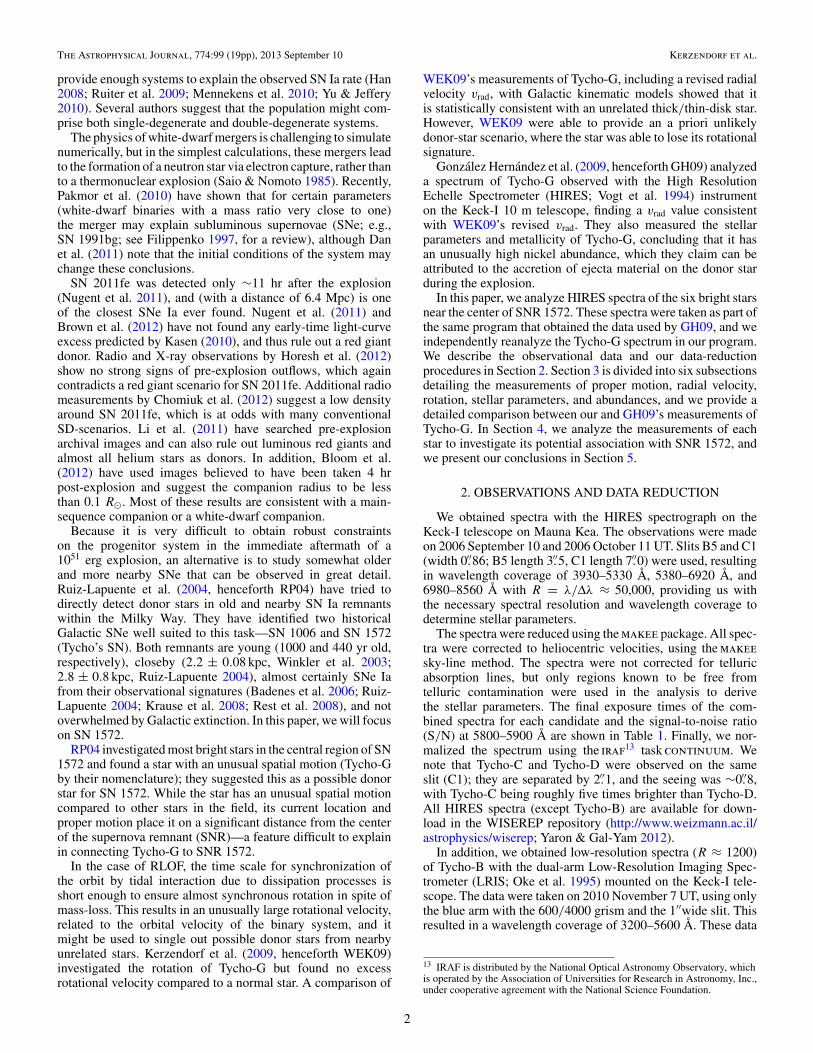
In Figure 2, we compare the radial velocity of our sample starsto the radial velocities of stars in the direction of Tycho’s SNRusing the Besancon model (Robin et al. 2003). The distancesas well as their uncertainties are taken from Section 3.6. Thecandidates’ radial velocities are all typical for their distances.Finally, we note that the measurement of Tycho-G is consistentwith the results of WEK09 and GH09.

3.3. Rotational Velocity

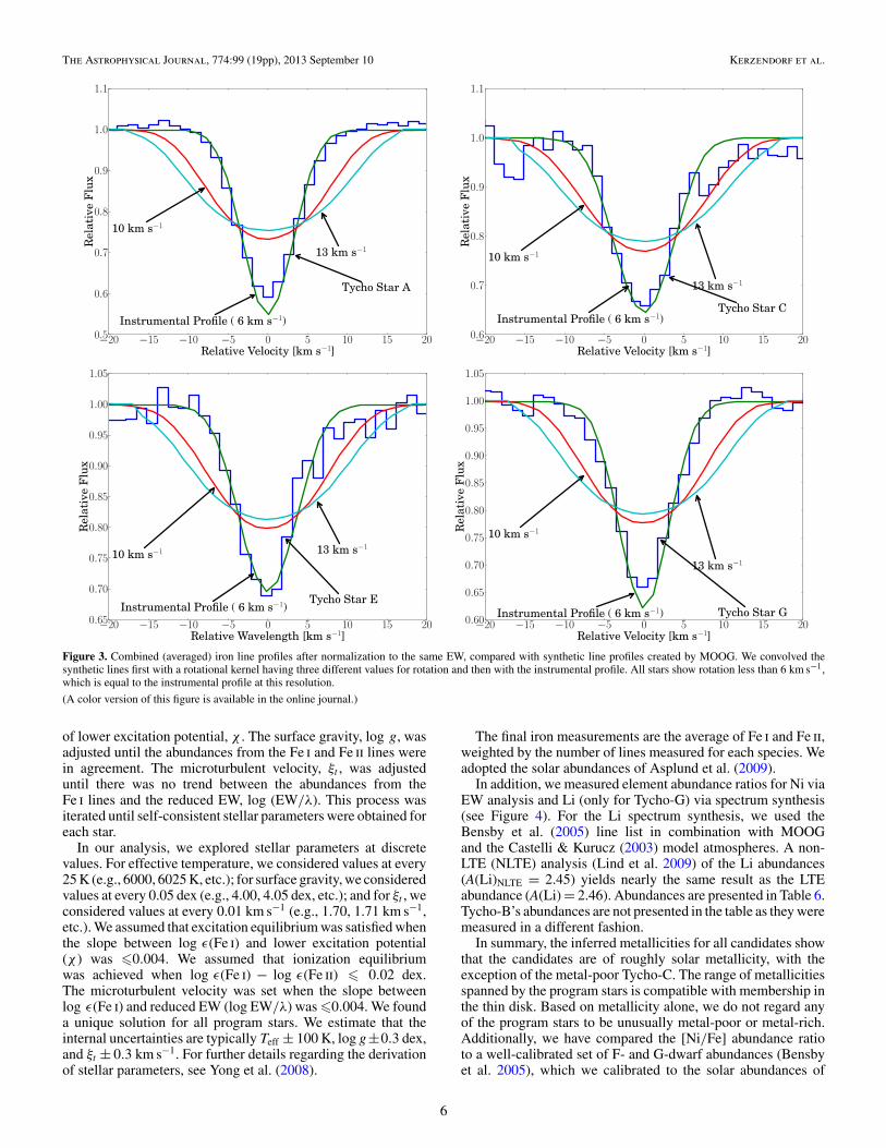
We have measured the projected rotational velocities(vrot sin i) of all stars except Tycho-B in the fashion describedby WEK09. We selected several unblended and strong (but notsaturated) Fe i lines in the stellar spectra and averaged themafter shifting to the same wavelength and scaling to the sameequivalent width (EW). This was done to improve the S/N forthe faint stars as well as to provide consistency throughout allstars.

As a reference, we created three synthetic spectra for eachstar (one broadened only with the instrumental profile, theothers with the instrumental profile and a vrot sin i of 10 and13 km s−1) with the 2010 version of MOOG (Sneden 1973),

4


0 2 4 6 8 10 12Distance [kpc]

−150

−100

−50

0

v rad

[km

s−1 ] AA

BBCC

EE

GG

Figure 2. Contours indicating the 1σ , 2σ , and 3σ levels of the distance and radial velocity using the Besancon Model (Robin et al. 2003) with ∼ 60,000 stars in thedirection of SN 1572 (only including stars with 10 < V < 20 mag and with a metallicity of [Fe/H] > −1 for the filled contours and [Fe/H] > −0.2 for the dashedcontours). We have overplotted our candidate stars with error bars. One should note that the uncertainties in distance are a marginalized approximation of the error;the proper error surfaces can be seen in Figure 12. The vertical gray shade illustrates the error range for the distance to SNR 1572.

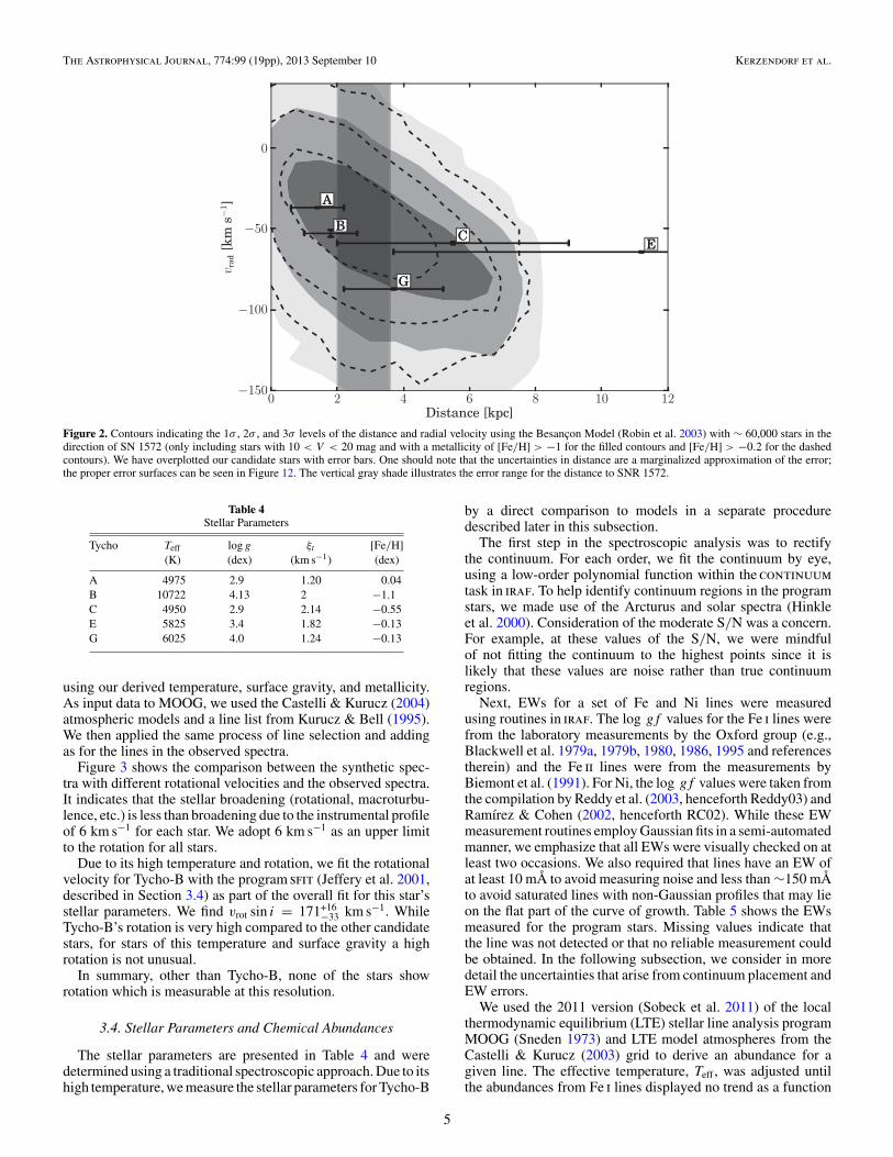
Table 4Stellar Parameters

Tycho Teff log g ξt [Fe/H](K) (dex) (km s−1) (dex)

A 4975 2.9 1.20 0.04B 10722 4.13 2 −1.1C 4950 2.9 2.14 −0.55E 5825 3.4 1.82 −0.13G 6025 4.0 1.24 −0.13

using our derived temperature, surface gravity, and metallicity.As input data to MOOG, we used the Castelli & Kurucz (2004)atmospheric models and a line list from Kurucz & Bell (1995).We then applied the same process of line selection and addingas for the lines in the observed spectra.

Figure 3 shows the comparison between the synthetic spec-tra with different rotational velocities and the observed spectra.It indicates that the stellar broadening (rotational, macroturbu-lence, etc.) is less than broadening due to the instrumental profileof 6 km s−1 for each star. We adopt 6 km s−1 as an upper limitto the rotation for all stars.

Due to its high temperature and rotation, we fit the rotationalvelocity for Tycho-B with the program sfit (Jeffery et al. 2001,described in Section 3.4) as part of the overall fit for this star’sstellar parameters. We find vrot sin i = 171+16

−33 km s−1. WhileTycho-B’s rotation is very high compared to the other candidatestars, for stars of this temperature and surface gravity a highrotation is not unusual.

In summary, other than Tycho-B, none of the stars showrotation which is measurable at this resolution.

3.4. Stellar Parameters and Chemical Abundances

The stellar parameters are presented in Table 4 and weredetermined using a traditional spectroscopic approach. Due to itshigh temperature, we measure the stellar parameters for Tycho-B

by a direct comparison to models in a separate proceduredescribed later in this subsection.

The first step in the spectroscopic analysis was to rectifythe continuum. For each order, we fit the continuum by eye,using a low-order polynomial function within the continuumtask in iraf. To help identify continuum regions in the programstars, we made use of the Arcturus and solar spectra (Hinkleet al. 2000). Consideration of the moderate S/N was a concern.For example, at these values of the S/N, we were mindfulof not fitting the continuum to the highest points since it islikely that these values are noise rather than true continuumregions.

Next, EWs for a set of Fe and Ni lines were measuredusing routines in iraf. The log gf values for the Fe i lines werefrom the laboratory measurements by the Oxford group (e.g.,Blackwell et al. 1979a, 1979b, 1980, 1986, 1995 and referencestherein) and the Fe ii lines were from the measurements byBiemont et al. (1991). For Ni, the log gf values were taken fromthe compilation by Reddy et al. (2003, henceforth Reddy03) andRamırez & Cohen (2002, henceforth RC02). While these EWmeasurement routines employ Gaussian fits in a semi-automatedmanner, we emphasize that all EWs were visually checked on atleast two occasions. We also required that lines have an EW ofat least 10 mÅ to avoid measuring noise and less than ∼150 mÅto avoid saturated lines with non-Gaussian profiles that may lieon the flat part of the curve of growth. Table 5 shows the EWsmeasured for the program stars. Missing values indicate thatthe line was not detected or that no reliable measurement couldbe obtained. In the following subsection, we consider in moredetail the uncertainties that arise from continuum placement andEW errors.

We used the 2011 version (Sobeck et al. 2011) of the localthermodynamic equilibrium (LTE) stellar line analysis programMOOG (Sneden 1973) and LTE model atmospheres from theCastelli & Kurucz (2003) grid to derive an abundance for agiven line. The effective temperature, Teff , was adjusted untilthe abundances from Fe i lines displayed no trend as a function

5


−20 −15 −10 −5 0 5 10 15 20Relative Velocity [km s−1]

0.5

0.6

0.7

0.8

0.9

1.0

1.1R

elat

ive

Flu

x

Tycho Star A

Instrumental Profile ( 6 km s−1)

10 km s−1

13 km s−1


0.6

0.7

0.8

0.9

1.0

1.1

Rel

ativ

eF

lux

Tycho Star CInstrumental Profile ( 6 km s−1)

10 km s−1

13 km s−1

−20 −15 −10 −5 0 5 10 15 20Relative Wavelength [km s−1]

0.65

0.70

0.75

0.80

0.85

0.90

0.95

1.00

1.05

Rel

ativ

eF

lux

Tycho Star EInstrumental Profile ( 6 km s−1)

10 km s−1 13 km s−1


0.60

0.65

0.70

0.75

0.80

0.85

0.90

0.95

1.00

1.05

Rel

ativ

eF

lux

Tycho Star GInstrumental Profile ( 6 km s−1)

10 km s−1

13 km s−1

Figure 3. Combined (averaged) iron line profiles after normalization to the same EW, compared with synthetic line profiles created by MOOG. We convolved thesynthetic lines first with a rotational kernel having three different values for rotation and then with the instrumental profile. All stars show rotation less than 6 km s−1,which is equal to the instrumental profile at this resolution.

(A color version of this figure is available in the online journal.)

of lower excitation potential, χ . The surface gravity, log g, wasadjusted until the abundances from the Fe i and Fe ii lines werein agreement. The microturbulent velocity, ξt , was adjusteduntil there was no trend between the abundances from theFe i lines and the reduced EW, log (EW/λ). This process wasiterated until self-consistent stellar parameters were obtained foreach star.

In our analysis, we explored stellar parameters at discretevalues. For effective temperature, we considered values at every25 K (e.g., 6000, 6025 K, etc.); for surface gravity, we consideredvalues at every 0.05 dex (e.g., 4.00, 4.05 dex, etc.); and for ξt , weconsidered values at every 0.01 km s−1 (e.g., 1.70, 1.71 km s−1,etc.). We assumed that excitation equilibrium was satisfied whenthe slope between log ε(Fe i) and lower excitation potential(χ ) was �0.004. We assumed that ionization equilibriumwas achieved when log ε(Fe i) − log ε(Fe ii) � 0.02 dex.The microturbulent velocity was set when the slope betweenlog ε(Fe i) and reduced EW (log EW/λ) was �0.004. We founda unique solution for all program stars. We estimate that theinternal uncertainties are typically Teff ± 100 K, log g±0.3 dex,and ξt ± 0.3 km s−1. For further details regarding the derivationof stellar parameters, see Yong et al. (2008).

The final iron measurements are the average of Fe i and Fe ii,weighted by the number of lines measured for each species. Weadopted the solar abundances of Asplund et al. (2009).

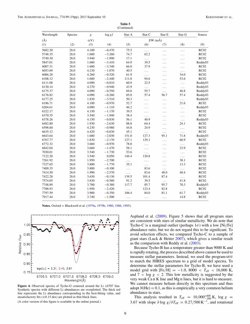
In addition, we measured element abundance ratios for Ni viaEW analysis and Li (only for Tycho-G) via spectrum synthesis(see Figure 4). For the Li spectrum synthesis, we used theBensby et al. (2005) line list in combination with MOOGand the Castelli & Kurucz (2003) model atmospheres. A non-LTE (NLTE) analysis (Lind et al. 2009) of the Li abundances(A(Li)NLTE = 2.45) yields nearly the same result as the LTEabundance (A(Li) = 2.46). Abundances are presented in Table 6.Tycho-B’s abundances are not presented in the table as they weremeasured in a different fashion.

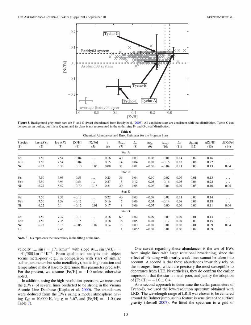
In summary, the inferred metallicities for all candidates showthat the candidates are of roughly solar metallicity, with theexception of the metal-poor Tycho-C. The range of metallicitiesspanned by the program stars is compatible with membership inthe thin disk. Based on metallicity alone, we do not regard anyof the program stars to be unusually metal-poor or metal-rich.Additionally, we have compared the [Ni/Fe] abundance ratioto a well-calibrated set of F- and G-dwarf abundances (Bensbyet al. 2005), which we calibrated to the solar abundances of

6


Table 5Line List and Equivalent Width Measurements

Wavelength Species χ log gf Star A Star C Star E Star G Source

(Å) (eV) EW (mÅ)(1) (2) (3) (4) (5) (6) (7) (8) (9)

4602.00 26.0 1.607 −3.154 114.8 . . . . . . . . . Oxford4733.59 26.0 1.484 −2.987 . . . . . . 102.3 85.4 Oxford4802.88 26.0 3.692 −1.531 91.0 96.0 . . . 64.8 Oxford4848.88 26.0 2.277 −3.154 . . . 85.9 . . . . . . Oxford4930.31 26.0 3.957 −1.264 . . . . . . . . . 57.8 Oxford4962.57 26.0 4.175 −1.199 77.5 . . . . . . . . . Oxford5014.94 26.0 3.940 −0.320 . . . . . . . . . 106.8 Oxford5044.21 26.0 2.849 −2.034 109.1 . . . . . . 67.2 Oxford5049.82 26.0 2.277 −1.372 . . . . . . . . . 117.8 Oxford5054.64 26.0 3.637 −1.938 70.8 . . . . . . 30.4 Oxford5083.34 26.0 0.957 −2.958 . . . . . . . . . 96.2 Oxford5141.74 26.0 2.422 −2.001 123.9 . . . . . . 85.4 Oxford5151.91 26.0 1.010 −3.322 . . . . . . . . . 85.0 Oxford5166.28 26.0 0.000 −4.195 . . . . . . 111.6 . . . Oxford5194.94 26.0 1.556 −2.090 . . . . . . . . . 113.8 Oxford5198.71 26.0 2.221 −2.135 . . . . . . . . . 92.1 Oxford5217.39 26.0 3.209 −1.179 . . . . . . 123.7 81.9 Oxford5223.19 26.0 3.632 −1.800 58.5 . . . 33.9 27.7 Oxford5225.52 26.0 0.110 −4.789 . . . . . . 82.3 65.6 Oxford5242.49 26.0 3.632 −0.984 113.9 . . . 110.6 69.8 Oxford5247.05 26.0 0.087 −4.946 . . . . . . 76.6 55.5 Oxford5250.21 26.0 0.121 −4.938 . . . . . . . . . 59.9 Oxford5253.46 26.0 3.281 −1.630 . . . . . . . . . 62.4 Oxford5412.80 26.0 4.431 −1.783 38.2 . . . . . . . . . Oxford5491.84 26.0 4.183 −2.253 36.9 . . . . . . . . . Oxford5497.52 26.0 1.010 −2.849 . . . . . . 129.3 102.1 Oxford5501.46 26.0 0.957 −3.063 . . . . . . . . . 90.9 Oxford5506.78 26.0 0.989 −2.797 . . . . . . . . . 95.7 Oxford5525.54 26.0 4.227 −1.149 . . . . . . . . . 38.4 Oxford5569.62 26.0 3.414 −0.544 . . . . . . 123.1 113.4 Oxford5586.76 26.0 3.366 −0.161 . . . . . . 142.8 . . . Oxford5600.23 26.0 4.257 −1.486 . . . . . . . . . 44.2 Oxford5618.63 26.0 4.206 −1.292 80.1 . . . . . . 43.3 Oxford5661.35 26.0 4.281 −1.822 48.2 . . . . . . 18.0 Oxford5662.51 26.0 4.175 −0.590 115.6 . . . 79.1 69.5 Oxford5701.55 26.0 2.557 −2.216 . . . . . . 104.7 . . . Oxford5705.47 26.0 4.298 −1.421 78.9 69.5 . . . . . . Oxford5741.85 26.0 4.253 −1.689 58.0 . . . . . . . . . Oxford5753.12 26.0 4.257 −0.705 . . . . . . . . . 52.0 Oxford5775.08 26.0 4.217 −1.314 82.3 73.0 . . . 34.5 Oxford5778.45 26.0 2.586 −3.481 55.5 58.5 . . . . . . Oxford5816.37 26.0 4.545 −0.618 . . . . . . . . . 66.5 Oxford5855.09 26.0 4.604 −1.547 43.1 . . . 17.1 . . . Oxford5909.97 26.0 3.209 −2.643 . . . 44.9 . . . 36.5 Oxford5916.25 26.0 2.452 −2.994 . . . 73.6 . . . 44.1 Oxford5956.69 26.0 0.858 −4.608 107.2 101.5 59.7 34.9 Oxford6012.21 26.0 2.221 −4.073 72.0 . . . . . . . . . Oxford6027.05 26.0 4.073 −1.106 100.3 79.9 . . . 63.3 Oxford6065.48 26.0 2.607 −1.530 . . . . . . 106.2 . . . Oxford6082.71 26.0 2.221 −3.573 . . . 61.6 . . . . . . Oxford6120.24 26.0 0.914 −5.970 33.9 . . . . . . . . . Oxford6136.62 26.0 2.452 −1.400 . . . . . . 145.6 . . . Oxford6136.99 26.0 2.196 −2.950 . . . . . . 71.7 . . . Oxford6151.62 26.0 2.174 −3.299 91.4 81.8 33.7 36.6 Oxford6165.36 26.0 4.140 −1.490 73.5 . . . 54.0 . . . Oxford6173.34 26.0 2.221 −2.880 115.1 . . . . . . 52.8 Oxford6180.20 26.0 2.725 −2.637 . . . 61.0 . . . 46.8 Oxford6200.31 26.0 2.607 −2.437 . . . 109.6 . . . 66.6 Oxford6219.28 26.0 2.196 −2.433 . . . 134.4 . . . 75.2 Oxford6229.23 26.0 2.843 −2.846 82.3 . . . 61.5 . . . Oxford6230.73 26.0 2.557 −1.281 . . . . . . . . . 109.9 Oxford6232.64 26.0 3.651 −1.283 114.5 129.1 106.6 65.3 Oxford6246.32 26.0 3.600 −0.894 . . . . . . . . . 106.2 Oxford6252.55 26.0 2.402 −1.687 . . . . . . . . . 100.8 Oxford

7


Table 5(Continued)


(Å) (eV) EW (mÅ)(1) (2) (3) (4) (5) (6) (7) (8) (9)

6265.13 26.0 2.174 −2.550 . . . . . . . . . 75.0 Oxford6270.22 26.0 2.856 −2.505 . . . 77.1 70.2 . . . Oxford6297.79 26.0 2.221 −2.740 120.6 115.1 93.5 61.7 Oxford6301.50 26.0 3.651 −0.766 . . . . . . 114.0 110.9 Oxford6322.69 26.0 2.586 −2.426 120.9 119.1 . . . . . . Oxford6335.33 26.0 2.196 −2.194 . . . . . . 116.4 75.0 Oxford6336.82 26.0 3.684 −0.916 . . . . . . . . . 69.1 Oxford6344.15 26.0 2.431 −2.923 . . . . . . . . . 48.4 Oxford6355.03 26.0 2.843 −2.403 . . . 101.7 93.4 64.4 Oxford6393.60 26.0 2.431 −1.469 . . . . . . 129.4 105.5 Oxford6408.02 26.0 3.684 −1.066 . . . 127.1 87.4 80.7 Oxford6411.65 26.0 3.651 −0.734 . . . . . . . . . 118.0 Oxford6430.84 26.0 2.174 −2.006 . . . . . . 135.0 102.5 Oxford6481.87 26.0 2.277 −2.984 113.2 . . . . . . 50.3 Oxford6498.94 26.0 0.957 −4.687 . . . 121.1 . . . 35.3 Oxford6574.23 26.0 0.989 −5.004 84.3 88.5 . . . 25.3 Oxford6575.02 26.0 2.586 −2.727 108.2 115.3 . . . 51.0 Oxford6592.91 26.0 2.725 −1.490 . . . . . . 121.7 104.1 Oxford6593.87 26.0 2.431 −2.422 . . . . . . 99.1 75.4 Oxford6609.11 26.0 2.557 −2.692 . . . 104.9 54.7 53.1 Oxford6648.08 26.0 1.010 −5.918 48.2 . . . . . . . . . Oxford6677.99 26.0 2.690 −1.435 . . . . . . 142.4 98.3 Oxford6699.16 26.0 4.590 −2.170 24.6 15.8 . . . . . . Oxford6739.52 26.0 1.556 −4.823 48.4 53.3 . . . . . . Oxford6750.15 26.0 2.422 −2.621 120.0 96.6 70.2 60.0 Oxford6752.70 26.0 4.635 −1.273 . . . . . . . . . 33.8 Oxford6810.26 26.0 4.603 −1.003 73.7 . . . . . . 37.5 Oxford6837.02 26.0 4.590 −1.756 . . . 19.0 21.8 . . . Oxford7112.17 26.0 2.988 −3.044 86.4 48.9 40.7 . . . Oxford7223.66 26.0 3.015 −2.269 . . . 87.5 49.9 35.0 Oxford7401.69 26.0 4.183 −1.664 . . . 38.8 30.4 . . . Oxford7710.36 26.0 4.217 −1.129 . . . 66.5 56.2 . . . Oxford7723.20 26.0 2.277 −3.617 . . . 86.2 37.3 . . . Oxford7912.86 26.0 0.858 −4.848 . . . 97.1 . . . 21.7 Oxford7941.09 26.0 3.271 −2.331 76.6 42.5 . . . 23.9 Oxford8075.15 26.0 0.914 −5.088 105.4 118.7 . . . . . . Oxford4491.40 26.1 2.853 −2.684 . . . . . . 106.6 . . . Biemont934508.29 26.1 2.853 −2.312 104.1 106.2 . . . 108.0 Biemont934620.52 26.1 2.826 −3.079 75.7 . . . . . . 69.7 Biemont934635.32 26.1 5.952 −1.275 . . . . . . 48.1 23.9 Biemont934993.36 26.1 2.805 −3.485 58.4 . . . . . . . . . Biemont935100.66 26.1 2.805 −4.135 . . . . . . . . . 42.1 Biemont935132.67 26.1 2.805 −3.901 41.5 . . . . . . . . . Biemont935197.58 26.1 3.228 −2.233 101.2 . . . . . . 86.8 Biemont935234.62 26.1 3.219 −2.151 105.4 . . . . . . 93.4 Biemont935414.07 26.1 3.219 −3.750 45.8 . . . . . . . . . Biemont935425.26 26.1 3.197 −3.372 58.1 63.6 . . . . . . Biemont935991.38 26.1 3.150 −3.557 . . . 30.0 54.4 23.5 Biemont936084.11 26.1 3.197 −3.808 37.3 . . . . . . . . . Biemont936149.26 26.1 3.886 −2.724 48.1 . . . 53.2 38.2 Biemont936239.95 26.1 3.886 −3.439 . . . . . . . . . 25.8 Biemont936247.56 26.1 3.889 −2.329 60.4 . . . 74.7 68.7 Biemont936369.46 26.1 2.889 −4.253 38.5 28.2 41.7 24.1 Biemont936383.72 26.1 5.548 −2.271 . . . . . . . . . 12.4 Biemont936432.68 26.1 2.889 −3.708 62.8 39.0 . . . . . . Biemont936456.38 26.1 3.900 −2.075 . . . . . . . . . 75.7 Biemont936516.08 26.1 2.889 −3.450 . . . . . . . . . 54.7 Biemont937222.39 26.1 3.886 −3.295 . . . . . . . . . 20.0 Biemont937711.72 26.1 3.900 −2.543 68.6 . . . 85.7 58.9 Biemont935082.35 28.0 3.660 −0.590 87.3 . . . 69.2 65.5 Reddy035088.54 28.0 3.850 −1.040 53.2 . . . . . . 30.2 Reddy035088.96 28.0 3.680 −1.240 53.4 . . . . . . . . . Reddy035094.42 28.0 3.830 −1.070 48.3 . . . . . . . . . Reddy035115.40 28.0 3.830 −0.280 89.1 . . . . . . . . . Reddy03

8


Table 5(Continued)


(Å) (eV) EW (mÅ)(1) (2) (3) (4) (5) (6) (7) (8) (9)

5682.20 28.0 4.100 −0.470 75.5 . . . . . . . . . RC025748.35 28.0 1.680 −3.260 74.7 62.2 . . . . . . RC025749.30 28.0 3.940 −1.990 17.1 . . . . . . . . . RC025847.01 28.0 1.680 −3.410 64.9 39.5 . . . . . . Reddy036007.31 28.0 1.680 −3.340 66.0 37.9 . . . . . . RC026053.69 28.0 4.230 −1.070 40.5 . . . . . . . . . RC026086.28 28.0 4.260 −0.520 61.9 . . . . . . 34.0 RC026108.12 28.0 1.680 −2.440 111.8 94.6 . . . 53.6 RC026111.08 28.0 4.090 −0.810 60.9 22.5 . . . . . . Reddy036130.14 28.0 4.270 −0.940 43.9 . . . . . . . . . Reddy036175.37 28.0 4.090 −0.550 69.6 55.7 . . . 46.8 Reddy036176.82 28.0 4.090 −0.260 85.8 57.4 56.7 57.4 Reddy036177.25 28.0 1.830 −3.510 50.3 . . . . . . . . . Reddy036186.71 28.0 4.100 −0.970 52.7 . . . . . . 21.6 RC026204.61 28.0 4.090 −1.110 46.2 . . . . . . . . . Reddy036322.17 28.0 4.150 −1.170 39.5 . . . . . . . . . RC026370.35 28.0 3.540 −1.940 38.4 . . . . . . . . . RC026378.26 28.0 4.150 −0.830 56.1 40.9 . . . . . . Reddy036482.80 28.0 1.930 −2.630 88.8 64.4 . . . 24.1 RC026598.60 28.0 4.230 −0.980 44.8 24.9 . . . . . . RC026635.12 28.0 4.420 −0.830 45.1 . . . . . . . . . RC026643.64 28.0 1.680 −2.030 151.0 127.3 95.1 71.8 Reddy036767.77 28.0 1.830 −2.170 127.1 129.1 . . . 66.9 RC026772.32 28.0 3.660 −0.970 78.0 . . . . . . . . . Reddy036842.04 28.0 3.660 −1.470 58.1 . . . . . . 23.9 RC027030.01 28.0 3.540 −1.730 53.6 . . . . . . . . . RC027122.20 28.0 3.540 0.050 146.4 120.8 . . . . . . RC027261.92 28.0 1.950 −2.700 . . . . . . . . . 38.1 RC027327.65 28.0 3.800 −1.770 35.1 . . . . . . 13.3 RC027409.35 28.0 3.800 −0.100 . . . 83.6 . . . . . . RC027414.50 28.0 1.990 −2.570 . . . 83.6 48.0 40.4 RC027422.28 28.0 3.630 −0.130 139.5 101.4 87.4 . . . RC027574.05 28.0 3.830 −0.580 91.2 39.5 . . . 41.8 RC027748.89 28.0 3.700 −0.380 117.7 85.7 95.7 70.3 Reddy037788.93 28.0 1.950 −2.420 . . . 123.4 82.8 . . . RC027797.59 28.0 3.900 −0.350 106.4 84.0 81.1 61.7 Reddy037917.44 28.0 3.740 −1.500 . . . . . . . . . 14.8 RC02

Notes. Oxford = Blackwell et al. (1979a, 1979b, 1980, 1986, 1995).

Figure 4. Observed spectra of Tycho-G centered around the Li λ6707 line.Synthetic spectra with different Li abundances are overplotted. The thick redline represents the Li abundance corresponding to the best-fitting value, andunsatisfactory fits (±0.15 dex) are plotted as thin black lines.


Asplund et al. (2009). Figure 5 shows that all program starsare consistent with stars of similar metallicity. We do note thatTycho-C is a marginal outlier (perhaps 1σ ) with a low [Ni/Fe]abundance ratio, but we do not regard this to be significant. Toavoid selection effects, we compared Tycho-C to a sample ofgiant stars (Luck & Heiter 2007), which gives a similar resultas the comparison with Reddy et al. (2003).

Because Tycho-B has a temperature greater than 9000 K andis rapidly rotating, the process described above cannot be used tomeasure stellar parameters. Instead, we used the program sfitto match the HIRES spectrum to a grid of model spectra. Todetermine the stellar parameters for Tycho-B, we have used amodel grid with [Fe/H] = −1.0, 8000 < Teff < 16,000 K,and 7 < log g < 2. This low metallicity is suggested by thevery weak Ca ii K line and Mg ii lines, but it is hard to measure.We cannot measure helium directly in this spectrum and thusadopt N(He) = 0.1, as this is empirically a very common heliumabundance in stars.

This analysis resulted in Teff = 10,000+400−200 K, log g =

3.67 with slope ∂ log g/∂Teff = 0.27/500 K−1, and rotational

9


−1.0 −0.8 −0.6 −0.4 −0.2 0.0[Fe/H]

−0.2

−0.1

0.0

0.1

0.2

[Ni/F

e]

average Reddy03 error

Tycho-ATycho-C

Tycho-E

Tycho-G

Asplund09 system

Reddy03 system

Figure 5. Background gray error bars are F- and G-dwarf abundances from Reddy et al. (2003). All candidate stars are consistent with that distribution. Tycho-C canbe seen as an outlier, but it is a K-giant and its class is not represented in the underlying F- and G-dwarf distribution.

Table 6Chemical Abundances and Error Estimates for the Program Stars

Species log ε(X)� log ε(X) [X/H] [X/Fe] σ Nlines Δσ ΔTeff Δlog g Δξ Δ[m/H] Δ[X/H] Δ[X/Fe](1) (2) (3) (4) (5) (6) (7) (8) (9) (10) (11) (12) (13) (14)

Star A

Fe i 7.50 7.54 0.04 . . . 0.16 40 0.03 −0.08 −0.01 0.14 0.02 0.16 . . .

Fe ii 7.50 7.54 0.04 . . . 0.15 14 0.04 0.07 −0.16 0.12 0.06 0.22 . . .

Ni i 6.22 6.33 0.10 0.06 0.08 37 0.01 −0.05 −0.04 0.11 0.03 0.13 0.04

Star C

Fe i 7.50 6.95 −0.55 . . . 0.23 36 0.04 −0.10 −0.02 0.07 0.01 0.13 . . .

Fe ii 7.50 6.96 −0.54 . . . 0.27 5 0.12 0.05 −0.16 0.05 0.06 0.22 . . .

Ni i 6.22 5.52 −0.70 −0.15 0.21 20 0.05 −0.06 −0.04 0.07 0.03 0.10 0.05

Star E

Fe i 7.50 7.37 −0.13 . . . 0.22 40 0.03 −0.09 0.02 0.11 0.00 0.14 . . .

Fe ii 7.50 7.38 −0.12 . . . 0.16 7 0.06 0.03 −0.14 0.08 0.03 0.18 . . .

Ni i 6.22 6.1 −0.12 0.01 0.17 8 0.06 −0.07 0.00 0.09 0.00 0.11 0.04

Star G

Fe i 7.50 7.37 −0.13 . . . 0.18 69 0.02 −0.09 0.03 0.09 0.01 0.13 . . .

Fe ii 7.50 7.35 −0.15 . . . 0.18 16 0.05 0.01 −0.12 0.07 0.03 0.15 . . .

Ni i 6.22 6.16 −0.06 0.07 0.14 18 0.03 −0.07 0.01 0.05 0.01 0.09 0.04Li . . . 2.46 . . . . . . . . . 1 0.05a −0.07 0.01 0.00 0.02 0.09 . . .

Note. a This represents the uncertainty in the fitting of the line.

velocity vrot sin i = 171 km s−1 with slope ∂vrot sin i/∂Teff =−41/500 km s−1 K−1. From qualitative analysis this objectseems metal-poor (e.g., in comparison with stars of similarstellar parameters but solar metallicity), but its high rotation andtemperature make it hard to determine this parameter precisely.For the present, we assume [Fe/H] = −1.0 unless otherwisenoted.

In addition, using the high-resolution spectrum, we measuredthe (EWs) of several lines predicted to be strong in the ViennaAtomic Line Database (Kupka et al. 2000). The abundanceswere deduced from the EWs using a model atmosphere hav-ing Teff = 10,000 K, log g = 3.67, and [Fe/H] = −1.0 (seeTable 7).

One caveat regarding these abundances is the use of EWsfrom single lines with large rotational broadening, since theeffect of blending with nearby weak lines cannot be taken intoaccount. A second is that these abundances invariably rely onthe strongest lines, which are precisely the most susceptible todepartures from LTE. Nevertheless, they do confirm the earlierimpression that the star is metal-poor, and justify the adoptionof [Fe/H] = −1.0 ± 0.4.

As a second approach to determine the stellar parameters ofTycho-B, we used the low-resolution spectrum obtained withLRIS. The wavelength range of LRIS was chosen to be centeredaround the Balmer jump, as this feature is sensitive to the surfacegravity (Bessell 2007). We fitted the spectrum to a grid of

10


Table 7Tycho-B Abundances

Ion λ EW ε [X/H] ∂ε∂ log g

∂ε∂Teff

Designation (Å) (Å) (dex) (dex) (K−1)

Mg ii 4481.13+4481.33 220 ± 15 6.18 ± .08 −1.40 0.08 8 × 10−5

Si ii 6347.1 140 ± 5 6.96 ± .18 −0.59 −0.02 1 × 10−4

O i 7771.9+7774.2+7775.4 460 ± 30 8.43 ± .10 −0.58 0.24 −4 × 10−5

3500 4000 4500 5000 5500Wavelength A

0.2

0.4

0.6

0.8

1.0

Inte

nsi

ty

Tycho-B

Best Fit 1

Best Fit 2

Figure 6. Normalized spectrum (intensity in Fλ) of Tycho-B with the fit thatexcluded the spectral region 3800–4500 Å (Best Fit 1) and the fit that includedit (Best Fit 2). The region is marked with a gray shade.


model spectra (Munari et al. 2005) using a spectrum-fitting tooldescribed below. The final grid we used covered log g from 3.5to 4.5 in steps of 0.5 and effective temperature from 9000 to12,000 K in steps of 500 K. In addition, we expanded the gridby reddening the spectra with the pysynphot14 package. Wealso added diffuse interstellar bands (Beals & Blanchet 1937;Herbig 1966, 1967, 1975, 1995; Hibbins et al. 1994; Jenniskens& Desert 1994; Wilson 1958) to the synthetic spectra, scaledwith reddening. The included E(B − V ) ranged from 0.5 to 1.3mag in steps of 0.2. We assumed a rotation of 171 km s−1 in thegrid (see Section 3.3).

We used χ2 as a figure of merit in our fitting procedure. Tofind the best fit for Tycho-B, we used the migrad algorithmprovided by minuit and linearly interpolated between the gridpoints using LinearNDInterpolator provided by the Scipypackage. The fit of Tycho-B results in Teff = 10,570 K,log g = 4.05, [Fe/H] = −1.1, and E(B − V ) = 0.85 mag.The model fits the synthetic spectrum poorly in the wavelengthregion 3800–4280 Å (see Figure 6). The adopted mixing-lengthparameter in one-dimensional (1D) model atmospheres, used toconstruct the spectral grid, influences the fluxes in that regionand affects the hydrogen line profiles. Heiter et al. (2002) andothers show that a mixing length of 0.5, rather than 1.25 as usedin the Kurucz/Munari grid, better fits the violet fluxes and theH line profiles. Spectra using a mixing-length parameter of 0.5are brighter in the ultraviolet, and the Hδ, Hγ , and Hβ profilesgive the same effective temperature as the Hα profiles. We havechosen, however, to fit the spectrum and ignore the problematicspectral region (3800–4280 Å) to avoid a systematic error. Thisyields Teff = 10,722 K, log g = 4.13, [Fe/H] = −1.1, and

14 The pysynphot package is a product of the Space Telescope ScienceInstitute, which is operated by AURA for NASA.

E(B − V ) = 0.86 mag. The differences are indicative of thesize of systematic errors in the model fits. We adopt the fitexcluding the problematic wavelength region in the subsequentanalysis. Exploring the complex search space, we estimatethe uncertainties to be ΔTeff = 200 K, Δ log g = 0.3, andΔ[Fe/H] = 0.5, and we note that the parameters are correlated.

3.5. Tycho-G: A Detailed Comparison with GH09

GH09 suggested that Tycho-G is a plausible donor star,with the primary evidence consisting of an unusually high Niabundance and a high space velocity (radial velocity and propermotion). In this subsection, we focus on the Ni abundance, andwe refer the reader to Sections 3.1, 3.2, and 4 on the propermotion and radial velocity.

The measured values are [Ni/Fe] = 0.16 ± 0.04 and 0.07 ±0.04 for GH09 and this study, respectively, from the sameHIRES spectra. The magnitude of the difference is 0.09 dex,and it is significant at the ∼1.5σ level. While our [Ni/Fe] ratioin Tycho-G is lower than that measured by GH09, our valuedoes not represent a substantial revision given the measurementuncertainties involved. Nevertheless, our [Ni/Fe] measurementand comparison with the literature do not support an unusuallyhigh Ni abundance, and we conclude that Tycho-G does notshow any obvious chemical signature that one may seek toattribute to a supernova companion star. In order to identify theorigin of the difference in [Ni/Fe] ratios, we now compare ourstellar parameters and chemical abundances to those of GH09.

Both studies determined stellar parameters and chemicalabundances in a similar manner, from a standard spectroscopicEW analysis using 1D LTE Kurucz model atmospheres and theMOOG stellar line analysis software. Our analysis employedmore recent versions of both tools. The first test we can performis to use the GH09 line list and stellar parameters but with ourtools—namely, the 2011 version of MOOG (Sobeck et al. 2011;Sneden 1973) and the Castelli & Kurucz (2003) model atmo-spheres. Adopting this approach, we obtain log ε(Fe i) = 7.38(σ = 0.13), log ε(Fe ii) = 7.42 (σ = 0.10), and log ε(Ni i) =6.33 (σ = 0.19). These values are in very good agreement withthose of GH09, who obtained log ε(Fe i) = 7.42 (σ = 0.12),log ε(Fe ii) = 7.42 (σ = 0.10), and log ε(Ni i) = 6.36 (σ =0.19). Thus, we argue that any abundance differences (for Feand Ni) between the two studies, exceeding the ∼0.04 dex level,cannot be attributed to differences in the model-atmosphere gridand/or line-analysis software.

Our stellar parameters (Teff = 6000 ± 100 K, log g =4.00 ± 0.30, [Fe/H] = −0.13 ± 0.13) are in good agreementwith those of GH09 (Teff = 5900±100 K, log g = 3.85±0.30,[Fe/H] = −0.05 ± 0.09). The second test we can perform isto determine chemical abundances using (1) the GH09 stellarparameters but with our line list and (2) our stellar parametersand line list. On comparing case (2) minus case (1), we findΔ log ε(Fe i) = 0.10, Δ log ε(Fe ii) = 0.02, and Δ log ε(Ni i) =0.08. Adopting the same solar abundances and method for

11


Table 8Comparison of Ni Measurement

Species log ε(X) [X/H]a σ

(1) (2) (3)

This work

Fe i 7.37 −0.13 0.18Fe ii 7.35 −0.15 0.18Ni i 6.16 −0.06 0.14

Measurements from GH09

Fe i 7.42 −0.08 0.10Fe ii 7.42 −0.08 0.12Ni i 6.36 0.16 0.19

This work using GH09’s line list and stellar parameters

Fe i 7.38 −0.12 0.13Fe ii 7.42 −0.08 0.10Ni i 6.33 0.11 0.19

This work using GH09’s line list and this work’s stellar parameters

Fe i 7.42 −0.08 0.12Fe ii 7.42 −0.08 0.10Ni i 6.36 0.14 0.19

Note. a Using solar values from Asplund et al. (2009).

determining the average [Fe/H] value (average of Fe i and Fe iiweighted by the number of lines) as in the present study, wefind Δ[Ni/Fe] = 0.00. We argue that while there are abundancedifferences for log ε(X) at the ∼0.10 dex level, the [Ni/Fe]ratio remains unchanged, and therefore any differences in the[Ni/Fe] ratio between the two studies cannot be attributed todifferences in the adopted stellar parameters.

The solar abundances for Fe and Ni differ between the twostudies. GH09 adopt 7.47 and 6.25 for Fe and Ni, respectively,while we use 7.50 and 6.22 (from Asplund et al. 2009).Had we used the GH09 solar abundances, we would haveobtained a ratio [Ni/Fe] = 0.01. Therefore, the different solarabundances adopted by the two studies only serve to decreasethe discrepancy in the [Ni/Fe] ratio—that is, any difference in[Ni/Fe] cannot be attributed to the solar abundances.

The next series of comparisons we can perform con-cerns the line lists. We measured Fe and Ni abundancesusing the GH09 line list but with our stellar parametersand find log ε(Fe i) = 7.42 (σ = 0.12), log ε(Fe ii) =7.42 (σ = 0.10), and log ε(Ni i) = 6.36 (σ = 0.19). Table 8gives a comparison of all tests performed.

Adopting the same approach as before, regarding the solarabundances and metallicity, yields a ratio [Ni/Fe] = 0.22, avalue that exceeds both our measurement and that of GH09. Wetherefore speculate that the difference in [Ni/Fe] between thetwo studies is driven primarily by differences in the line list.In particular, we note that while the Fe i and Fe ii abundancesare in fair agreement with our value and GH09, it is the Niabundance, log ε(Ni), that shows a large difference between thetwo studies: 6.16 ± 0.09 and 6.33 ± 0.10 for this study andGH09, respectively. Although the magnitude of this differencemay appear large, 0.17 dex, it is significant only at the ∼1.3σlevel.

On comparing the line lists between the two studies, we findthree, two, and eight lines in common for Fe i, Fe ii, and Ni,respectively. For these three species, the log gf values are onthe same scale with differences (this study minus GH09) of−0.04 (σ = 0.07), −0.03 (σ = 0.04), and −0.01 (σ = 0.03) for

Figure 7. EWs for the eight Ni lines in common between GH09 (openred squares) and this study (filled black circles) for Tycho-G. Lines (a–h)are 5082.35 Å, 5088.54 Å, 6086.28 Å, 6175.37 Å, 6176.82 Å, 6643.64 Å,7748.89 Å, and 7797.59 Å, respectively.


Fe i, Fe ii, and Ni, respectively. Although the comparison sampleis small, there is no clear evidence for any large systematicdifference in log gf values that could explain the differinglog ε(Ni) or [Ni/Fe] values.

For the lines in common, our EWs are, on average, lowerthan those of GH09 by 5.7 mÅ (σ = 8.0 mÅ), 5.6 mÅ (σ =5.4 mÅ), and 12.7 mÅ (σ = 6.9 mÅ) for Fe i, Fe ii, and Ni,respectively. The most intriguing aspect of this comparison isthat the Ni lines show the greatest discrepancy. In light of the EWdifferences for Fe i and Fe ii, we may naively have expected theNi EWs to show an offset of ∼6 mÅ rather than a 12.7 mÅ offset.Indeed, differences in the Ni EWs appear to be the primaryreason for the difference in the derived Ni abundances betweenthe two studies.

In Figure 7, we plot our EWs and the GH09 EWs, for theeight Ni lines in common. To estimate the uncertainties in ourEWs, we use the Cayrel (1988) formula which considers themeasurement uncertainty due to the line strength, S/N, andspectral resolution. Uncertainty in the continuum placement isnot included in the Cayrel (1988) formula.

As noted in the previous subsection, we regard continuumplacement as an additional source of uncertainty in the EWmeasurements. To quantify this uncertainty, we use theDAOSPEC program which fits the continuum and measuresEWs (Stetson & Pancino 2008). Using DAOSPEC, we remea-sure the Ni EWs using four different continuum fitting criteria:(1) adopting our continuum placement, and using a (2) third-order, (3) fifth-order, and (4) ninth-order polynomial to refitour continuum-rectified spectra. For a given line, we computethe dispersion in the EW measurements from the four differ-ent methods for continuum fitting and adopt this value as beingrepresentative of the EW uncertainties due to continuum recti-fication. We then add this value in quadrature to the uncertaintyusing the Cayrel (1988) value, noting that the latter value dom-inates the total EW error budget (see Table 9).

To establish whether these EW uncertainties are valid, wefirst identify the set of Ni EWs that produce our mean [Ni/Fe]ratio. That is, every line in this set of “ideal” EWs produceslog ε(Ni) = 6.16, i.e., [Ni/Fe] = 0.07. We then added to eachof these ideal EWs a random number drawn from a normaldistribution of width corresponding to our estimate of the EWuncertainty. We repeated this process for each Ni line, computedNi abundances for this new set of lines, and measured theabundance dispersion. We repeated this process for 1000 new

12


Figure 8. Observed spectra centered around five Ni lines in common with GH09 for Tycho-G. Synthetic spectra with different Ni abundances are overplotted. Thethick red line represents the Ni abundance corresponding to the value derived from EW analysis, and unsatisfactory fits (±0.3 dex) are plotted as thin black lines.


Table 9Equivalent Width Uncertainties for Ni in Star G

Wavelength (Å) EW σ1a σ2

b σTotalc

(1) (2) (3) (4) (5)

5082.35 55.1 5.0 1.2 5.15088.54 25.7 5.0 0.8 5.06086.28 33.5 6.0 1.3 6.16108.12 58.1 5.8 1.1 5.96175.37 39.8 6.4 1.1 6.56176.82 54.4 6.0 1.0 6.06186.71 21.1 5.2 1.9 5.66482.80 37.6 6.0 0.7 6.06643.64 79.9 6.2 1.1 6.36767.77 66.9 6.8 2.4 7.26842.04 18.7 6.3 1.7 6.67261.92 35.6 6.7 1.3 6.97327.65 8.4 6.4 1.5 6.67414.50 40.9 7.0 0.2 7.07574.05 53.8 6.4 0.8 6.57748.89 71.3 7.4 0.7 7.57797.59 63.3 7.7 1.4 7.87917.44 16.8 7.5 0.4 7.5

Notes.a This is the error from the Cayrel (1988) formula.b This is the error due to continuum placement (see the text for details).c This is the total error obtained by adding Columns 4 and 5 in quadrature.

random samples. The average dispersion in Ni abundance is0.17 dex (σ = 0.06 dex), and this average value agrees wellwith our observed dispersion of 0.14 dex. Therefore, we areconfident that our EW measurement uncertainties are realistic,since this Monte Carlo analysis verifies that these uncertaintiesreproduce our observed abundance dispersion.

An additional test is to measure EWs from our spectra forall Fe and Ni lines measured by GH09. As with our EWs,all lines were manually checked. For Fe i, we measured 27lines and found a mean difference (this study minus GH09)of −1.9 mÅ ± 1.2 (σ = 6.0). For Fe ii, we measured eightlines and found a mean difference of −4.6 mÅ ± 2.8 (σ =7.8). For Ni, we measured 18 lines and found a mean differenceof −8.7 mÅ ± 2.0 (σ = 8.4). This comparison confirms thatour EWs are systematically lower than those of GH09 and thatthe Ni lines, in particular, show the largest discrepancy. Indeed,the average difference in Ni EWs is four times larger than theaverage difference in Fe i EWs. While continuum normalizationcould potentially explain these differences, these Ni lines lie inspectral regions similar to those of the Fe lines, so we wouldexpect the differences in EWs for Fe and Ni to behave similarly.

We note in our line selection that we reject five, two, and fourlines of Fe i, Fe ii, and Ni (respectively) that were measuredby GH09. These lines were in our opinion blended and/or inregions where the local continuum was poorly defined.

13


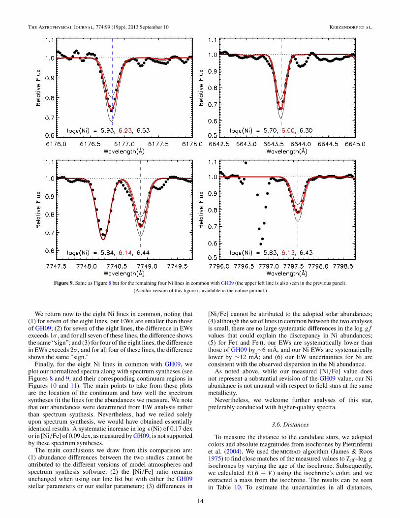
Figure 9. Same as Figure 8 but for the remaining four Ni lines in common with GH09 (the upper left line is also seen in the previous panel).


We return now to the eight Ni lines in common, noting that(1) for seven of the eight lines, our EWs are smaller than thoseof GH09; (2) for seven of the eight lines, the difference in EWsexceeds 1σ , and for all seven of these lines, the difference showsthe same “sign”; and (3) for four of the eight lines, the differencein EWs exceeds 2σ , and for all four of these lines, the differenceshows the same “sign.”

Finally, for the eight Ni lines in common with GH09, weplot our normalized spectra along with spectrum syntheses (seeFigures 8 and 9, and their corresponding continuum regions inFigures 10 and 11). The main points to take from these plotsare the location of the continuum and how well the spectrumsyntheses fit the lines for the abundances we measure. We notethat our abundances were determined from EW analysis ratherthan spectrum synthesis. Nevertheless, had we relied solelyupon spectrum synthesis, we would have obtained essentiallyidentical results. A systematic increase in log ε(Ni) of 0.17 dexor in [Ni/Fe] of 0.09 dex, as measured by GH09, is not supportedby these spectrum syntheses.

The main conclusions we draw from this comparison are:(1) abundance differences between the two studies cannot beattributed to the different versions of model atmospheres andspectrum synthesis software; (2) the [Ni/Fe] ratio remainsunchanged when using our line list but with either the GH09stellar parameters or our stellar parameters; (3) differences in

[Ni/Fe] cannot be attributed to the adopted solar abundances;(4) although the set of lines in common between the two analysesis small, there are no large systematic differences in the log gfvalues that could explain the discrepancy in Ni abundances;(5) for Fe i and Fe ii, our EWs are systematically lower thanthose of GH09 by ∼6 mÅ, and our Ni EWs are systematicallylower by ∼12 mÅ; and (6) our EW uncertainties for Ni areconsistent with the observed dispersion in the Ni abundance.

As noted above, while our measured [Ni/Fe] value doesnot represent a substantial revision of the GH09 value, our Niabundance is not unusual with respect to field stars at the samemetallicity.

Nevertheless, we welcome further analyses of this star,preferably conducted with higher-quality spectra.

3.6. Distances

To measure the distance to the candidate stars, we adoptedcolors and absolute magnitudes from isochrones by Pietrinferniet al. (2004). We used the migrad algorithm (James & Roos1975) to find close matches of the measured values to Teff–log gisochrones by varying the age of the isochrone. Subsequently,we calculated E(B − V ) using the isochrone’s color, and weextracted a mass from the isochrone. The results can be seenin Table 10. To estimate the uncertainties in all distances,

14


Figure 10. Overview of a larger continuum region for the lines measured in Figure 8.

Table 10Distances, Ages, and Masses of Candidate Stars

Tycho Mass σMass Age σAge D σD

(Name) (M/M�) (M/M�) (Gyr) (Gyr) (kpc) (kpc)

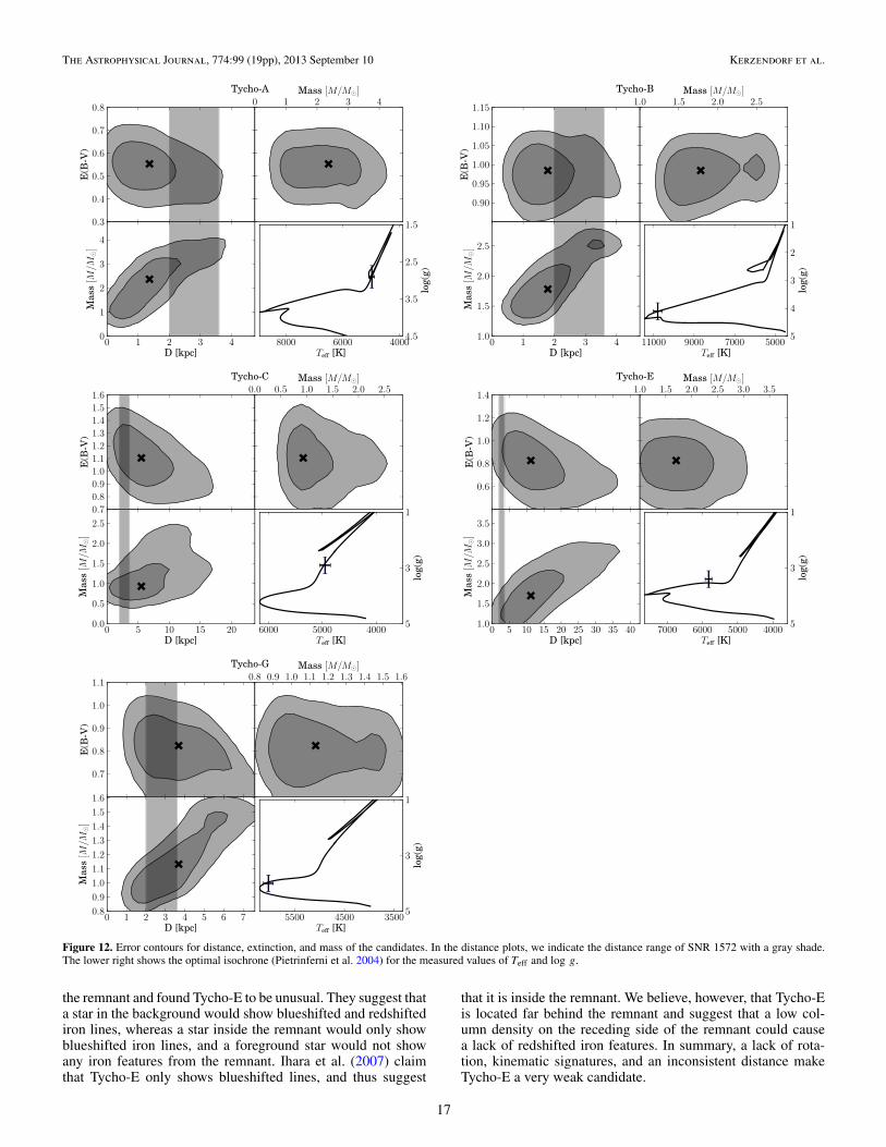
Tycho-A 2.4 0.8 0.7 2.3 1.4 0.8Tycho-B 1.8 0.4 0.8 0.3 1.8 0.8Tycho-C 0.9 0.4 10.0 3.4 5.5 3.5Tycho-E 1.7 0.4 1.4 1.1 11.2 7.5Tycho-G 1.1 0.2 5.7 2.1 3.7 1.5

reddenings, and masses, we employed the Monte Carlo methodwith 10,000 samples of effective temperature, surface gravity,metallicity, B magnitude, and V magnitude (see Figure 12).Errors included in Table 10 are the standard deviations of theMonte Carlo sample. The data show that all stars are compatiblewith the distance of the remnant. This is not unexpected, asthe uncertainties of the measurements in stellar parameters arerelatively large.

4. DISCUSSION

In our sample of six stars, we find no star that showscharacteristics which strongly indicate that it might be the donorstar of SN 1572. On the other hand, it is difficult to absolutelyrule out any particular star, if one is able to invoke improbablepost-explosion evolutionary scenarios.

Tycho-A is a metal-rich giant, and it seems likely to be aforeground star. Its principal redeeming feature as a donor-star candidate is that it is located in the geometric center ofthe remnant and that it has a relatively low surface gravity.Tycho-A shows a very low spatial motion, which is consistentwith a giant-donor-star scenario, although its lack of rotation isin conflict with a donor-star scenario. Taking all measurementsinto account, we regard Tycho-A as a very weak candidate(although a wind accretion scenario might still work).

Tycho-B’s high temperature, position at the center of the rem-nant, high rotational velocity, and unusual chemical abundancemake it the most unusual candidate in the remnant’s center. De-spite the a posteriori unlikely discovery of such a star in the rem-nant’s center, Tycho-B’s high rotational velocity coupled with

15


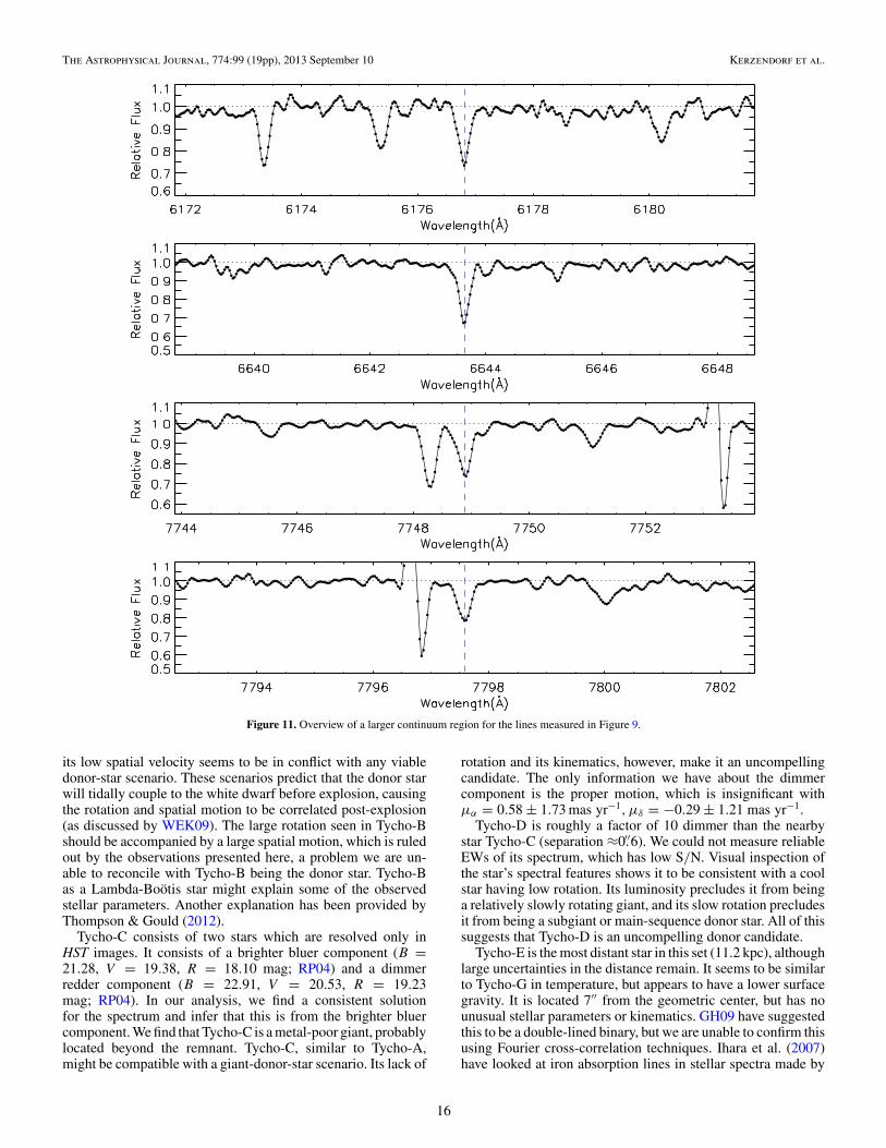
Figure 11. Overview of a larger continuum region for the lines measured in Figure 9.

its low spatial velocity seems to be in conflict with any viabledonor-star scenario. These scenarios predict that the donor starwill tidally couple to the white dwarf before explosion, causingthe rotation and spatial motion to be correlated post-explosion(as discussed by WEK09). The large rotation seen in Tycho-Bshould be accompanied by a large spatial motion, which is ruledout by the observations presented here, a problem we are un-able to reconcile with Tycho-B being the donor star. Tycho-Bas a Lambda-Bootis star might explain some of the observedstellar parameters. Another explanation has been provided byThompson & Gould (2012).

Tycho-C consists of two stars which are resolved only inHST images. It consists of a brighter bluer component (B =21.28, V = 19.38, R = 18.10 mag; RP04) and a dimmerredder component (B = 22.91, V = 20.53, R = 19.23mag; RP04). In our analysis, we find a consistent solutionfor the spectrum and infer that this is from the brighter bluercomponent. We find that Tycho-C is a metal-poor giant, probablylocated beyond the remnant. Tycho-C, similar to Tycho-A,might be compatible with a giant-donor-star scenario. Its lack of

rotation and its kinematics, however, make it an uncompellingcandidate. The only information we have about the dimmercomponent is the proper motion, which is insignificant withμα = 0.58 ± 1.73 mas yr−1, μδ = −0.29 ± 1.21 mas yr−1.

Tycho-D is roughly a factor of 10 dimmer than the nearbystar Tycho-C (separation ≈0.′′6). We could not measure reliableEWs of its spectrum, which has low S/N. Visual inspection ofthe star’s spectral features shows it to be consistent with a coolstar having low rotation. Its luminosity precludes it from beinga relatively slowly rotating giant, and its slow rotation precludesit from being a subgiant or main-sequence donor star. All of thissuggests that Tycho-D is an uncompelling donor candidate.

Tycho-E is the most distant star in this set (11.2 kpc), althoughlarge uncertainties in the distance remain. It seems to be similarto Tycho-G in temperature, but appears to have a lower surfacegravity. It is located 7′′ from the geometric center, but has nounusual stellar parameters or kinematics. GH09 have suggestedthis to be a double-lined binary, but we are unable to confirm thisusing Fourier cross-correlation techniques. Ihara et al. (2007)have looked at iron absorption lines in stellar spectra made by

16


0.3

0.4

0.5

0.6

0.7

0.8

E(B

-V)

0 1 2 3 4Mass [M/M ]

0 1 2 3 4D [kpc]

0

1

2

3

4

Mas

s[M

/M]

400060008000Teff [K]

1.5

2.5

3.5

4.5

log(

g)

Tycho-A

0.90

0.95

1.00

1.05

1.10

1.15

E(B

-V)

1.0 1.5 2.0 2.5Mass [M/M ]

0 1 2 3 4D [kpc]

1.0

1.5

2.0

2.5

Mas

s[M

/M]

50007000900011000Teff [K]

1

2

3

4

5

log(

g)

Tycho-B

0.7

0.8

0.9

1.0

1.1

1.2

1.3

1.4

1.5

1.6

E(B

-V)

0.0 0.5 1.0 1.5 2.0 2.5Mass [M/M ]

0 5 10 15 20D [kpc]

0.0

0.5

1.0

1.5

2.0

2.5

Mas

s[M

/M]

400050006000Teff [K]

1

3

5

log(

g)

Tycho-C

0.6

0.8

1.0

1.2

1.4

E(B

-V)

1.0 1.5 2.0 2.5 3.0 3.5Mass [M/M ]

0 5 10 15 20 25 30 35 40D [kpc]

1.0

1.5

2.0

2.5

3.0

3.5

Mas

s[M

/M]

4000500060007000Teff [K]

1

3

5

log(

g)

Tycho-E

0.7

0.8

0.9

1.0

1.1

E(B

-V)

0.8 0.9 1.0 1.1 1.2 1.3 1.4 1.5 1.6Mass [M/M ]

0 1 2 3 4 5 6 7D [kpc]

0.8

0.9

1.0

1.1

1.2

1.3

1.4

1.5

1.6

Mas

s[M

/M]

350045005500Teff [K]

1

3

5

log(

g)

Tycho-G

Figure 12. Error contours for distance, extinction, and mass of the candidates. In the distance plots, we indicate the distance range of SNR 1572 with a gray shade.The lower right shows the optimal isochrone (Pietrinferni et al. 2004) for the measured values of Teff and log g.

the remnant and found Tycho-E to be unusual. They suggest thata star in the background would show blueshifted and redshiftediron lines, whereas a star inside the remnant would only showblueshifted iron lines, and a foreground star would not showany iron features from the remnant. Ihara et al. (2007) claimthat Tycho-E only shows blueshifted lines, and thus suggest

that it is inside the remnant. We believe, however, that Tycho-Eis located far behind the remnant and suggest that a low col-umn density on the receding side of the remnant could causea lack of redshifted iron features. In summary, a lack of rota-tion, kinematic signatures, and an inconsistent distance makeTycho-E a very weak candidate.

17


Tycho-G is located 30′′ from the X-ray center, making itthe most remote object from the center in this work (in theplane of the sky; for comparison a distance of 32.′′6 cor-responds to 1000 km s−1 over 433 yr at the distance of2.8 kpc). This work confirms the radial velocity measuredby GH09 and WEK09. Figure 2 shows the expected distribu-tion of radial velocities from the Besancon model of Galac-tic dynamics. Tycho-G lies well within the expected rangeof radial velocity for stars with its stellar parameters anddistance.

In addition, this work has analyzed the proper motion ofstars around the center of SN 1572. Figure 1 shows Tycho-Gto be a 2σ outlier, which implies that there should be aboutsix stars in the HST sample sharing similar proper-motionfeatures as Tycho-G; thus, its proper motion is by no meansa unique trait. In particular, stars in the thick disk have motionsentirely consistent with that of Tycho-G (see contours inFigure 1, and Figure 10 in GH09). Finally, the HST proper-motion measurements are challenging, and it is conceivable thatthere are systematic errors in our proper-motion measurementswhich are larger than our reported statistical errors. Sucherrors would tend to increase the chance of larger-than-actualproper-motion measurements. Taken in total, while Tycho-Gmay have an unusual proper motion, the significance of thismotion, even if current measurements are exactly correct, is notexceptional.

As described, the kinematic features of a donor star mighteasily be lost in the kinematic noise of the Galaxy. WEK09recommend using post-explosion stellar rotation as an additionalpossible feature for a donor star. This work suggests thatTycho-G has a rotation below the instrumental profile of6 km s−1, much less than expected for a donor star (for anestimate, see Kerzendorf et al. 2009). Recently, Pan et al. (2012a,2012b) suggested that taking only tidal coupling into accountcould overestimate the rotation. However, all of their models(see Table 3 of Pan et al. 2012a) having a relatively low rotationrate are too luminous and too large to be consistent with Tycho-G. In fact, none of their calculated models can satisfy theconstraints of the measured log g and the upper limit on vrotsimultaneously.

We find Tycho-G to be a subgiant/main-sequence star withroughly solar temperature and metallicity. GH09 measure anickel enhancement, which they believe to originate in thecontamination from the ejecta. We have conducted a detailedcomparison with GH09’s measurement in Section 3.5 and do notfind Tycho-G to be an outlier as suggested by GH09, but ratherconsistent with other stars of similar metallicity. In addition, ourLi measurement is in agreement with that of GH09 (see Table 6).In contrast to the GH09 interpretation, this Li abundance isconsistent with that of stars of similar parameters (Baumannet al. 2010). Finally, we have measured the distance to Tycho-G,showing it to be consistent with a background star. In addition,the radial-velocity signature matches that of background stars(see Figure 2).

In summary, while Tycho-G may have unusual kinematics asindicated by its proper motion, the significance of this motionis not compelling when compared to a large sample of similarstars in the direction of the Tycho remnant. Furthermore, sucha kinematic signature, if it were related to the binary orbitalvelocity, might predict rotation for Tycho-G which we do notobserve (modulo the caveats from WEK09 and Pan et al. 2012b).All of the above evidence makes Tycho-G consistent with abackground thick-disk interloper.

5. CONCLUSION

This work did not detect an unambiguously identifiabledonor-star candidate to Tycho’s SN 1572. Although Tycho-Bshows some unusual features, there currently remains no con-vincing explanation for all of its parameters which can be at-tributed to the donor-star scenario. We believe that our resultsprovide evidence that the Tycho SNR does not have a main-sequence, subgiant, or red giant donor star. Some other possi-bilities remain. In the spin-down scenario, the companion starcan become a helium white dwarf from a red giant donor, or avery low-mass main-sequence star from a more massive main-sequence star. Such a compact companion can escape detection(Di Stefano et al. 2011; Justham 2011; Hachisu et al. 2012a,2012b). Another scenario is a helium donor, such as the so-called sub-Chandrasekhar mass explosions discussed by Livne& Arnett (1995) and Sim et al. (2010). These progenitor sys-tems might leave a very faint and fast-moving helium star, or noremnant at all (R. Pakmor 2012, private communication). Such aprogenitor would probably evade detection and would likely notleave traces, such as circumstellar interaction with the remnantor early light-curve anomalies (Kasen 2010). Deep multi-epochwide-field optical images should catch any such star speedingaway from the remnant’s center, but observations of this kindhave not yet been taken. Finally, a double-degenerate progen-itor, in most cases, does not leave a compact remnant, and isconsistent with our finding no donor star in SNR 1572.

SN 1006 and SN 1604 (Kepler’s SN) are two other SNIa remnants in the Milky Way. SN 1006 is far from theGalactic plane and shows no signs of circumstellar interaction.Kerzendorf et al. (2012) have studied this remnant and havenot found any unusual star that can be explained with a donor-star scenario (consistent with this work). SNR 1604, while farfrom the Galactic plane, shows circumstellar interaction with itsremnant and has all the indications of what might be expectedfrom an SD-scenario with an asymptotic giant branch donor(Chiotellis et al. 2012). Observations of these remnants willbetter establish if there is a continued pattern to the unusualstars in SN Ia remnant centers, or whether the lack of viabledonor stars persists in multiple systems.

B. P. Schmidt and W. E. Kerzendorf were supported bySchmidt’s ARC Laureate Fellowship (FL0992131). A. Gal-Yam acknowledges support by the Israeli Science Foundation.A. V. Filippenko is grateful for the support of the ChristopherR. Redlich Fund, the TABASGO Foundation, and NSF grantsAST-0908886 and AST-1211916; funding was also providedby NASA grants GO-10098, GO-12469, and AR-12623 fromthe Space Telescope Science Institute, which is operated byAURA, Inc., under NASA contract NAS 5-26555. R. J. Foleywas supported by a Clay Fellowship.

Some of the data presented herein were obtained at the W. M.Keck Observatory, which is operated as a scientific partnershipamong the California Institute of Technology, the University ofCalifornia, and NASA; the observatory was made possible bythe generous financial support of the W. M. Keck Foundation.

We thank Christopher Onken and Jorge Melendez for helpfuladvice on the HIRES data reduction. We acknowledge usefuldiscussions about differential rotation with Amanda Karakas,and we also thank Peter Wood for advising us on stellar evolutionmatters. Rudiger Pakmor provided information on helium-starmergers. We thank Martin Asplund for providing us with LiNLTE corrections.

18


REFERENCES

Anderson, J., & King, I. R. 2006, PSFs, Photometry, and Astronomy for theACS/WFC, Tech. Rep.

Asplund, M., Grevesse, N., Sauval, A. J., & Scott, P. 2009, ARA&A, 47, 481Badenes, C., Borkowski, K. J., Hughes, J. P., Hwang, U., & Bravo, E. 2006, ApJ,

645, 1373Baumann, P., Ramırez, I., Melendez, J., Asplund, M., & Lind, K. 2010, A&A,

519, A87Beals, C. S., & Blanchet, G. H. 1937, PASP, 49, 224Bensby, T., Feltzing, S., Lundstrom, I., & Ilyin, I. 2005, A&A, 433, 185Bessell, M. S. 2007, PASP, 119, 605Bianco, F. B., Howell, D. A., Sullivan, M., et al. 2011, ApJ, 741, 20Biemont, E., Baudoux, M., Kurucz, R. L., Ansbacher, W., & Pinnington, E. H.

1991, A&A, 249, 539Blackwell, D. E., Booth, A. J., Haddock, D. J., Petford, A. D., & Leggett, S. K.

1986, MNRAS, 220, 549Blackwell, D. E., Ibbetson, P. A., Petford, A. D., & Shallis, M. J. 1979a,

MNRAS, 186, 633Blackwell, D. E., Lynas-Gray, A. E., & Smith, G. 1995, A&A, 296, 217Blackwell, D. E., Petford, A. D., & Shallis, M. J. 1979b, MNRAS, 186, 657Blackwell, D. E., Petford, A. D., Shallis, M. J., & Simmons, G. J. 1980, MNRAS,

191, 445Bloom, J. S., Kasen, D., Shen, K. J., et al. 2012, ApJL, 744, L17Brown, P. J., Dawson, K. S., de Pasquale, M., et al. 2012, ApJ, 753, 22Castelli, F., & Kurucz, R. L. 2003, in IAU Symp. 210, Modelling of Stellar

Atmospheres, ed. N. Piskunov, W. W. Weiss, & D. F. Gray (San Francisco,CA: ASP), 20

Castelli, F., & Kurucz, R. L. 2004, arXiv Astrophysics e-printsCayrel, R. 1988, in IAU Symp. 132, The Impact of Very High S/N Spectroscopy

on Stellar Physics, ed. G. Cayrel de Strobel & M. Spite (Dordrecht: Kluwer),345

Chiotellis, A., Schure, K. M., & Vink, J. 2012, A&A, 537, A139Chomiuk, L., Soderberg, A. M., Moe, M., et al. 2012, ApJ, 750, 164Dan, M., Rosswog, S., Guillochon, J., & Ramirez-Ruiz, E. 2011, ApJ, 737, 89Di Stefano, R., Voss, R., & Claeys, J. S. W. 2011, ApJL, 738, L1Filippenko, A. V. 1997, ARA&A, 35, 309Fink, M., Ropke, F. K., Hillebrandt, W., et al. 2010, A&A, 514, A53Foley, R. J., Papenkova, M. S., Swift, B. J., et al. 2003, PASP, 115, 1220Foley, R. J., Simon, J. D., Burns, C. R., et al. 2012, ApJ, 752, 101Ganeshalingam, M., Li, W., & Filippenko, A. V. 2011, MNRAS, 416, 2607Gonzalez Hernandez, J. I., Ruiz-Lapuente, P., Filippenko, A. V., et al. 2009, ApJ,

691, 1Hachisu, I., Kato, M., & Nomoto, K. 2012a, ApJL, 756, L4Hachisu, I., Kato, M., Saio, H., & Nomoto, K. 2012b, ApJ, 744, 69Han, Z. 2008, ApJL, 677, L109Hayden, B. T., Garnavich, P. M., Kasen, D., et al. 2010, ApJ, 722, 1691Heiter, U., Kupka, F., van’t Veer-Menneret, C., et al. 2002, A&A, 392, 619Herbig, G. H. 1966, ZA, 64, 512Herbig, G. H. 1967, in IAU Symp. 31, Radio Astronomy and the Galactic

System, ed. H. van Woerden (London: Academic), 85Herbig, G. H. 1975, ApJ, 196, 129Herbig, G. H. 1995, ARA&A, 33, 19Hibbins, R. E., Miles, J. R., Sarre, P. J., & Herbig, G. H. 1994, in The Diffuse

Interstellar Bands, ed. A. G. G. M. Tielens, 31Hinkle, K., Wallace, L., Harmer, D., Ayres, T., & Valenti, J. 2000, in the 24th

Meeting of the IAU, Joint Discussion, Vol. 1, High Resolution IR, Visible,and UV Spectroscopy of the Sun and Arcturus, ed. H. Rickman (Manchester:IAU)

Horesh, A., Kulkarni, S. R., Fox, D. B., et al. 2012, ApJ, 746, 21Horne, K. 1986, PASP, 98, 609

Hughes, J. P. 2000, ApJL, 545, L53Ihara, Y., Ozaki, J., Doi, M., et al. 2007, PASJ, 59, 811James, F., & Roos, M. 1975, CoPhC, 10, 343Jeffery, C. S., Woolf, V. M., & Pollacco, D. L. 2001, A&A, 376, 497Jenniskens, P., & Desert, F. 1994, A&AS, 106, 39Justham, S. 2011, ApJL, 730, L34Kasen, D. 2010, ApJ, 708, 1025Kerzendorf, W. E., Schmidt, B. P., Asplund, M., et al. 2009, ApJ, 701, 1665Kerzendorf, W. E., Schmidt, B. P., Laird, J. B., Posiadlowski, P., & Bessell,

M. S. 2012, ApJ, 759, 7Krause, O., Tanaka, M., Usuda, T., et al. 2008, Natur, 456, 617Kupka, F. G., Ryabchikova, T. A., Piskunov, N. E., Stempels, H. C., & Weiss,

W. W. 2000, BaltA, 9, 590Kurucz, R., & Bell, B. 1995, Atomic Line Data Kurucz CD-ROM No. 23

(Cambridge, MA: Smithsonian Astrophysical Observatory), 23Leonard, D. C. 2007, ApJ, 670, 1275Li, W., Bloom, J. S., Podsiadlowski, P., et al. 2011, Natur, 480, 348Lind, K., Asplund, M., & Barklem, P. S. 2009, A&A, 503, 541Livne, E., & Arnett, D. 1995, ApJ, 452, 62Luck, R. E., & Heiter, U. 2007, AJ, 133, 2464Matheson, T., Filippenko, A. V., Ho, L. C., Barth, A. J., & Leonard, D. C.

2000, AJ, 120, 1499Mennekens, N., Vanbeveren, D., De Greve, J. P., & De Donder, E. 2010, A&A,

515, A89Munari, U., Sordo, R., Castelli, F., & Zwitter, T. 2005, A&A, 442, 1127Nugent, P. E., Sullivan, M., Cenko, S. B., et al. 2011, Natur, 480, 344Oke, J. B., Cohen, J. G., Carr, M., et al. 1995, PASP, 107, 375Pakmor, R., Kromer, M., Ropke, F. K., et al. 2010, Natur, 463, 61Pan, K.-C., Ricker, P. M., & Taam, R. E. 2012a, ApJ, 760, 21Pan, K.-C., Ricker, P. M., & Taam, R. E. 2012b, ApJ, 750, 151Patat, F., Chandra, P., Chevalier, R., et al. 2007, Sci, 317, 924Pietrinferni, A., Cassisi, S., Salaris, M., & Castelli, F. 2004, ApJ, 612, 168Ramırez, S. V., & Cohen, J. G. 2002, AJ, 123, 3277Reddy, B. E., Tomkin, J., Lambert, D. L., & Allende Prieto, C. 2003, MNRAS,

340, 304Rest, A., Welch, D. L., Suntzeff, N. B., et al. 2008, ApJL, 681, L81Reynoso, E. M., Moffett, D. A., Goss, W. M., et al. 1997, ApJ, 491, 816Robin, A. C., Reyle, C., Derriere, S., & Picaud, S. 2003, A&A, 409, 523Ruiter, A. J., Belczynski, K., & Fryer, C. 2009, ApJ, 699, 2026Ruiz-Lapuente, P. 2004, ApJ, 612, 357Ruiz-Lapuente, P., Comeron, F., Mendez, J., et al. 2004, Natur, 431, 1069Saio, H., & Nomoto, K. 1985, A&A, 150, L21Sim, S. A., Ropke, F. K., Hillebrandt, W., et al. 2010, ApJL, 714, L52Simon, J. D., Gal-Yam, A., Gnat, O., et al. 2009, ApJ, 702, 1157Sneden, C. 1973, ApJ, 184, 839Sobeck, J. S., Kraft, R. P., Sneden, C., et al. 2011, AJ, 141, 175Stefanik, R. P., Latham, D. W., & Torres, G. 1999, in ASP Conf. Ser. 185, IAU

Colloq. 170, Precise Stellar Radial Velocities, ed. J. B. Hearnshaw & C. D.Scarfe (San Francisco, CA: ASP), 354

Sternberg, A., Gal-Yam, A., Simon, J. D., et al. 2011, Sci, 333, 856Stetson, P. B., & Pancino, E. 2008, PASP, 120, 1332Thompson, T. A., & Gould, A. 2012, arXiv:1210.6050Tonry, J., & Davis, M. 1979, AJ, 84, 1511Tucker, B. E. 2011, Ap&SS, 335, 223Vogt, S. S., Allen, S. L., Bigelow, B. C., et al. 1994, Proc. SPIE, 2198, 362Warren, J. S., Hughes, J. P., Badenes, C., et al. 2005, ApJ, 634, 376Wilson, R. 1958, ApJ, 128, 57Winkler, P. F., Gupta, G., & Long, K. S. 2003, ApJ, 585, 324Yaron, O., & Gal-Yam, A. 2012, PASP, 124, 668Yong, D., Lambert, D. L., Paulson, D. B., & Carney, B. W. 2008, ApJ, 673, 854Yu, S., & Jeffery, C. S. 2010, A&A, 521, A85

19

http://dx.doi.org/10.1146/annurev.astro.46.060407.145222

http://adsabs.harvard.edu/abs/2009ARA&A..47..481A

http://adsabs.harvard.edu/abs/2009ARA&A..47..481A

http://dx.doi.org/10.1086/504399

http://adsabs.harvard.edu/abs/2006ApJ...645.1373B

http://adsabs.harvard.edu/abs/2006ApJ...645.1373B

http://dx.doi.org/10.1051/0004-6361/201015137

http://adsabs.harvard.edu/abs/2010A&A...519A..87B

http://adsabs.harvard.edu/abs/2010A&A...519A..87B

http://dx.doi.org/10.1086/124828

http://adsabs.harvard.edu/abs/1937PASP...49..224B

http://adsabs.harvard.edu/abs/1937PASP...49..224B

http://dx.doi.org/10.1051/0004-6361:20040332

http://adsabs.harvard.edu/abs/2005A&A...433..185B


http://dx.doi.org/10.1086/519981

http://adsabs.harvard.edu/abs/2007PASP..119..605B

http://adsabs.harvard.edu/abs/2007PASP..119..605B

http://dx.doi.org/10.1088/0004-637X/741/1/20

http://adsabs.harvard.edu/abs/2011ApJ...741...20B




http://adsabs.harvard.edu/abs/1986MNRAS.220..549B










http://dx.doi.org/10.1088/2041-8205/744/2/L17

http://adsabs.harvard.edu/abs/2012ApJ...744L..17B

http://adsabs.harvard.edu/abs/2012ApJ...744L..17B

http://dx.doi.org/10.1088/0004-637X/753/1/22



http://adsabs.harvard.edu/abs/1988IAUS..132..345C

http://dx.doi.org/10.1051/0004-6361/201014754

http://adsabs.harvard.edu/abs/2012A&A...537A.139C

http://adsabs.harvard.edu/abs/2012A&A...537A.139C

http://dx.doi.org/10.1088/0004-637X/750/2/164

http://adsabs.harvard.edu/abs/2012ApJ...750..164C

http://adsabs.harvard.edu/abs/2012ApJ...750..164C

http://dx.doi.org/10.1088/0004-637X/737/2/89

http://adsabs.harvard.edu/abs/2011ApJ...737...89D

http://adsabs.harvard.edu/abs/2011ApJ...737...89D

http://dx.doi.org/10.1088/2041-8205/738/1/L1

http://adsabs.harvard.edu/abs/2011ApJ...738L...1D

http://adsabs.harvard.edu/abs/2011ApJ...738L...1D

http://dx.doi.org/10.1146/annurev.astro.35.1.309

http://adsabs.harvard.edu/abs/1997ARA&A..35..309F

http://adsabs.harvard.edu/abs/1997ARA&A..35..309F

http://dx.doi.org/10.1051/0004-6361/200913892

http://adsabs.harvard.edu/abs/2010A&A...514A..53F

http://adsabs.harvard.edu/abs/2010A&A...514A..53F

http://dx.doi.org/10.1086/378242

http://adsabs.harvard.edu/abs/2003PASP..115.1220F

http://adsabs.harvard.edu/abs/2003PASP..115.1220F

http://dx.doi.org/10.1088/0004-637X/752/2/101

http://adsabs.harvard.edu/abs/2012ApJ...752..101F

http://adsabs.harvard.edu/abs/2012ApJ...752..101F

http://dx.doi.org/10.1111/j.1365-2966.2011.19213.x

http://adsabs.harvard.edu/abs/2011MNRAS.416.2607G

http://adsabs.harvard.edu/abs/2011MNRAS.416.2607G

http://dx.doi.org/10.1088/0004-637X/691/1/1

http://adsabs.harvard.edu/abs/2009ApJ...691....1G

http://adsabs.harvard.edu/abs/2009ApJ...691....1G

http://dx.doi.org/10.1088/2041-8205/756/1/L4

http://adsabs.harvard.edu/abs/2012ApJ...756L...4H

http://adsabs.harvard.edu/abs/2012ApJ...756L...4H

http://dx.doi.org/10.1088/0004-637X/744/1/69

http://adsabs.harvard.edu/abs/2012ApJ...744...69H


http://dx.doi.org/10.1086/588191

http://adsabs.harvard.edu/abs/2008ApJ...677L.109H

http://adsabs.harvard.edu/abs/2008ApJ...677L.109H

http://dx.doi.org/10.1088/0004-637X/722/2/1691

http://adsabs.harvard.edu/abs/2010ApJ...722.1691H

http://adsabs.harvard.edu/abs/2010ApJ...722.1691H

http://dx.doi.org/10.1051/0004-6361:20020788

http://adsabs.harvard.edu/abs/2002A&A...392..619H

http://adsabs.harvard.edu/abs/2002A&A...392..619H

http://adsabs.harvard.edu/abs/1966ZA.....64..512H

http://adsabs.harvard.edu/abs/1966ZA.....64..512H

http://adsabs.harvard.edu/abs/1967IAUS...31...85H

http://dx.doi.org/10.1086/153400

http://adsabs.harvard.edu/abs/1975ApJ...196..129H

http://adsabs.harvard.edu/abs/1975ApJ...196..129H

http://dx.doi.org/10.1146/annurev.aa.33.090195.000315

http://adsabs.harvard.edu/abs/1995ARA&A..33...19H

http://adsabs.harvard.edu/abs/1995ARA&A..33...19H

http://adsabs.harvard.edu/abs/1994dib..nasa...31H

http://dx.doi.org/10.1088/0004-637X/746/1/21



http://dx.doi.org/10.1086/131801

http://adsabs.harvard.edu/abs/1986PASP...98..609H

http://adsabs.harvard.edu/abs/1986PASP...98..609H

http://dx.doi.org/10.1086/317337

http://adsabs.harvard.edu/abs/2000ApJ...545L..53H

http://adsabs.harvard.edu/abs/2000ApJ...545L..53H

http://adsabs.harvard.edu/abs/2007PASJ...59..811I

http://adsabs.harvard.edu/abs/2007PASJ...59..811I

http://adsabs.harvard.edu/abs/1975CoPhC..10..343J

http://adsabs.harvard.edu/abs/1975CoPhC..10..343J

http://dx.doi.org/10.1051/0004-6361:20010954

http://adsabs.harvard.edu/abs/2001A&A...376..497J

http://adsabs.harvard.edu/abs/2001A&A...376..497J

http://adsabs.harvard.edu/abs/1994A&AS..106...39J

http://adsabs.harvard.edu/abs/1994A&AS..106...39J

http://dx.doi.org/10.1088/2041-8205/730/2/L34

http://adsabs.harvard.edu/abs/2011ApJ...730L..34J

http://adsabs.harvard.edu/abs/2011ApJ...730L..34J

http://dx.doi.org/10.1088/0004-637X/708/2/1025

http://adsabs.harvard.edu/abs/2010ApJ...708.1025K


http://dx.doi.org/10.1088/0004-637X/701/2/1665



http://dx.doi.org/10.1088/0004-637X/759/1/7

http://adsabs.harvard.edu/abs/2012ApJ...759....7K

http://adsabs.harvard.edu/abs/2012ApJ...759....7K

http://dx.doi.org/10.1038/nature07608

http://adsabs.harvard.edu/abs/2008Natur.456..617K

http://adsabs.harvard.edu/abs/2008Natur.456..617K

http://adsabs.harvard.edu/abs/2000BaltA...9..590K

http://adsabs.harvard.edu/abs/2000BaltA...9..590K

http://adsabs.harvard.edu/abs/1995all..book.....K

http://dx.doi.org/10.1086/522367

http://adsabs.harvard.edu/abs/2007ApJ...670.1275L

http://adsabs.harvard.edu/abs/2007ApJ...670.1275L


http://adsabs.harvard.edu/abs/2011Natur.480..348L

http://adsabs.harvard.edu/abs/2011Natur.480..348L

http://dx.doi.org/10.1051/0004-6361/200912221

http://adsabs.harvard.edu/abs/2009A&A...503..541L

http://adsabs.harvard.edu/abs/2009A&A...503..541L

http://dx.doi.org/10.1086/176279

http://adsabs.harvard.edu/abs/1995ApJ...452...62L

http://adsabs.harvard.edu/abs/1995ApJ...452...62L

http://dx.doi.org/10.1086/513194

http://adsabs.harvard.edu/abs/2007AJ....133.2464L

http://adsabs.harvard.edu/abs/2007AJ....133.2464L

http://dx.doi.org/10.1086/301519

http://adsabs.harvard.edu/abs/2000AJ....120.1499M

http://adsabs.harvard.edu/abs/2000AJ....120.1499M

http://dx.doi.org/10.1051/0004-6361/201014115

http://adsabs.harvard.edu/abs/2010A&A...515A..89M

http://adsabs.harvard.edu/abs/2010A&A...515A..89M

http://dx.doi.org/10.1051/0004-6361:20042490

http://adsabs.harvard.edu/abs/2005A&A...442.1127M

http://adsabs.harvard.edu/abs/2005A&A...442.1127M


http://adsabs.harvard.edu/abs/2011Natur.480..344N

http://adsabs.harvard.edu/abs/2011Natur.480..344N

http://dx.doi.org/10.1086/133562

http://adsabs.harvard.edu/abs/1995PASP..107..375O

http://adsabs.harvard.edu/abs/1995PASP..107..375O


http://adsabs.harvard.edu/abs/2010Natur.463...61P

http://adsabs.harvard.edu/abs/2010Natur.463...61P

http://dx.doi.org/10.1088/0004-637X/760/1/21

http://adsabs.harvard.edu/abs/2012ApJ...760...21P

http://adsabs.harvard.edu/abs/2012ApJ...760...21P

http://dx.doi.org/10.1088/0004-637X/750/2/151

http://adsabs.harvard.edu/abs/2012ApJ...750..151P


http://dx.doi.org/10.1126/science.1143005

http://adsabs.harvard.edu/abs/2007Sci...317..924P

http://adsabs.harvard.edu/abs/2007Sci...317..924P

http://dx.doi.org/10.1086/422498



http://dx.doi.org/10.1086/340354

http://adsabs.harvard.edu/abs/2002AJ....123.3277R

http://adsabs.harvard.edu/abs/2002AJ....123.3277R

http://dx.doi.org/10.1046/j.1365-8711.2003.06305.x

http://adsabs.harvard.edu/abs/2003MNRAS.340..304R

http://adsabs.harvard.edu/abs/2003MNRAS.340..304R

http://dx.doi.org/10.1086/590427

http://adsabs.harvard.edu/abs/2008ApJ...681L..81R

http://adsabs.harvard.edu/abs/2008ApJ...681L..81R

http://dx.doi.org/10.1086/304997

http://adsabs.harvard.edu/abs/1997ApJ...491..816R


http://dx.doi.org/10.1051/0004-6361:20031117

http://adsabs.harvard.edu/abs/2003A&A...409..523R

http://adsabs.harvard.edu/abs/2003A&A...409..523R

http://dx.doi.org/10.1088/0004-637X/699/2/2026

http://adsabs.harvard.edu/abs/2009ApJ...699.2026R

http://adsabs.harvard.edu/abs/2009ApJ...699.2026R

http://dx.doi.org/10.1086/422419




http://adsabs.harvard.edu/abs/2004Natur.431.1069R

http://adsabs.harvard.edu/abs/2004Natur.431.1069R

http://adsabs.harvard.edu/abs/1985A&A...150L..21S

http://adsabs.harvard.edu/abs/1985A&A...150L..21S

http://dx.doi.org/10.1088/2041-8205/714/1/L52

http://adsabs.harvard.edu/abs/2010ApJ...714L..52S

http://adsabs.harvard.edu/abs/2010ApJ...714L..52S

http://dx.doi.org/10.1088/0004-637X/702/2/1157

http://adsabs.harvard.edu/abs/2009ApJ...702.1157S

http://adsabs.harvard.edu/abs/2009ApJ...702.1157S

http://dx.doi.org/10.1086/152374

http://adsabs.harvard.edu/abs/1973ApJ...184..839S

http://adsabs.harvard.edu/abs/1973ApJ...184..839S

http://dx.doi.org/10.1088/0004-6256/141/6/175

http://adsabs.harvard.edu/abs/2011AJ....141..175S

http://adsabs.harvard.edu/abs/2011AJ....141..175S

http://adsabs.harvard.edu/abs/1999IAUCo.170..354S

http://dx.doi.org/10.1126/science.1203836

http://adsabs.harvard.edu/abs/2011Sci...333..856S

http://adsabs.harvard.edu/abs/2011Sci...333..856S

http://dx.doi.org/10.1086/596126

http://adsabs.harvard.edu/abs/2008PASP..120.1332S

http://adsabs.harvard.edu/abs/2008PASP..120.1332S

http://www.arxiv.org/abs/1210.6050

http://dx.doi.org/10.1086/112569

http://adsabs.harvard.edu/abs/1979AJ.....84.1511T

http://adsabs.harvard.edu/abs/1979AJ.....84.1511T

http://dx.doi.org/10.1007/s10509-011-0615-z

http://adsabs.harvard.edu/abs/2011Ap&SS.335..223T

http://adsabs.harvard.edu/abs/2011Ap&SS.335..223T

http://dx.doi.org/10.1117/12.176725

http://adsabs.harvard.edu/abs/1994SPIE.2198..362V

http://adsabs.harvard.edu/abs/1994SPIE.2198..362V

http://dx.doi.org/10.1086/496941

http://adsabs.harvard.edu/abs/2005ApJ...634..376W


http://dx.doi.org/10.1086/146515

http://adsabs.harvard.edu/abs/1958ApJ...128...57W

http://adsabs.harvard.edu/abs/1958ApJ...128...57W

http://dx.doi.org/10.1086/345985



http://dx.doi.org/10.1086/666656

http://adsabs.harvard.edu/abs/2012PASP..124..668Y

http://adsabs.harvard.edu/abs/2012PASP..124..668Y

http://dx.doi.org/10.1086/524376

http://adsabs.harvard.edu/abs/2008ApJ...673..854Y

http://adsabs.harvard.edu/abs/2008ApJ...673..854Y

http://dx.doi.org/10.1051/0004-6361/201014827

http://adsabs.harvard.edu/abs/2010A&A...521A..85Y

http://adsabs.harvard.edu/abs/2010A&A...521A..85Y

Documents

A HIGH-RESOLUTION SPECTROSCOPIC SEARCH FOR THE …