1

UNIT-5

Searching: List Searches- Sequential Search- Variations on Sequential Searches- Binary Search- Analyzing

Search Algorithm- Hashed List Searches- Basic Concepts- Hashing Methods- Collision Resolutions- Open Addressing- Linked List Collision Resolution- Bucket Hashing.

5.1 List Searches

Searching is the process used to find the location of a target among a list of objects.

The two basic searches for arrays are the sequential search and the binary search. a) The sequential search can be used to locate an item in any array. b) The binary search, on the other hand, requires an ordered list.

5.2 Sequential search

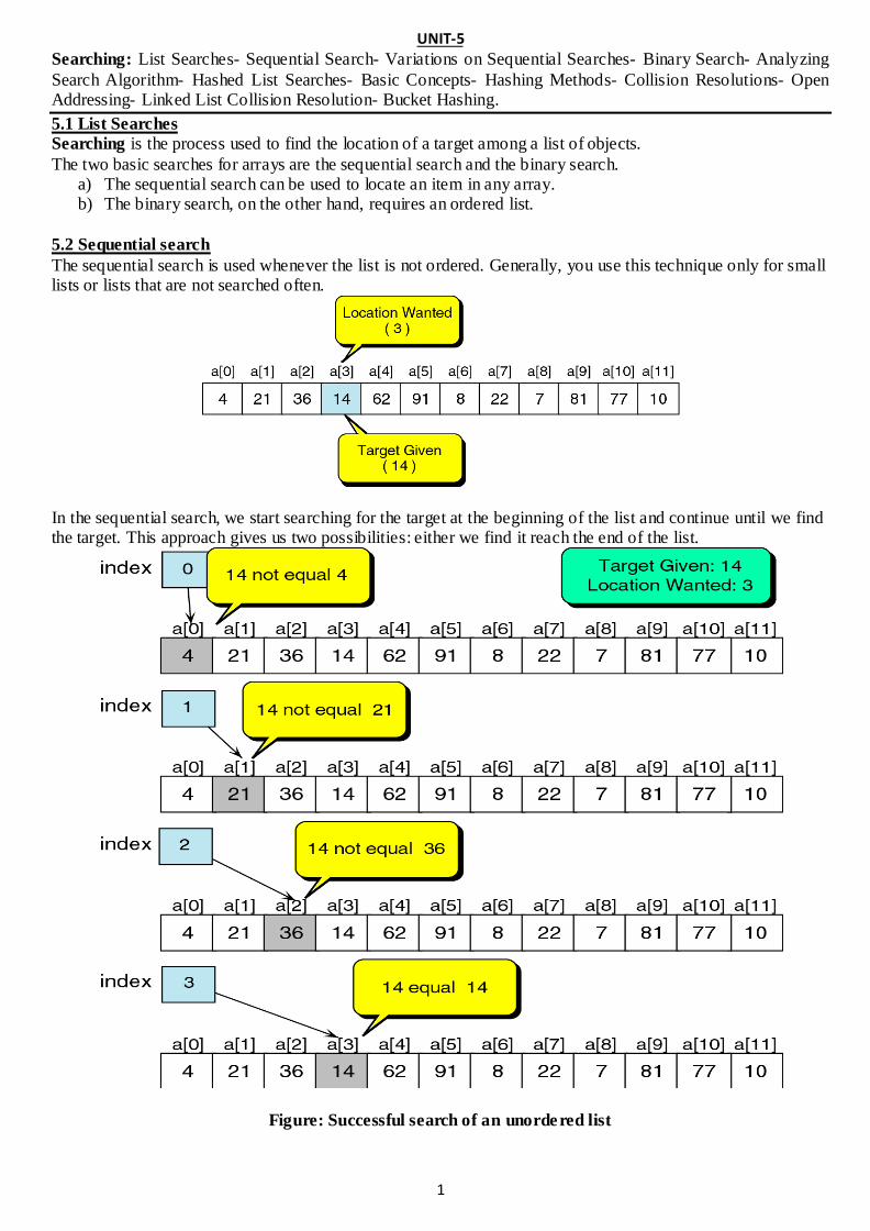
The sequential search is used whenever the list is not ordered. Generally, you use this technique only for small lists or lists that are not searched often.

In the sequential search, we start searching for the target at the beginning of the list and continue until we find the target. This approach gives us two possibilities: either we find it reach the end of the list.

Figure: Successful search of an unordered list

2

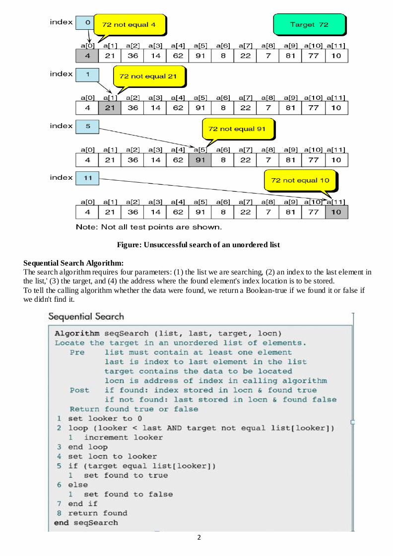
Figure: Unsuccessful search of an unordered list

Sequential Search Algorithm:

The search algorithm requires four parameters: (1) the list we are searching, (2) an index to the last element in the list,' (3) the target, and (4) the address where the found element's index location is to be stored.

To tell the calling algorithm whether the data were found, we return a Boolean-true if we found it or false if we didn't find it.

3

5.3 Variations on Sequential Searches

Three useful variations on the sequential search algorithm are: (I) the sentinel search, (2) the probability

search, and (3) the ordered list search.

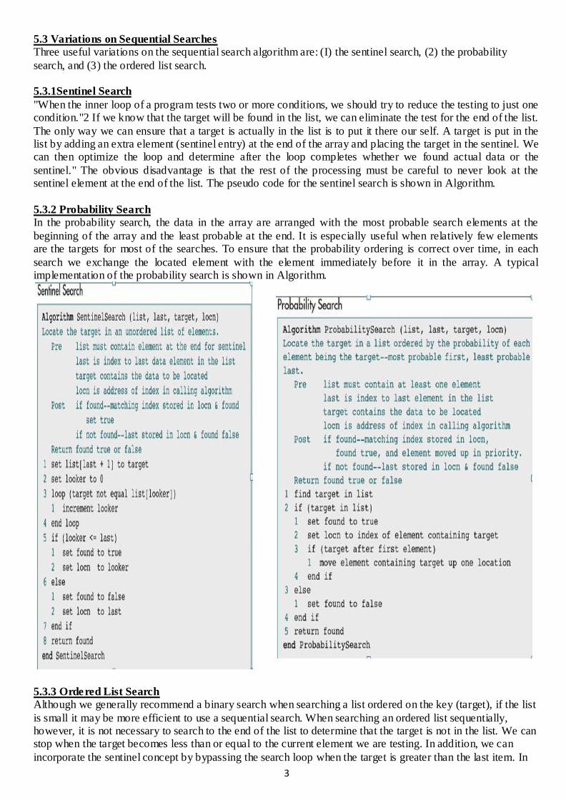
5.3.1Sentinel Search

"When the inner loop of a program tests two or more conditions, we should try to reduce the testing to just one condition."2 If we know that the target will be found in the list, we can eliminate the test for the end of the list.

The only way we can ensure that a target is actually in the list is to put it there our self. A target is put in the list by adding an extra element (sentinel entry) at the end of the array and placing the target in the sentinel. We can then optimize the loop and determine after the loop completes whether we found actual data or the

sentinel." The obvious disadvantage is that the rest of the processing must be careful to never look at the sentinel element at the end of the list. The pseudo code for the sentinel search is shown in Algorithm.

5.3.2 Probability Search

In the probability search, the data in the array are arranged with the most probable search elements at the

beginning of the array and the least probable at the end. It is especially useful when relatively few elements are the targets for most of the searches. To ensure that the probability ordering is correct over time, in each

search we exchange the located element with the element immediately before it in the array. A typical implementation of the probability search is shown in Algorithm.

5.3.3 Ordered List Search

Although we generally recommend a binary search when searching a list ordered on the key (target), if the list

is small it may be more efficient to use a sequential search. When searching an ordered list sequentially, however, it is not necessary to search to the end of the list to determine that the target is not in the list. We can stop when the target becomes less than or equal to the current element we are testing. In addition, we can

incorporate the sentinel concept by bypassing the search loop when the target is greater than the last item. In

4

other words, when the target is less than or equal to the last element, the last element becomes a sentinel,

allowing us to eliminate the test for the end of the list. Although it can be used with array implementations, the ordered list search is more commonly used when

searching linked list implementations. The pseudo code for searching an ordered array is found in Algorithm.

5.4 Binary Search

The sequential search algorithm is very slow. If we have an array of 1000 elements, we must make 1000

comparisons in the worst case. The· binary search starts by testing the data in the element at the middle of the array to determine if the target is in the first or the second half of the list.

mid = (begin + end) / 2 If it is in the first half, we do not need to check the second half. If it is in the second half, we do not need to

test the first half. In other words, we eliminate half the list from further consideration with just one comparison. We repeat this process, eliminating half of the remaining list with each test, until we find the target or determine that it is not

in the list. To find the middle of the list, we need three variables: one to identify the beginning of the list, one to identify

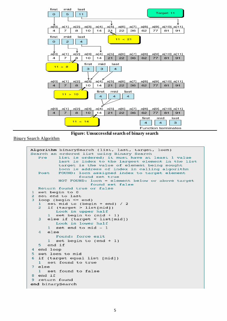
the middle of the list, and one to identify the end of the list. We analyze two cases here: the target is in the list and the target is not in the list.

Figure: Successful search of binary search

5

Figure: Unsuccessful search of binary search

Binary Search Algorithm

6

5.5 Analyzing Search Algorithms

a) For Sequential Search The basic loop for the sequential search is shown below.

The efficiency of the sequential search is O(n).

The search efficiency for the sentinel search is basically the same as for the sequential search. Although the

sentinel search saves a few instructions in the loop, its design is identical. Therefore, it is also an O(n). b) The binary search locates an item by repeatedly dividing the list in half. Its loop is:

This loop obviously divides, and it is therefore a logarithmic loop.

The efficiency is the binary search is O(log n).

The comparison of sequential search & binary search is as follows:

5.6 Hashed List Searches

5.6.1 Basic concept:

In a hashed search, the key, through an algorithmic function, determines the location of the data. We use a hashing algorithm to transform the key into the index that contains the data we need to locate. Another way to describe hashing is as a key-to-address transformation in which the keys map to addresses in a

list. Hashing is a key-to address mapping process.

7

The memory that contains all of the home addresses is .known as the prime area.

The address produced by the hashing algorithm is known as the home address.

A collision occurs when a hashing algorithm produces an address for an insertion key and that address is already occupied.

5.7 Hashing Methods

5.7.1 Direct Method

In direct hashing the key is the address without any algorithmic manipulation. The data structure must

therefore contain an element for every possible key. The situations in which you can use direct hashing are limited.

5.7.2 Subtraction Method

Sometimes keys are consecutive but do not start from 1. For example, a company may have only 100 employees, but the employee numbers start from 1001 and go to 1100. In this case we use subtraction

hashing, a very simple hashing function that subtracts 1000 from the key to determine the address. The direct and subtraction hash functions both guarantee a search effort of one with no collisions.

They are 'one-to-one hashing methods: only one key hashes to each address.

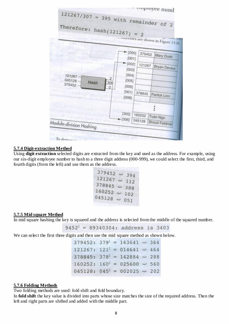
5.7.3 Modulo-division Method

Also known as division remainder, the modulo-division method divides the key by the array size and uses the remainder for the address. This method gives us the simple hashing algorithm shown below in which listSize

is the number of elements in the array:

8

5.7.4 Digit-extraction Method

Using digit extraction selected digits are extracted from the key and used as the address. For example, using

our six-digit employee number to hash to a three digit address (000-999), we could select the first, third, and fourth digits (from the left) and use them as the address.

5.7.5 Mid square Method

In mid square hashing the key is squared and the address is selected from the middle of the squared number.

We can select the first three digits and then use the mid square method as shown below.

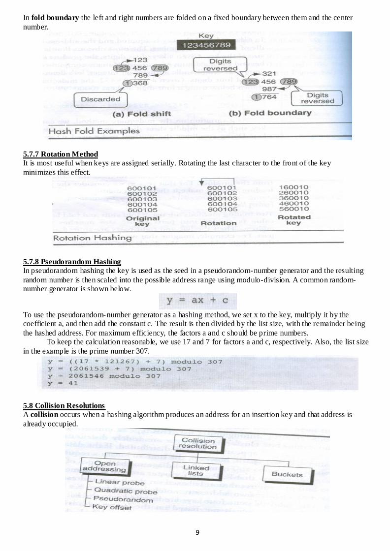
5.7.6 Folding Methods

Two folding methods are used: fold shift and fold boundary.

In fold shift the key value is divided into parts whose size matches the size of the required address. Then the left and right parts are shifted and added with the middle part.

9

In fold boundary the left and right numbers are folded on a fixed boundary between them and the center

number.

5.7.7 Rotation Method

It is most useful when keys are assigned serially. Rotating the last character to the front of the key

minimizes this effect.

5.7.8 Pseudorandom Hashing

In pseudorandom hashing the key is used as the seed in a pseudorandom-number generator and the resulting

random number is then scaled into the possible address range using modulo-division. A common random-number generator is shown below.

To use the pseudorandom-number generator as a hashing method, we set x to the key, multiply it by the coefficient a, and then add the constant c. The result is then divided by the list size, with the remainder being

the hashed address. For maximum efficiency, the factors a and c should be prime numbers. To keep the calculation reasonable, we use 17 and 7 for factors a and c, respectively. Also, the list size

in the example is the prime number 307.

5.8 Collision Resolutions

A collision occurs when a hashing algorithm produces an address for an insertion key and that address is

already occupied.

10

Concepts

a) The load factor of a hashed list is· the number of elements in the list divided by the number of physical elements allocated for the list, expressed as a percentage. Traditionally, load factor is assigned the symbol

alpha (α). The formula in which k repesents the number of filled elements in the list and n represents the total number of elements allocated to the list is

b) Computer scientists have identified two distinct types of clusters. (i) Primary clustering occurs when data cluster around a home address. Primary clustering is easy to

identify. (ii) Secondary clustering occurs when data become grouped along a collision throughout a list. This type of

clustering is not easy to identify.

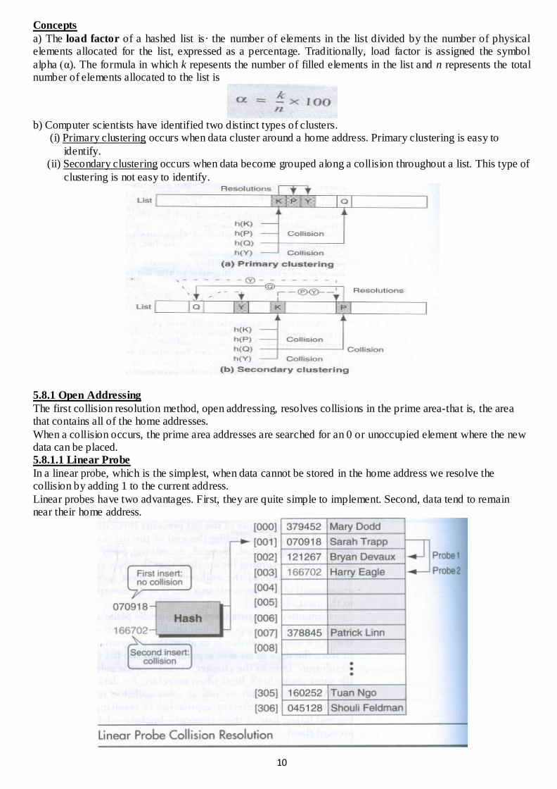
5.8.1 Open Addressing

The first collision resolution method, open addressing, resolves collisions in the prime area-that is, the area that contains all of the home addresses.

When a collision occurs, the prime area addresses are searched for an 0 or unoccupied element where the new data can be placed. 5.8.1.1 Linear Probe

In a linear probe, which is the simplest, when data cannot be stored in the home address we resolve the collision by adding 1 to the current address.

Linear probes have two advantages. First, they are quite simple to implement. Second, data tend to remain near their home address.

11

5.8.1.2 Quadratic Probe

In the quadratic probe, the increment is the collision probe number squared. Thus for the first probe we add 12, for the second collision probe we add 22, for the third collision probe we

add 32, and so forth until we either find an empty element or we exhaust the possible elements.

5.8.1.3 Pseudorandom Collision Resolution

Pseudorandom collision resolution uses a pseudorandom number to resolve the collision. We now use it a collision resolution method. In this case, rather than use the key as a fac tor in the random-number calculation, we use the collision address.

We now resolve the collision using the following pseudorandom-number generator, where a is 3 and c is 5:

5.8.1.4 Key Offset

Key offset is a double hashing method that produces different collision paths for different keys. Whereas the

pseudorandom-number generator produces a new address as a function of the previous address, key offset calculates the new address as a function of the old address and the key. One of the simplest versions simply adds the quotient of the key divided by the list size to the address to

determine the next collision resolution address, as shown in the formula below.

12

Example:

5.8.2 Linked list Collision Resolution

A linked list is ordered collection of data in which each element contains the location of next element. It uses two storage areas: the prime area and the overflow area.

Each element in the prime area contains an addtional field-a link head pointer to a linked list of overflow data in the overflow area. When a collision occurs, one element is stored in the prime area and chained to its corresponding linked list in the overflow area.

Although the overflow area can be any data structure, it is typically implemented as a linked list in dynamic memory.

The linked list data can be stored in any order, but a last in- first out (LIFO) sequence-or a key sequence is the most common.

5.8.3 Bucket Hashing

Another approach to handling the collision problems is bucket hashing, in which keys are hashed to buckets,

nodes that accommodate multiple data occurrences. Because a bucket can hold multiple data, collisions are postponed until the bucket is full.