A Height–Diameter Curve for Longleaf PinePlantations in the Gulf Coastal Plain

Daniel Leduc and Jeffery Goelz

Tree height is a critical component of a complete growth-and-yield model because it is one of the primary components used in volume calculation. To developan equation to predict total height from dbh for longleaf pine (Pinus palustris Mill.) plantations in the West Gulf region, many different sigmoidal curve forms,weighting functions, and ways of expressing height and diameter were explored. Most of the functional forms tried produced very similar results, but ultimatelythe form developed by Levakovic was chosen as best. Another useful result was that scaling diameters by the quadratic mean diameter on a plot and heightby the average height of dominant and codominant trees in the target stand resulted in dramatically better fits than using these variables in their raw forms.

Keywords: Pinus palustris, nonlinear models, model evaluation

An important component of a growth-and-yield model is therelationship between dbh (4.5 ft above ground) and thetotal height of individual trees. The US Forest Service lab-

oratory at Pineville, Louisiana, has collected over 65 years of longleafpine plantation growth information from seven studies within theGulf Coastal plain. The primary purpose of this collection is todevelop a regional growth-and-yield model for thinned and un-thinned plantations of longleaf pine (Pinus palustris Mill.). An im-portant component of a regional growth-and-yield model is theability to supply heights for trees where only diameter is known.Total height is both an important descriptive individual tree variableand also is necessary to calculate tree volume or other product yields.Height predictions can be used both in this regional model and inother situations where only diameters were measured.

Model development is frequently not as orderly as one would likebecause the true mathematical relationship is seldom known, andthere are infinite possible approximations for the true model. Curtis(1967) examined many forms of height–diameter equations andultimately suggested that “any reasonable and moderately flexiblecurve” will give similar results. Complex mathematical functions aremuch easier to fit now than in 1967, so a current evaluation of manymodel forms that were formerly used by other researchers was con-ducted. The necessary assumptions for valid regression models andthe possible scaling of key variables were also evaluated.

Recently, several researchers, including Sharma and Parton(2007), Calama and Montero (2004), Trincado et al. (2007), andJayaraman and Zakrzewski (2001), have begun to use mixed-effectsmodels for height–diameter relationships. In particular, Calamaand Montero (2004) mention that this is just one of several methodsto capture the variability in different stands and the same stand overtime. Mixed-effects models estimate fixed parameters for the generalmodel and then use calibration data such as a few measured treeheights to achieve specificity for a given stand. This is a reasonableapproach, but the main purpose of the model presented here is for

height estimation in a comprehensive growth-and-yield modelwhere there are no measured heights available. For this reason, themodel fitted here relies on quadratic mean diameter and the heightof dominant and codominant trees to achieve the required specific-ity.

MethodsData

Two hundred sixty-seven sample plots of various sizes were dis-tributed in southern Alabama, Mississippi, Louisiana and easternTexas and repeatedly measured, resulting in 2,005 plot-age combi-nations, or 26,490 useable measured tree observations. The studiescombined to create this data set are described in Table 1, and themeans and ranges of important variables are shown in Table 2. Thestudies are further described in Goelz and Leduc (2001) and Goelzet al. (2004).

Model DevelopmentTo select the best model form, the literature was searched for

sigmoidal and other curves that have been previously used to predictheight from diameter. Table 3 shows the 41 curve forms found fortesting and comparison, along with their sources. Regardless of anyeffect on goodness of fit, some modifications were made to make allof the equations more closely match the reality of height versus dbhmodels. The first modification was suggested by Meyer (1940), andit is setting the minimum height to be 4.5 ft. Furthermore, becauseany tree having a measurable dbh cannot have zero diameter at thispoint, in all models the diameter at 4.5 ft was set to 0.5 inches. Thisis a reasonable approximation for longleaf pine, which has a thickterminal bud.

All of the test equations were fit to diameter and height in theiroriginal units, but it was soon discovered that a dramatically im-proved fit could be obtained by using relative diameter and relativeheight. The relative dbh used was obtained by subtracting 0.5 from

Manuscript received April 24, 2007; accepted March 30, 2009.

Daniel Leduc (dleduc@fs.fed.us) and Jeffery Goelz, Alexandria Forestry Center, US Forest Service, 2500 Shreveport Hwy., Pineville, LA 71360. We acknowledge the many technicianswho helped to collect the 65 years’ worth of data used in this model. Valuable comments on the manuscript were provided by Boris Zeide, James D. Haywood, and Bernard Parresol,as well as the anonymous reviewers provided by the journal.

Copyright © 2009 by the Society of American Foresters.

164 SOUTH. J. APPL. FOR. 33(4) 2009

AB

ST

RA

CT

dbh and then dividing the result by the quadratic mean dbh of thatplot. Similarly, 4.5 was subtracted from tree height and the resultwas divided by the average height of dominant and codominanttrees on the plot. Thus, the height prediction equation is specified as

h � 4.5 � �Hd � 4.5� � f ��d � 0.5�/Dq], (42)

where h is total tree height, d is dbh in inches, Hd is average height ofdominant and codominant trees in feet, Dq is the quadratic meandbh in inches for a plot, and f(x) is the equation form being tested.

The standard regression assumptions of independence, normal-ity, and homogeneous variance were examined. It is expected thatthe data used will be autocorrelated since they include many treesfrom the same plots and the same trees measured over time. Viola-tion of this assumption will not affect the parameter estimates, butcalculated variances are most likely underestimated (West 1995). Alldata were used in fitting, since it was felt that the benefits of usingthe available large and diverse data set outweighed the deficiencies,especially given that all equations were fit with the same data. How-ever, results were confirmed with independent observations in sub-sets of the larger data set created by selecting only one tree at onetime from each plot. The assumptions of normality and homogene-ity could also not be shown statistically in the full data set, but theywere shown to be true in most (all homogeneous and 7 of 10 nor-mal) of the independent subsets.

Not all of the equations selected for evaluation are simple func-tions of x and y. Some include other stand variables and someinclude parameters that could be taken as population or stand vari-ables such as the maximum and/or minimum value of dbh or height.These equations were tested with individual plot values and fixedpopulation values. To maximize goodness of fit, the final versions ofEquation 26 uses plot-specific values for xmin and xmax, and Equa-tion 41 uses fixed population values for xmin, xmax, and ymin

(Table 3).After each equation was fit, the parameters were examined to

see whether they were significantly different from 0 in all param-eters and 1 or �1 in those parameters that are multipliers, non-significant parameters at the � � 0.05 level were dropped, andthe equations were refitted. If more than one parameter was

dropped, previously dropped parameters were checked again forinclusion.

In addition to removing nonsignificant parameters, additions ofstand and tree descriptor variables were tried on the published formof the best equation to see whether it could be made better. Thevariables thinning (yes or no), stand density index, trees per acre,basal area, age, and crown class were tested by using simple additivemodifications to the base models.

Most equations were fit using nonlinear regression in PROCNLIN from the SAS Institute (1994). Usually Newton’s methodwas used to find parameters, but when difficult fits were encoun-tered other techniques were used as needed. There was actuallyone equation that always failed to converge in SAS and could befit only using the simplex method as coded in NONLIN (Leduc1986).

Model EvaluationThe primary factor used to evaluate this set of equations was root

mean squared error (RMSE). Fit index, a number comparable to r2

in linear regression (Schlaegel 1981) is also presented, since it iseasier to interpret. However, it will be shown that there is littledifference between equations using just these criteria, so the five bestequations were also checked for bias, mean squared error and abso-lute median difference with cross-validation, and mean squared er-ror on repeated independent sets of data, as explained below. Eventhough relative values were used in fitting many of these equations,the results were always converted back to actual tree heights beforedeviations were calculated.

Because “splitting a sample into two pieces cannot substitute fortrue attempts at replication” (Hursch 1991), the data were not splitinto a set for fitting and a set for testing. All of the data were used forfitting the models. Although it is not a substitute for true replication,model stability was tested for the five best models by cross-validatingbased on study. This extra level of testing was done on only the bestmodels since the purpose of this test was to determine whether anyof these models is less stable than the others that are closely matched.In this test, each study was excluded from the fitting dataset and themodels were fit with this reduced data. Deviations (predicted minusactual) of the excluded study data were recorded, and this processwas repeated, excluding each study in turn. The RMSE, mean bias,and median absolute deviation were calculated for all testedobservations.

Although the complete data set was used in all of the initial fitsand for the final results, because it is known that our data are corre-lated within plots and across years, the best five equations were alsofitted to a subset of data with only one tree from each plot. This fitwas repeated 10 times for each equation, and the resulting meansquared errors were compared for each repetition.

Table 1. Description of West Gulf planted longleaf studies used in this report. Observations are the number of data points obtained fromthe combination of all available trees on all plots for all of the times that a tree was measured.

Title Citation States Observations

Burning, pruning, and thinning in a longleaf spacing plantation (unburned portion) Enghardt (1966) LA 3,634Growth and yield of planted longleaf pine at Sunset Tower Lohrey et al. (1987) LA 1,124Burning, pruning, and thinning in a longleaf spacing plantation (burned portion) Enghardt (1966) LA 6,489Effect of age and residual basal area on growth and yield of planted longleaf pine on

a good siteLohrey (1971) MS 1,938

Growth and yield of planted longleaf pine on medium and poor sites Lohrey (1972) TX 5,521Yields of unthinned longleaf pine plantation on cutover sites in the west gulf region Lohrey (1975) TX, LA 5,311Early longleaf plantation growth on machine-planted prepared sites Boyer and Kush (2004) AL, FL 2,473

Table 2. Descriptive statistics for the data used in model fitting.Stand density index is based upon an exponent of 1.605.

Variable Mean Range

Dbh (in.) 9.4 0.6–23.7Total height (ft) 62.5 5.0–107.5Age (years) 36.5 5–65Basal area per acre (ft2) 109.7 1.8–2566Trees per acre 312.6 20–1550Base age 50 site index (ft) 82.4 62.6–100.8Stand density index 210.0 9.0–497.2

SOUTH. J. APPL. FOR. 33(4) 2009 165

ResultsAs mentioned in the section on model development, all of the

equations were fitted in actual and relative units. Because the use ofrelative units produced such overwhelmingly superior results, final

comparisons were made only in terms of the equations fit withrelative units. In fact, the best equation using actual units, Equation26, was slightly worse than the 28th best equation using relativeunits. When Equation 26 was excluded from the comparison, all

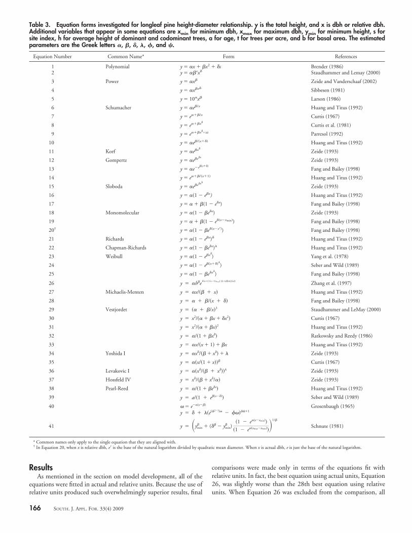
Table 3. Equation forms investigated for longleaf pine height-diameter relationship. y is the total height, and x is dbh or relative dbh.Additional variables that appear in some equations are xmin for minimum dbh, xmax for maximum dbh, ymin for minimum height, s forsite index, h for average height of dominant and codominant trees, a for age, t for trees per acre, and b for basal area. The estimatedparameters are the Greek letters �, �, �, �, �, and �.

Equation Number Common Name* Form References

1 Polynomial y � �x � �x2 � �s Brender (1986)2 y � ��xx� Staudhammer and Lemay (2000)

3 Power y � �x� Zeide and Vanderschaaf (2002)

4 y � �x�x� Sibbesen (1981)

5 y � 10�x� Larson (1986)

6 Schumacher y � �e�/x Huang and Titus (1992)

7 y � e���/x Curtis (1967)

8 y � e���x�Curtis et al. (1981)

9 y � e���x���b Parresol (1992)

10 y � �e�/(x��) Huang and Titus (1992)

11 Korf y � �e�x�Zeide (1993)

12 Gompertz y � �e�e�xZeide (1993)

13 y � �e�e�(x��)Fang and Bailey (1998)

14 y � e���/(x�1) Huang and Titus (1992)

15 Sloboda y � �e�e�x�

Zeide (1993)

16 y � �(1 � e�x) Huang and Titus (1992)

17 y � � � �(1 � e�x) Fang and Bailey (1998)

18 Monomolecular y � �(1 � �e�x) Zeide (1993)

19 y � � � �(1 � e�(x�xmin)) Fang and Bailey (1998)

20† y � �(1 � �e�(x�e�)) Fang and Bailey (1998)

21 Richards y � �(1 � e�x)� Huang and Titus (1992)

22 Chapman-Richards y � �(1 � �e�x)� Huang and Titus (1992)

23 Weibull y � �(1 � e�x�) Yang et al. (1978)

24 y � �(1 � e�(x��)�) Seber and Wild (1989)

25 y � �(1 � �e�x�) Fang and Bailey (1998)

26 y � �h�e �/a��1/x�1/xmax) (��(ln(t)/a)) Zhang et al. (1997)

27 Michaelis-Menten y � �x/�� � x� Huang and Titus (1992)

28 y � � � �/�x � �� Fang and Bailey (1998)

29 Vestjordet y � �� � �/x�3 Staudhammer and LeMay (2000)

30 y � x2/�� � �x � �x2� Curtis (1967)

31 y � x2/�� � �x�2 Huang and Titus (1992)

32 y � �/�1 � �x�� Ratkowsky and Reedy (1986)

33 y � �x/�x � 1� � �x Huang and Titus (1992)

34 Yoshida I y � �x�/�� � x�� � � Zeide (1993)

35 y � ��x/�1 � x��� Curtis (1967)

36 Levakovic I y � ��x�/�� � x���� Zeide (1993)

37 Hossfeld IV y � x�/�� � x�/�� Zeide (1993)

38 Pearl-Reed y � �/�1 � �e�x� Huang and Titus (1992)

39 y � a/�1 � e��x���� Seber and Wild (1989)

40 � e��(x��)

y � � � ��e�2�1� � ���1Grosenbaugh (1965)

41 y � �ymin� � (�� � ymin

� )�1 � e��x�xmin��

�1 � e��xmax�xmin���1/�

Schnute (1981)

* Common names only apply to the single equation that they are aligned with.† In Equation 20, when x is relative dbh, e� is the base of the natural logarithm divided by quadratic mean diameter. When x is actual dbh, e is just the base of the natural logarithm.

166 SOUTH. J. APPL. FOR. 33(4) 2009

relative-unit equations were better than all of the actual-unit equa-tions. Equation 26 (in Table 3) is unique in that it includes Hd as amultiplier, making it somewhat similar to the relative-unit equa-tions. RMSE and fit index of the tested models are shown in Table4. There is very little difference in the goodness of fit of the equa-tions using relative units, and all of these equations tested had fitindices that differed by less than 0.05. Nonetheless it is desirable topick a single best equation, so ease of fit, stability, performance onindependent data, and the use of auxiliary variables were used toconclude that model form 36, attributed to Levakovik by Zeide(1993), was best. With the modifications suggested earlier, the finalmodel based on Equation 36 is as follows:

h � 4.5 � �Hd � 4.5�

� �� ��d � 0.5�/Dq��

� � ��d � 0.5�/Dq��� �

� �, (43)

where �, �, �, and � are the estimated parameters equal to 1.0491,0.2172, 0.2541, and 4.0543, respectively, and � is a random error,�N(0, 2).

Statistics resulting from the fit of the parameters are shown inTable 5, and Figure 1 is a graph of some of the height-dbh relation-ships possible with this model.

A numerical example will illustrate the ease of applying this equa-tion. This example will assume that we have a stand with a quadraticmean diameter of 11.6 inches, an average height of dominant andcodominant trees of 90.3 ft, and a tree with a dbh of 11 inches.Although the equation appears complex, solving this equation issimply a matter of plugging in the estimated parameters and desiredvalues, which results in the following equation:

h � 4.5 � �90.3 � 4.5�

� 1.0491� ��11.0 � 0.5�/11.6�0.2541

0.2172 � ��11.0 � 0.5�/11.6�0.2541� 4.0543

.

(44a)

dbh (inches)

PredictedHeight(feet)

Figure 1. Example curves produced from the final four-parameterequation. Six curves are shown with different base age 50 siteindices (SI) in feet, ages in years, and quadratic mean diameters(QMD) in inches.

Table 4. Statistics measuring the goodness of fit for equationsusing relative height and relative dbh. The results are ranked byroot mean squared error (RMSE).

ModelTerms in

model RMSE Fit index

36 4 4.14889 0.956140 reduced 3 4.15479 0.956022 reduced 4 4.15509 0.956015 4 4.15601 0.955912 3 4.15762 0.955913 3 4.15762 0.955925 4 4.16011 0.955934 4 4.16163 0.955838 3 4.16310 0.955839 3 4.16310 0.955824 reduced 3 4.16389 0.955823 3 4.16389 0.955841 3 4.17067 0.955621 3 4.17578 0.955526 5 4.19600 0.955130 3 4.20049 0.95508 3 4.20749 0.9548

32 3 4.20837 0.954837 3 4.20837 0.954819 3 4.23223 0.954317 3 4.23223 0.954318 3 4.23223 0.954320 3 4.23223 0.95434 3 4.25580 0.95389 4 4.26700 0.95362 3 4.28252 0.9532

11 3 4.29043 0.953010 3 4.34428 0.95196 2 4.37089 0.95137 2 4.37089 0.9513

28 3 4.41979 0.950216 2 4.43718 0.949831 2 4.50779 0.94821 3 4.66842 0.9444

27 2 4.69898 0.943729 2 4.80634 0.941135 2 4.86111 0.939733 2 5.19380 0.93123 2 5.37488 0.92635 2 5.37488 0.9263

14 2 5.64446 0.9187

Table 5. Statistics that describe the estimated parameters forEquation 43.

Parameter EstimateApproximatestandard error

� 1.0491 0.00184� 0.2172 0.00472� 0.2541 0.00935� 4.0543 0.09710

SOUTH. J. APPL. FOR. 33(4) 2009 167

This simplifies to

h � 4.5 � 85.8

� 1.0491� �0.9052�0.2541

0.2172 � �0.9052�0.2541� 4.0543

(44b)

and further to

h � 4.5 � 85.8 � 1.0491� 0.6677

0.2172 � 0.6677�4.0543

(44c)

then

h � 4.5 � 85.8 � 1.0491 � 0.9309, (44d)

with the final result being 88.3 ft. The actual tree from which thesestarting parameters came has a total height of 89 ft. Of course, onewould not normally do this calculation by hand, but rather put theformula into a computer program for instant calculation.

The top five equations were cross-validated by leaving out onestudy at a time and then applying the equation to the left-out study,and the results are presented in Table 6. Equation 36 remained thebest model by a very small margin in root mean square error andmedian absolute difference, but it had a slightly higher bias thanmodel forms 12 and 22.

As mentioned above, the full set of data very likely has manycorrelated observations. Using only a single observation from eachplot and repeating this exercise 10 times, the top five equations wererefit, resulting in model form 36 having the lowest RMSE in 5 of the10 fits. Although model form 36 was not always best, it is, onaverage, slightly better than the other forms. This in shown in Table7, where all of the RMSE values calculated are standardized bydividing by the RMSE of model form 36. Values above 1.0 are lesserfits, and values below 1.0 are better. Whereas other forms are some-times better for a given sample, on average, form 36 is best. How-ever, the difference is very slight, as shown by the nearness of allvalues to 1.0. Since the variance of the estimate made with the fulldata set is potentially too low, it is useful to note that the highestestimate of RMSE for model form 36 using these independent datasets is 4.66 and the corresponding fit index is 0.943, still a high-quality fit.

As mentioned above, thinning, stand density index, trees peracre, basal area, age, and crown class were tested to see whether theiraddition improved the base model. In all cases, there was a signifi-cant improvement (� � 0.05) in fit. However, when the extendedequations were compared with the base equations, there was littlepractical improvement. The largest total height difference observedwith the addition of thinning, stand density index, trees per acre,

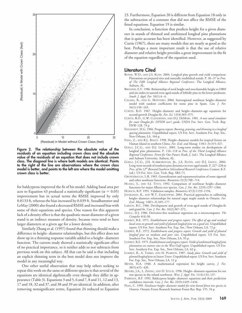
basal area, or age is 2.2 ft, but the average is only 0.09 ft. Crown classproduced some differences as large as 9.4 ft, with an average differ-ence of 0.02 ft, but results were about equally likely to be better orworse (Figure 2). In the interest of parsimony, it was decided toavoid these model extensions.

Discussion and ConclusionsEquation 43 is the best equation that we could find for predicting

the total height of longleaf pine trees from their dbh. However, thereis very little difference between any of the equations evaluated thatused relative diameter and height.

The equations were all fit with and without weighting. Initialwork appeared to indicate that weighting would be required to get acorrect fit for these equations, but further evaluation revealed thatthis was not necessary. A review of the literature that mentionsheteroscedasticity in height–diameter equations revealed onlyHuang and Titus (1992) using a weight of 1/dbh, whereas manyothers, including Parresol (1992), Peng (1999), Zhang et al. (1997),Fang and Bailey (1998), Moore et al. (1996), and Staudhammer andLeMay (2000), found no need for weighting in height–diameterrelationships.

This model was developed to answer the need for height esti-mates in a growth-and-yield projection system that is being devel-oped for thinned and unthinned longleaf pine. The work was notbased on any new theories or methods, but it did reveal severalinteresting observations.

The most obvious of these is that scaling dbh by the quadraticmean dbh in the stand and total height by the average height ofdominant and codominant trees brought about dramatic improve-ments in model fit. Staudhammer and LeMay (2000) discovered asimilar result, but they scaled only the dbh and not the total height,and they used maximum diameter rather than quadratic mean di-ameter. In addition to dividing dbh by the quadratic mean diameteron a plot, maximum diameter was also tried as a divisor, but it wasnot as good with these data. In the best equation, the RMSE usingmaximum diameter was only 4.1972 compared with 4.1489 forquadratic mean diameter.

As mentioned above, adding supplemental variables to the baseequation provided no practical advantage, but previous authors haveemphasized the importance of some supplemental variables. Two ofthem, density and thinning, are worth discussing further.

Zeide and Vanderschaaf (2002) stressed the importance of in-cluding a density term in a height–diameter model. Parresol (1992)found that adding a basal area term to his height–diameter function

Table 6. Statistics measuring the goodness of fit for some of thebest equations when they were cross-validated by study. They aresorted from best to worst using root mean squared error as theranking criterion. The bias is based on predicted minus actualvalues.

EquationRoot mean

squared error BiasMedian absolute

difference

36 4.17238 0.0816 2.5140 reduced 4.17772 0.0818 2.5115 4.17971 0.0827 2.5212 4.18162 0.0813 2.5122 reduced 4.20107 0.0735 2.53

Table 7. Root mean squared error (RMSE) standardized by divid-ing by the RMSE of equation 36 for the best five models using 10randomly selected independent subsets of data.

Sample

Standardized RMSE by equation form

12 15 22 36 40

1 1.000 1.001 0.999 1.000 0.9992 0.999 1.001 0.999 1.000 0.9993 1.002 1.000 1.000 1.000 0.9994 1.003 1.002 1.006 1.000 1.0085 0.999 1.001 0.999 1.000 0.9996 1.003 1.004 1.003 1.000 1.0027 1.007 1.004 1.010 1.000 1.0138 0.999 1.001 1.000 1.000 0.9999 1.000 1.002 1.000 1.000 1.000

10 1.001 1.001 1.004 1.000 1.005Average 1.001 1.002 1.002 1.000 1.003

168 SOUTH. J. APPL. FOR. 33(4) 2009

for baldcypress improved the fit of his model. Adding basal area peracre to Equation 43 produced a statistically significant (� � 0.05)improvement but in actual terms the RMSE improved by only0.0133 ft, whereas the bias increased by 0.039 ft. Staudhammer andLeMay (2000) also found a decreased RMSE and increased bias withsome of their equations and species. One reason for this apparentlack of a density effect is that the quadratic mean diameter of a givenstand is an indirect measure of density, because trees tend to havelarger diameters at a given age for a lower density.

Similarly Zhang et al. (1997) found that thinning should make adifference in height–diameter relationships, but this effect does notshow up in a thinning response variable added to a height–diameterfunction. The current study showed a statistically significant effectof no practical importance, so it neither adds to nor subtracts fromprevious work on this subject. All that can be said is that includingan explicit thinning term in the best model does not improve themodel in any meaningful way.

One other useful observation that may help others seeking torepeat this work on the same or different species is that several of theequations are identical algebraically even though they differ in ap-pearance (Table 3). Equations 3 and 5, 6 and 7, 8 and 11, 12 and 13,17 and 18, 32 and 37, and 38 and 39 are identical. In addition, afterremoving nonsignificant terms, Equation 24 reduced to Equation

23. Furthermore, Equation 20 is different from Equation 18 only inthe subtraction of a constant that did not affect the RMSE of thefitted equations. Equation 19 is similar.

In conclusion, a function that predicts height for a given diam-eter in stands of thinned and unthinned longleaf pine plantationsthat is quite accurate has been identified. However, as suggested byCurtis (1967), there are many models that are nearly as good as thebest. Perhaps a more important result is that the use of relativediameter and relative height provides a great improvement in the fitof the equation regardless of the equation used.

Literature CitedBOYER, W.D., AND J.S. KUSH. 2004. Longleaf pine growth and yield comparison:

Plantations on prepared sites and naturally established stands. P. 36–37 in Proc.of The Fifth Longleaf Alliance Regional Conference. The Longleaf Alliance,Auburn, AL.

BRENDER, E.V. 1986. Relationship of total height and merchantable height to DBHand site index in natural even-aged stands of loblolly pine in the lower piedmont.South. J. Appl. For. 10(1):4–6.

CALAMA, R., AND G. MONTERO. 2004. Interregional nonlinear height–diametermodel with random coefficients for stone pine in Spain. Can. J. For.34(1):150–163.

CURTIS, R.O. 1967. Height–diameter and height–diameter–age equations forsecond-growth Douglas-fir. For. Sci. 13(4):365–375.

CURTIS, R.O., G.W. CLENDENEN, AND D.J. DEMARS. 1981. A new stand simulatorfor coast Douglas-fir: DFSIM user’s guide. USDA For. Serv. Gen. Tech. Rep.PNW-128. 79 p.

ENGHARDT, H.G. 1966. Progress report: Burning, pruning, and thinning in a longleafspacing plantation. Unpublished report. US For. Serv. Southern For. Exp. Stn.,New Orleans, LA. 164 p.

FANG, Z., AND R.L. BAILEY. 1998. Height–diameter models for tropical forests onHainan Island in southern China. For. Ecol. and Manag. 110(1–3):315–327.

GOELZ, J.C.G., AND D.J. LEDUC. 2001. Long-term studies on development oflongleaf pine plantations. P. 116–118 in Proc. of the Third Longleaf AllianceRegional Conference. Forest for Our Future, Kush, J. (ed.). The Longleaf Allianceand Auburn University, Auburn, AL.

GOELZ, J.C.G., J.H. SCARBOROUGH, JR., J.A. FLOYD, AND D.J. LEDUC. 2004.Long-term records of southern pine dynamics in even-aged stands. P. 227–228 inProc. of the 12th Biennial Southern Silvicultural Research Conference, Connor, K.F.(ed.). US For. Serv. Gen. Tech. Rep. SRS–71.

GROSENBAUGH, L.R. 1965. Generalization and reparameterization of some sigmoidand other nonlinear functions. Biometrics 21(3):708–714.

HUANG, S., AND S.J. TITUS. 1992. Comparison of nonlinear height–diameterfunctions for major Alberta tree species. Can. J. For. Res. 22(9):1297–1304.

HURSCH, R.P. 1991. Validation samples. Biometrics 47(3):1193–1194.JAYARAMAN, K., AND W.T. ZAKRZEWSKI. 2001. Practical approaches to calibrating

height–diameter relationships for natural sugar maple stands in Ontario. For.Ecol. Manag. 148(1–3):169–177.

LARSON, B.C. 1986. Development and growth of even-aged stands of Douglas-firand grand fir. Can. J. For. Res. 16(2):367–372.

LEDUC, D.J. 1986. Derivative-free nonlinear regression on a microcomputer. TheCompiler 4(4):38.

LOHREY, R.E. 1971. Establishment and progress report: The effect of age and residualbasal area on growth and yield of planted longleaf pine on a good site. Unpublishedreport. US For. Serv. Southern For. Exp. Stn., New Orleans, LA. 72 p.

LOHREY, R.E. 1972. Establishment and progress report: Growth and yield of plantedlongleaf pine on medium and poor sites. Unpublished report. US For. Serv.Southern For. Exp. Stn., New Orleans, LA. 93 p.

LOHREY, R.E. 1975. Establishment and progress report: Yields of unthinned longleaf pineplantations on cutover sites in the West Gulf region. Unpublished report. US For.Serv. Southern For. Exp. Stn., New Orleans, LA. 62 p.

LOHREY, R., A. TIARKS, AND H. PEARSON. 1987. Study plan: Growth and yield ofplanted longleaf pine at Sunset Tower. Unpublished report. US For. Serv. SouthernFor. Exp. Stn., New Orleans, LA. 12 p.

MEYER, H.A. 1940. A mathematical expression for height curves. J. For.38(5):415–420.

MOORE, J.A., L. ZHANG, AND D. STUCK. 1996. Height–diameter equations for tentree species in the inland northwest. West. J. Appl. For. 11(4):132–137.

PARRESOL, B.P. 1992. Baldcypress height–diameter equations and their predictionconfidence intervals. Can. J. For. Res. 22(9):1429–1434.

PENG, C. 1999. Nonlinear height–diameter models for nine boreal forest tree species inOntario. Ontario Forest Research Institute Forest Res. Rep. 155. 34 p.

Figure 2. The relationship between the absolute value of theresiduals of an equation including crown class and the absolutevalue of the residuals of an equation that does not include crownclass. The diagonal line is where both models are identical. Pointsto the right of the line are observations where the crown classmodel is better, and points to the left are where the model omittingcrown class is better.

SOUTH. J. APPL. FOR. 33(4) 2009 169

RATKOWSKY, D.A., AND T.J. REEDY. 1986. Choosing near-linear parameters in thefour-parameter logistic model for radioligand and related assays. Biometrics42(3):575–582.

SAS INSTITUTE INC. 2004. SAS OnlineDoc 9.1.3. Cary, NC: SAS Institute Inc.SCHLAEGEL, B.E. 1981. Testing, reporting, and using biomass estimation models. p.

95–112 in. Proc. of the 1981 Southern Forest Biomass Workshop, Gresham, C.A.(ed.). Belle W. Baruch For. Sci. Institute of Clemson University, Clemson, SC.

SCHNUTE, J. 1981. A versatile growth model with statistically stable parameters. Can.J. Fish. Aquat. Sci. 38(9):1128–1140.

SEBER, G.A.F., AND C.J. WILD. 1989. Nonlinear regression. John Wiley and Sons,New York. 768 p.

SHARMA, M., AND J. PARTON. 2007. Height–diameter equations for boreal treespecies in Ontario using a mixed-effects modeling approach. For. Ecol. Manag.249(3):187–198.

SIBBESEN, E. 1981. Some new equations to describe phosphate sorption by soils. J.Soil Sci. 32:67–74.

STAUDHAMMER, C., AND V. LEMAY. 2000. Height prediction equations usingdiameter and stand density measures. For. Chron. 76(2):303–309.

TRINCADO, G., C.L. VANDERSCHAAF, AND H.E. BURKHART. 2007. Regionalmixed-effects height–diameter models for loblolly pine (Pinus taeda L.)plantations. Eur. J. For. Res. 126(2): 253–262.

WEST, P.W. 1995. Application of regression analysis to inventory data withmeasurements on successive occasions. For. Ecol. Manag. 71(3):227–234.

YANG, R.C., A. KOZAK, AND J.H.G. SMITH. 1978. The potential of Weibull-typefunctions as flexible growth curves. Can. J. For. Res. 8(4):424–431.

ZEIDE, B. 1993. Analysis of growth equations. For. Sci. 39(3):594–616.ZEIDE, B., AND C. VANDERSCHAAF. 2002. The effect of density on the

height–diameter relationship. P. 463–466 in Proc. of the eleventh biennialsouthern silvicultural research conference, Outcalt, K.W. (ed.). US For. Serv. Gen.Tech. Rep. SRS-48.

ZHANG, S., H.E. BURKHART, AND R.L. AMATEIS. 1997. The influence of thinning ontree height and diameter relationships in loblolly pine plantations. South. J. Appl.For. 21(4):199–205.

170 SOUTH. J. APPL. FOR. 33(4) 2009

been used. For example, Jordan and Ducey (2007) measured fourcrown radii, the first in the direction away from the plot center andthe remaining three at 90, 180, and 270° clockwise; Francis (1988)measured eight radii on the directions north, northeast, east, south-east, south, southwest, west, and northwest; and for the UrbanForest Effects model, Nowak et al. (2005) specify crown diametermeasurements in two directions, north–south and east–west. Bigingand Wensel (1988) observed that basal areas for eccentric trees basedon a measurement of the longest axis or on an average that includedthe longest axis yielded less accurate estimates of the true basal areathan estimates of the basal areas based on the length of the minor, orshortest, axis of the bole. Thus, to eliminate any potential bias incrown area estimations or other applications using an estimatedcrown width, further investigation should be made into the interac-tion between crown measurement protocols and the method forcomputing average crown width.

Literature CitedALZER, H. 1996. A proof of the arithmetic mean-geometric mean inequality. Am.

Math. Mon. 103(7):585.BECHTOLD, W.A. 2003. Crown-diameter prediction models for 87 species of

stand-grown trees in the Eastern United States. South. J. Appl. For.27(4):269–278.

BIGING, G.S., AND L.C. WENSEL. 1988. The effect of eccentricity on the estimationof basal area and basal area increment of coniferous trees. For. Sci.34(3):621–633.

BIGING, G.S., AND M. DOBBERTIN. 1995. Evaluation of competition indices inindividual tree growth models. For. Sci. 41(2):360–377.

FOOD AND AGRICULTURE ORGANIZATION (FAO). 2006. Global forest resourcesassessment 2005, progress towards sustainable forest management. FAO For. Pap.147, FAO, Rome, Italy. 320 p.

FRANCIS, J.K. 1988. The relationship of bole diameters and crown widths of sevenbottomland hardwood species. US For. Serv. Res. Note SO-328. 3 p.

GILL, S.J., G.S. BIGING., AND E.C. MURPHY. 2000. Modeling conifer tree crownradius and estimating canopy cover. For. Ecol. Manag. 126:405–416.

GROTE, R,, AND I.M. REITER. 2004. Competition-dependent modeling of foliagebiomass in forest stands. Trees 18(5):596–607.

JENNINGS, S.B., N.D. BROWN., AND D. SHEIL. 1999. Assessing forest canopies andunderstorey illumination: canopy closure, canopy cover and other measures.Forestry 72(1):59–73.

JORDAN, G.J., AND M.J. DUCEY. 2007. Predicting crown radius in eastern white pine(Pinus strobus L.) stands in New Hampshire. North. J. Appl. For. 24(1):61–64.

MARSHALL, D.D., G.P. JOHNSON., AND D.W. HANN. 2003. Crown profile equationsfor stand-grown western hemlock trees in northwestern Oregon. Can. J. For. Res.33:2059–2066.

MCPHERSON, E.G., AND R.A. ROWNTREE. 1988. Geometric solids for simulation oftree crowns. Landsc. Urban Plan. 15:79–83.

NOWAK, D.J., D.E. CRANE, J.C. STEVENS, AND R.E. HOEHN. 2005. The Urban ForestEffects (UFORE) model: Field data collection manual, Ver. 1b. US For. Serv.Northeastern Res. Stn., Syracuse, NY. Available online at www.ufore.org/UFORE_manual.doc; last accessed Dec. 12, 2008.

RIITTERS, K., AND B. TKACZ. 2004. The US Forest Health Monitoring Program. P.669–683 in Environmental monitoring, Wiersma, B. (ed.). CRC Press, BocaRaton, FL.

SPRINZ, P.T., AND H.E. BURKHART. 1987. Relationships between tree crown, stem,and stand characteristics in unthinned loblolly pine plantations. Can. J. For. Res.17(6):534–538.

SUMIDA, A., AND A. KOMIYAMA. 1997. Crown spread patterns for five deciduousbroad-leaved woody species: Ecological significance of the retention patterns oflarger branches. Ann. Bot-London 80(6):759–766.

US FOREST SERVICE. 1999. Forest health monitoring 1999 field methods guide. US For.Serv., National Forest Health Monitoring Program, Research Triangle Park,NC.

ZARNOCH, S.J., W.A. BECHTOLD., AND K.W. STOLTE. 2004. Using crown conditionvariables as indicators of forest health. Can. J. For. Res. 34:1057–1070.

CORRECTION

LEDUC, D., AND J. GOELZ. 2009. A Height–Diameter Curve for Longleaf Pine Plantations in theGulf Coastal Plain South. J. Appl. For. 33(4):164–170.

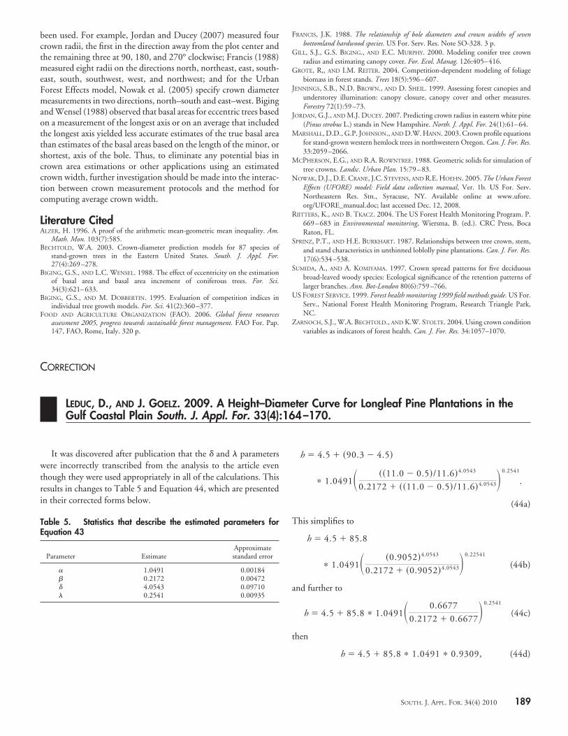
It was discovered after publication that the � and � parameterswere incorrectly transcribed from the analysis to the article eventhough they were used appropriately in all of the calculations. Thisresults in changes to Table 5 and Equation 44, which are presentedin their corrected forms below.

Table 5. Statistics that describe the estimated parameters forEquation 43

Parameter EstimateApproximatestandard error

1.0491 0.00184 0.2172 0.00472� 4.0543 0.09710� 0.2541 0.00935

h � 4.5 � �90.3 � 4.5�

� 1.0491� ��11.0 � 0.5�/11.6�4.0543

0.2172 � ��11.0 � 0.5�/11.6�4.0543� 0.2541

.

(44a)

This simplifies to

h � 4.5 � 85.8

� 1.0491� �0.9052�4.0543

0.2172 � �0.9052�4.0543� 0.22541

(44b)

and further to

h � 4.5 � 85.8 � 1.0491� 0.6677

0.2172 � 0.6677�0.2541

(44c)

then

h � 4.5 � 85.8 � 1.0491 � 0.9309, (44d)

SOUTH. J. APPL. FOR. 34(4) 2010 189