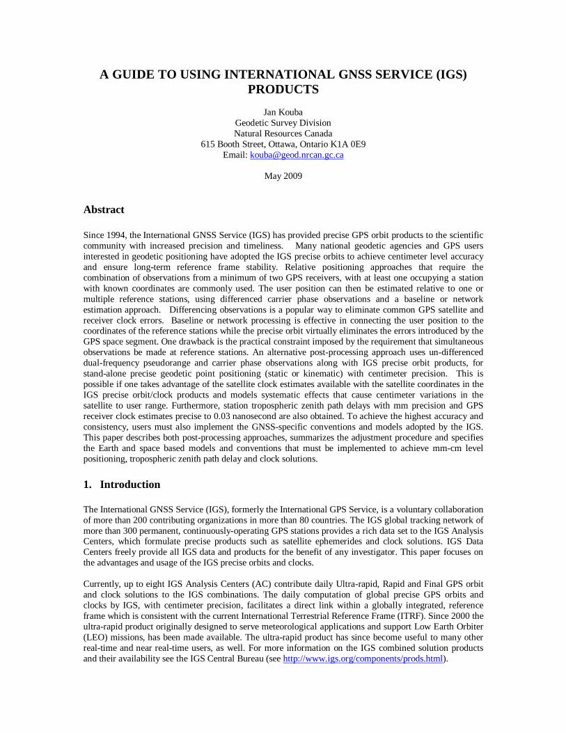
A GUIDE TO USING INTERNATIONAL GNSS SERVICE (IGS)PRODUCTS

Jan KoubaGeodetic Survey DivisionNatural Resources Canada

615 Booth Street, Ottawa, Ontario K1A 0E9Email: kouba@geod.nrcan.gc.ca

May 2009

Abstract

Since 1994, the International GNSS Service (IGS) has provided precise GPS orbit products to the scientificcommunity with increased precision and timeliness. Many national geodetic agencies and GPS usersinterested in geodetic positioning have adopted the IGS precise orbits to achieve centimeter level accuracyand ensure long-term reference frame stability. Relative positioning approaches that require thecombination of observations from a minimum of two GPS receivers, with at least one occupying a stationwith known coordinates are commonly used. The user position can then be estimated relative to one ormultiple reference stations, using differenced carrier phase observations and a baseline or networkestimation approach. Differencing observations is a popular way to eliminate common GPS satellite andreceiver clock errors. Baseline or network processing is effective in connecting the user position to thecoordinates of the reference stations while the precise orbit virtually eliminates the errors introduced by theGPS space segment. One drawback is the practical constraint imposed by the requirement that simultaneousobservations be made at reference stations. An alternative post-processing approach uses un-differenceddual-frequency pseudorange and carrier phase observations along with IGS precise orbit products, forstand-alone precise geodetic point positioning (static or kinematic) with centimeter precision. This ispossible if one takes advantage of the satellite clock estimates available with the satellite coordinates in theIGS precise orbit/clock products and models systematic effects that cause centimeter variations in thesatellite to user range. Furthermore, station tropospheric zenith path delays with mm precision and GPSreceiver clock estimates precise to 0.03 nanosecond are also obtained. To achieve the highest accuracy andconsistency, users must also implement the GNSS-specific conventions and models adopted by the IGS.This paper describes both post-processing approaches, summarizes the adjustment procedure and specifiesthe Earth and space based models and conventions that must be implemented to achieve mm-cm levelpositioning, tropospheric zenith path delay and clock solutions.

1. Introduction

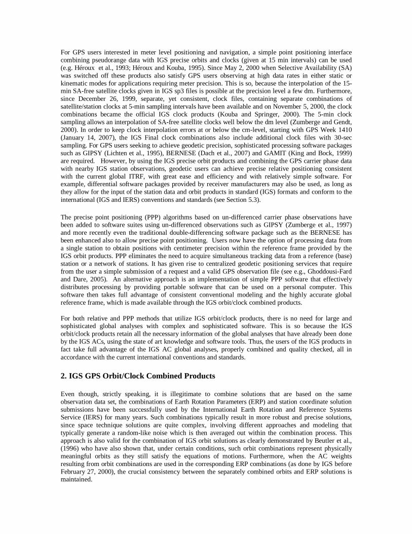
The International GNSS Service (IGS), formerly the International GPS Service, is a voluntary collaborationof more than 200 contributing organizations in more than 80 countries. The IGS global tracking network ofmore than 300 permanent, continuously-operating GPS stations provides a rich data set to the IGS AnalysisCenters, which formulate precise products such as satellite ephemerides and clock solutions. IGS DataCenters freely provide all IGS data and products for the benefit of any investigator. This paper focuses onthe advantages and usage of the IGS precise orbits and clocks.

Currently, up to eight IGS Analysis Centers (AC) contribute daily Ultra-rapid, Rapid and Final GPS orbitand clock solutions to the IGS combinations. The daily computation of global precise GPS orbits andclocks by IGS, with centimeter precision, facilitates a direct link within a globally integrated, referenceframe which is consistent with the current International Terrestrial Reference Frame (ITRF). Since 2000 theultra-rapid product originally designed to serve meteorological applications and support Low Earth Orbiter(LEO) missions, has been made available. The ultra-rapid product has since become useful to many otherreal-time and near real-time users, as well. For more information on the IGS combined solution productsand their availability see the IGS Central Bureau (see http://www.igs.org/components/prods.html).

For GPS users interested in meter level positioning and navigation, a simple point positioning interfacecombining pseudorange data with IGS precise orbits and clocks (given at 15 min intervals) can be used(e.g. Héroux et al., 1993; Héroux and Kouba, 1995). Since May 2, 2000 when Selective Availability (SA)was switched off these products also satisfy GPS users observing at high data rates in either static orkinematic modes for applications requiring meter precision. This is so, because the interpolation of the 15-min SA-free satellite clocks given in IGS sp3 files is possible at the precision level a few dm. Furthermore,since December 26, 1999, separate, yet consistent, clock files, containing separate combinations ofsatellite/station clocks at 5-min sampling intervals have been available and on November 5, 2000, the clockcombinations became the official IGS clock products (Kouba and Springer, 2000). The 5-min clocksampling allows an interpolation of SA-free satellite clocks well below the dm level (Zumberge and Gendt,2000). In order to keep clock interpolation errors at or below the cm-level, starting with GPS Week 1410(January 14, 2007), the IGS Final clock combinations also include additional clock files with 30-secsampling. For GPS users seeking to achieve geodetic precision, sophisticated processing software packagessuch as GIPSY (Lichten et al., 1995), BERNESE (Dach et al., 2007) and GAMIT (King and Bock, 1999)are required. However, by using the IGS precise orbit products and combining the GPS carrier phase datawith nearby IGS station observations, geodetic users can achieve precise relative positioning consistentwith the current global ITRF, with great ease and efficiency and with relatively simple software. Forexample, differential software packages provided by receiver manufacturers may also be used, as long asthey allow for the input of the station data and orbit products in standard (IGS) formats and conform to theinternational (IGS and IERS) conventions and standards (see Section 5.3).

The precise point positioning (PPP) algorithms based on un-differenced carrier phase observations havebeen added to software suites using un-differenced observations such as GIPSY (Zumberge et al., 1997)and more recently even the traditional double-differencing software package such as the BERNESE hasbeen enhanced also to allow precise point positioning. Users now have the option of processing data froma single station to obtain positions with centimeter precision within the reference frame provided by theIGS orbit products. PPP eliminates the need to acquire simultaneous tracking data from a reference (base)station or a network of stations. It has given rise to centralized geodetic positioning services that requirefrom the user a simple submission of a request and a valid GPS observation file (see e.g., Ghoddousi-Fardand Dare, 2005). An alternative approach is an implementation of simple PPP software that effectivelydistributes processing by providing portable software that can be used on a personal computer. Thissoftware then takes full advantage of consistent conventional modeling and the highly accurate globalreference frame, which is made available through the IGS orbit/clock combined products.

For both relative and PPP methods that utilize IGS orbit/clock products, there is no need for large andsophisticated global analyses with complex and sophisticated software. This is so because the IGSorbit/clock products retain all the necessary information of the global analyses that have already been doneby the IGS ACs, using the state of art knowledge and software tools. Thus, the users of the IGS products infact take full advantage of the IGS AC global analyses, properly combined and quality checked, all inaccordance with the current international conventions and standards.

2. IGS GPS Orbit/Clock Combined Products

Even though, strictly speaking, it is illegitimate to combine solutions that are based on the sameobservation data set, the combinations of Earth Rotation Parameters (ERP) and station coordinate solutionsubmissions have been successfully used by the International Earth Rotation and Reference SystemsService (IERS) for many years. Such combinations typically result in more robust and precise solutions,since space technique solutions are quite complex, involving different approaches and modeling thattypically generate a random-like noise which is then averaged out within the combination process. Thisapproach is also valid for the combination of IGS orbit solutions as clearly demonstrated by Beutler et al.,(1996) who have also shown that, under certain conditions, such orbit combinations represent physicallymeaningful orbits as they still satisfy the equations of motions. Furthermore, when the AC weightsresulting from orbit combinations are used in the corresponding ERP combinations (as done by IGS beforeFebruary 27, 2000), the crucial consistency between the separately combined orbits and ERP solutions ismaintained.

The IGS combined orbit/clock products come in various flavors, from the Final, Rapid to the Ultra-Rapid,which became officially available on November 5, 2000 (GPS Week 1087, MJD 5183). The IGS Ultra-Rapid (IGU) products replaced the former IGS predicted (IGP) orbit products (IGS Mail #3229). The IGScombined orbit/clock products differ mainly by their varying latency and the extent of the tracking networkused for their computations. The IGS Final orbits (clocks) are currently combined from up to eight (seven)contributing IGS ACs, using six, largely independent, software packages (i.e. BERNESE, GAMIT, GIPSY,NAPEOS (Dow et al., 1999), EPOS (Gendt et al., 1999) and PAGES (Schenewerk et al., 1999). The IGSFinal orbit/clocks are usually available before the thirteenth day after the last observation. The Rapidorbit/clock product is combined 17 hours after the end of the day of interest. The latency is mainly due tothe varying availability of tracking data from stations of the IGS global tracking network, which use avariety of data acquisition and communication schemes, as well as different levels of quality control. In thepast, the IGS products have been based only on a daily model that required submissions of files containingtracking data for 24-hour periods. In 2000, Data Centers have been asked to forward hourly tracking datato accelerate product delivery. This new submission scheme was required for the creation of an Ultra-Rapid product, with a latency of only a few hours, that should satisfy the more demanding needs of mostreal-time users, including the meteorological community and LEO (Low Earth Orbiter) missions. It isexpected that IGS products will continue to be delivered with increased timeliness in the future (Weber etal., 2002). Development of true real-time products, mostly satellite clock corrections, is underway withinthe IGS Real-Time Pilot Project. For more information on the IGS products and their possible applicationssee e.g. Neilan et al., (1997); Kouba et al., (1998) and Dow et al., (2005).

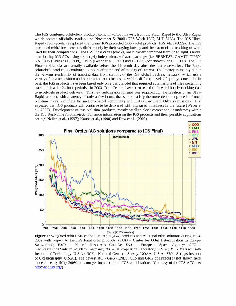
Figure 1: Weighted orbit RMS of the IGS Rapid (IGR) products and AC Final orbit solutions during 1994-2009 with respect to the IGS Final orbit products. (COD – Center for Orbit Determination in Europe,Switzerland; EMR – Natural Resources Canada; ESA - European Space Agency; GFZ –GeoForschungsZentrum Potsdam, Germany; JPL – Jet Propulsion Laboratory, U.S.A.; MIT- MassachusettsInstitute of Technology, U.S.A.; NGS – National Geodetic Survey, NOAA, U.S.A.; SIO - Scripps Instituteof Oceanography, U.S.A.). The newest AC - GRG (CNES, CLS and GRG of France) is not shown here,since currently (May 2009), it is not yet included in the IGS combinations. (Courtesy of the IGS ACC, seehttp://acc.igs.org/)

From Figure 1, one can see that over the past 15 years the precision of the AC Final orbits has improvedfrom about 30 cm to about 1 - 2 cm, with a concomitant improvement in the IGS Final combined orbit. Itis also interesting to note that the IGS Rapid orbit combined product (IGR), with less tracking stations andfaster delivery times, is now more precise than the best AC Final solutions. The precision of thecorresponding AC/IGS ERP solutions has shown similar improvements since 1994. One element that hasreceived less attention is the quality of the GPS satellite clock estimates included in the IGS orbit productssince 1995. Examining the summary plots for IGS Final clock combinations at the IGS AC Coordinator(ACC) web site (http://acc.igs.org/), one can notice that after small biases are removed, the satellite clockestimates produced by different ACs now agree with standard deviations of 0.02 - 0.06 nanosecond (ns) or1 - 2 cm. This is also consistent with the orbit precision. Any biases in the individual IGS satellite clockswill be absorbed into the phase ambiguity parameters that users must adjust. The precise GPS orbits andclocks, weighted according to their corresponding precision (sigmas), are the key prerequisites for PPP,given that the proper measurements are made at the user site and the observation models are implementedcorrectly.

3. Observation equations

The ionospheric-free combinations of dual-frequency GPS pseudorange (P) and carrier-phase observations(Φ) are related to the user position, clock, troposphere and ambiguity parameters according to the followingsimplified observation equations:

ℓ P = ρ + c(dT-dt) + Tr + εP ( 1 )

φℓ = ρ + c(dT-dt) + Tr + N λ + εΦ ( 2 )

Where :ℓ P (P3) is the ionosphere-free combination of P1 and P2 pseudoranges (2.546P1-1.546P2),

ℓ Φ (L3) is the ionosphere-free combination of L1 and L2 carrier-phases (2.546λ1φ1-1.546λ2φ2),dT is the station receiver clock offset from the GPS time,dt is the satellite clock offset from the GPS time,c is the vacuum speed of light,Tr is the signal path delay due to the neutral-atmosphere (primarily the troposphere),N is the non-integer ambiguity of the carrier-phase ionosphere-free combination,λ1, λ2, λ are the of the carrier- phase L1, L2 and L3-combined (10.7cm) wavelengths, respectively,εP, εΦ are the relevant measurement noise components, including multipath.

Symbol ρ is the geometrical range computed by iteration from the satellite position (Xs, Ys, Zs) at thetransmission epoch t and the station position (x, y, z) at the reception epoch T = t +ρ/c, i.e.

)()()(222

zZsyYsxXs −−− ++=ρ .

Alternatively, for relative positioning between two stations (i, j) the satellite clock errors dt can beeliminated simply by subtracting the corresponding observation Eqs. (1) and (2) made from the two stations(i, j ) to the same satellite (k), i.e.:

ℓ Pijk = ∆ρ ij

k+ c∆dTij + ∆Trijk + ∆εPij

k , (3)

ℓ Φijk = ∆ρ ij

k+ c∆dTij + ∆Trijk + ∆Nij

k λ + ∆εΦijk , (4)

here ∆(.)ijk denotes the single difference. By subtracting the observation Eqs. (3) and (4) pertaining to the

stations (i, j) and the satellite k from the corresponding equations of the stations (i, j) to the satellite l, wecan form so called double differenced observation equations, where the station clock difference errors

∆dTij , which are the same for both single differences, are also eliminated (assuming that all channelswithin the receiver, tracking different satellites, share exactly the same clock offset, which is generally true

for GPS where all the satellites use common carrier frequencies but is not usually true for GLONASSwhere satellites broadcast on different carrier frequencies; if the GLONASS channel biases are rather stablein time, the residual clock offset can be absorbed into the phase ambiguity parameters):

ℓ Pijkl = ∆ρ ij

kl + ∆Trijkl + ∆εPij

kl , (5)

ℓΦijkl = ∆ρ ij

kl+ ∆Trijkl + ∆Nij

kl λ+ ∆εΦijkl, (6)

where ∆(.)ijkl represents the respective double difference for the (i, j) station and (k, l) satellite pairs.

Furthermore, the initial L1 and L2 phase ambiguities that are used to evaluate the ionospheric-freeambiguities ∆Nij

kl become integers. This is so since the fractional phase initializations on L1 & L2 for thestation (i, j) and satellite (k, l) pairs, much like station/satellite clock errors, are also eliminated by theabove double differencing scheme. Consequently, once the L1 and L2 ambiguities are resolved, theionospheric-free ambiguities ∆Nij

kl become known and can thus be removed from the equation (6), whichthen becomes equivalent to the pseudorange equation (5), i.e. double differenced phase observations withfixed ambiguities become precise pseudorange observations that are derived from unambiguous precisephase measurement differences. That is why fixed ambiguity solutions yield relative positioning of thehighest possible precision, typically at or below the mm precision level (e.g. Hoffmann-Wellenhof et al.,1992).

The equations (1), (2) and (5), (6) appear to be quite different, with a different number of unknowns anddifferent magnitudes of the individual terms. For example, the double differenced tropospheric delay ∆Trij

kl

is much smaller than the un-differenced Tr, , the noise ∆ε(.)ijkl is significantly larger than the original, un-

differenced noise ε(.), etc. Nevertheless, both un-differenced and double differenced approaches produceidentical results, provided that the same set of un-differenced observations and proper correlation derivedfrom the differencing, are used. In other words, the double difference position solutions with properlypropagated observation weight matrix (see e.g. Hoffmann-Wellenhof et al., 1992), are completelyequivalent to un-correlated, un-differenced solutions where the (satellite/station) clock unknowns aresolved for each observation epoch.

Since we are using the IGS orbit/clock products, the satellite clocks (dt) in Eqs. (1) and (2) can be fixed(considered known) and thus can be removed. Furthermore, expressing the tropospheric path delay (Tr) as aproduct of the zenith path delay (zpd) and mapping function (M), which relates slant path delay to zpd,gives the point positioning mathematical model functions for pseudorange and phase observations:

fP = ρ + c dT + M zpd + εP - ℓ P = 0, ( 7 )

fΦ = ρ + c dT + M zpd + N λ + εΦ - ℓΦ = 0; ( 8 )

The tropospheric path delay (M zpd ) is separated in a predominant and well-behaved hydrostatic part (Mh

zpdh) and a much smaller and volatile wet part (Mw zpdw). While zpdh can be modeled and consideredknown, zpdw has to be estimated. For most precise solutions, temporarily varying zpdh, Mh and Mw have tobe based either on global seasonal models (Boehm et al., 2006; Boehm et al., 2007), numerical weathermodels (Boehm and Schuh, 2004; Kouba, 2007), or alternatively (and potentially more precisely) zpdh canbe computed from measured station atmospheric pressure (see e.g., Kouba, 2009). For a concise summaryof precise zpd modeling, consult the IERS Conventions updated Chapter 9 at:http://tai.bipm.org/iers/convupdt/convupdt_c9.html.

Unlike the Eqs. (1) - (6) that contain unknowns and/or observation differences involving baselines or thewhole station network, the Eqs. (7) and (8), after fixing known satellite clocks and positions, containobservations and unknowns pertaining to a single station only. Note that satellite clock and orbit weightingdoes not require the satellite clock and position parameterizations, since the satellite clock and positionweighting can be effectively accounted for by satellite specific pseudorange/phase observation weighting.So, unless attempting to fix integer ambiguities (see below), it makes little or no sense to solve Eqs. (7) and(8) in a network solution as it would still result in uncorrelated station solutions that are exactly identical toindependent, single station, point positioning solutions. Conversely, if a network station solution with a full

variance-covariance matrix is required, such as is the case of a Regional Network Associated AnalysisCenter (RNAAC) processing (http://www.igs.org/organization/centers.html#RNAAC), only theobservation Eqs. (1) - (6) are meaningful and should be used. Also note that in single point positioningsolutions it is not possible to fix L1, L2 integer ambiguities, unlike for the network solutions utilizingdouble differenced or even un-differenced observations. For un-differenced network solutions, the resolvedL1, L2 double differenced integer ambiguities are used to derive the ionospheric-free real ambiguities andthen the known double differenced integer ambiguities are introduced as condition equations into thecorresponding matrix of the normal equations. An alternative and more efficient approach is to generateseparate pseudorange and phase clocks for GPS satellites, where the phase clocks are made consistent withthe resolved integer L1, L2 phase ambiguities. Then even a single PPP user can resolve and fix integerphase ambiguities without any need of additional station network data (Collins, 2008). It is worth to notethat PPP (Eqs. (7) and (8)) allows position, tropospheric zenith path delay and receiver clock solutions thatare consistent with the global reference system implied by the fixed IGS orbit/clock products. Thedifferential (Eqs. (5) and (6)), on the other hand, does not allow for any precise clock solutions, and thetropospheric zpdw solutions may be biased by a constant (datum) offset, in particular for regional and localbaselines/networks (< 500 km). Thus, such regional/local zpdw solutions, based on double differencenetwork analyses, require external tropspheric zpdw calibration (at least at one station), e.g. by means ofPPP, or the IGS troposheric combined zpd products (Gendt, 1996, 1998; Byun and Bar-Sever, 2009).

4. Adjustment models

For the sake of simplicity, only the point positioning approach is discussed in this section. However, theadjustments of un-differenced or differenced data in network solutions are quite analogous to this rathersimple, yet still precise point positioning case.

Linearization of the observation Eqs. (7) and (8) around the a-priori parameter values and observations (X0,ℓ ) in the matrix form becomes:

A δ + W – V = 0, (9)

where A is the design matrix, δ is the vector of corrections to the unknown parameters X, W = f(X0, ℓ ) isthe misclosure vector and V is the vector of residuals.

The partial derivatives of the observation equations with respect to X, which in the case of PPP consist offour types of parameters: station position (x, y, z), receiver clock (dT), wet troposphere zenith path delay(zpdw) and (non-integer) carrier-phase ambiguities (N), form the design matrix A:

( , ) ( , ) ( , ) ( , ) ( , ) ( , )

( , )

( , ) ( , ) ( , ) ( , ) ( , ) ( , )

( , )

w

w

f X f X f X f X f X f XP P P P P PX X X X X Xx y z jdT zpd

N j 1 nsat

f X f X f X f X f X f X

X X X X X Xx y z jdT zpdN j 1 nsat

A

∂ ∂ ∂ ∂ ∂ ∂

∂ ∂ ∂ ∂ ∂ ∂=

∂ ∂ ∂ ∂ ∂ ∂Φ Φ Φ Φ Φ Φ∂ ∂ ∂ ∂ ∂ ∂

=

=

ℓ ℓ ℓ ℓ ℓ ℓ

ℓ ℓ ℓ ℓ ℓ ℓ

,,,:ρρρ

Zsz

zX

fYsy

yX

fXsx

xX

fwith

−=

∂

∂−=

∂

∂−=

∂

∂

, ,

( , )

w

w

f f fc M 0 or 1

X X X jdT zpdN j 1 nsat

∂ ∂ ∂= = =

∂ ∂ ∂=

( , )

w

x

y

zX dT

zpd

jN j 1 nsat

=

=

.

The least squares solution with a-priori weighted parameter constraints ( oXP ) is given by:

WPT

A1

)APATP0X

(ℓℓ

−+−=δ , ( 10 )

where ℓP

is the observation weight matrix. For un-differenced observations it is usually a diagonal matrix

with the diagonal terms equal to (σo/σP)2 and (σo/σΦ)2 , where σo is the standard deviation of the unit

weight, σP and σΦ are the standard deviations (sigmas) of pseudorange and phase observations,respectively. Typically, σΦ≅ 10 mm and the ratio of σP/σΦ ≥ 100 are used for ionospheric-free un-differenced phase and pseudorange observations. Then the estimated parameters are

δ+= 0XX

⌢,

with the corresponding weight coefficient matrix ( the a priori variance-covariance matrix when σo=1 )1)T

0(1 −+=−= APA

XP

XP

XC

ℓ⌢⌢ . ( 11 )

The weighted square sum of residuals is obtained from the residuals, evaluated from Eq. (9) and theparameter correction vector (Eq. 10) as follows:

VPVX

PTPVTVℓ

T0 += δδ , (12)

or from an alternative, but numerically exactly equivalent expression:

WPVPVT

Vℓ

T= . (13)

Both expressions can be used to check the numerical stability of the solution (Eq. 10). Finally, the aposteriori variance-covariance matrix of the estimated parameters is

1)T0(

2

0−+

∧=Σ APA

XP

X ℓ⌢ σ

, (14)

where the a posteriori variance factor is estimated from the square sum of residuals and the degrees offreedom df = n-u ; (n , u are the number of observations and the number of effective unknowns,respectively):

)(

T2

0un

VPV

−=

∧σ . (15)

The formal variance-covariance matrices Eq. (14) are usually too optimistic (with too small variances),typically by a factor 5 or more, depending on the data sampling and the complexity of error modeling usedin GPS analyses. The longer the data sampling interval and the more sophisticated error modeling are, thesmaller (and closer to 1) the factor tends to be.

A note on non-integer number of degrees of freedom is due at this point, since, in principle, all or none ofthe parameters X0 can be weighted. Thus the trace (u’) of the a priori parameter weight matrix P x

effectively determines an equivalent of the number of observations, so that the effective number ofunknowns u = ux – u’ (ux is the dimension of the parameter vector X0) can be a real number attainingvalues between 0 and ux.. This can make the number of degrees of freedom df = n - u a non integer number.

4.1 Statistical testing, data editing

The simplest statistical testing/data editing usually involves uni-variate statistical tests of the misclosures Wand residuals V that are based on limits equal to a constant multiple (k) of sigmas, i.e. using the probabilityP at the probability level (1-α) and the phase misclosures:

P{ -k σΦ < wΦj < k σΦ } = (1-α); j=1, n (n- number of observations) (16)

where α is the probability that the variable |wΦj| > k σΦ . For example, for the Normal Distribution (ND)and the 99% probability level k = 2.58. The Chebyshev inequality, which is consistent with a wide range oferror distributions, states that for all general (non Normal) error distributions the probability P that thevariable is within the limits of ± k σΦ is greater or equal to (1-α), provided that k= (α)-1/2 (e.g. Hamilton,1964). When α =0.05 is assumed then k=4.47. That is why the sigma multipliers of 5 and 3 are usuallychosen for the outlier testing of misclosures and residuals, respectively. Note that in the above tests, strictlyspeaking, a posteriori estimates of the observation sigmas should be used, i.e.�����

0

∧=

∧. (17)

When assuming the ND, the square sum of residuals (12), (13) are distributed according to the well knownχ2 variable, thus the square sums can be effectively tested, at the (1-α) probability level, against the

statistical limit of 2

0

∧σ χ2

df,α/2. This test can also be applied to the square sum of weighted parameters (thefirst term on the right hand side of Eq. (12)), or to other subgroups of the weighted parameters and/orresiduals. E.g. the residuals pertaining to a specific satellite and/or station can be tested in this way.Alternatively, the above χ2 test could be applied to a single epoch increment of the square sum of residualsEqs. (12) or (13). The power of this test is increasing with the decreasing group size (i.e. the increment ofthe number of degrees of freedom). For a single residual and/or parameter this χ2 test becomes exactlyequivalent to the well-known Student’s tα test (equivalent to the above ND for large number of degrees offreedom, i.e. when df => �), since χ2

1,α = (tα) 2. For more details and an extended bibliography onstatistical testing in geodetic applications see e.g. Vaníček and Krakiwsky (1986).

Data editing and cycle slip detection for un-differenced, single station observations is, indeed, a majorchallenge, in particular during periods of high ionospheric activities and/or station in the ionosphericallydisturbed polar or equatorial regions. This is so, since the difference between L1 and L2 phase observationsare usually used to check and edit cycle slips and outliers. However, in the extreme cases, this editingapproach would need data sampling higher than 1 Hz in order to safely recognized or edit cycle slips oroutliers and such high data samplings are not usually available. (Note that within a geodetic receiver, atleast in principle, it should be possible to do an efficient and reliable data cleaning/editing based on the (L1-L2) or L1, L2 phase fitting, since data samplings much higher than 1 Hz are internally available). Most ofIGS stations have data sampling of only 30 sec, which is why efficient statistical editing/error detectiontests are mandatory, especially for un-differenced, single station observation analyses.

On the other hand, the double difference of L1, L2, or even the doubled differenced ionosphere-free L3measurement combinations are much easier to edit/correct for cycle slips and outliers; consequentlystatistical error detection/corrections may not be as important or even needed in double differenced GPSdata analyses. An attractive alternative for un-differenced observation network analyses is a cycle slipdetection/editing based on double difference observations, which at the same time could also facilitate theresolution of the initial (double difference) phase ambiguities. The resolved phase ambiguities are thenintroduced into an un-differenced analysis as the condition equations of the new un-differencedobservations, that are formed from the reconstructed, unambiguous and edited double differencedobservations, obtained in the previous step.

4.2 Adjustment procedures/filters

The above outlined adjustment can be done in a single step, so called batch adjustment (with iterations), oralternatively within a sequential adjustment/filter (with or without iterations) that can be adapted to varyinguser dynamics. The disadvantage of a batch adjustment is that it may become too large even for modernand powerful computers, in particular for un-differenced observations involving a large network of stations.However, no back-substitution or back smoothing is necessary in this case, which makes batch adjustmentattractive in particular for double difference approaches. Filter implementations, (for GPS positioning,equivalent to sequential adjustments with steps coinciding with observation epochs), are usually muchmore efficient and of smaller size than the batch adjustment implementations, at least, as far as the positionsolutions with un-differenced observations are concerned. This is so, since parameters that appear only at aparticular observation epoch, such as station/satellite clock and even zpdw parameters, can be pre-eliminated. However, filter (sequential adjustment) implementations then require backward smoothing(back substitutions) for the parameters that are not retained from epoch to epoch, (e.g. the clock and zpdw

parameters).

Furthermore, filter/sequential approaches can also model variations in the states of the parameters betweenobservation epochs with appropriate stochastic processes that also update parameter variances from epochto epoch. For example, the PPP observation model and adjustment Eqs. (7) through (15) involve four typesof parameters: station position (x, y, z), receiver clock (dT), troposphere zenith path delay (zpdw) and non-integer carrier-phase ambiguities (N). The station position may be constant or change over time dependingon the user dynamics. These dynamics could vary from tens of meters per second in the case of a landvehicle to a few kilometers per second for a Low Earth Orbiter (LEO). The receiver clock will driftaccording to the quality of its oscillator, e.g. about 0.1 ns/sec (equivalent to several cm/sec) in the case ofan internal quartz clock with frequency stability of about 10-10. Comparatively, the tropospheric zenith pathdelay (zpd) will vary in time by a relatively small amount, in the order of a few cm/hour. Finally, thecarrier-phase ambiguities (N) will remain constant as long as the satellite is not being reoriented (e.g.,during an eclipsing period, see the phase wind-up correction, Section 5.1.2) and the carrier phases are freeof cycle-slips, a condition that requires close monitoring. Note that only for double differenced dataobserved from at least two stations, all clocks dT’s, including the receiver clock corrections are practicallyeliminated by the double differencing.

Using subscript i to denote a specific time epoch, we see that without observations between epochs, initialparameter estimates at epoch i are equal to the ones obtained at the previous epoch i-1:

10

−= iXiX⌢

. ( 18 )

To propagate the covariance information from the epoch i-1 to i, during an interval ∆t, 1ˆ −ixC has to be

updated to include process noise represented by the covariance matrix tC ∆ε :

1]1ˆ[0

−∆+

−= tC

ixC

iXP ε ( 19 )

where

( ) 0 0 0 0 0

0 ( ) 0 0 0 0

0 0 ( ) 0 0 0

0 0 0 ( ) 0 0

0 0 0 0 ( ) 0

0 0 0 0 0 ( )( 1, )

w

C x tC y t

C z tC C dTt t

C zpd tj

C N tj nsat

εε

εε ε

ε

ε

∆

∆

∆=∆ ∆

∆

∆=

.

Process noise can be adjusted according to user dynamics, receiver clock behavior and atmosphericactivity. In all instances Cε(N

j( j=1,nsat))∆t = 0 since the carrier-phase ambiguities remain constant over time.

In static mode, the user position is also constant and consequently Cε(x)∆t = Cε(y)∆t= Cε(z)∆t = 0. Inkinematic mode, it is increased as a function of user dynamics. The receiver clock process noise can vary

as a function of frequency stability but is usually set to white noise with a large Cε(dT)∆t value toaccommodate the unpredictable occurrence of clock resets. A random walk process noise of about 2-5mm/√hour is usually assigned and used to derive the wet zenith path delay Cε(zpdw)∆t.

5. Precise positioning correction models

Developers of GPS software are generally well aware of corrections they must apply to pseudorange orcarrier-phase observations to eliminate effects such as special and general relativity, Sagnac delay, satelliteclock offsets, atmospheric delays, etc. (e.g. ION, 1980; ICD-GPS-200). All these effects are quite large,exceeding several meters, and must be considered even for pseudorange positioning at the meter precisionlevel. When attempting to combine satellite positions and clocks precise to a few cm with ionospheric-freecarrier phase observations (with mm resolution), it is important to account for some effects that may nothave been considered in pseudorange or even precise differential phase processing modes.

For cm differential positioning and baselines of less than 100 km, all the correction terms discussed belowcan be safely neglected. The following sections describe additional correction terms often neglected in localrelative positioning, that are, however, significant for PPP and all precise global analyses (relative or un-differenced approaches). The correction terms have been grouped under Satellite effects (5.1), Sitedisplacements effects (5.2) and Compatibility and IGS conventions (5.3). A number of the correctionslisted below require the Moon or the Sun positions which can be obtained from readily available planetaryephemeredes files, or more conveniently from simple formulas since a relative precision of about 1/1000 issufficient for corrections at the mm precision level.

5.1 Satellite effects

5.1.1 Satellite antenna offsets

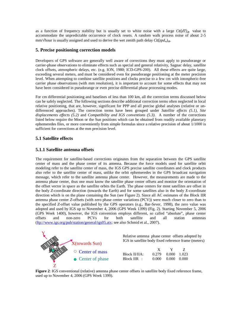
The requirement for satellite-based corrections originates from the separation between the GPS satellitecenter of mass and the phase center of its antenna. Because the force models used for satellite orbitmodeling refer to the satellite center of mass, the IGS GPS precise satellite coordinates and clock productsalso refer to the satellite center of mass, unlike the orbit ephemeredes in the GPS broadcast navigationmessage, which refer to the satellite antenna phase center. However, the measurements are made to theantenna phase center, thus one must know the satellite phase center offsets and monitor the orientation ofthe offset vector in space as the satellite orbits the Earth. The phase centers for most satellites are offset inthe body Z-coordinate direction (towards the Earth) and for some satellites also in the body X-coordinatedirection which is on the plane containing the Sun (see Figure 2). Since all AC estimates of the Block IIRantenna phase center Z-offsets (with zero phase center variations (PCV)) were much closer to zero than tothe specified Z-offset value published by the GPS operators (e.g., Bar-Sever, 1998), the zero value wasadopted and used by IGS up to November 4, 2006 (GPS Week 1399) (Fig. 2). Starting November 5, 2006(GPS Week 1400), however, the IGS convention employs different, so called “absolute”, phase centeroffsets and non-zero PCVs for both satellite and all station antennas(ftp://www.igs.org/pub/station/general/igs05.atx; see also Schmid et al., 2007).

Z

Y

X(towards Sun)

Center of mass

Center of phase

Relative antenna phase center offsets adopted byIGS in satellite body fixed reference frame (meters)

X Y ZBlock II/IIA: 0.279 0.000 1.023Block IIR : 0.000 0.000 0.000

Figure 2: IGS conventional (relative) antenna phase center offsets in satellite body fixed reference frame,used up to November 4, 2006 (GPS Week 1399).

5.1.2 Phase wind-up

GPS satellites transmit right circularly polarized (RCP) radio waves and therefore, the observed carrier-phase depends on the mutual orientation of the satellite and receiver antennas. A rotation of either receiveror satellite antenna around its bore (vertical) axis will change the carrier-phase up to one cycle (onewavelength), which corresponds to one complete revolution of the antenna. This effect is called “phasewind-up” (Wu et al., 1993). A receiver antenna, unless mobile, does not rotate and remains orientedtowards a fixed reference direction (usually north). However, satellite antennas undergo slow rotations astheir solar panels are being oriented towards the Sun and the station-satellite geometry changes. Further, inorder to reorient their solar panels towards the Sun during eclipsing seasons, satellites are also subjected torapid rotations, so called “noon” (when a straight line, starting from the Sun, intersects the satellite and thenthe center of the Earth) and “midnight turns” (when the line intersects the center of the Earth, then thesatellite). This can represent antenna rotations of up to one revolution within less than half an hour. Duringsuch noon or midnight turns, phase data needs to be corrected for this effect (Bar-Sever, 1996; Kouba2008) or simply edited out.

The phase wind-up correction has been generally neglected even in the most precise differential positioningsoftware, as it is quite negligible for double difference positioning on baselines/networks spanning up to afew hundred kilometers. However, it has been shown to reach up to 4 cm for a baseline of 4000 km (Wu etal., 1993). This effect is significant for un-differenced point positioning when fixing IGS satellite clocks,since it can reach up to one half of the wavelength. Since about 1994, most of the IGS Analysis Centers(and therefore the IGS orbit/clock combined products) apply this phase wind-up correction. Neglecting itand fixing IGS orbits/clocks will result in position and clock errors at the dm level. For receiver antennarotations (e.g. during kinematic positioning/navigation) the phase wind-up is fully absorbed into stationclock solutions (or eliminated by double differencing).

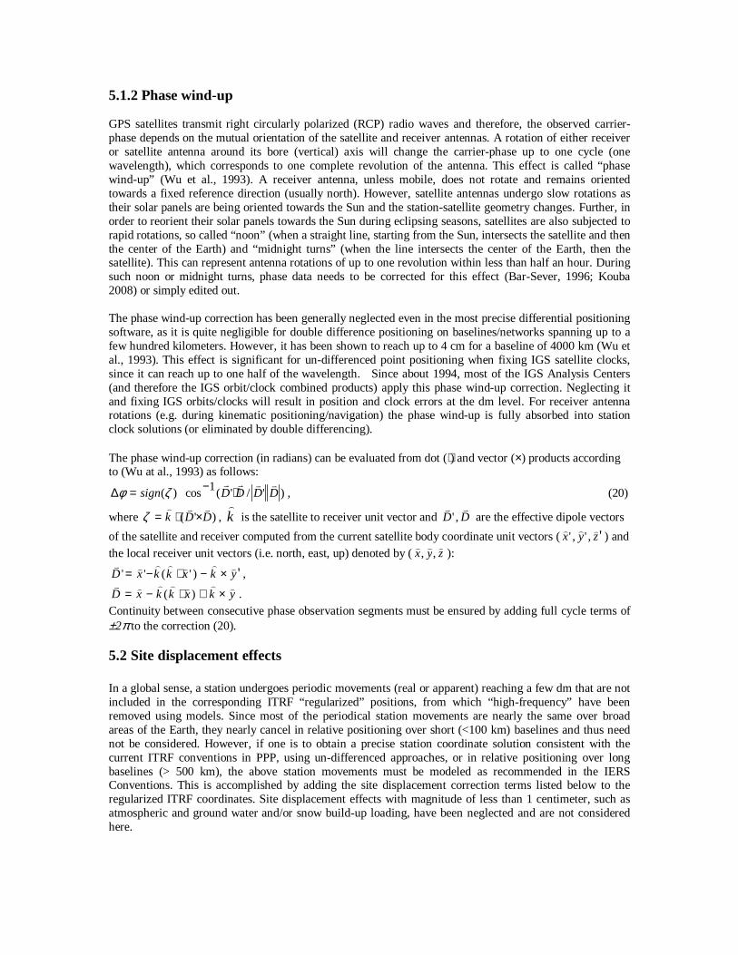
The phase wind-up correction (in radians) can be evaluated from dot (⋅) and vector (×) products accordingto (Wu at al., 1993) as follows:

)'/'(1cos)( DDDDsign����

⋅−=∆ ζφ , (20)

where )'( DDk��⌢

×⋅=ζ , k⌢

is the satellite to receiver unit vector and DD��

,' are the effective dipole vectors

of the satellite and receiver computed from the current satellite body coordinate unit vectors ( ',',' zyx ⌢⌢⌢ ) andthe local receiver unit vectors (i.e. north, east, up) denoted by ( zyx

⌢⌢⌢ ,, ):

')'('' ykxkkxD⌢⌢⌢⌢⌢⌢�

×−⋅−= ,

ykxkkxD⌢⌢⌢⌢⌢⌢�

×+⋅−= )( .Continuity between consecutive phase observation segments must be ensured by adding full cycle terms of±2π to the correction (20).

5.2 Site displacement effects

In a global sense, a station undergoes periodic movements (real or apparent) reaching a few dm that are notincluded in the corresponding ITRF “regularized” positions, from which “high-frequency” have beenremoved using models. Since most of the periodical station movements are nearly the same over broadareas of the Earth, they nearly cancel in relative positioning over short (<100 km) baselines and thus neednot be considered. However, if one is to obtain a precise station coordinate solution consistent with thecurrent ITRF conventions in PPP, using un-differenced approaches, or in relative positioning over longbaselines (> 500 km), the above station movements must be modeled as recommended in the IERSConventions. This is accomplished by adding the site displacement correction terms listed below to theregularized ITRF coordinates. Site displacement effects with magnitude of less than 1 centimeter, such asatmospheric and ground water and/or snow build-up loading, have been neglected and are not consideredhere.

5.2.1 Solid earth tides

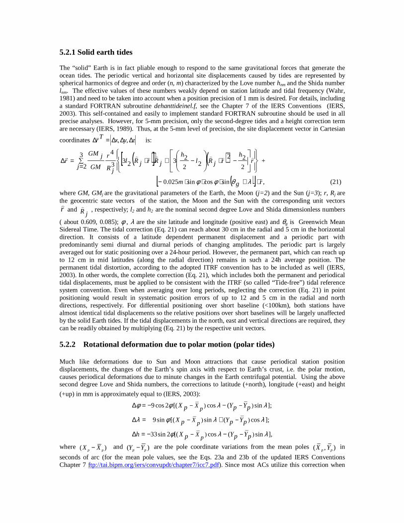
The “solid” Earth is in fact pliable enough to respond to the same gravitational forces that generate theocean tides. The periodic vertical and horizontal site displacements caused by tides are represented byspherical harmonics of degree and order (n, m) characterized by the Love number hnm and the Shida numberlnm. The effective values of these numbers weakly depend on station latitude and tidal frequency (Wahr,1981) and need to be taken into account when a position precision of 1 mm is desired. For details, includinga standard FORTRAN subroutine dehanttideinel.f, see the Chapter 7 of the IERS Conventions (IERS,2003). This self-contained and easily to implement standard FORTRAN subroutine should be used in allprecise analyses. However, for 5-mm precision, only the second-degree tides and a height correction termare necessary (IERS, 1989). Thus, at the 5-mm level of precision, the site displacement vector in Cartesian

coordinates zyxTr ∆∆∆=∆ ,,�

is:

( )[ ] ( )

−⋅−+⋅∑

==∆ r

hrjRl

hjRrjRl

jR

r

j GM

jGMr

⌢⌢⌢⌢⌢⌢�

2

2222

23233

43

2 +

( )[ ] ,sincossin025.0 rgm⌢⋅+⋅⋅⋅− λθφφ (21)

where GM, GMj are the gravitational parameters of the Earth, the Moon (j=2) and the Sun (j=3); r, Rj arethe geocentric state vectors of the station, the Moon and the Sun with the corresponding unit vectorsr⌢

and jR⌢ , respectively; l2 and h2 are the nominal second degree Love and Shida dimensionless numbers

( about 0.609, 0.085); φ , λ are the site latitude and longitude (positive east) and θg is Greenwich MeanSidereal Time. The tidal correction (Eq. 21) can reach about 30 cm in the radial and 5 cm in the horizontaldirection. It consists of a latitude dependent permanent displacement and a periodic part withpredominantly semi diurnal and diurnal periods of changing amplitudes. The periodic part is largelyaveraged out for static positioning over a 24-hour period. However, the permanent part, which can reach upto 12 cm in mid latitudes (along the radial direction) remains in such a 24h average position. Thepermanent tidal distortion, according to the adopted ITRF convention has to be included as well (IERS,2003). In other words, the complete correction (Eq. 21), which includes both the permanent and periodicaltidal displacements, must be applied to be consistent with the ITRF (so called “Tide-free”) tidal referencesystem convention. Even when averaging over long periods, neglecting the correction (Eq. 21) in pointpositioning would result in systematic position errors of up to 12 and 5 cm in the radial and northdirections, respectively. For differential positioning over short baseline (<100km), both stations havealmost identical tidal displacements so the relative positions over short baselines will be largely unaffectedby the solid Earth tides. If the tidal displacements in the north, east and vertical directions are required, theycan be readily obtained by multiplying (Eq. 21) by the respective unit vectors.

5.2.2 Rotational deformation due to polar motion (polar tides)

Much like deformations due to Sun and Moon attractions that cause periodical station positiondisplacements, the changes of the Earth’s spin axis with respect to Earth’s crust, i.e. the polar motion,causes periodical deformations due to minute changes in the Earth centrifugal potential. Using the abovesecond degree Love and Shida numbers, the corrections to latitude (+north), longitude (+east) and height

(+up) in mm is approximately equal to (IERS, 2003):

) )

) )

) )

9 cos 2 [( cos ( sin ];

9sin [( sin ( cos ];

33sin 2 [( cos ( sin ],

X p

X p

X p

X Y Yp p p

X Y Yp p p

h X Y Yp p p

φ φ λ λ

λ φ λ λ

φ λ λ

− −

− −

− −

∆ = − −

∆ = +

∆ = − −

where ( )p pX X− and ( )p pY Y− are the pole coordinate variations from the mean poles ( , )p pX Y in

seconds of arc (for the mean pole values, see the Eqs. 23a and 23b of the updated IERS ConventionsChapter 7 ftp://tai.bipm.org/iers/convupdt/chapter7/icc7.pdf). Since most ACs utilize this correction when

generating their orbit/clock solutions, the IGS combined orbits/clocks are consistent with these stationposition corrections. In other words, for sub-centimeter position precision the above polar tide correctionsneed to be applied to obtain an apparent station position, that is the above corrections have to be subtractedfrom the position solutions in order to be consistent with ITRF. Unlike the solid earth tides (Section 5.2.1)and the ocean loading effects (see Section 5.2.3 below) the pole tides do not average to nearly zero over a24h period. As seen above they are slowly changing according to the polar motion, i.e. they havepredominately seasonal and Chandler (~430 day) periods. Since the polar motion can reach up to 0.8 arcsec, the maximum polar tide displacements can reach about 25 mm in the height and about 7 mm in thehorizontal directions.

5.2.3 Ocean loading

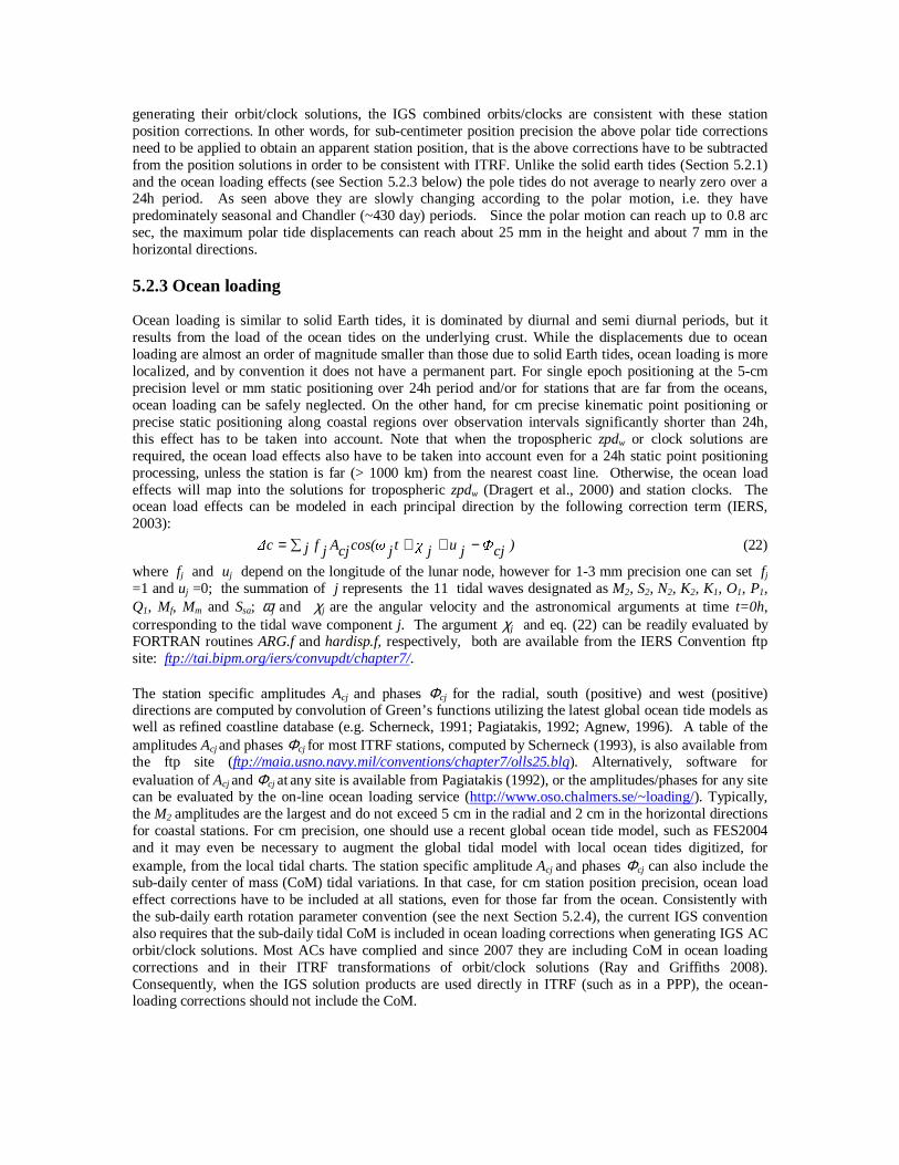
Ocean loading is similar to solid Earth tides, it is dominated by diurnal and semi diurnal periods, but itresults from the load of the ocean tides on the underlying crust. While the displacements due to oceanloading are almost an order of magnitude smaller than those due to solid Earth tides, ocean loading is morelocalized, and by convention it does not have a permanent part. For single epoch positioning at the 5-cmprecision level or mm static positioning over 24h period and/or for stations that are far from the oceans,ocean loading can be safely neglected. On the other hand, for cm precise kinematic point positioning orprecise static positioning along coastal regions over observation intervals significantly shorter than 24h,this effect has to be taken into account. Note that when the tropospheric zpdw or clock solutions arerequired, the ocean load effects also have to be taken into account even for a 24h static point positioningprocessing, unless the station is far (> 1000 km) from the nearest coast line. Otherwise, the ocean loadeffects will map into the solutions for tropospheric zpdw (Dragert et al., 2000) and station clocks. Theocean load effects can be modeled in each principal direction by the following correction term (IERS,2003):

)cj�

juj�tjcos(�cjAj jf

�c −++∑= (22)

where fj and uj depend on the longitude of the lunar node, however for 1-3 mm precision one can set fj=1 and uj =0; the summation of j represents the 11 tidal waves designated as M2, S2, N2, K2, K1, O1, P1,Q1, Mf, Mm and Ssa; ωj and χj are the angular velocity and the astronomical arguments at time t=0h,corresponding to the tidal wave component j. The argument χj and eq. (22) can be readily evaluated byFORTRAN routines ARG.f and hardisp.f, respectively, both are available from the IERS Convention ftpsite: ftp://tai.bipm.org/iers/convupdt/chapter7/.

The station specific amplitudes Acj and phases Φcj for the radial, south (positive) and west (positive)directions are computed by convolution of Green’s functions utilizing the latest global ocean tide models aswell as refined coastline database (e.g. Scherneck, 1991; Pagiatakis, 1992; Agnew, 1996). A table of theamplitudes Acj and phases Φcj for most ITRF stations, computed by Scherneck (1993), is also available fromthe ftp site (ftp://maia.usno.navy.mil/conventions/chapter7/olls25.blq). Alternatively, software forevaluation of Acj and Φcj at any site is available from Pagiatakis (1992), or the amplitudes/phases for any sitecan be evaluated by the on-line ocean loading service (http://www.oso.chalmers.se/~loading/). Typically,the M2 amplitudes are the largest and do not exceed 5 cm in the radial and 2 cm in the horizontal directionsfor coastal stations. For cm precision, one should use a recent global ocean tide model, such as FES2004and it may even be necessary to augment the global tidal model with local ocean tides digitized, forexample, from the local tidal charts. The station specific amplitude Acj and phases Φcj can also include thesub-daily center of mass (CoM) tidal variations. In that case, for cm station position precision, ocean loadeffect corrections have to be included at all stations, even for those far from the ocean. Consistently withthe sub-daily earth rotation parameter convention (see the next Section 5.2.4), the current IGS conventionalso requires that the sub-daily tidal CoM is included in ocean loading corrections when generating IGS ACorbit/clock solutions. Most ACs have complied and since 2007 they are including CoM in ocean loadingcorrections and in their ITRF transformations of orbit/clock solutions (Ray and Griffiths 2008).Consequently, when the IGS solution products are used directly in ITRF (such as in a PPP), the ocean-loading corrections should not include the CoM.

5.2.4 Earth rotation parameters (ERP)

The Earth Rotation Parameters (i.e. pole position Xp, Yp and UT1-UTC), along with the conventions forsidereal time, precession and nutation facilitate accurate transformations between terrestrial and inertialreference frames that are required in global GPS analysis (see e.g. IERS, 2003). Then, the resulting orbitsin the terrestrial conventional reference frame (ITRF), much like the IGS orbit products, imply, quiteprecisely, the underlying ERP. Consequently, IGS users who fix or heavily constrain the IGS orbits andwork directly in ITRF need not worry about ERP. However, when using software formulated in an inertialframe, the ERP, corresponding to the fixed orbits, augmented with the so called sub-daily ERP model, arerequired and must be used. This is so, since ERP, according to the IERS convention are regularized and donot include the sub-daily, tidally induced, ERP variations.

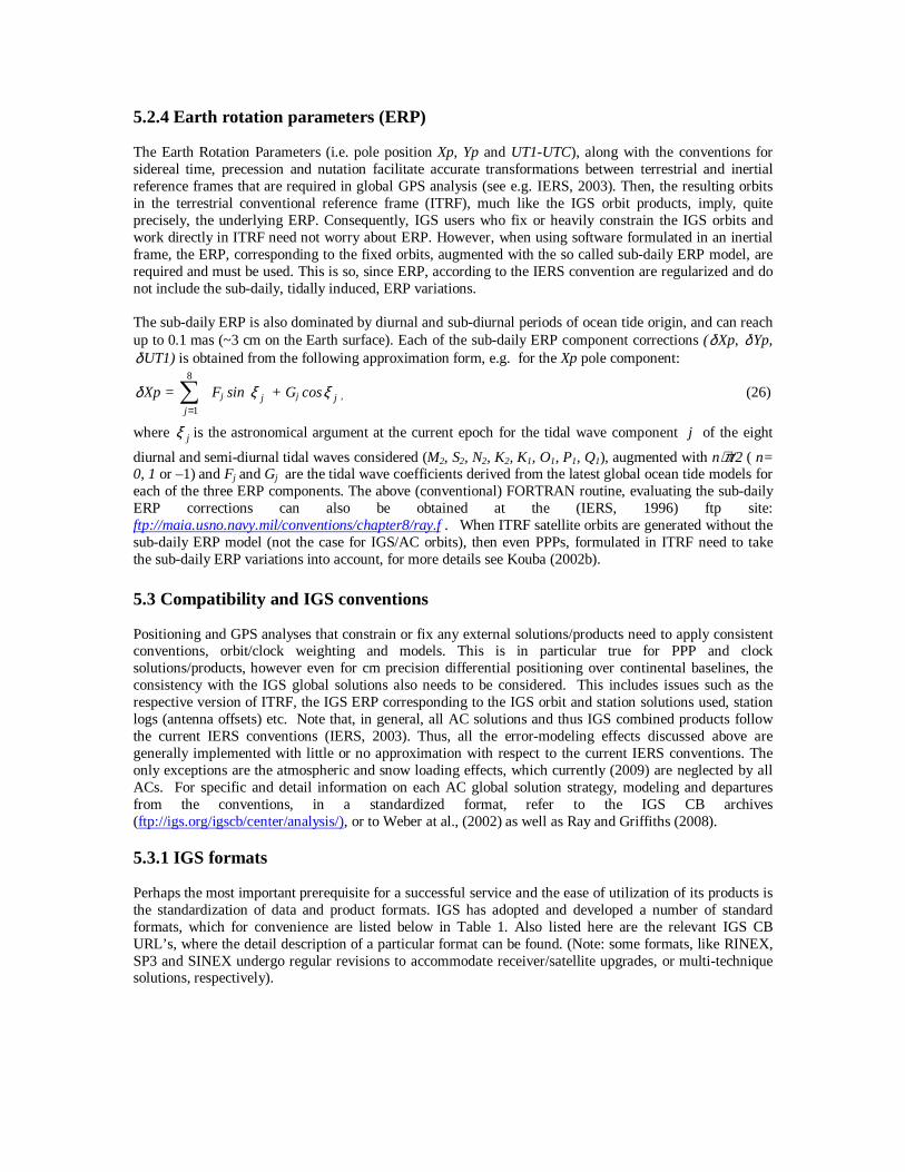
The sub-daily ERP is also dominated by diurnal and sub-diurnal periods of ocean tide origin, and can reachup to 0.1 mas (~3 cm on the Earth surface). Each of the sub-daily ERP component corrections (δXp, δYp,δUT1) is obtained from the following approximation form, e.g. for the Xp pole component:

δXp = ∑=

8

1j

Fj sin jξ + Gj cos jξ , (26)

where jξ is the astronomical argument at the current epoch for the tidal wave component j of the eight

diurnal and semi-diurnal tidal waves considered (M2, S2, N2, K2, K1, O1, P1, Q1), augmented with n⋅π/2 ( n=0, 1 or –1) and Fj and Gj are the tidal wave coefficients derived from the latest global ocean tide models foreach of the three ERP components. The above (conventional) FORTRAN routine, evaluating the sub-dailyERP corrections can also be obtained at the (IERS, 1996) ftp site:ftp://maia.usno.navy.mil/conventions/chapter8/ray.f . When ITRF satellite orbits are generated without thesub-daily ERP model (not the case for IGS/AC orbits), then even PPPs, formulated in ITRF need to takethe sub-daily ERP variations into account, for more details see Kouba (2002b).

5.3 Compatibility and IGS conventions

Positioning and GPS analyses that constrain or fix any external solutions/products need to apply consistentconventions, orbit/clock weighting and models. This is in particular true for PPP and clocksolutions/products, however even for cm precision differential positioning over continental baselines, theconsistency with the IGS global solutions also needs to be considered. This includes issues such as therespective version of ITRF, the IGS ERP corresponding to the IGS orbit and station solutions used, stationlogs (antenna offsets) etc. Note that, in general, all AC solutions and thus IGS combined products followthe current IERS conventions (IERS, 2003). Thus, all the error-modeling effects discussed above aregenerally implemented with little or no approximation with respect to the current IERS conventions. Theonly exceptions are the atmospheric and snow loading effects, which currently (2009) are neglected by allACs. For specific and detail information on each AC global solution strategy, modeling and departuresfrom the conventions, in a standardized format, refer to the IGS CB archives(ftp://igs.org/igscb/center/analysis/), or to Weber at al., (2002) as well as Ray and Griffiths (2008).

5.3.1 IGS formats

Perhaps the most important prerequisite for a successful service and the ease of utilization of its products isthe standardization of data and product formats. IGS has adopted and developed a number of standardformats, which for convenience are listed below in Table 1. Also listed here are the relevant IGS CBURL’s, where the detail description of a particular format can be found. (Note: some formats, like RINEX,SP3 and SINEX undergo regular revisions to accommodate receiver/satellite upgrades, or multi-techniquesolutions, respectively).

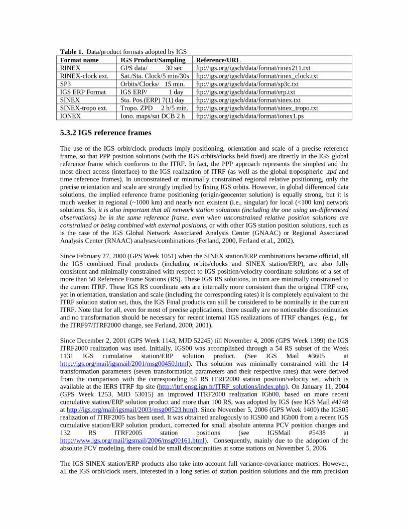
Table 1. Data/product formats adopted by IGSFormat name IGS Product/Sampling Reference/URLRINEX GPS data/ 30 sec ftp://igs.org/igscb/data/format/rinex211.txtRINEX-clock ext. Sat./Sta. Clock/5 min/30s ftp://igs.org/igscb/data/format/rinex_clock.txtSP3 Orbits/Clocks/ 15 min. ftp://igs.org/igscb/data/format/sp3c.txtIGS ERP Format IGS ERP/ 1 day ftp://igs.org/igscb/data/format/erp.txtSINEX Sta. Pos.(ERP) 7(1) day ftp://igs.org/igscb/data/format/sinex.txtSINEX-tropo ext. Tropo. ZPD 2 h/5 min. ftp://igs.org/igscb/data/format/sinex_tropo.txtIONEX Iono. maps/sat DCB 2 h ftp://igs.org/igscb/data/format/ionex1.ps

5.3.2 IGS reference frames

The use of the IGS orbit/clock products imply positioning, orientation and scale of a precise referenceframe, so that PPP position solutions (with the IGS orbits/clocks held fixed) are directly in the IGS globalreference frame which conforms to the ITRF. In fact, the PPP approach represents the simplest and themost direct access (interface) to the IGS realization of ITRF (as well as the global tropospheric zpd andtime reference frames). In unconstrained or minimally constrained regional relative positioning, only theprecise orientation and scale are strongly implied by fixing IGS orbits. However, in global differenced datasolutions, the implied reference frame positioning (origin/geocenter solution) is equally strong, but it ismuch weaker in regional (~1000 km) and nearly non existent (i.e., singular) for local (<100 km) networksolutions. So, it is also important that all network station solutions (including the one using un-differencedobservations) be in the same reference frame, even when unconstrained relative position solutions areconstrained or being combined with external positions, or with other IGS station position solutions, such asis the case of the IGS Global Network Associated Analysis Center (GNAAC) or Regional AssociatedAnalysis Center (RNAAC) analyses/combinations (Ferland, 2000, Ferland et al., 2002).

Since February 27, 2000 (GPS Week 1051) when the SINEX station/ERP combinations became official, allthe IGS combined Final products (including orbits/clocks and SINEX station/ERP), are also fullyconsistent and minimally constrained with respect to IGS position/velocity coordinate solutions of a set ofmore than 50 Reference Frame Stations (RS). These IGS RS solutions, in turn are minimally constrained tothe current ITRF. These IGS RS coordinate sets are internally more consistent than the original ITRF one,yet in orientation, translation and scale (including the corresponding rates) it is completely equivalent to theITRF solution station set, thus, the IGS Final products can still be considered to be nominally in the currentITRF. Note that for all, even for most of precise applications, there usually are no noticeable discontinuitiesand no transformation should be necessary for recent internal IGS realizations of ITRF changes. (e.g., forthe ITRF97/ITRF2000 change, see Ferland, 2000; 2001).

Since December 2, 2001 (GPS Week 1143, MJD 52245) till November 4, 2006 (GPS Week 1399) the IGSITRF2000 realization was used. Initially, IGS00 was accomplished through a 54 RS subset of the Week1131 IGS cumulative station/ERP solution product. (See IGS Mail #3605 athttp://igs.org/mail/igsmail/2001/msg00450.html). This solution was minimally constrained with the 14transformation parameters (seven transformation parameters and their respective rates) that were derivedfrom the comparison with the corresponding 54 RS ITRF2000 station position/velocity set, which isavailable at the IERS ITRF ftp site (http://itrf.ensg.ign.fr/ITRF_solutions/index.php). On January 11, 2004(GPS Week 1253, MJD 53015) an improved ITRF2000 realization IGb00, based on more recentcumulative station/ERP solution product and more than 100 RS, was adopted by IGS (see IGS Mail #4748at http://igs.org/mail/igsmail/2003/msg00523.html). Since November 5, 2006 (GPS Week 1400) the IGS05realization of ITRF2005 has been used. It was obtained analogously to IGS00 and IGb00 from a recent IGScumulative station/ERP solution product, corrected for small absolute antenna PCV position changes and132 RS ITRF2005 station positions (see IGSMail #5438 athttp://www.igs.org/mail/igsmail/2006/msg00161.html). Consequently, mainly due to the adoption of theabsolute PCV modeling, there could be small discontinuities at some stations on November 5, 2006.

The IGS SINEX station/ERP products also take into account full variance-covariance matrices. However,all the IGS orbit/clock users, interested in a long series of station position solutions and the mm precision

level, still need to take into account all the ITRF changes. This is particularly true for PPP and global orcontinental relative station positioning. More specifically, since its beginning in 1994, IGS has used sevendifferent, official realizations of ITRF (ITRF92, ITRF93, ITRF94, ITRF96, ITRF97, ITRF2000 andITRF2005). The exact dates of the ITRF changes, estimated transformation parameters and a simpleFortran 77 transformation program are available at the following ftp site:ftp://macs.geod.nrcan.gc.ca/pub/requests/itrf96_97 (also see Kouba, 2002a). Most of the ITRF changes areat or below the 10-mm level, with the notable exception of the ITRF92-93 and ITRF93-94 transformations,where rotational changes of more than .001” (30 mm) were introduced due to a convention change in theorientation evolution of ITRF93 (see e.g. Kouba and Popelar, 1994). It is important to note that only theITRF96-97 (on August 1, 1999), ITRF97-2000 (December 2, 2001), ITRF2000-2005 (November 5, 2006)and any future ITRF changes have virtually exact transformations (due to the minimum constraining usedsince 1998). However, all the preceding transformations (i.e. prior the ITRF96-97 change) are onlyapproximate and can be used for transformations at the 1-3 mm (0.0001” for ERP) precision level only. Tominimize any discontinuity as well as to increase precision and consistency of IGS products, during 2008-2009 IGS has undertaken reprocessing all the data prior 2008, possibly up to 1994 (seehttp://acc.igs.org/reprocess.html). By the end of 2009, when the reprocessing is completed and verified, itshould replace all the pre-2008 IGS products (see IGSMAIL #5873 athttp://igs.org/mail/igsmail/2008/msg00195.html). So, a complete and consistent series of IGS combined(weekly) SINEX and (daily) orbit/clock combined solutions in IGS05 and based on the absolute antennaPCVs should be available at the IGS Global Data Centers by 2010.

The ITRF convention allows linear station movements only (apart from the conventionally modeled high-frequency tidal variations), i.e. dated initial station positions and the station velocities, which is notadequate at the mm-level precision, as even stable stations exhibit real and apparent non-linear departuresthat can exceed 10 mm. Often, the station movements are of periodical (e.g. seasonal and semi-seasonal)character. The non-linear station movements can be induced, for example, by various uncorrected loadingeffects (atmospheric, snow), or by the real non-tidal variation of geocenter and scale (i.e. the Earth’sdimension). Currently, a new ITRF convention is being considered, where the long period (>> 1 day)geocenter variations with respect to a conventional ITRF origin would have to be monitored and becomepart of the new ITRF convention (much like ERP monitoring is an integral part of ITRF). This newconvention, after accounting for all the loading effects, should provide an ITRF realization of stable stationpositions at the mm level.

The IGS Rapid products are consistent with the current ITRF convention, i.e. IGS05 positions of the IGSRS stations are fixed in all the IGS AC Rapid solutions, thus no geocenter or scale variations are allowedand none should show up in the solutions when using IGS Rapid/clock products. However, all the IGSFinal solutions and products, mainly to facilitate higher internal precision/consistency, but also inanticipation of the new ITRF convention, since June 28, 1998 are based on minimal rotational constraintsonly. Note that unconstrained global GPS solutions are nearly singular only in orientation, they still containa strong origin (geocenter) and scale information due to orbit dynamics (i.e. the adopted gravity field). So,after June 28, 1998, all the IGS Final orbits/clocks, at least nominally, refer to the real geocenter and scalethat undergo small (~10mm) variations with respect to the adopted ITRF origin and scale. The new ITRFconvention has in fact already been adopted starting with the IGS00 RS station set, as well as for all theIGS weekly (IGSYYPWWWW.snx) and cumulative (IGSYYPWW.snx) SINEX products. Since thegeocenter positions and scale biases are solved for and published every week when the IGS accumulatedproducts are being augmented with the current week (independent from week to week) SINEXcombinations, which contain the weekly mean geocenters. However, currently (2009) the correspondingIGS Final orbit combinations are not corrected for the daily geocenter/scale variation. Even in the new IGSFinal clock combinations, which has become official on November 5, 2000 (IGS Mail #3087) and which, inevery other aspect was made highly consistent with the IGS SINEX/ERP cumulative combinations asoutlined in Kouba et al. (1998) and Kouba and Springer (2000), the geocenter clock corrections were notimplemented. The IGS Final and all AC orbit/clock solutions were not transformed, thus they fullyreflected (i.e. they are with respect to) the apparent or real geocenter/scale variations. However, sinceNovember 5, 2006 AC and IGS clocks are supposed to be transferred to the ITRF origin. Thus all globalanalyses utilizing differenced observations and using only the IGS Final orbits (unlike the IGS Rapidorbits) still have to take into consideration the small (~10 mm) weekly geocenter and scale variations as the

geocenter/scale variations are fully implied by the IGS Final orbits. On the other hand, regional relativepositioning with fixed IGS Final orbits and from November 5, 2006 PPP’s with the IGS Final orbit/clockproducts held fixed, should show only small weekly scale (height) variations. This is so, since relativeregional analyses are less sensitive to orbit origin and in case of PPP, the apparent geocenter variationshould be properly accounted for in the current IGS Final clock combinations. Thus, since November 5,2006, the IGS Final orbit/clock PPP users will only have to consider (with respect to IGS05 (ITRF2005))small (~cm) weekly scale (height) biases, which are not yet accounted for in the new, now official, IGSFinal orbit/clock combinations.

In summary, all (global) applications involving IGR rapid orbit/clock products should be directly in theconventional ITRF and no origin/scale variations should be seen. On the other hand, all global applicationsusing (i.e. fixing) the IGS Final orbit products will refer to a mean geocenter and scale of the week, thussmall (weekly) variations in origin/scale with respect to ITRF could be seen. After November 5, 2006 allPPP solutions based on the IGS Final products should show only small weekly scale (height) variations,since IGS Final orbit origin variations should be accounted for in the current Final clock combinations. Atthe precision level of about 10-mm, when using the IGS Final products, all the above origin/scale variationscan likely be neglected. The above small weekly IGS geocenter (origin) variation can be found in thecorresponding GPS week (WWWW) SINEX combinations and summary files (IGSYYPWWWW.sum),which are also available at the IGS CB (http://www.igs.org/mail/igsreport/igsreport.html). Perhaps, a moreacceptable and consistent approach would be also to remove, if possible, from the IGS Final combinedorbit products all the origin/scale variations with respect to the adopted ITRF. This has already beensuggested in Kouba and Springer (2000).

5.3.3 IGS receiver antenna phase center offsets/tables

Prior to November 5, 2006, unless using Dorne-Margolin (D/M) antennas, the relative IGS antenna PCVtable (igs_01.pcv) that are available at the IGS Central Bureau (ftp://www.igs.org/pub/station/general/) andthe conventional satellite antenna offset of Fig.2 should be used with the IGS solution products. AfterNovember 5, 2006, (and/or for any reprocessed IGS orbits/clocks) the absolute receiver and satelliteantenna PCV and offsets of the current igs05.atx file should be used. If a receiver antenna type is notcontained in the current igs05.atx, the satellite antenna offsets of Fig.2 and the zero or relative PCV/offsets(igs_01.pcv ) should be used for the receiver antenna. The relative and absolute satellite and receiverantenna PCVs and offsets should never be mixed, as such an inconsistent use of satellite/receiver PCVs andoffsets will result in position biases (mainly in height) up to 10 cm. Note that when the relative PCVs andoffsets (igs_01.pcv) are used for receiver antennas together with the satellite antenna offsets of Fig. 2,acceptable results are still obtained even when the orbits/clocks were generated with the absolute satelliteantenna PCVs and offsets.

For precise relative positioning with different antenna types even over short baselines, and in particularwhen solving for tropospheric zpd’s, the IGS antenna PCV tables (either absolute or relative) are alsomandatory, otherwise, large errors up to 10 cm in height and zpdw solutions may result. On the other hand,relative positioning with the same antenna type over short to medium length baselines (<1000 km), with orwithout the zpdw solutions does not require the use of the antenna PCV. Since PPP is in fact equivalent to astation position solution within a global (IGS) network solutions (but conveniently condensed within theIGS precise orbit/clock products), it must always use the appropriate IGS antenna PCV to ensurecompatibility with the IGS antenna PCV convention. Before November 5, 2006, the IGS antenna PCVtable (igs_01.pcv) was relative to the D/M antenna type, thus the IGS orbit/clock products were consistentwith the D/M antennas and all the PPP’s involving D/M antennas could safely neglect the igs_01.pcv table.However, for best results, after November 5, 2006 and/or for the reprocessed IGS products, every PPP,even with D/M antennas, should use for both receiver and satellite antennas, specific (absolute) antennaPCV tables, adopted by IGS (igs05.atx). Note that even if no PCV tables are necessary (e.g. for cm relativepositioning with no zpdw solutions), the constant receiver antenna height offsets, given in the igs_01.pcvtable, along with the offsets of Fig.2, are still mandatory in this case. The absolute satellite antenna PCVs(e.g., igs05.atx) have nearly eliminated the apparent station scale bias of about 15 ppb, seen in globalunconstrained GPS station/orbit solutions when absolute receiver antenna PCVs and the (relative) satellite

antenna offsets of Fig. 2 were used (see e.g. Rothacher et al., 1995; Springer, 1999; Rothacher and Mader,2002).

5.3.4 Modeling/observation conventions

The GPS System already has some well developed modeling conventions, e.g., that only the periodicrelativity correction

2/2 csVsXrelt��

⋅−=∆ (27)

is to be applied by all GPS users (ION, 1980; ICD-GPS-200, 1991). Here sVsX��

, are the satellite positionand velocity vectors and c is the speed of light. The same convention has also been adopted by IGS, i.e., allthe IGS satellite clock solutions are consistent with and require this correction. Approximation errors ofthis standard GPS relativity treatment are well below the 0.1 ns and 10-14 level for time and frequency,respectively (e.g. Kouba, 2002c; 2004).

By an agreed convention, there are no L1-L2 (or P1-P2) Differential Calibration Bias (DCB) correctionsapplied in all the IGS AC analyses, thus no such DCB calibrations are to be applied when the IGS clockproducts are held fixed or constrained in dual frequency PPP or time transfers. Furthermore, a specific setof pseudorange observations, consistent with the IGS clock products, needs to be used, otherwise thestation clock and position solutions would be degraded. This is a result of significant satellite dependentdifferences between C/A (C1) and P1 code pseudoranges, which can reach up to 2 ns (60 cm). Note thatIGS has been using the following conventional pseudorange observation sets, which needs to be used withthe IGS orbit/clock products (IGS Mail #2744):

PC/A and P’2 = PC/A + (P2-P1) Up to April 02, 2000 (GPS Week 1056),P1 and P2 After April 02, 2000 (GPS Week 1056).

For C/A and P–code carrier phase observations (LC/A and LP1) there is no such problem and no need for anysuch convention, since according to the GPS system specifications (ICD-GPS200, 1991, p.11) thedifference between the two types of L1 phase observations is the same for all satellites and it is equal to aquarter of the L1 wavelength. This phase difference is then fully absorbed by the initial real phaseambiguities. However, early on, most receiver manufactures have agreed to align LC/A and LP1 phaseobservations (J. Ray, person. comm. 2009). For more information on this pseudorange observationconvention and how to form the conventional pseudorange observation set for receivers, which do not giveall the necessary pseudorange observations, see the IGS Mail #2744 at(http://www.igs.org/mail/igsmail/2000/maillist.html).

6. Single-frequency positioning

Precise, i.e., mm-level, positioning with single-frequency and without any external ionospheric delaycorrections, is only possible for relative positioning over very short (<10 km) baselines. For such shortbaselines using IGS precise orbits offers little or no benefit over the broadcast orbits. With ionosphericdelay corrections, derived, for example, from the IGS ionospheric grid maps generated by the IGSIonospheric Working Group (http://www.igs.org/projects/iono/index.html) relative single-frequency cm-positioning could be extended up to a few hundred km when using the IGS precise orbits. Here the IGSprecise orbits already could offer some accuracy improvements over the broadcast orbits.

Single-frequency PPP must also use the above-derived ionospheric delay corrections along with thecorresponding satellite (L1-L2) Differential Calibration Delays (DCB); even then only precision at aboutthe 0.5 m level is possible with the IGS orbits/clocks, which is mainly due to a limited resolution andprecision of the IGS ionospheric grid maps. Neglecting the satellite (L1-L2) DCB’s, which are nearlyconstant in time, but vary from satellite to satellite and can reach up to 12 ns, (i.e., using only theionospheric delay corrections), would result in significant positioning errors that may be even larger(several meters) than the errors of uncorrected, single-frequency PPP solutions (Heroux, 1993, personalcom.). This is so, since the IGS clocks are consistent with the (L1-L2) DCB convention (this is also true for

the GPS broadcast clocks), i.e. the single-frequency IGS users have to first correct the IGS satellite clocksby -1.55 (L1-L2) DCB, (28)in order to make them compatible with the single-frequency observations. (Note the different signconvention for the broadcast (L1-L2) group delays TGD, which after April 29, 1999 are quite precise and canalso be used even in the most precise applications (http://www.igs.org/mail/igsmail/1999/msg00195.html).For static single-frequency PPP at this precision level, the IGS precise orbits/clocks offer only marginalimprovements with respect to the broadcast orbits and clocks, in particularly with SA switched off (i.e.,after May 02, 2000). However, before May 02, 2000 with SA switched on, a single-frequency static orkinematic (navigation) PPP, with the IGS precise orbits and clocks could offer about an order of magnitudeprecision improvements over the broadcast orbits and clocks. A more precise alternative to single-frequency PPP is to use the ambiguous ionspheric-free combination of (L1+P1)/2 and the P1 (with

appropriately large noise) in place of φℓ (L3) and Pℓ (P3) in a “regular” PPP (Eqs. 7 - 8). Here, C/A (C1)

pseudoranges can be used in place of P1, too. This single-frequency PPP usually yields dm precision andthanks to the ambiguity solutions, it is also less sensitive to any inconsistency (or even neglect) of (C1-P1),(L1-L2) DCBs, as well as satellite antenna PCVs/offsets.

7. Solution precision/accuracy with IGS Combined Products

Accuracy is an elusive word and it is difficult to quantify. In this context, by accuracy here it is meant themeasure of a solution uncertainty with respect to a global, internationally adopted, conventional referenceframe or system. Precision, on the other hand, is much easier to understand and attainable and here it canbe interpreted as solution repeatability within a limited area and over a limited period of time. So, in thisway, precise solutions may be biased and therefore may not be accurate. Formal solutions sigmas (standarddeviations) are most often representative of solution precision rather than accuracy. For IGS users, theaccuracy is perhaps the most important factor, though for some applications, precision may be equally oreven more important, e.g. for crustal deformation or relative movement studies during short periods oftime. It is also important to note that the precision/accuracy of IGS combined products is not constant andthat it has been improving steadily (see Fig. 1) due to both better data quality and quantity (coverage) aswell as significant analysis improvements realized by all ACs.

7.1 Positioning

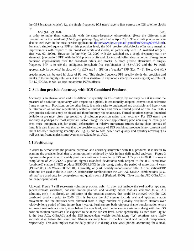
In order to demonstrate the possible precision and accuracy achievable with IGS products, it is useful toexamine the precision level that is being routinely achieved by ACs in their daily global analyses. Figure 3represents the precision of weekly position solutions achievable by IGS and ACs prior to 2000. It shows acompilation of AC/GNAAC position sigmas (standard deviations) with respect to the IGS cumulative(combined) station SINEX product (IGS00P39.SNX in this case), during the period of more than 4 years(1996-2000; GPS Weeks 0837-1081). Currently, only AC weekly unconstrained SINEX final station/ERPsolutions are used in the IGS SINEX station/ERP combinations; the GNAAC SINEX combinations (JPL,mit, ncl) are used only for comparisons and quality control (Ferland, 2000). (Note that the JPL GNAAC isno longer operational)

Although Figure 3 still represents solution precision only, (it does not include the real and/or apparentgeocenter/scale variations, constant station position and velocity biases that are common to all ACsolutions, etc.), it is already an indication of the position accuracy that could be achieved with the IGScombined products prior to 2000. This is because the AC sigmas include real and apparent stationmovements and the statistics were obtained from a large number of globally distributed stations overrelatively long period of time (more than 4 years). Furthermore, both reference frame transformation errorsand mean residuals are small, at or below the mm level, and the geocenter variations along with the IGSposition solution biases are also expected to be at the sub-cm level. More specifically, as seen from Figure3, the best ACs, GNAACs and the IGS independent weekly combinations (igs) solutions were likelyaccurate at or below the 5-mm and 10-mm accuracy level in the horizontal and vertical components,respectively. This also implies that the daily static PPP during a one-week period, accounting for a small

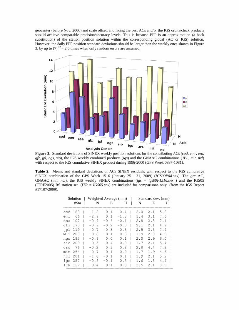
geocenter (before Nov. 2006) and scale offset, and fixing the best ACs and/or the IGS orbits/clock productsshould achieve comparable precision/accuracy levels. This is because PPP is an approximation (a backsubstitution) of the station position solution within the corresponding global (AC or IGS) solution.However, the daily PPP position standard deviations should be larger than the weekly ones shown in Figure3, by up to (7)1/2 = 2.6 times when only random errors are assumed.

cod emr esa gfz jpl ngs sio igs JPL mit ncl

N

H

0

2

4

6

8

10

12

14

Sta

nd

ard

Dev

iati

on

(m

m)

Analysis Center

Axis

w.r.t. the Cumulative Solution

N

E

H

Figure 3. Standard deviations of SINEX weekly position solutions for the contributing ACs (cod, emr, esa,gfz, jpl, ngs, sio), the IGS weekly combined products (igs) and the GNAAC combinations (JPL, mit, ncl)with respect to the IGS cumulative SINEX product during 1996-2000 (GPS Week 0837-1081).

Table 2. Means and standard deviations of ACs SINEX residuals with respect to the IGS cumulativeSINEX combination of the GPS Week 1516 (January 25 - 31, 2009) (IGS09P04.snx). The grc AC,GNAAC (mit, ncl), the IGS weekly SINEX combinations (igs = igs09P1516.snx ) and the IGS05(ITRF2005) RS station set (ITR = IGS05.snx) are included for comparisons only (from the IGS Report#17107/2009).

Solution | Weighted Average (mm) | Standard dev. (mm) | #Sta | N E U | N E U |

----------------------------------------------------------------------------------cod 183 | -1.2 -0.1 -0.4 | 2.0 2.1 5.8 |emr 66 | -2.9 0.1 -1.8 | 3.4 3.1 7.6 |esa 107 | -0.9 -0.6 -0.1 | 2.8 2.5 7.1 |gfz 175 | -0.9 -0.2 -0.3 | 2.1 2.1 4.9 |jpl 119 | -0.7 -0.3 -0.3 | 2.5 3.5 7.4 |MIT 203 | -0.8 -0.1 -0.3 | 1.9 2.0 4.9 |ngs 183 | -0.9 0.0 0.1 | 2.0 2.9 6.0 |sio 209 | 0.5 -0.4 0.0 | 1.7 2.4 5.4 |grg 76 | -0.2 0.3 0.8 | 2.8 4.4 7.8 |mit 254 | -0.7 -0.1 0.0 | 1.7 1.9 4.6 |ncl 201 | -1.0 -0.1 0.1 | 1.9 2.1 5.2 |igs 257 | -0.8 -0.1 0.3 | 1.6 1.8 4.4 |ITR 127 | -0.4 -0.1 0.0 | 2.5 2.4 8.9 |

------------------------------------------------------------------------------------------------------------------------------

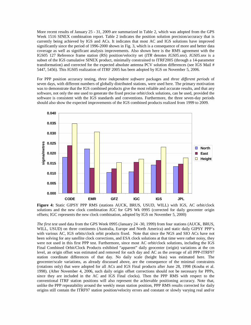
More recent results of January 25 - 31, 2009 are summarized in Table 2, which was adopted from the GPSWeek 1516 SINEX combination report. Table 2 indicates the position solution precision/accuracy that iscurrently being achieved by IGS and ACs. It indicates that most AC and IGS solutions have improvedsignificantly since the period of 1996-2000 shown in Fig. 3, which is a consequence of more and better datacoverage as well as significant analysis improvements. Also shown here is the RMS agreement with theIGS05 127 Reference frame station (RS) position/velocity set (ITR denotes IGS05.snx). IGS05.snx is asubset of the IGS cumulative SINEX product, minimally constrained to ITRF2005 (through a 14-parametertransformation) and corrected for the expected absolute antenna PCV solution differences (see IGS Mail #5447, 5456). This IGS05 realization of ITRF 2005 has been adopted by IGS on November 5, 2006.

For PPP position accuracy testing, three independent software packages and three different periods ofseven days, with different numbers of globally distributed stations, were used here. The primary motivationwas to demonstrate that the IGS combined products give the most reliable and accurate results, and that anysoftware, not only the one used to generate the fixed precise orbit/clock solutions, can be used, provided thesoftware is consistent with the IGS standards and conventions. Furthermore, the three seven-day periodsshould also show the expected improvements of the IGS combined products realized from 1999 to 2009.

0.000

0.005

0.010

0.015

0.020

0.025

0.030

0.035

0.040

CODE EMR GFZ IGC IGS JPL

sig

ma/

met

res

North East Height

Figure 4: Static GIPSY PPP RMS (stations AUCK, BRUS, USUD, WILL) with IGS, AC orbit/clocksolutions and the new clock combination IGC for GPS Wk 0995 (corrected for daily geocenter originoffsets; IGC represents the new clock combination, adopted by IGS on November 5, 2000)

The first test used data from the GPS Week 0995 (January 24 -30, 1999) from four stations (AUCK, BRUS,WILL, USUD) on three continents (Australia, Europe and North America) and static daily GIPSY PPP’swith various AC, IGS orbits/clock orbit products fixed. Note that since the NGS and SIO ACs have notbeen solving for any satellite clock corrections, and ESA clock solutions at that time were rather noisy, theywere not used in this first PPP test. Furthermore, since most AC orbit/clock solutions, including the IGSFinal Combined Orbit/Clock Products exhibited “apparent” daily geocenter (origin) variations at the cmlevel, an origin offset was estimated and removed for each day and AC as the average of all PPP-ITRF97station coordinate differences of that day. No daily scale (height bias) was estimated here. Thegeocenter/scale variations, as already discussed above, are the consequence of the minimal constraints(rotations only) that were adopted for all ACs and IGS Final products after June 28, 1998 (Kouba et al.1998). (After November 4, 2006, such daily origin offset corrections should not be necessary for PPPs,since they are included in the AC and IGS Final clocks). Then the PPP RMS with respect to theconventional ITRF station positions will also represent the achievable positioning accuracy. Note that,unlike the PPP repeatability around the weekly mean station position, PPP RMS results corrected for dailyorigins still contain the ITRF97 station position/velocity errors and constant or slowly varying real and/or

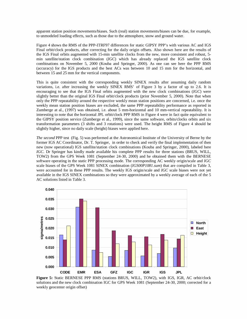
apparent station position movements/biases. Such (real) station movements/biases can be due, for example,to unmodeled loading effects, such as those due to the atmosphere, snow and ground water.

Figure 4 shows the RMS of the PPP-ITRF97 differences for static GIPSY PPP’s with various AC and IGSFinal orbit/clock products, after correcting for the daily origin offsets. Also shown here are the results ofthe IGS Final orbits augmented with 15-min satellite clocks from the new, more consistent and robust, 5-min satellite/station clock combination (IGC) which has already replaced the IGS satellite clockcombinations on November 5, 2000 (Kouba and Springer, 2000). As one can see here the PPP RMS(accuracy) for the IGS products and the best ACs was between 10 and 15 mm for the horizontal, andbetween 15 and 25 mm for the vertical components.

This is quite consistent with the corresponding weekly SINEX results after assuming daily randomvariations, i.e. after increasing the weekly SINEX RMS’ of Figure 3 by a factor of up to 2.6. It isencouraging to see that the IGS Final orbits augmented with the new clock combinations (IGC) wereslightly better than the original IGS Final orbit/clock products (prior November 5, 2000). Note that whenonly the PPP repeatability around the respective weekly mean station positions are concerned, i.e. once theweekly mean station position biases are excluded, the same PPP repeatability performance as reported inZumberge at al., (1997) was obtained, i.e. about 5 mm-horizontal and 10 mm-vertical repeatability. It isinteresting to note that the horizontal JPL orbit/clock PPP RMS in Figure 4 were in fact quite equivalent tothe GIPSY position service (Zumberge et al., 1999), since the same software, orbits/clocks orbits and sixtransformation parameters (3 shifts and 3 rotations) were used. The height RMS of Figure 4 should beslightly higher, since no daily scale (height) biases were applied here.

The second PPP test (Fig. 5) was performed at the Astronomical Institute of the University of Berne by theformer IGS AC Coordinator, Dr. T. Springer, in order to check and verify the final implementation of thennew (now operational) IGS satellite/station clock combinations (Kouba and Springer, 2000), labeled hereIGC. Dr Springer has kindly made available his complete PPP results for three stations (BRUS, WILL,TOW2) from the GPS Week 1081 (September 24-30, 2000) and he obtained them with the BERNESEsoftware operating in the static PPP processing mode. The corresponding AC weekly origin/scale and IGCscale biases of the GPS Week 1081 SINEX combination (IGS00P1081.sum) that are compiled in Table 3,were accounted for in these PPP results. The weekly IGS origin/scale and IGC scale biases were not yetavailable in the IGS SINEX combinations so they were approximated by a weekly average of each of the 5AC solutions listed in Table 3.

0.000

0.005

0.010

0.015

0.020

0.025

0.030

0.035

0.040

CODE EMR ESA GFZ IGC IGR IGS JPL

sig

ma/

met

res

North East Height

Figure 5: Static BERNESE PPP RMS (stations BRUS, WILL, TOW2), with IGS, IGR, AC orbit/clocksolutions and the new clock combination IGC for GPS Week 1081 (September 24-30, 2000; corrected for aweekly geocenter origin offset)

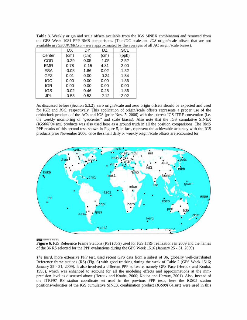
Table 3. Weekly origin and scale offsets available from the IGS SINEX combination and removed fromthe GPS Week 1081 PPP RMS comparisons. (The IGC scale and IGS origin/scale offsets that are notavailable in IGS00P1081.sum were approximated by the averages of all AC origin/scale biases).

DX DY DZ SCLCenter (cm) (cm) (cm) (ppb)COD -0.29 0.05 -1.05 2.52EMR 0.78 -0.15 4.81 2.00ESA -0.08 1.86 0.02 1.32GFZ 0.01 0.00 -0.24 1.34IGC 0.00 0.00 0.00 1.86IGR 0.00 0.00 0.00 0.00IGS -0.02 0.46 0.28 1.86JPL -0.53 0.53 -2.12 2.02

As discussed before (Section 5.3.2), zero origin/scale and zero origin offsets should be expected and usedfor IGR and IGC, respectively. This application of origin/scale offsets represents a proper use of theorbit/clock products of the ACs and IGS (prior Nov. 5, 2006) with the current IGS ITRF convention (i.e.the weekly monitoring of “geocenter” and scale biases). Also note that the IGS cumulative SINEX(IGS00P04.snx) products was also used here as a ground truth in all the position comparisons. The RMSPPP results of this second test, shown in Figure 5, in fact, represent the achievable accuracy with the IGSproducts prior November 2006, once the small daily or weekly origin/scale offsets are accounted for.

algo

yell

drao

kokb

thti

conz lpgs

ohi2 mcm4

cro1

nyal

chpi

asc1

mas1

vill

brusonsa

wtzr

kit3ramo

harb

mbar

nril

pets

tskb

ulab

kunm

guam

kerg

coco

pert

chat

iisc

tidb

aspa

mdvj

Figure 6. IGS Reference Frame Stations (RS) (dots) used for IGS ITRF realizations in 2009 and the namesof the 36 RS selected for the PPP evaluations during the GPS Week 1516 (January 25 - 31, 2009)

The third, more extensive PPP test, used recent GPS data from a subset of 36, globally well-distributedReference frame stations (RS) (Fig. 6) with good tracking during the week of Table 2 (GPS Week 1516;January 25 - 31, 2009). It also involved a different PPP software, namely GPS Pace (Heroux and Kouba,1995), which was enhanced to account for all the modeling effects and approximations at the mm-precision level as discussed above (Heroux and Kouba, 2000; Kouba and Heroux, 2001). Also, instead ofthe ITRF97 RS station coordinate set used in the previous PPP tests, here the IGS05 stationpositions/velocities of the IGS cumulative SINEX combination product (IGS09P04.snx) were used in this

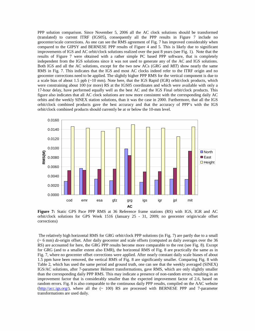
PPP solution comparison. Since November 5, 2006 all the AC clock solutions should be transformed(translated) to current ITRF (IGS05), consequently all the PPP results in Figure 7 include nogeocenter/scale corrections. As one can see the RMS agreement of Fig. 7 has improved considerably whencompared to the GIPSY and BERNESE PPP results of Figure 4 and 5. This is likely due to significantimprovements of IGS and AC orbit/clock solutions realized over the past 8 years (see Fig. 1). Note that theresults of Figure 7 were obtained with a rather simple PC based PPP software, that is completelyindependent from the IGS solutions since it was not used to generate any of the AC and IGS solutions.Both IGS and all the AC solutions, except for the two new ACs (GRG and MIT) show nearly the sameRMS in Fig. 7. This indicates that the IGS and most AC clocks indeed refer to the ITRF origin and nogeocenter corrections need to be applied. The slightly higher PPP RMS for the vertical component is due toa scale bias of about 1.5 ppb (~10 mm). Note here, that the IGS Rapid (IGR) orbit/clock products, whichwere constraining about 100 (or more) RS at the IGS05 coordinates and which were available with only a17-hour delay, have performed equally well as the best AC and the IGS Final orbit/clock products. Thisfigure also indicates that all AC clock solutions are now more consistent with the corresponding daily ACorbits and the weekly SINEX station solutions, than it was the case in 2000. Furthermore, that all the IGSorbit/clock combined products gave the best accuracy and that the accuracy of PPP’s with the IGSorbit/clock combined products should currently be at or below the 10-mm level.

0.0000

0.0020

0.0040

0.0060

0.0080

0.0100

0.0120

0.0140

0.0160

cod emr esa gfz grg igs igr jpl mit

AC

RM

S(M

) NorthEastHeight

Figure 7: Static GPS Pace PPP RMS at 36 Reference frame stations (RS) with IGS, IGR and ACorbit/clock solutions for GPS Week 1516 (January 25 - 31, 2009; no geocenter origin/scale offsetcorrections)

The relatively high horizontal RMS for GRG orbit/clock PPP solutions (in Fig. 7) are partly due to a small(~ 6 mm) dz-origin offset. After daily geocenter and scale offsets (computed as daily averages over the 36RS) are accounted for here, the GRG PPP results become more comparable to the rest (see Fig. 8). Exceptfor GRG (and to a smaller extent also EMR), the horizontal RMS of Fig. 8 are practically the same as inFig. 7, where no geocenter offset corrections were applied. After nearly constant daily scale biases of about1.5 ppm have been removed, the vertical RMS of Fig. 8 are significantly smaller. Comparing Fig. 8 withTable 2, which has used the same period and ground truth, one can see that the weekly averaged (SINEX)IGS/AC solutions, after 7-parameter Helmert transformations, gave RMS, which are only slightly smallerthan the corresponding daily PPP RMS. This may indicate a presence of non-random errors, resulting in animprovement factor that is considerably smaller than the expected improvement factor of 2.6, based onrandom errors. Fig. 8 is also comparable to the continuous daily PPP results, compiled on the AAC website(http://acc.igs.org/), where all the (~ 100) RS are processed with BERNESE PPP and 7-parametertransformations are used daily.

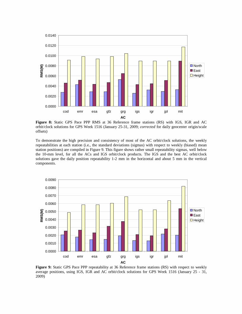
0.0000

0.0020

0.0040

0.0060

0.0080

0.0100

0.0120

0.0140

cod emr esa gfz grg igs igr jpl mit

AC

RM

S(M

) NorthEastHeight

Figure 8: Static GPS Pace PPP RMS at 36 Reference frame stations (RS) with IGS, IGR and ACorbit/clock solutions for GPS Week 1516 (January 25-31, 2009; corrected for daily geocenter origin/scaleoffsets)

To demonstrate the high precision and consistency of most of the AC orbit/clock solutions, the weeklyrepeatabilities at each station (i.e., the standard deviations (sigmas) with respect to weekly (biased) meanstation positions) are compiled in Figure 9. This figure shows rather small repeatability sigmas, well belowthe 10-mm level, for all the ACs and IGS orbit/clock products. The IGS and the best AC orbit/clocksolutions gave the daily position repeatability 1-2 mm in the horizontal and about 5 mm in the verticalcomponents.

0.0000

0.0010

0.0020

0.0030

0.0040

0.0050

0.0060

0.0070

0.0080

0.0090

cod emr esa gfz grg igs igr jpl mit

AC

RM

S(M

) NorthEastHeight

Figure 9: Static GPS Pace PPP repeatability at 36 Reference frame stations (RS) with respect to weeklyaverage positions, using IGS, IGR and AC orbit/clock solutions for GPS Week 1516 (January 25 - 31,2009)

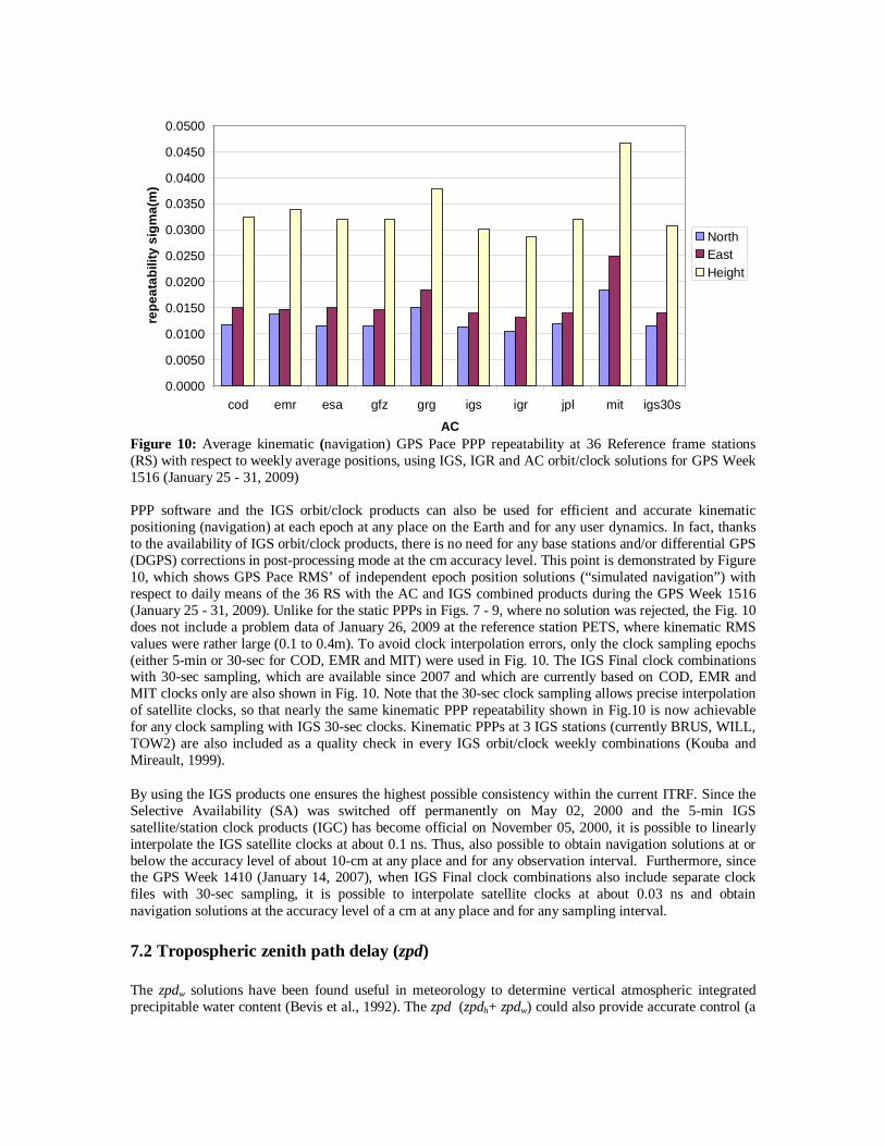
0.0000

0.0050

0.0100

0.0150

0.0200

0.0250

0.0300

0.0350

0.0400

0.0450

0.0500

cod emr esa gfz grg igs igr jpl mit igs30s

AC

rep

eata

bili

ty s

igm

a(m

)

NorthEastHeight

Figure 10: Average kinematic (navigation) GPS Pace PPP repeatability at 36 Reference frame stations(RS) with respect to weekly average positions, using IGS, IGR and AC orbit/clock solutions for GPS Week1516 (January 25 - 31, 2009)

PPP software and the IGS orbit/clock products can also be used for efficient and accurate kinematicpositioning (navigation) at each epoch at any place on the Earth and for any user dynamics. In fact, thanksto the availability of IGS orbit/clock products, there is no need for any base stations and/or differential GPS(DGPS) corrections in post-processing mode at the cm accuracy level. This point is demonstrated by Figure10, which shows GPS Pace RMS’ of independent epoch position solutions (“simulated navigation”) withrespect to daily means of the 36 RS with the AC and IGS combined products during the GPS Week 1516(January 25 - 31, 2009). Unlike for the static PPPs in Figs. 7 - 9, where no solution was rejected, the Fig. 10does not include a problem data of January 26, 2009 at the reference station PETS, where kinematic RMSvalues were rather large (0.1 to 0.4m). To avoid clock interpolation errors, only the clock sampling epochs(either 5-min or 30-sec for COD, EMR and MIT) were used in Fig. 10. The IGS Final clock combinationswith 30-sec sampling, which are available since 2007 and which are currently based on COD, EMR andMIT clocks only are also shown in Fig. 10. Note that the 30-sec clock sampling allows precise interpolationof satellite clocks, so that nearly the same kinematic PPP repeatability shown in Fig.10 is now achievablefor any clock sampling with IGS 30-sec clocks. Kinematic PPPs at 3 IGS stations (currently BRUS, WILL,TOW2) are also included as a quality check in every IGS orbit/clock weekly combinations (Kouba andMireault, 1999).

By using the IGS products one ensures the highest possible consistency within the current ITRF. Since theSelective Availability (SA) was switched off permanently on May 02, 2000 and the 5-min IGSsatellite/station clock products (IGC) has become official on November 05, 2000, it is possible to linearlyinterpolate the IGS satellite clocks at about 0.1 ns. Thus, also possible to obtain navigation solutions at orbelow the accuracy level of about 10-cm at any place and for any observation interval. Furthermore, sincethe GPS Week 1410 (January 14, 2007), when IGS Final clock combinations also include separate clockfiles with 30-sec sampling, it is possible to interpolate satellite clocks at about 0.03 ns and obtainnavigation solutions at the accuracy level of a cm at any place and for any sampling interval.

7.2 Tropospheric zenith path delay (zpd)

The zpdw solutions have been found useful in meteorology to determine vertical atmospheric integratedprecipitable water content (Bevis et al., 1992). The zpd (zpdh+ zpdw) could also provide accurate control (a

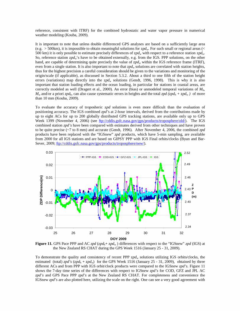
reference, consistent with ITRF) for the combined hydrostatic and water vapor pressure in numericalweather modeling (Kouba, 2009).

It is important to note that unless double differenced GPS analyses are based on a sufficiently large area(e.g. > 500km), it is impossible to obtain meaningful solutions for zpdw. For such small or regional areas (<500 km) it is only possible to estimate precisely differences of zpdw with respect to a reference station zpdw.So, reference station zpdw‘s have to be obtained externally, e.g. from the IGS. PPP solutions, on the otherhand, are capable of determining quite precisely the value of zpdw within the IGS reference frame (ITRF),even from a single station. It is also important to note that zpdw solutions are correlated with station heights,thus for the highest precision a careful consideration should be given to the variations and monitoring of theorigin/scale (if applicable), as discussed in Section 5.3.2. About a third to one fifth of the station heighterrors (variations) map directly into the zpdw solutions (Gendt, 1996, 1998). This is why it is alsoimportant that station loading effects and the ocean loading, in particular for stations in coastal areas, arecorrectly modeled as well (Dragert et al., 2000). An error (bias) or unmodeled temporal variations of Mh,Mw and/or a priori zpdh, can also cause systematic errors in heights and the total zpd (zpdh + zpdw ) of morethan 10 mm (Kouba, 2009).

To evaluate the accuracy of troposheric zpd solutions is even more difficult than the evaluation ofpositioning accuracy. The IGS combined zpd’s at 2-hour intervals, derived from the contributions made byup to eight ACs for up to 200 globally distributed GPS tracking stations, are available only up to GPSWeek 1399 (November 4, 2006) (see ftp://cddis.gsfc.nasa.gov/gps/products/troposphere/old/). The IGScombined station zpd’s have been compared with estimates derived from other techniques and have provento be quite precise (~7 to 8 mm) and accurate (Gendt, 1996). After November 4, 2006, the combined zpdproducts have been replaced with the “IGSnew” zpd products, which have 5-min sampling, are availablefrom 2000 for all IGS stations and are based on GIPSY PPP with IGS Final orbits/clocks (Byun and Bar-Sever, 2009; ftp://cddis.gsfc.nasa.gov/gps/products/troposphere/new/).

-0.03

-0.02

-0.01

0

0.01

0.02

0.03

25 26 27 28 29 30 31 32

DOY 2009

ZD

P D

iffe

ren

ce(m

)

PPP-IGS COD-IGS GFZ-IGS JPL-IGS IGS

2.34

2.37

2.40

2.43

2.46

2.49

2.52

Z P D(m)

Figure 11. GPS Pace PPP and AC zpd (zpdh+ zpdw ) differences with respect to the “IGSnew” zpd (IGS) atthe New Zealand RS CHAT during the GPS Week 1516 (January 25 - 31, 2009).

To demonstrate the quality and consistency of recent PPP zpdw solutions utilizing IGS orbits/clocks, theestimated (total) zpd’s (zpdh + zpdw) for the GPS Week 1516 (January 25 - 31, 2009), obtained by threedifferent ACs and from PPP with IGS orbit/clock products were compared to the IGSnew zpd’s. Figure 11shows the 7-day time series of the differences with respect to IGSnew zpd’s for COD, GFZ and JPL ACzpd’s and GPS Pace PPP zpd’s at the New Zealand RS CHAT. For completeness and convenience theIGSnew zpd’s are also plotted here, utilizing the scale on the right. One can see a very good agreement with

IGSnew zpd for both PPP and JPL AC zpd’s, with a standard deviation of about 2 mm in both cases, thoughboth PPP and JPL AC show a small systematic (negative) offset. This is likely due to the IGSnew zpd,since it uses an old MF (Neill) and only a constant, height dependent pressure for zpdh (Byun and Bar-Sever, 2009), while JPL is using the mandatory global seasonal MF (GMF) model with zpdh based on aglobal pressure model (GPT) (see Boehm at al., 2006 and Boehm at al., 2007, respectively) and the GPSPace PPP is using temporally and specially varying NWM values for Mh, Mw and zpdh (Kouba, 2007).

COD and GFZ AC zpd’s in Fig. 11 also exhibit a similar negative bias, however the agreement is muchworse, with standard deviations of 6 and 7 mm, respectively. This is mainly due to smoothing, caused byCOD hourly or GFZ half-hourly estimations, which could not depict the rapid changes of CHAT zpd onthis day. Furthermore, continuity constraints at the hourly and half-hourly zpd estimation boundaries likelycause the large, compensating spikes for both COD and GFZ zpd’s (see Fig. 11).

To get a more global view of the quality of the PPP zpd estimates, the zpd’s of the above 36 RS static PPPtest have been compared with the IGSnew zpd products. IGSnew zpd products are missing for three RS(NYAL, MDVJ and ASPA) during this GPS Week 1516. Furthermore, on each day and at every station thelast two 5-min epochs (23:50 and 23:55) are also missing in IGSnew zpd’s and thus could not be includedin the comparisons. The 7-day mean zpd differences (PPP-IGSnew) varied from -3 to 4 mm and thestandard deviations varied from 1 to 3 mm, with an average standard deviation of 1.9 mm. However, theIGSnew zpd’s had to be first corrected for height errors by dH/4, where dH is the error (with respect to theIGS05) of the IGSnew daily (i.e., GIPSY PPP) height solutions, which are also available in the IGSnew zpdfiles. Otherwise, without the height corrections, the mean zpd biases were between –12 (at MCM4) and 3mm. This is a consequence of the old MF and a constant, height dependent station pressures (used for zpdh)utilized for the IGSnew. Recall that the GPS Pace PPP has used temporal1ly and spatially varying zpdh andthe MF’s of the gridded VMF1 (Kouba 2007). The zpdw solution precision of 3 mm corresponds to about0.5 mm of integrated precipitable water (Bevis et al., 1992).

7.3 Station clock solutions

It is important to note that it is impossible to get meaningful clock solutions from double difference GPSanalyses, which is the penalty paid for the significant simplification and efficiency of double differencedGPS observations. The clock solutions are only possible in un-differenced global and PPP solutions. Theclock solution parameters are perhaps the most sensitive to a wide range of effects and thus can besignificantly biased unless properly modeling all the effects discussed above (Section 5), including theocean loading effects. For these reasons, discussions in Section 5.2.3 should also be carefully consulted.

Evaluating the quality of PPP station clock solutions is also somewhat complicated by the absence of anabsolute standard for comparison and the fact that different reference clocks and alignment values are usedby the ACs in the computation of their daily solutions. Therefore, the following evaluation is an internalcomparison of the above (static) GPS Pace PPP station clock solutions, based on the combined IGS Final(igs) and Rapid (igr) satellite orbits/clocks at only one of the 36 RS, during the GPS Week 1516. The IGSRS BRUS was selected for this clock comparison since it is equipped with a Hydrogen MASER (HM)clock and was processed by most ACs during this week.

Figure 12 shows the igr and igs BRUS station PPP clock solutions and their differences with respect to theIGS Final and Rapid combined clocks (IGS, IGR) during the 7 days of the GPS Wk 1516. Except for smalloffsets and drifts, both the igr and igs PPP clocks agree very well with the IGS and IGR ones, namely atthe 12 and 14 picosecond levels (one standard deviation). The small daily jumps and drifts should beexpected and are mainly due to the PPP clocks, since PPP (as well as AC) clocks are aligned daily bypseudorange averages for PPP observed at a single station, and for ambiguity fixed AC solutions also at theneighbouring stations. Consequently AC station clocks should have smaller jumps and drifts than thecorresponding PPP ones. Furthermore, the current IGS clock combination and time scale alignment (Senioret al. 2001) was designed to minimize the daily AC clock jumps, which otherwise could exceed 1 ns atsome stations for some AC solutions (Ray and Senior 2002). To minimize the HM aging and other non-liner effects (such as residual reference clock errors (instabilities) of the IGS/AC clocks, the igs and igr

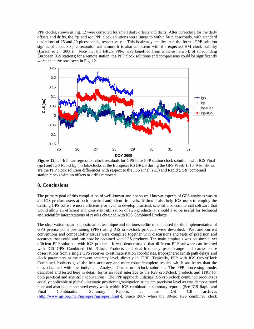
PPP clocks, shown in Fig. 12 were corrected for small daily offsets and drifts. After correcting for the dailyoffsets and drifts, the igs and igr PPP clock solutions were linear to within 50 picoseconds, with standarddeviations of 25 and 29 picoseconds, respectively. This is already smaller than the formal PPP solutionsigmas of about 30 picoseconds, furthermore it is also consistent with the expected HM clock stability(Larson et al., 2000). Note that the BRUS PPPs have benefited from a dense network of surroundingEuropean IGS stations; for a remote station, the PPP clock solutions and comparisons could be significantlyworse than the ones seen in Fig. 12.

-0.15

-0.1

-0.05

0

0.05

0.1

0.15

0.2

0.25

25 26 27 28 29 30 31 32

DOY 2009

CL

K(n

s)

igsigrigr-IGRigs-IGS

Figure 12. 24-h linear regression clock residuals for GPS Pace PPP station clock solutions with IGS Final(igs) and IGS Rapid (igr) orbits/clocks at the European RS BRUS during the GPS Week 1516. Also shownare the PPP clock solution differences with respect to the IGS Final (IGS) and Rapid (IGR) combinedstation clocks with no offsets or drifts removed.

8. Conclusions

The primary goal of this compilation of well-known and not so well known aspects of GPS analyses was toaid IGS product users at both practical and scientific levels. It should also help IGS users to employ theexisting GPS software more efficiently or even to develop practical, scientific or commercial software thatwould allow an efficient and consistent utilization of IGS products. It should also be useful for technicaland scientific interpretations of results obtained with IGS Combined Products.

The observation equations, estimation technique and station/satellite models used for the implementation ofGPS precise point positioning (PPP) using IGS orbit/clock products were described. Past and currentconventions and compatibility issues were compiled together with discussions and tests of precision andaccuracy that could and can now be obtained with IGS products. The main emphasis was on simple, yetefficient PPP solutions with IGS products. It was demonstrated that different PPP software can be usedwith IGS GPS Combined Orbit/Clock Products and dual-frequency pseudorange and carrier-phaseobservations from a single GPS receiver to estimate station coordinates, tropospheric zenith path delays andclock parameters at the mm-cm accuracy level, directly in ITRF. Typically, PPP with IGS Orbit/ClockCombined Products gave the best accuracy and more robust/complete results, which are better than theones obtained with the individual Analysis Center orbit/clock solutions. The PPP processing mode,described and tested here in detail, forms an ideal interface to the IGS orbit/clock products and ITRF forboth practical and scientific applications. The PPP approach utilizing IGS orbit/clock combined products isequally applicable to global kinematic positioning/navigation at the cm precision level as was demonstratedhere and also is demonstrated every week within IGS combination summary reports. (See IGS Rapid andFinal Combination Summary Reports at the IGS CB archives(http://www.igs.org/mail/igsreport/igsreport.html)). Since 2007 when the 30-sec IGS combined clock

products have become available and with no SA, it is possible to precisely interpolate satellite clocks,which enables also cm global kinematic positioning (navigation) at any interval sampling, anywhere in theworld and without any need of base stations.

Acknowledgements

IGS data and products are the result of an unprecedented voluntary, yet coordinated effort of manyindividuals and organizations that continues to provide an invaluable service to scientific and technicalcommunity. A part of the above information, mainly pertaining to the PPP modeling and some of the resultevaluations, have already been presented and published in a summary form at the 2000 IGS NetworkWorkshop (Héroux and Kouba, 2000) and in Kouba and Héroux (2001). The former and the currentAnalysis Center Coordinators, R. Weber of Technical University of Vienna and Jim Ray of NGS, as well asJake Griffiths of NGS have read this paper and provided the author with a number of corrections and usefulsuggestions.

References

Agnew, D.C., 1996, SPOTL: Some programs for ocean-tide loading, SIO Ref. Ser. 96-8, Scripps Inst. ofOceanography, La Jolla, California.

Bar-Sever, Y. E., 1996, A new module for GPS yaw attitude control, Proceedings of IGS Workshop-Special Topics and New Directions, eds. G.Gendt and G. Dick, GeoforschunsZentrum, Potsdam, pp. 128-140.

Bar-Sever, Y.E., 1998, Estimation of GPS Transmit Antenna Phase Center offsets, presented at the AGUFall Meeting, EOS Transaction, 79 (45), 183, Nov. 10.

Beutler, G., J. Kouba, and T. Springer, 1995, Combining the Orbits of the IGS Analysis Centers, Bull.Geod. 69, pp. 200-222.

Bevis M, Businger S, Herring T, Rocken C, Anthes R, Ware RH, 1992, GPS meteorology: remote sensingof atmospheric water vapor using the global positioning system. J Geophys Res 97(D14):15787–15801

Boehm J, Schuh H (2004) Vienna Mapping Functions in VLBI analyses, Geophys. Res. Lett. 31, L01603,doi:10.1029/2003GL018984

Boehm J, Niell A, Tregoning, P, Schuh H (2006) Global Mapping Function (GMF): A new empiricalmapping function based on numerical weather model data, Geophys. Res. Lett. 33, L07304,doi:10.1029/2005GL025546

Boehm J, Heinkelmann R, and Schuh H (2007) Short Note: A global model of pressure and temperature forgeodetic applications, Journal of Geodesy , doi:10.1007/s00190-007-0135-3

Byun S. H. and Y. E. Bar-Sever, 2009, A new type of troposphere zenith path delay product of theInternational GNSS Service, J Geod (2009) 83:367–373 DOI 10.1007/s00190-008-0288-8

Dach, R. Hugentobler, U. Fridez, P. and Meindl, M., 2007, Bernese GPS Software Version 5.0,Astronomical Institute, University of Berne, pp. 612.

Dow J.M., Neilan R.E., Gendt G. , 2005, The International GPS Service (IGS): Celebrating the 10th

Anniversary and Looking to the Next Decade, Adv. Space Res. 36 vol. 36, no. 3, pp. 320-326, 2005.doi:10.1016/j.asr.2005.05.125

Dow J., J. Perez, T. Springer, C. Garcia, I. Romero, J. Feltens , E. Rojo, J. Fernandez ,Y. Andres, R.Zandbergen, A. Ballereau , 2006, IGS Activities at ESA / ESOC. IGS Workshop 2006, Darmstadt,Germany. May 8-11, 2006.ftp://igs.org/pub/resource/pubs/06_darmstadt/IGS%20Posters%20PDF/p_18_Springer.pdf

Dragert, H., T.S. James, and A. Lambert, 2000, Ocean Loading Corrections for Continuous GPS: A CaseStudy at the Canadian Coastal Site Holberg, Geophysical Research Letters, Vol. 27, No. 14, pp. 2045-2048, July 15, 2000.

Collins, P., 2008, Isolating and estimating undifferenced GPS Integer ambiguities. A paper presented at theION 2008 Technical Meeting, San Diego, Cal., January 28-30.

Ferland, R., 2000, ITRF Coordinator Report, 1999 IGS Annual Report, IGS Central Bureau, Jet PropulsionLaboratory, Pasadena, CA, pp.28-31, ftp://igs.org/igscb/resource/pubs/1999_IGS_AnnRep.pdf,

Ferland, R., 2001, ITRF Coordinator Report, 2000 IGS Annual Report, IGS Central Bureau , Jet PropulsionLaboratory, Pasadena, CA, pp.24-28, ftp://igs.org/igscb/resource/pubs/2000_an_rpt.pdf.

Ferland, R., Z. Altamimi, C. Bruynx, M. Craymer, H. Habrich and J. Kouba, 2002, Regional networkdensifications, Proceedings of IGS Network, Data and Analysis Center Workshop 2002, held in Ottawa,Canada, April 8-11 (http://www.igs.org/overview/pubs/ottawa_ws.html ).

Gendt, G., G. Dick, W. Soehne ,1999, GFZ Analysis Center of IGS- Annual Report, 1998 IGS TechnicalReports, IGS Central Bureau, Jet Propulsion Laboratory, Pasadena, CA, (eds K. Gowey, R. Neilan, A.Moore), November, pp. 79-87.

Gendt, G., 1998, IGS Combination of Tropospheric Estimates – Experience from Pilot Experiment,Proceedings of 1998 IGS Analysis Center Workshop, J.M. Dow, J. Kouba and T. Springer, Eds. IGSCentral Bureau, Jet Propulsion Laboratory, Pasadena, CA, pp. 205-216.

Gendt, G., 1996, Comparison of IGS Troposphere Estimations, Proceedings of 1996 IGS Analysis CenterWorkshop, R.E. Neilan, P.A. Van Scoy and J.F. Zumberge, Eds. IGS Central Bureau, Jet PropulsionLaboratory, Pasadena, CA, pp. 151-164.

Ghoddousi-Fard R. and P. Dare, 2005, Online GPS processing services: an initial study, GPS Solutions,Vol. 10, No. 1, pp. 12-20, doi: 10.1007/s10291-005-0147-5

Hamilton, W.C., 1964, Statistics in Physical Science, Ronald, New York.

Héroux, P. and J. Kouba, 1995, GPS Precise Point Positioning with a Difference, Paper presented atGeomatics ’95, Ottawa, Ontario, Canada, June 13-15.

Héroux, P., M. Caissy, and J. Gallace, 1993, Canadian Active Control System Data Acquisition andValidation, Proceedings of the 1993 IGS Workshop, University of Bern, pp. 49-58.

Héroux, P. and J. Kouba, 2001, GPS Precise Point Positioning Using IGS Orbit Products, Phys. Chem.Earth (A), Vol. 26, No.6-8, pp. 573-578.

Hofmann-Wellenhof, B., Lichtenegger, H., Collins, J., 1997, GPS - Theory and Practice, 4th revisededition, Springer, Wien - New York.

ICD-GPS-200, 1991, Interface control document, NAVSTAR GPS Space Segment, July 3.

IERS, 1989, IERS Standards (1989), IERS Technical Note 3, D.D. McCarthy (ed.)

IERS, 1996, IERS Conventions (1996), IERS Technical Note 21, D.D. McCarthy (ed.), (see alsohttp://maia.usno.navy.mil/conventions.html; ftp://maia.usno.navy.mil/conventions/)

IERS, 2003, IERS Conventions (2003), IERS Technical Note 32, DD. McCarthy and G. Petit (eds.), (seealso http://tai.bipm.org/iers/conv2003/conv2003.html and the updates: ftp://tai.bipm.org/iers/convupdt/)

ION, 1980, Global Positioning System, Vol. I, Papers published in NAVIGATION,ISBN: 0-936406-00-3.

King, R. W., and Y. Bock, 1999, Documentation of the GAMIT GPS Analysis Software (version 9.8),Unpublished, Massachusetts Institute of Technology, Cambridge, Massachusetts.

Kouba, J., 1998, IGS Analysis Activities, 1998, IGS Annual Report, IGS Central Bureau, Jet PropulsionLaboratory, Pasadena, CA, pp. 13-17.

Kouba, J., J.R. Ray and M.M. Watkins, 1998, IGS Reference Frame realization, Proceedings of 1998 ACWorkshop held in Darmstadt, Germany, 9-11 Feb., (ed. by J.M. Dow et al.), pp. 139-172.

Kouba, J. and J. Popelar, 1994, Modern Reference Frame for Precise Satellite Positioning and Navigation,1994, Proceedings of the Inter. Symp. on Kinematic Systems in Geodesy, Geomatics & Navigation (KIS94), Banff, Canada, Aug., 1994, pp. 79-86.

Kouba, J., Y. Mireault, G. Beutler, T. Springer, 1998, A Discussion of IGS Solutions and Their Impact onGeodetic and Geophysical Applications, GPS Solutions, Vol. 2, No. 2, pp. 3-15.

Kouba, J. and Y. Mireault, 1999, 1998 Analysis coordinator Report, 1998 Technical Reports, IGS CentralBureau, Jet Propulsion Laboratory, Pasadena, CA, (eds. K. Gowey, R.E. Neilan and A. Moore), November,pp.15-58.

Kouba, J. and P. Héroux, 2001, Precise Point Positioning Using IGS Orbit and Clock Products, GPSSolutions, Vol. 5, No.2, pp.12-28.

Kouba, J. and T. Springer. 2001, New IGS Station and Clock Combination, GPS Solutions, Vol. 4, No. 4,pp. 31-36.

Kouba, J., 2002a, The GPS Toolbox ITRF Transformations, GPS Solutions, Vol. 5, No. 3, pp.88-90.

Kouba, J., 2002b, Sub-daily Earth Rotation Parameters and the International GPS Service Orbit/ClockSolution Products, Studia Geophysica et Geodetica 46 (2002), pp.9-25.

Kouba, J., 2002c, Relativistic Time Transformations in GPS, GPS Solutions, Vol. 5, No 4 , pp.1-9.

Kouba, J., 2004, Improved relativistic transformations in GPS, GPS Solutions 2004, doi:10.1007/s10291-004-102-x.

Kouba J (2007) Implementation and testing of the gridded Vienna Mapping Function 1 (VMF1), Journal ofGeodesy , doi:10.1007/s00190-007-0170-3

Kouba, J., 2008, A simplified yaw-attitude model for eclipsing GPS satellites, GPS Solutions 2008: DOI:10.1007/s10291-008-0092-1

Kouba, J., 2009, Testing of global pressure/temperature (GPT) model and global mapping function (GMF)in GPS analyses. J Geod (2009) 83 (3), , pp. 199-208, DOI: 10.1007/s00190-008-0229-6

Larson, K.M., J. Levine, L.M. Nelson, 2000, Assessment of GPS Carrier-Phase Stability for Time-TransferApplications. IEEE Transactions on Ultrasonics, Ferroelectrics and Frequency Control, Vol. 47, No. 2,March 2000.

Lichten, S.M., Y.E. Bar-Sever, E.I. Bertiger, M. Heflin, K. Hurst, R.J. Muellerschoen, S.C. Wu, T.P.Yunck, and J. F. Zumberge, 1995, GIPSY-OASIS II: A High precision GPS Data processing System andgeneral orbit analysis tool, Technology 2006, NASA Technology Transfer Conference, Chicago, Il., Oct.24-26.

Neilan, R.E., Zumberge, J.F., Beutler, G., and J. Kouba, 1997, The International GPS Service: A globalresource for GPS applications and research. In Proc. ION-GPS-97 (pp. 883-889). The Institute ofNavigation.

Pagiatakis,S.D., 1992, Program LOADSDP for the calculation of ocean load effects, Man. Geod., 17, 315-320.

Ray, J. and K. Senior, 2002, IGS/BIPM Pilot Project: GPS Carrier Phase for Time/ Frequency Transfer andTime Scale Formation, Proceedings of IGS Network, Data and Analysis Center Workshop 2002, held inOttawa, Canada, April 8-11 (in prep).

Ray, J. and J. Griffiths — Overview of IGS products & Analysis Center modeling, a paper presented at IGSAnalysis Center Workshop 20082-6 June 2008 (http://www.ngs.noaa.gov/IGSWorkshop2008/prog.html),Miami Beach, Florida, USA

Rothacher, M., S. Schaer, L. Mervart and G. Beutler, 1995, Determination of Antenna Phase centerVariations Using GPS Data, Proceedings of 1995 IGS Workshop on Special Topics and New Directions,eds G. Gent an G. Dick, pp. 77-92, GeoForshungsZentrum, Potsdam, Germant, May 15-18.

Rothacher, M and G. Mader, 2002, Receiver and Satellite Antenna Phase Center Offsets and Variations,Proceedings of IGS Network, Data and Analysis Center Workshop 2002, held in Ottawa, Canada, April 8-11 (http://www.igs.org/overview/pubs/ottawa_ws.html ).

Schenewerk, M., W. Dillinger, G. Mader, 1999, NOAA/NGS Analysis Strategy Summary, 1998 IGSTechnical Reports, IGS Central Bureau, at JPL, (eds K. Gowey, R. Neilan, A. Moore), November, pp. 99-105.

Scherneck, H.G. , 1991, A parameterized Solid Earth Tide Model and Ocean Tide Loading Effects forglobal geodetic baseline measurements, Geophs. J. Int. 106, pp. 677-694.

Scherneck, H.G. , 1993, Ocean Tide Loading: Propagation errors from ocean tide into loading coefficients,Man. Geodetica, 18, pp.59-71.

Schmid, R., R. Steigenberger, G. Gendt, M. Ge and M. Rothacher, 2007, Generation of a consistentabsolute phase center correction model for GPS receiver and satellite antennas. Jour. of Geodesy, Volume81, No. 12, pp. 781-798, doi: 10.1007/s00190-007-0148-y.

Senior, K. Koppang P., Matsakis D., Ray J., 2001, Developing an IGS time scale, Proceedings IEEE Freq.Contr. Symposium, June 6-8, 2001, pp. 211-218.

Springer, T. A., 1999, Positioning, Timing and Ranging Using the Global Positioning System, PhD Thesis,Universitat Bern.

Springer, T., J. Kouba, and Y. Mireault., 2000, 1999 Analysis Coordinator Report, in 1999 IGS TechnicalReports, IGS Central Bureau, Jet Propulsion Laboratory, Pasadena, CA(ftp://igs.org/igscb/resource/pubs/99_tec/99tr_analysis_center_2.pdf).

Vaníček P. and E..J. Krakiwsky, 1986, Geodesy: The Concept, 2nd edn., North-Holland, 617 pp.

Wahr, J.M., 1981, The forced nutation of an elliptical, rotating, elastic, and ocean less Earth, Geophys. J.Roy. Astron. Soc., 64, pp. 705-727.

Weber, R., C. Bruyninx, H.G. Scherneck, M.Rothacher, P.H.Anderson, T.F.Baker, T.van Dam, 2002, TidalEffects in GPS/GLONASS Data Processing, in Proceedings of Journees 2001, (in print).

Weber, R., J. Ray and J. Kouba, 2002, Review of IGS Analysis Products, Proceedings of IGS Network,Data and Analysis Center Workshop 2002, held in Ottawa, Canada, April 8-11(http://www.igs.org/overview/pubs/ottawa_ws.html ).

Wu, J.T., S,C. Wu, G.A. Hajj, W.I. Bertiger, and S.M. Lichten, 1993, Effects of antenna orientation onGPS carrier phase, Man. Geodetica 18, pp. 91-98.Zumberge, J. and Gent G., 2000, The Demise of selectiveavailability and implication for the International GPS Service, position paper presented at the IGS NetworkWorkshop 2000, held in Oslo, Norway, July, Phys. Chem. Earth (A), Vol. 26, No.6-8.

Zumberge, J.F., Heflin, M.B., Jefferson, D.C., Watkins, M.M., and F.H. Webb, 1997, Precise pointpositioning for the efficient and robust analysis of GPS data from large networks. J. Geophys. Res., 102,5005-5017.