Embed Size (px)
Citation preview

A Geospatial Web Application (GEOWAPP) for Supporting Course Laboratory
Practices in Surveying Engineering
by
Jaime Garbanzo
Surveying Ingineer, Universidad de Costa Rica
A Thesis Submitted in Partial Fulfillment
of the Requirements for the Degree of
Master of Science Engineering
in the Graduate Academic Unit of Geodesy and Geomatics
Supervisors: Emmanuel Stefanakis, PhD, Geodesy & Geomatics Engineering.
Robert William Kingdon, PhD, Geodesy & Geomatics Engineering.
Examining Board: Peter Dare, PhD, Geodesy and Geomatics Engineering.
Vassilis Gikas, PhD, Rural and Surveying Engineering.
This thesis is accepted by the
Dean of Graduate Studies
THE UNIVERSITY OF NEW BRUNSWICK
September, 2015
@ Jaime Garbanzo, 2015
ii
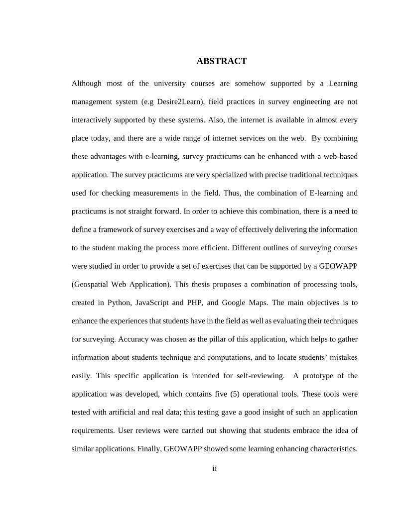
ABSTRACT
Although most of the university courses are somehow supported by a Learning
management system (e.g Desire2Learn), field practices in survey engineering are not
interactively supported by these systems. Also, the internet is available in almost every
place today, and there are a wide range of internet services on the web. By combining
these advantages with e-learning, survey practicums can be enhanced with a web-based
application. The survey practicums are very specialized with precise traditional techniques
used for checking measurements in the field. Thus, the combination of E-learning and
practicums is not straight forward. In order to achieve this combination, there is a need to
define a framework of survey exercises and a way of effectively delivering the information
to the student making the process more efficient. Different outlines of surveying courses
were studied in order to provide a set of exercises that can be supported by a GEOWAPP
(Geospatial Web Application). This thesis proposes a combination of processing tools,
created in Python, JavaScript and PHP, and Google Maps. The main objectives is to
enhance the experiences that students have in the field as well as evaluating their techniques
for surveying. Accuracy was chosen as the pillar of this application, which helps to gather
information about students technique and computations, and to locate students’ mistakes
easily. This specific application is intended for self-reviewing. A prototype of the
application was developed, which contains five (5) operational tools. These tools were
tested with artificial and real data; this testing gave a good insight of such an application
requirements. User reviews were carried out showing that students embrace the idea of
similar applications. Finally, GEOWAPP showed some learning enhancing characteristics.

iii
However, a test with a real course remains to be carried out to determine whether it is
beneficial to students.

iv
ACKNOWLEDGEMENTS
To the University of Costa Rica that provided the funding for this research.
To my Supervisors Dr. Robert Kingdon and Dr. Emmanuel Stefanakis, who provided
guidance and the opportunity to finish this program.

v
Table of Contents
A Geospatial Web Application (GEOWAPP) for Supporting Course Laboratory Practices
in Surveying Engineering ................................................................................................... 1
ABSTRACT ........................................................................................................................ ii
ACKNOWLEDGEMENTS ............................................................................................... iv
Chapter 1. Introduction ....................................................................................................... 1 1.1 Introduction .......................................................................................................... 1
1.2 State of the art ...................................................................................................... 2
1.3 Definitions of the Research Questions / Hypothesis ............................................ 4
1.3.1 Hypothesis..................................................................................................... 4
1.3.2 Research Questions. ...................................................................................... 5
1.3.3 Research objectives (RO) ............................................................................. 6
Chapter 2. Application Design ............................................................................................ 7 1.1 Modeling .............................................................................................................. 7
1.1.1 Global Architecture ....................................................................................... 7
1.2 Exercises’ schemata ........................................................................................... 11
1.2.1 Review of GGE’s field practices exercises ................................................. 11
1.3 How to Test Accuracies ..................................................................................... 17
1.4 Required tools for testing accuracies ................................................................. 18
1.4.1 Traversing comparator ................................................................................ 18
1.4.2 Leveling Tools ............................................................................................ 20
1.4.3 Network comparator ................................................................................... 27

vi
1.4.4 Topographic survey comparator ................................................................. 27
1.5 Database Design ................................................................................................. 41
1.6 Authoring tool .................................................................................................... 42
Chapter 3: GEOWAPP prototype development ............................................................... 43 1.7 Application Structure ......................................................................................... 44
1.7.1 Forms .......................................................................................................... 45
1.7.2 PHPS Folder................................................................................................ 46
1.7.3 CSS, fonts, and JS folders ........................................................................... 48
1.7.4 REPORTS, img, uploads folders, and KMLS ............................................ 48
1.7.5 Python Folder .............................................................................................. 48
1.8 The GEOWAPP interface (Index.php ).............................................................. 49
1.9 Toolbox .............................................................................................................. 52
1.9.1 Traversing Comparator ............................................................................... 53
1.9.2 Leveling Comparator .................................................................................. 60
1.9.3 Least squares leveling ................................................................................. 62
1.9.4 Proximity Comparator ................................................................................ 64
1.9.5 Vertical Comparator.................................................................................... 72
1.10 Database Implementation ............................................................................... 77
Chapter 4: Testing and Evaluation of GEOWAPP ........................................................... 79 1.11 Traversing Comparator. .................................................................................. 79
vii
1.12 Leveling Comparator and Least Squares tool................................................. 82
1.13 Proximity Comparator tool ............................................................................. 83
1.14 Vertical Comparator tool ................................................................................ 85
1.15 User Reviews .................................................................................................. 90
Chapter 5: Discussion on the outcomes. ........................................................................... 94
Chapter 6: Conclusions. .................................................................................................... 98
References ....................................................................................................................... 101
Appendices ...................................................................................................................... 106 1.16 Appendix 1: GEOWAPP installation. .......................................................... 106
1.17 Appendix 2: User Review survey sheet. ....................................................... 112
1.18 User Guide .................................................................................................... 115
1.18.1 Register ..................................................................................................... 115
Sign in ..................................................................................................................... 115
1.18.2 Traversing comparator: ............................................................................. 115
1.18.3 Leveling Comparator: ............................................................................... 117
1.18.4 Least squares leveling tool: ....................................................................... 118
1.18.5 Proximity Comparator: ............................................................................. 119
Vertical Comparator................................................................................................ 120
Curriculum Vitae

viii
List of Tables
Table 2.1 Exercises classes classified by course .............................................................. 16
Table 2.2: Exercises classes classified by course ............................................................. 16
Table 2.3: Proposed format of the Bowditch rule report .................................................. 20
Table 2.4: Order of accuracies of a leveling network. ...................................................... 24
Table 2.5: Specification of the code system for the survey practicums. ........................... 29
Table 2.6: Acceptable internal error for different classes of survey ................................. 30
Table 2.7 Feature tolerance value ..................................................................................... 35
Table 2.8 statistical measures for accuracy when the Gaussian distribution is met. ........ 37
Table 3.1: Technologies and functionality ........................................................................ 44
Table 3.2: Comparison of GEOWAPP and CTS transformed coordinates ...................... 58
Table 3.3: computation of the total tolerance. In other words, computation of the CEP
radius. ................................................................................................................................ 66
Table 4.1: students2015 data form GGE 2012.................................................................. 80

ix
List of Figures
Figure 2.1: The yellow ellipses show the services that will be provided to the students and
the instructors. ..................................................................................................................... 8
Figure 2.2: This UML component diagram describes the GEOWAPP. ............................. 9
Figure 2.3 This activity diagram shows the different actions that will be carried out by
GEOWAPP. ...................................................................................................................... 10
Figure 2.4: This figure shows an example of the schema, which contains useful information
for students ........................................................................................................................ 20
Figure 2.5: This figure shows the main concepts of differential leveling where the
instrument should be always parallel to the local gravity field. B.S. and F.S. stand for
Backsight and Foresight. Source: own elaboration........................................................... 21
Figure 2.6 shows the students report schema for the differential leveling. ...................... 23
Figure 2.7: a sketch of a topographic survey is shown in which the least squares will be
applied. BM1 is a known Benchmark and BCD are new benchmark that will be measured.
........................................................................................................................................... 24
Figure 2.8: this figure shows the schema definition of the students report using the Leveling
Least Squares Checking tool. ............................................................................................ 26
Figure 2.9: this figure shows the schema definition of the student report for station x. ... 27
Figure 2.10: The EDMs error propagates along line of sight from the observer while σi
(radians) propagates across the line of sight; . The SFE is added to both errors (EDMs error
and σi)................................................................................................................................ 32

x
Figure 2.11: This figure shows a comparison between the TF and the surveyed feature by
students. In Figure 11-A, the TF is in tolerance while in Figure 11-B, this feature is off
tolerance ............................................................................................................................ 34
Figure 2.12: This figure shows the proposed report schema after a DEM or TIN has been
evaluated. .......................................................................................................................... 38
Figure 2.13: this figure shows the report schema 2 for second approach. ........................ 40
Figure 2.14: this figure shows the outlier report schema; PTX and PTY are outliers, which
have residuals bigger than 3σ ........................................................................................... 40
Figure 2.15. Component diagram of the Database shows the classification of the tables that
will be stored in the database ............................................................................................ 41
Figure 3.1: application folders. ......................................................................................... 45
Figure 3.2 The Traverse Checking Form is a static form, which will always display the
same information. ............................................................................................................. 46
Figure 3.3: This figure shows a form generated dynamically for the traversing checking. If
the input values vary in the previous form (Figure 3.2), this form will vary as well. ...... 47
Figure 3.4: this figure shows the loading function, which calls the form displayer and loads
the traverse form into the file. ........................................................................................... 49
Figure 3.5 the xml schema shows the structure of the GEOWAPP interface. There are two
classes of functions: for managing the interface contents and for managing the Google
Maps API. Then, there are two main components in the user interface: the tool bar and the
results displayer. ............................................................................................................... 50
Figure 3.6: this figure shows the appearance of the GEOWAPP in large screens. .......... 51
Figure 3.7: this figure shows the appearance of the GEOWAPP in small screens. .......... 52

xi
Figure 3.8: this figure shows the first type of traverse, which stars in a point and finishes
in a different one. The traverse data shown in this figure was generated synthetically with
a Matlab script................................................................................................................... 54
Figure 3.9: this figure shows the first type of traverse, which starts and finishes the same
point. The traverse data shown in this figure was generated synthetically with a Matlab
script. ................................................................................................................................. 54
Figure 3.10: the UML activity diagram shows the Traverse tool processing flow as well as
the interaction of the different technologies involved, JavaScript, PHP, and Python. ..... 56
Figure 3.11: students will access this information when they are using the tool by
themselves. The residuals, linear misclosure and traverse length are in meters. .............. 59
Figure 3.12: this information will be added to the information displayed in figure 3.11 when
an instructor is using Traversing Comparator. The latitudes, departures, distances and
coordinates are in meters. ................................................................................................. 59
Figure 3.13: the UML activity diagram shows the Levelling tool processing flow as well
as the interaction of the different technologies involved, JavaScript, PHP, and Python. . 61
Figure 3.14: the full report, visible just for instructors, is composed of a detailed
computation (m) and the piece of information given to students as feedback.................. 62
Figure 3.15: the UML activity diagram shows the Least Squares tool processing flow as
well as the interaction of the different technologies involved, JavaScript, Php, and Python.
........................................................................................................................................... 63
Figure 3.16: the first table shows the full report composed by the results of the observation
equation (m), weights, and residuals (m). The second table provides the final elevation (m)
of the unknown and the standard deviations (m). ............................................................. 64
xii
Figure 3.17: as EDM error (𝛔𝐄𝐃𝐌) and internal angle error (𝛔𝐢 𝐢𝐧 𝐦𝐞𝐭𝐞𝐫𝐬) are
independent error, they should be added in square form and then square rooted to compute
the magnitude of the error combination. ........................................................................... 65
Figure 3.18: the CSV file has to have the headers. The order of the columns does not matter.
The units of the coordinates are meters ............................................................................ 67
Figure 3.19: the proximity tool is represented with the name of overall accuracy in
GEOWAPP. The information flow is straightforward. A student who fails inputting the
data has to start again. ....................................................................................................... 68
Figure 3.20: the pinpoints represent the known topographic features (KTF). The green
pinpoint represent the in-tolerance features while red pinpoints represent off-tolerance
features. A textbox shows the distance (m) from a KTF to a SOTF. ............................... 70
Figure 3.21: this report shows the distances (m) from KTF to the closest SOTF with the
same codes. At the end, a RMS value shows the quality of the survey. ........................... 71
Figure 3.22: this CSV file have to have an Id, Y and X coordinate, and height (Z). In
addition, the delimiter can be a semicolon (;) or a comma (,). The units of the coordinates
are meters. ......................................................................................................................... 72
Figure 3.23: this report shows the distances from KTF to the closest SOTF with the same
codes. At the end, a RMS value shows the quality of the survey. .................................... 73
Figure 3.24: Python carries the heavy computation while PHP eases the information flow.
On the other hand, JavaScript helps to display the results. ............................................... 73
Figure 3.25: the blue pinpoints represent KGPs while the red or green pinpoints represent
SOGP. SOGP are the center of the circular residuals. In this case, the accuracy polygons
xiii
have a maximum number of five (5), number of points used for interpolating plus one (1)
, and a minimum number of sides equal to three (3). ....................................................... 75
Figure 3.26: the report shows the id of the points involved in the interpolation, the KGP Z
values (Zkn), the interpolated Z value (Zint), and the residuals (res). In addition, this report
includes the RMS value of the interpolation and the residuals’ mean .............................. 76
Figure 3.27: <<PK>> stands for primary key while <<AK>> for alternative key. In every
table, the name of the field is first specified followed by the field type separated for a colon
(:). ...................................................................................................................................... 78
Figure 4.1: the traverse is represented by a KML polyline on Google Maps. .................. 81
Figure 4.2: the red pinpoints show that no point is within the tolerance. Moreover, the
textbox shows how far apart (in m) the KTF with code BL is from a point from the tested
dataset. .............................................................................................................................. 84
Figure 4.3: the accuracy polygons are built using data from 2013 and 2014 survey
practicum as KGP and SOGP respectively. KGP is shown as blue pinpoint while the SOGP
is shown as green and red pinpoints. ................................................................................ 86
Figure 4.4: the data subject has a circular residual assigned. The in-tolerance circular
residual are almost indistinguishable. ............................................................................... 87
Figure 4.5: Accuracy polygons and the SOGP are shown in the surrounding area of a
parking lot in UNB............................................................................................................ 89
Figure 4.6 : Accuracy polygons are shown on the Google Earth street view option ........ 89
Figure 4.7 The user review results are summarized by question. Also, a table shows the
values for every question. The visual stimulation and blunder detection question do not
include the leveling tool. In addition, the blunder detection shown in the chart refers to

xiv
visually detecting them with the aid of the contextual information provided by Google
Maps. ................................................................................................................................. 91
Figure 4.8: students’ feelings about the concept is shown in this chart. The dark column
shows the evaluation of every tool while the lighter one shows the mean value that includes
every tool. ......................................................................................................................... 93

1
Chapter 1. Introduction
1.1 Introduction
The accelerated development of technologies is clearly affecting our behavior
today. For example, social media, like Facebook and Twitter, is affecting the way people
interact and share information with each other. When there is a need for group interaction,
this is filled through a social group or blog on the Internet. Many companies like ESRI and
Matlab are aware of this situation, and they create institutional forums where people can
place their specific questions and receive help. Also, the market is evolving into a web
services based approach; companies are trying to offer services instead of program installed
on personal computers. Examples of these services are AutoCAD 360, ArcGIS Online, and
the new products of the Google family, using a thin client based approach. However, not
only technologies and social behavior are changing into an integrated web community, but
also education. More interactive ways of teaching are demanded. For instance, Stanford
University offers MOOCs (Massive Online Open Courses), and there are online academies
(ex. Khan Academy) that offer training in certain areas like English, accounting, database
management, web development, and others.
Nevertheless, when practical field courses are taught, it is not clear how web based
technologies can be applied. The practical training is especially essential in the field, where
surveying operations are carried out, and is usually taught with a face-to-face approach.
Although this field training is usually well taught by engineering schools, the web based

2
teaching approach cannot be ignored. Then, some questions emerge from this situation.
For example, how can we merge pure practical training in the field with a training based
web application? What can be evaluated in this application? How will there the interaction
be between the instructors and the students? And so on. Thus, the implementation of a web
training based application is not straightforward. Therefore, there is a need for research in
this area to develop a framework that can be useful for the new generation of surveyors,
and that applies a web based approach.
1.2 State of the art
E-learning is an educational approach that is delivered through a computer. There
are different meanings of this term depending on the sector. For example, in Business and
Higher-Education, e-learning just refers to on-line activities, while in the school sector it
contains both software-based and online-based learning (Campbell, 2004 as cited by
Nicholson, 2007). This computer-based learning approach is sometimes called “new”
however it has been around for more than 40 years (Harasim, 2006; Nicholson, 2007).
Harasim (2006) provides a very detailed history of e-learning and also a taxonomy of this
approach. This author divided e-learning in 3 mode categories; the adjunct mode is used to
supplement a traditional face-to-face classroom; the mixed (blended) mode, in which on-
line activities composes a significant part of the course curriculum and grade; and totally
online mode, which is delivered completely through the web. However, the e-learning term
can also refers to CALs (Computer Aided Learning), which can be offline software

3
(Commission 2- Professional Education, FIG, 2010; Harasim, 2006; Nicholson, 2007). M-
learning is another approach where the letter “m” stands for mobile. This approach refers
to learning supported by a mobile technology such as iPhones, palm tops or netbooks
(Soon, 2011). Nevertheless, this concept can also be considered as E-learning depending
on the definition used. E-learning sometimes generates doubts about its effectiveness
among students and teachers. However, this was clarified by a publication of the U.S.
Department of Education, in which it was shown that combining on-line and face-to-face
elements had significant advantages over using both approaches separately (Means,
Toyama, Murphy, Bakia, & Jones, 2010). Nevertheless, combining these approaches in a
field practical course, such as a surveyor’s field course, is not straight forward.
This problem has been addressed using CAL (Computed Aided Learning). CAL
has been applied to train surveyors since the 90’s. For example, the University of
Nottingham has applied simulation programs; the SurCAL program was used to teach how
to level a Wild T1 theodolite while AshCAL and TrimCAL programs were used to teach
how to use Ashtech and Trimble GPS receivers respectively. These programs are not used
anymore because they are out-of-date. However, NEST (Nottingham Engineering
Surveying Teaching) was deployed in 2009. This application combines the benefits of the
simulation programs and the web based e-learning (Roberts & Gray, 2010). Additionally,
the Department of Spatial Science of Curtin University has tested an “online simulation for
levelling” tool, which has shown its usefulness in developing the students’ levelling skills
(El-Mowafy, Kuhn, & Snow, 2013). Although these tools are interactive and effective, they

4
can be enhanced by providing a more interactive framework using geospatial web
applications.
The geospatial web is a relatively new technology built on the Web 2.0, which
allows more interaction. Also, the geospatial web through its interaction provides a spatial
framework for students to learn geographical concepts (Harris, Rouse, & Bergeron, 2010).
Harris et al. (2010) refer to the geospatial web as a tool for complementing geographical
concepts without using thick-client GIS applications. HydroViz is a web-based application
designed for improving the hydrology education using Google Earth. With this application,
the students have the opportunity to apply and model theoretical concepts of hydrology.
The students’ opinion of HydroViz was favorable in a study published in 2012. In this
study, the students were likely to think that HidroViz improves on current teaching
tools/methods (Habib, Ma, Williams, Sharif, & Hossain, 2012). This application is a good
example of enhanced learning through the spatial web. However, this is a classroom-based
application. If surveying engineering field practices are to be supported, another kind of
application must be developed; which students can access even if they are in the field.
1.3 Definitions of the Research Questions / Hypothesis
1.3.1 Hypothesis
Teaching a survey lab practice can be enhanced by utilizing a geospatial web
application tool (GEOWAPP). This tool provides a framework for supporting some field

5
practices and can be used on the field. Furthermore, this tool must be extensible in order to
provide room for future development.
1.3.2 Research Questions.
This research is defined by the following research questions.
How can the survey practicum be supported by the GEOWAPP
inheriting some of the advantages of the geospatial-web? (Practices)
Which field practices should be included, and how these can be
supported and managed in this web-based application? (web application design)
How can the students access the application to self-evaluate their
measurement? (Interface application)
Which combination of technologies would be suitable to develop
this application?
6
1.3.3 Research objectives (RO)
1. Design a GEOWAPP that can be able to support survey field practices.
2. Determine the exercises that will be supported by the application: this task implies to review
of the practicum syllabi in order to make the application compatible with what is already being
taught.
3. Design different ways and processing tools for supporting the exercises taking into account
both the input and output information.
4. Develop a prototype of the GEOWAPP. This tasks implies to choose different technologies,
programing languages, and an API (Application Programing interface. e.g. Google Maps)
5. Test the functionality of the web application tool: the functionality of the GEOWAPP will be
tested, and the strong and weak characteristics of the application will be pointed out.
6. Gather students’ evaluation of the prototype.

7
Chapter 2. Application Design
1.1 Modeling
The fourth principle of modelling is that “No single model is sufficient. Every
nontrivial system is best approached through small set of nearly independent models”
(Booch, Rumbaugh, & Jacobson, 1999). Thus, modelling is the most important task in this
research. In this chapter, the GEOWAPP application will be designed taking into account
the different theories behind its development. First, the global architecture of the
GEOWAPP will be addressed in order to have a better understanding of the interaction
between the individual components. This part of the project will be modelled with UML
diagrams. Then, the survey practices will be analyzed in order to make GEOWAPP
compliant with these courses. As a consequence of this analysis, an exercise schema will
be created. The exercise schema will lead to design of a set of analytical tools, which will
aid students in their survey practices. Next, the methods and tool for accuracy testing will
be discussed in section 2.3 and 2.4. Finally. The database design and the authoring are
addressed in section 2.5 and 2.6.
1.1.1 Global Architecture
The global architecture of a GEOWAPP is defined with three diagrams: a use case
diagram, a component diagram, and an activity diagram.
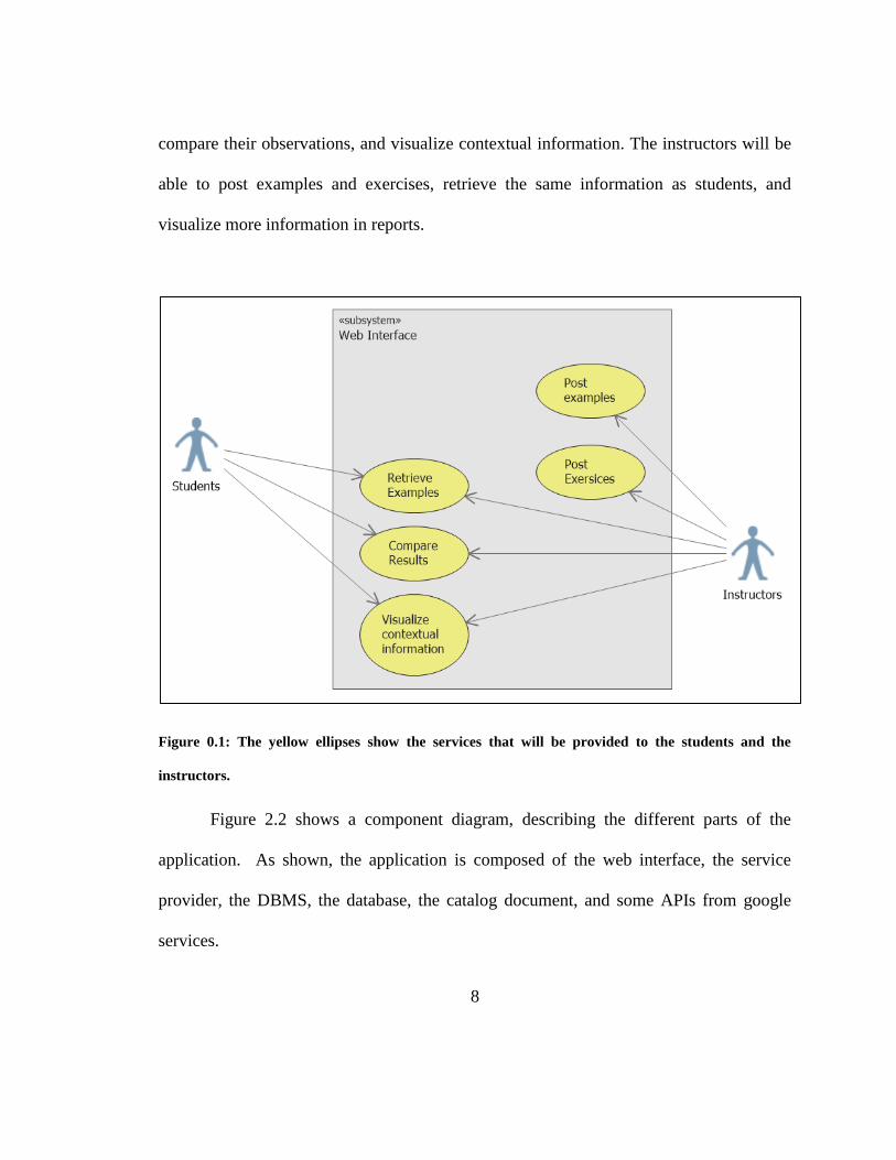
Figure 2.1 shows the use case diagram, describing the interaction of instructors and
students with the GEOWAPP interface. The students will be able to retrieve examples,
8
compare their observations, and visualize contextual information. The instructors will be
able to post examples and exercises, retrieve the same information as students, and
visualize more information in reports.
Figure 0.1: The yellow ellipses show the services that will be provided to the students and the
instructors.
Figure 2.2 shows a component diagram, describing the different parts of the
application. As shown, the application is composed of the web interface, the service
provider, the DBMS, the database, the catalog document, and some APIs from google
services.

9
Figure 0.2: This UML component diagram describes the GEOWAPP.
The service provider will be composed of three components: the requester, the
comparator, and the authoring tool. The requester will post the required information to the
DBMS system, which will retrieve data stored in the database or in text files. If a student
merely wants to see a layer, the GEOWAPP will display it on the interface. However, if
the student wants to compare his/her observations, this data will be sent to the comparator
10
tool. This tool will be able to compare stored data (samples) with the observed data,
producing an output that will inform to students about the accuracy of their observations.
This output will depend on the practical exercise that was assigned. In addition, the
authoring tool will provide instructors the ability to import new data into the database, such
as control points, bench marks, topographical features, and others.
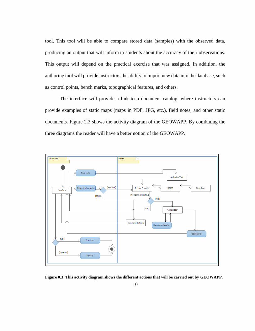
The interface will provide a link to a document catalog, where instructors can
provide examples of static maps (maps in PDF, JPG, etc.), field notes, and other static
documents. Figure 2.3 shows the activity diagram of the GEOWAPP. By combining the
three diagrams the reader will have a better notion of the GEOWAPP.
Figure 0.3 This activity diagram shows the different actions that will be carried out by GEOWAPP.

11
1.2 Exercises’ schemata
Sepehr (2009) states that the type of data as the reason for storing it in a geodatabase
must be specified before selecting any approach for implementing the geodatabase. In this
application, the field exercises will limit the data types. Therefore, these exercises must be
designed before either the database or any other component of the GEOWAPP.
Before designing the prototype exercises, the practicum courses must be studied.
These courses consist of GGE 1001(Introduction to Geodesy & Geomatics), GGE 1803
(Practicum for Civil Engineers), and GGE 2013 (Advance Survey Practicum).
1.2.1 Review of GGE’s field practices exercises
The outlines and labs of the GGE’s practicums have been reviewed in order to adapt
the GEOWAPP to what is already being taught. This review was organized by course. For
each course, a short description was written about which exercises could be included in the
GEOWAPP, and how the accuracies could be tested by a GEOWAPP.
1.2.1.1 GGE 1001 Introduction to Geodesy and Geomatics
This an introductory course for first-year students, coordinated by Dr. Peter Dare. Several
other GGE professors are also involved: Dr. Emmanuel Stefanakis, Dr. Marcelo Santos,
Dr. Yun Zhang, and Dr. John Hughes Clarke. Although this course is not a practical course
12
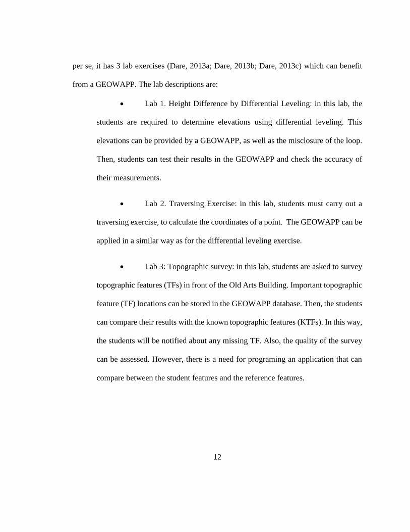
per se, it has 3 lab exercises (Dare, 2013a; Dare, 2013b; Dare, 2013c) which can benefit
from a GEOWAPP. The lab descriptions are:
Lab 1. Height Difference by Differential Leveling: in this lab, the
students are required to determine elevations using differential leveling. This
elevations can be provided by a GEOWAPP, as well as the misclosure of the loop.
Then, students can test their results in the GEOWAPP and check the accuracy of
their measurements.
Lab 2. Traversing Exercise: in this lab, students must carry out a
traversing exercise, to calculate the coordinates of a point. The GEOWAPP can be
applied in a similar way as for the differential leveling exercise.
Lab 3: Topographic survey: in this lab, students are asked to survey
topographic features (TFs) in front of the Old Arts Building. Important topographic
feature (TF) locations can be stored in the GEOWAPP database. Then, the students
can compare their results with the known topographic features (KTFs). In this way,
the students will be notified about any missing TF. Also, the quality of the survey
can be assessed. However, there is a need for programing an application that can
compare between the student features and the reference features.

13
1.2.1.2 GGE 1803 Practicum for Civil Engineers
This is a two week long course where the students develop their professional skill in field
surveying. The course is taught by Ryan White (Surveying) and Dave Fraser (GIS) (White
& Fraser, 2013). The GEOWAPP can assist with:
Traverse survey: after students have done the traverse exercise they
can check their accuracy in the GEOWAPP. The GEOWAPP can adjust the traverse
using the “Bowditch Rule”. Then, the students can check their results with the
calculated results made by the GEOWAPP.
Differential leveling: If a differential levelling network is done, the
application would apply network adjustments and the student would be able to
compare their result with the computed results of the GEOWAPP.
Topographic survey/map: A reference TIN can be stored in the
database. Then, when the students generates their own TIN the difference between
both of them can be reported. This report can have some advice and also can show
where points are needed or which place is over surveyed, depending on the
accuracy needed. However, there is a need to program an application that can
compare between the two TINs. Moreover, examples of topographic maps and of
corresponding field notes can be provided. Also, there is another method that can
be used to test the students’ observed ground points (SOGP). This method consists
of using the student’s observations for interpolating the z coordinate of the known

14
points. Then, the differences between the interpolated z coordinates and the known
z coordinates will give an indicator of the observation accuracy.
1.2.1.3 GGE 2013 Advanced Surveying Practicum.
Like the course GGE 1803, GGE 2013 is a two week long course. GGE 2013 is coordinated
by Dr. Dare and the Ph. D. student, Gozde Akay (Dare & Akay, 2014). This course is more
advanced than the previous two courses. However, the course can still be assisted as
described
Control network: The students are required to densify a local control
network within the work area using GPS. This densification must be carried out
using coordinates in the NAD83 (CSRS) system. This exercise can be supported by
adding control station coordinates to the GEOWAPP. Then, if there is a problem
during post processing or if the coordinates’ epoch is not correct, the application
can show students differences between the coordinates and advice on how to fix the
problem. This Control network requires also a survey of a traverse.
Topographic survey: Using the coordinate densification mentioned
before, students are asked to carry out a topographic survey of an indicated area
using a specified coding scheme. This exercise can be supported in two ways.
1. The method proposed for Lab 3 in GGE 1001 can be applied.
15
2. The TIN can be compared using the method proposed for the
course GGE 1803.
Heighting: The students are asked to determine heights of all the
points using GPS and/or differential leveling and/or vertical angle measurement to
local height benchmark. By programing an application tool, it would be possible to
measure the accuracy of the topographic network. For example, the least squares
method can be applied to a network, with redundant measurements. The application
can ask for 3 quantities: the distance between points, the vertical differences, and
the students’ computed values. Then, the application will report back the
differences between the students’ computed values and the GEOWAPP results.
Topographic plan: The students are asked to produce a topographic
plan of the area surveyed. The web mapping tool can provide links to good
examples of topographic maps done in the past, in order to guide students about
which map elements the map should contain.
In summary, the practicum exercises that will be supported by the GEOWAPP are
listed in table 2.1.

16
Table 0.1 Exercises classes classified by course
Exercises GEE 1001 GGE 1803 GGE 2013
Traversing X X X
Differential Leveling X X X
Topographic Survey X X X
Network densification X
Topographic plan X X X
1.2.1.4 Required Data
Table 2.2 shows the data required by each exercise to be implemented in the
GEOWAPP.
Table 0.2: Exercises classes classified by course
Exercises Data
Traversing Control points coordinates
Differential Leveling Benchmark heights
Topographic Survey Control points coordinates, TF with code, DTM (digital Terrain Model),
or KTF coordinates.
Network densification Coordinates of the control points
Topographic plan Map examples, map check-list
Examples Map examples, field notes examples, link to external sources, etc

17
1.3 How to Test Accuracies
One of the concerns of this research is to provide appropriate reports to students.
Then, instead of giving the signed differences, the GEOWAPP can retrieve an absolute
value of the differences. This approach is helpful in traversing exercises, differential
leveling exercises, and in the network densification. However, the topographic survey
exercises have different requirements.
A topographic plan is composed of representations of TFs and of relief. Thus, for
testing the accuracy of a topographic plan two different tools are required. As briefly
mentioned in Section 2.2, the vertical accuracies of the observations can be compared with
a TIN or with the interpolation computation previously discussed. Since summation of the
differences between the interpolated values in the TIN and the observations should tend to
0 if the observations are correct, some statistical tests can be applied in order to test the
accuracy of the vertical observations. This computation will be addressed in more detailed
in section 2.4 (vertical comparator). In the previous subsection, a spatial proximity tool
was mentioned, which will be able to compare the students’ observed topographic features
(SOTF) coordinates with the KTF coordinates, which are stored in the application. Also,
this will be addressed in section 2.4 (Proximity Comparator).
18
1.4 Required tools for testing accuracies
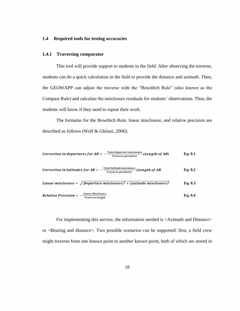
1.4.1 Traversing comparator
This tool will provide support to students in the field. After observing the traverse,
students can do a quick calculation in the field to provide the distance and azimuth. Then,
the GEOWAPP can adjust the traverse with the “Bowditch Rule” (also known as the
Compass Rule) and calculate the misclosure residuals for students’ observations. Thus, the
students will know if they need to repeat their work.
The formulas for the Bowditch Rule, linear misclosure, and relative precision are
described as follows (Wolf & Ghilani ,2006):
𝑪𝒐𝒓𝒓𝒆𝒄𝒕𝒊𝒐𝒏 𝒊𝒏 𝒅𝒆𝒑𝒂𝒓𝒕𝒖𝒓𝒆𝒔 𝒇𝒐𝒓 𝑨𝑩 = −𝑻𝒐𝒕𝒂𝒍 𝒅𝒆𝒑𝒂𝒓𝒕𝒖𝒓𝒆 𝒎𝒊𝒔𝒄𝒍𝒐𝒔𝒖𝒓𝒆
𝑻𝒓𝒂𝒗𝒆𝒓𝒔𝒆 𝒑𝒆𝒓𝒊𝒎𝒆𝒕𝒆𝒓𝒙𝑳𝒆𝒏𝒈𝒕𝒉 𝒐𝒇 𝑨𝑩) Eq. 0.1
𝑪𝒐𝒓𝒓𝒆𝒄𝒕𝒊𝒐𝒏 𝒊𝒏 𝒍𝒂𝒕𝒊𝒕𝒖𝒅𝒆𝒔 𝒇𝒐𝒓 𝑨𝑩 = −𝑻𝒐𝒕𝒂𝒍 𝒍𝒂𝒕𝒊𝒕𝒖𝒅𝒆 𝒎𝒊𝒔𝒄𝒍𝒐𝒔𝒖𝒓𝒆
𝑻𝒓𝒂𝒗𝒆𝒓𝒔𝒆 𝒑𝒆𝒓𝒊𝒎𝒆𝒕𝒆𝒓𝒙𝑳𝒆𝒏𝒈𝒕𝒉 𝒐𝒇 𝑨𝑩 Eq. 0.2
𝑳𝒊𝒏𝒆𝒂𝒓 𝒎𝒊𝒔𝒄𝒍𝒐𝒔𝒖𝒓𝒆 = √(𝑫𝒆𝒑𝒂𝒓𝒕𝒖𝒓𝒆 𝒎𝒊𝒔𝒄𝒍𝒐𝒔𝒖𝒓𝒆)𝟐 + (𝑳𝒂𝒕𝒊𝒕𝒖𝒅𝒆 𝒎𝒊𝒔𝒄𝒍𝒐𝒔𝒖𝒓𝒆)𝟐 Eq. 0.3
𝑹𝒆𝒍𝒂𝒕𝒊𝒗𝒆 𝑷𝒓𝒆𝒄𝒊𝒔𝒊𝒐𝒏 = −𝑳𝒊𝒏𝒆𝒂𝒓 𝑴𝒊𝒔𝒄𝒍𝒐𝒔𝒖𝒓𝒆
𝑻𝒓𝒂𝒗𝒆𝒓𝒔𝒆 𝒍𝒆𝒏𝒈𝒕𝒉 Eq. 0.4
For implementing this service, the information needed is <Azimuth and Distance>
or <Bearing and distance>. Two possible scenarios can be supported: first, a field crew
might traverse from one known point to another known point, both of which are stored in

19
the database. Second, a work team might start from an unknown point and perform a loop
traverse back to the same point.
The departures and the latitudes, which are the X and Y projections of the polar
coordinates of a vector are computed according to Eq. 2.5 and 2.6.
𝑫𝒆𝒑𝒂𝒓𝒕𝒖𝒓𝒆 = 𝑳𝒆𝒏𝒈𝒕𝒉 𝒐𝒇 𝑨𝑩 ∗ 𝒔𝒊𝒏 (𝑨𝒛𝒊𝒎𝒖𝒕𝒉 𝒇𝒓𝒐𝒎 𝑨 − 𝑩) Eq. 0.5
𝑳𝒂𝒕𝒊𝒕𝒖𝒅𝒆 = 𝑳𝒆𝒏𝒈𝒕𝒉 𝒐𝒇 𝑨𝑩 ∗ 𝒄𝒐𝒔(𝑨𝒛𝒊𝒎𝒖𝒕𝒉 𝒇𝒓𝒐𝒎 𝑨 − 𝑩) Eq. 0.6
(Wolf & Ghilani, 2006)
While the students are in the field, the most important information is the linear
misclosure, the residuals of latitude and departure, and the relative precision. However, the
full Bowditch rule report, shown in Table 3, can be used by the instructors to mark the
assignment.
An example of the schema of the students’ output is shown in Figure 2.4, using the
XML language.

20
Figure 0.4: This figure shows an example of the schema, which contains useful information for students
Table 0.3: Proposed format of the Bowditch rule report
Station Preliminary
Azimuths
Length
(m)
Unadjusted Balanced Coordinates
Departure Latitude Departure Latitude Eating Nothing
A XX XX
XXX XXX XX XX XX XX
B XX XX
XXX XXX XX XX XX XX
A XX XX
Sum XX XX 0 0
This format is taken from Wolf and Ghilani (2006). A full description of the Bowditch rule
is also given in their book. In addition, Milne (1984) shows a set of routines for computing
a traverse, which include the Bowditch adjustment (Compass Rule). These routines were
programmed in BASIC (Milne, 1984).
1.4.2 Leveling Tools
Differential leveling is a very precise method for determining the height
differences between objects. This methodology is found in a most surveying textbooks (e.g.
<residual of departure> 15 cm </ residual of departure >
<residual of latitude>7 cm</ residual of latitude >
<linear misclosure> 16.553 cm</ linear misclosure>
<traverse length>120 m</traverse length >
<relative precision>1 / 724.9485 < /relative precision >
<message>the traverse is off-tolerance</message >
21
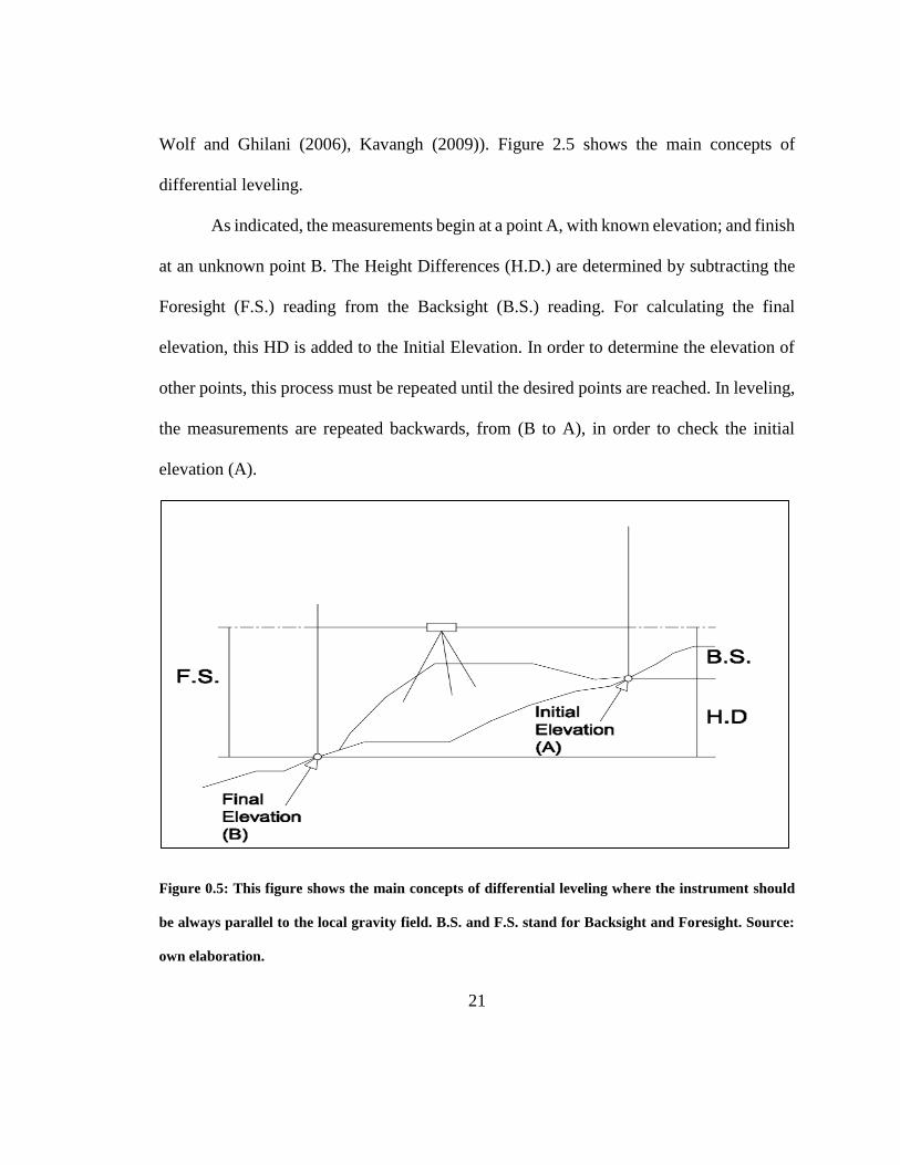
Wolf and Ghilani (2006), Kavangh (2009)). Figure 2.5 shows the main concepts of
differential leveling.
As indicated, the measurements begin at a point A, with known elevation; and finish
at an unknown point B. The Height Differences (H.D.) are determined by subtracting the
Foresight (F.S.) reading from the Backsight (B.S.) reading. For calculating the final
elevation, this HD is added to the Initial Elevation. In order to determine the elevation of
other points, this process must be repeated until the desired points are reached. In leveling,
the measurements are repeated backwards, from (B to A), in order to check the initial
elevation (A).
Figure 0.5: This figure shows the main concepts of differential leveling where the instrument should
be always parallel to the local gravity field. B.S. and F.S. stand for Backsight and Foresight. Source:
own elaboration.
22
In order to support this practice with the application, the GEOWAPP provides two
options:
1.4.2.1 Leveling Comparator
The height difference will be known by the GEOWAPP because the control points
will be stored in the database. The students can then post their measured height difference,
and the tool can reply to indicate whether the measurements are within a tolerance specified
by the instructor. This will be done by comparing the computed H.D. and the stored H.D.
The whole computation can be carried out by the GEOWAPP, and absolute values of
residuals can be shown as well as the precision. The precision of leveling is computed with
the following formula.
𝑪 = 𝒎√𝑲 Eq. 0.7
where:
C is the misclosure in mm,
m is a constant to be compared with the standard of precision, and
K is the perimeter of the leveling, which is distance between point A and B
multiplied by 2, in kilometers.

23
Figure 2.6 shows the schema definition of the information that will be retrieved
from GEOWAPP.
Figure 0.6 shows the students report schema for the differential leveling.
The orders of accuracy are specified in the outline of GGE 1803: Practicum for
Civil Engineers, and are also shown in Table 2.4.
1.4.2.2 Leveling Least Squares Checking
For advanced surveying students, a leveling network is generated and a least
squares adjustment can be performed. In this case, a measurement of the students’
observation accuracy is given by the statistics of the adjustment (mean, standard deviation,
and variance). This adjustment method in Wolf & Ghilani (1997), Wolf & Ghilani (2006).
However, there are a huge amount of literature about the least square adjustment.
<misclosure> 0.030 m</misclosure>
<distance>0.300 km</distance>
<perimeter>0.600 km </perimeter>
<m>0.38730</m >
<order of accuracy>Fourth order < / order of accuracy>
<message>the accuracy is insufficient</message >
24
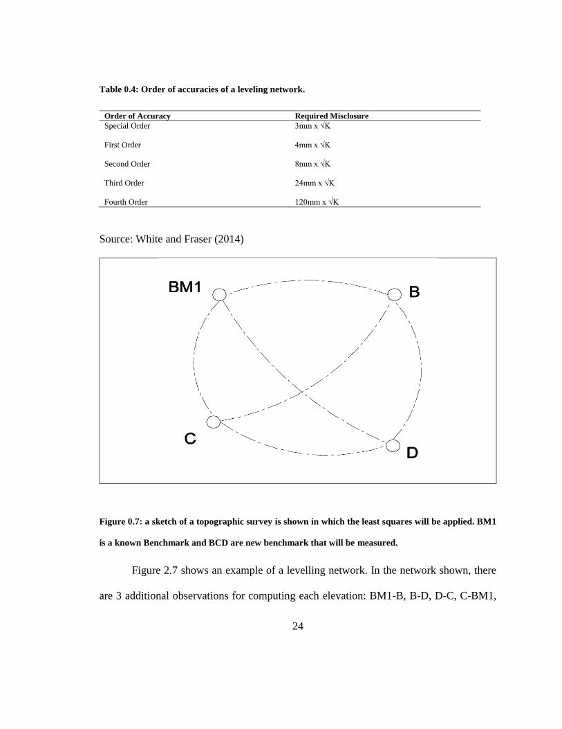
Table 0.4: Order of accuracies of a leveling network.
Order of Accuracy Required Misclosure
Special Order 3mm x √K
First Order 4mm x √K
Second Order 8mm x √K
Third Order 24mm x √K
Fourth Order 120mm x √K
Source: White and Fraser (2014)
Figure 0.7: a sketch of a topographic survey is shown in which the least squares will be applied. BM1
is a known Benchmark and BCD are new benchmark that will be measured.
Figure 2.7 shows an example of a levelling network. In the network shown, there
are 3 additional observations for computing each elevation: BM1-B, B-D, D-C, C-BM1,
25
BM1-D, and B-C. Thus, a least squares adjustment can be applied. The formula for
computing the final values is:
𝑿 = (𝑨𝑻𝑾𝑨)−𝟏(𝑨𝑻𝑾𝑳) Eq. 0.8
where:
X is the matrix of unknowns,
A is the matrix of coefficients,
L is the matrix of observations, and
W is the matrix of weights.
(Wolf & Ghilani, 2006)
The matrix of weights in leveling is usually a diagonal matrix, composed of the
inverse of the distances between benchmarks.
The Residual matrix b (𝑉) is calculated according to Eq. 2.9.
𝑽 = 𝑨𝑿 − 𝑳 Eq. 0.9
(Wolf & Ghilani, 2006)
In addition, the standard deviation is computed according to Eq. 2.10 and Eq. 2.11.
𝝈𝟎 = √𝑽𝑻𝑾𝑽
𝒓 Eq. 0.10
and
𝝈𝒙𝒊= 𝝈𝟎√𝒒𝒙𝒊𝒙𝒊 Eq. 0.11

26
where:
𝜎0 is the standard deviation of unit weight,
𝑟 is the degrees of freedom,
𝑞𝑥𝑖𝑥𝑖 is the diagonal values of matrix (𝐴𝑇𝑊𝐴)−1, and
𝜎𝑥𝑖 is the standard deviation of the adjusted value.
(Wolf & Ghilani, 2006)
After applying this method, a report can be given to students. This report is
described as follows (see Figure 2.8).
Figure 0.8: this figure shows the schema definition of the students report using the Leveling Least
Squares Checking tool.
<residual 1>0.001 m </ residual 1>
…
<residual n>0.003 m </ residual n>
<distance 1>0.300 km</distance 1>
…
<distance n>0.200 km</distance n>
<elevation 1>10000.000m </elevation 1>
<st. dv. 1>0.002 m</ st. dv. 1>
...
<elevation n>10099.531m </elevation n>
<st. dv. n>0.004 m</ st. dv. n>
<message>the accuracy is enough</message >
27
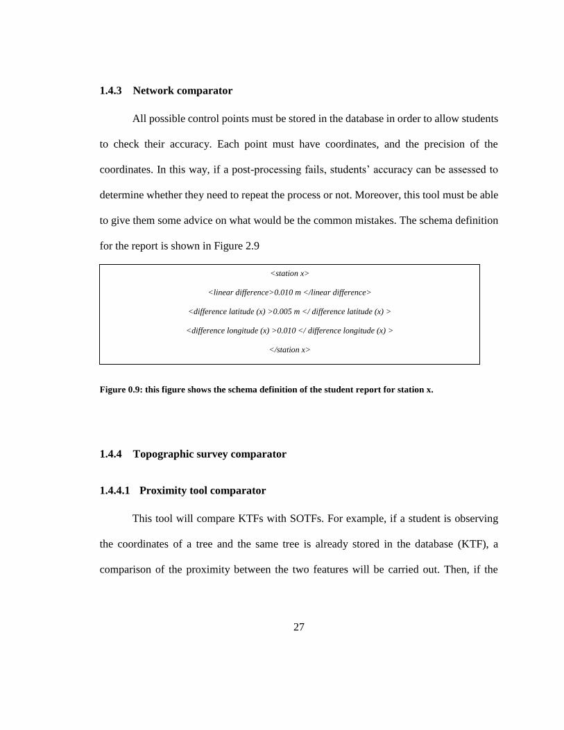
1.4.3 Network comparator
All possible control points must be stored in the database in order to allow students
to check their accuracy. Each point must have coordinates, and the precision of the
coordinates. In this way, if a post-processing fails, students’ accuracy can be assessed to
determine whether they need to repeat the process or not. Moreover, this tool must be able
to give them some advice on what would be the common mistakes. The schema definition
for the report is shown in Figure 2.9
Figure 0.9: this figure shows the schema definition of the student report for station x.
1.4.4 Topographic survey comparator
1.4.4.1 Proximity tool comparator
This tool will compare KTFs with SOTFs. For example, if a student is observing
the coordinates of a tree and the same tree is already stored in the database (KTF), a
comparison of the proximity between the two features will be carried out. Then, if the
<station x>
<linear difference>0.010 m </linear difference>
<difference latitude (x) >0.005 m </ difference latitude (x) >
<difference longitude (x) >0.010 </ difference longitude (x) >
</station x>
28
feature is within the tolerance, it will be accepted. If the feature is not within the tolerance,
it will be marked as outlier.
The above mentioned check requires that each TF be encoded, as done by Sepher
(2009). These codes are shown in Table 2.5. Tolerances for each feature, however, must
be defined in this research.
In order to define the tolerances, the errors in the measurements have to be
analyzed. Nickerson (1978) wrote a report about the different errors found in surveying
observations. These errors can be divided into internal and external: internal errors are
related with the equipment itself while external errors are related with the environment.
For this application, the correction for environmental conditions, like temperature and
humidity, and systematic errors are assumed to be already accounted by students. Besides,
the analysis of every measurement would not be feasible for the proposed application;
however, a common internal error will be derived from Nickerson’s formulas.

29
Table 0.5: Specification of the code system for the survey practicums.
New feature coding system Feature type Students’ feature codes
BL Buildings · Buildings · BLD
BN Benches · Benches BR Bike racks · Benches&Bikerack Contours Contour lines · Contours CB Curbs · Curb
· Top of curb ·Curbs&walkways&sidewalk
EB Electrical boxes · Electrical box FN Fences · Fence GF Green fields · Vegetation HD Hydrants · Hydrant
·Manholes&Firehydr&sign LI Lights · Light LP Lamp posts · Lamp Post
Tree&Post
MH Manholes Manholes&Firehydr&sign PG Play grounds - PL Parking areas · Parking Lot SI Signs · Sign
· Signs ST Streets · Asphalt
· Road · Road&Sidewalk
SD Storm drains · Storm Drain SW Sidewalks or any type of walkways · Sidewalk
· Road&Sidewalk ·Curbs&walkways&sidewalk
WA Treed or wooded areas · Woods · Tree Line
TR Trees · Vegetation · Tree · Tree&Post
RW Retaining Walls · Retaining Wall · RWALL
TP Telephone poles · Telephone poles
Source: (Sepehr, 2009)
In angular observations, Nickerson (1978) states that there are three different
internal errors (𝜎𝑖): pointing error(𝜎𝑝), reading error (𝜎𝑟), leveling error(𝜎𝐿) (see Eq. 2.12).
These are related according to (Nickerson, 1978):

30
𝝈𝒊𝟐 = 𝝈𝒑
𝟐 + 𝝈𝒓𝟐 + 𝝈𝑳
𝟐 Eq. 0.12
Table 0.6: Acceptable internal error for different classes of survey
Order of survey Order of class Nominal Relative accuracy
Internal Error.
1 1:100 000 0”. 33
2 1 1: 50 000 0”. 33
2 2 1:20 000 0”.47
3 1 1: 10 000 0”.69
3 2 1: 5 000 1”.39
Source: Pfeifer (1975) as cited by Nickerson (1978)
These internal errors are meant for experienced observer, who will ensure that the
equipment is set up correctly. As students are learning how to measure and setting up, the
internal error (σ𝑖) can be greater than σ𝑖 that would be made by an experienced observer.
In addition to angular errors, the distance measuring error has to be taken into
account. For mapping topographical features, EDMs (electronic distance measuring
instruments) are used in the survey practicums. These instruments have built-in errors,
although McCormac et al. (2013) state that “Instrument errors are usually quite small if the
equipment has been carefully adjusted and calibrated”. In addition, McCormac, et al.
(2013) states that the EDMs manufacturers give an instrument constant for the built-in
error, which is called instrumental error (IE); and another value that is dependent on the
31
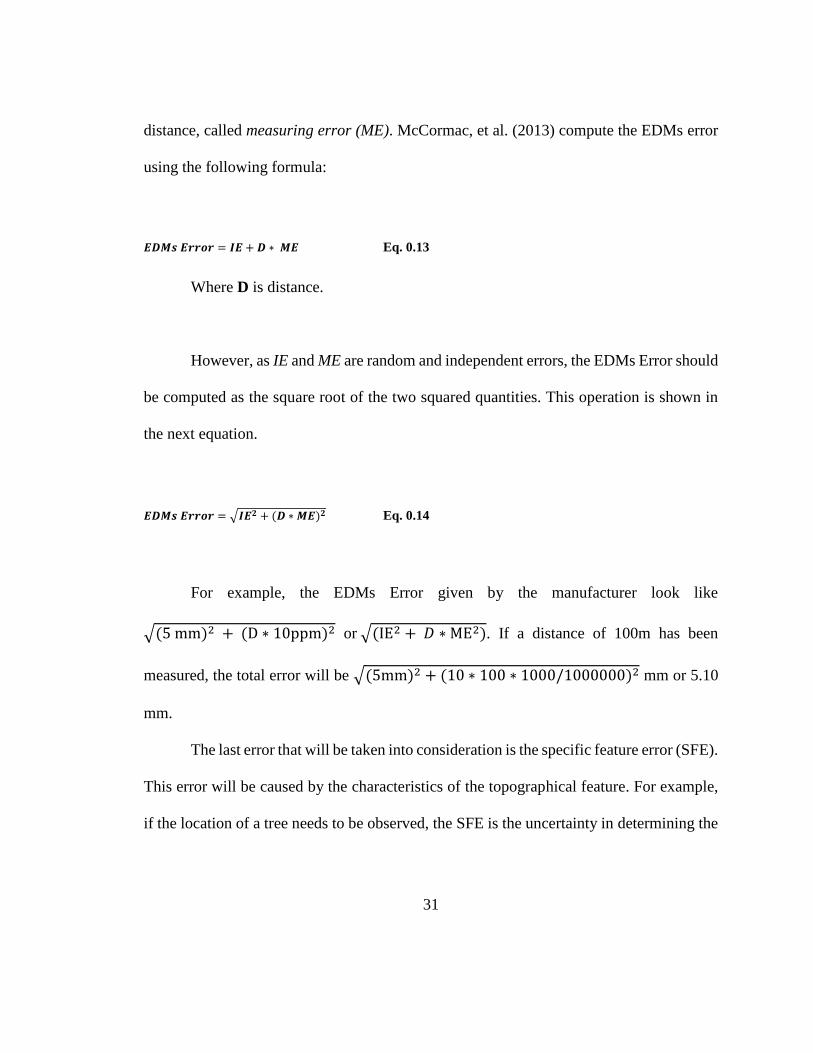
distance, called measuring error (ME). McCormac, et al. (2013) compute the EDMs error
using the following formula:
𝑬𝑫𝑴𝒔 𝑬𝒓𝒓𝒐𝒓 = 𝑰𝑬 + 𝑫 ∗ 𝑴𝑬 Eq. 0.13
Where D is distance.
However, as IE and ME are random and independent errors, the EDMs Error should
be computed as the square root of the two squared quantities. This operation is shown in
the next equation.
𝑬𝑫𝑴𝒔 𝑬𝒓𝒓𝒐𝒓 = √𝑰𝑬𝟐 + (𝑫 ∗ 𝑴𝑬)𝟐 Eq. 0.14
For example, the EDMs Error given by the manufacturer look like
√(5 mm)2 + (D ∗ 10ppm)2 or √(IE2 + 𝐷 ∗ ME2). If a distance of 100m has been
measured, the total error will be √(5mm)2 + (10 ∗ 100 ∗ 1000/1000000)2 mm or 5.10
mm.
The last error that will be taken into consideration is the specific feature error (SFE).
This error will be caused by the characteristics of the topographical feature. For example,
if the location of a tree needs to be observed, the SFE is the uncertainty in determining the

32
location of the tree center. For the purposes of this project, the expertise of the instructor
will be used to determine these values.
Merging the three errors together, the tolerance of TFs are define. Normally, an
Elliptical Error Probable (EEP) should be defined because of the propagation of the errors.
This concept is shown in Figure 2.10.
Figure 0.10: The EDMs error propagates along line of sight from the observer while σi (radians)
propagates across the line of sight; . The SFE is added to both errors (EDMs error and σi).
However, because the position of the observer is hard to locate in a student’s observation
coordinate file, then a Circular Probable Error (CPE) can be computed instead of an EEP.
The formula for computing the 50% CPE is shown next.
𝑹 = 𝟎. 𝟕𝟓 ∗ √(𝑬𝑷𝑷 𝑴𝒊𝒏𝒐𝒓 𝑨𝒙𝒊𝒔 )𝟐 + (𝑬𝑷𝑷 𝑴𝒂𝒚𝒐𝒓 𝑨𝒙𝒊𝒔 )𝟐 Eq. 0.15

33
Source: (Mathematical Analysis and Research Corp., 1987)
The Mathematical Analysis and Research Corp. (1987) demonstrated the
relationship between the confidence level of the EEP and the CPE for two extreme cases,
when an EEP is circular and when an EPP is highly skewed. For example, if a CPE is
derived from a 95 % EEP, this CPE confidence level will vary between the value of 93 %
and 97 %.
A confidence level of 99 % is taken as standard for accepting or rejecting a
measurement. Expansion factor can be derived from the Normal distribution. This
expansion factor for 99% is approximately 3.035.
The 99% CPE can be derived from a 99% EEP by using Eq. 2.15 and the
corresponded expansion factor. The formula is shown next.
𝑹 = 𝟎. 𝟕𝟓 ∗ 𝟑. 𝟎𝟑𝟓 ∗ √[√(𝑫 ∗ 𝝈𝒊𝟐 + 𝑺𝑭𝑬𝟐) ]𝟐 + [√(𝑬𝑫𝑴𝒔 𝑬𝒓𝒓𝒐𝒓𝟐 + 𝑺𝑭𝑬𝟐) ]𝟐 Eq. 0.16
Then, the confidence level from this CPE vary between 99.5% and 97.3%, derived
from Mathematical Analysis and Research Corp. (1987). Then, our tolerance will be
defined as R. The concept of this tolerance can be represented graphically as in Figure 2.11.
34
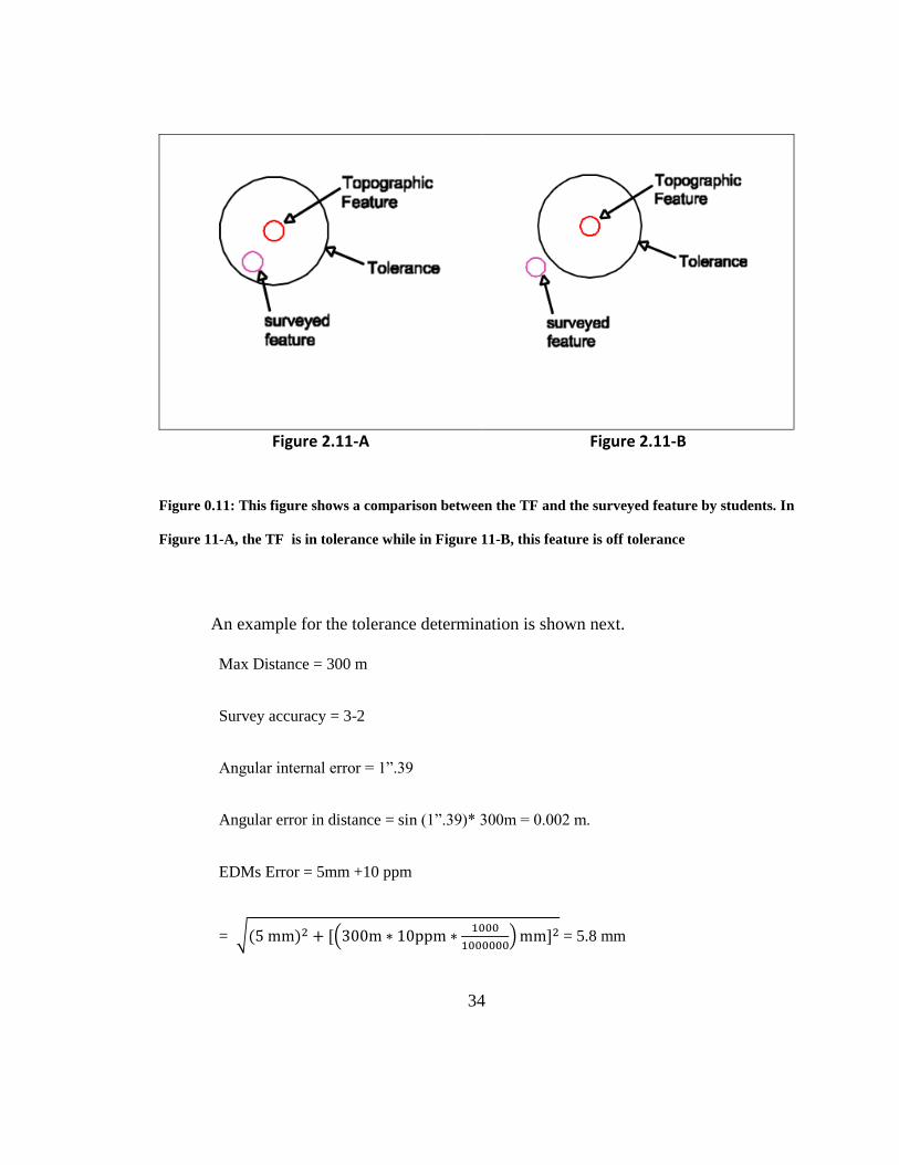
Figure 2.11-A Figure 2.11-B
Figure 0.11: This figure shows a comparison between the TF and the surveyed feature by students. In
Figure 11-A, the TF is in tolerance while in Figure 11-B, this feature is off tolerance
An example for the tolerance determination is shown next.
Max Distance = 300 m
Survey accuracy = 3-2
Angular internal error = 1”.39
Angular error in distance = sin (1”.39)* 300m = 0.002 m.
EDMs Error = 5mm +10 ppm
= √(5 mm)2 + [(300m ∗ 10ppm ∗1000
1000000) mm]2 = 5.8 mm
35
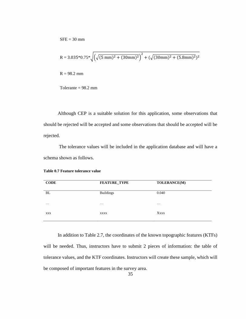
SFE = 30 mm
R = 3.035*0.75*√(√(5 mm)2 + (30mm)2)2
+ (√(30mm)2 + (5.8mm)2)2
R = 98.2 mm
Tolerante = 98.2 mm
Although CEP is a suitable solution for this application, some observations that
should be rejected will be accepted and some observations that should be accepted will be
rejected.
The tolerance values will be included in the application database and will have a
schema shown as follows.
Table 0.7 Feature tolerance value
CODE FEATURE_TYPE TOLERANCE(M)
BL Buildings 0.040
… … …
xxx xxxx Xxxx
In addition to Table 2.7, the coordinates of the known topographic features (KTFs)
will be needed. Thus, instructors have to submit 2 pieces of information: the table of
tolerance values, and the KTF coordinates. Instructors will create these sample, which will
be composed of important features in the survey area.

36
1.4.4.2 Vertical tool comparator
The main purpose of this tool is to determine whether the students’ survey meets the
requirements of the exercise. In spatial data, the only way to confirm that these
requirements are met are statistical tests at moderate cost (Aguilar, Aguilar, & Aguera,
2007). Hohle and Holhe (2009) state that the accuracy of measurements in a DTM are
usually based in the assumption that the errors follow a Gaussian distribution, and that no
outliers exist. Often this is not true. Their research was based on DTMs derived by
Photogrammetry and Remote Sensing. These authors further underline the fact that there
may be some unwanted objects (Ex. cars, buildings and people), which may cause that
some of the ground points to be incorrectly labeled. These unwanted objects will not be
present in SOGPs, which will be generated during their exercises, because students will be
able to pick their ground points (GP) and label them correctly. Such GPs, which are
surveyed with total stations, have been used to measure accuracies of DEM in previous
studies (Gil et al., 2013; Reutebuch et al., 2000). Because of this advantage of SOGPs, it
can be assumed that their errors follow a Gaussian distribution. As result, common
statistical accuracy measures can be used: 𝜎 (Standard Deviation), 𝑅𝑀𝑆𝐸 (Root Mean
Square Error), �̅� (Mean Error). Furthermore, the Standard Normal Distribution and
Student’s t Distribution can be used for creating confidence intervals, depending whether
population or sample quantities are used. These statistical measures were suggested by
Holhe and Holhe (2009) when the Gaussian distribution requirement is met. Table 2.8
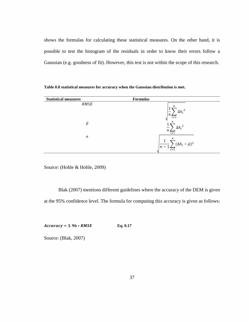
37
shows the formulas for calculating these statistical measures. On the other hand, it is
possible to test the histogram of the residuals in order to know their errors follow a
Gaussian (e.g. goodness of fit). However, this test is not within the scope of this research.
Table 0.8 statistical measures for accuracy when the Gaussian distribution is met.
Statistical measures Formulas
𝑅𝑀𝑆𝐸
√1
𝑛∑ ∆ℎ𝑖
2
𝑛
𝑖=1
�̅� 1
𝑛∑ ∆ℎ𝑖
2
𝑛
𝑖=1
𝜎
√1
𝑛 − 1∑(∆ℎ𝑖 − �̅�)2
𝑛
𝑖=1
Source: (Hohle & Hohle, 2009)
Blak (2007) mentions different guidelines where the accuracy of the DEM is given
at the 95% confidence level. The formula for computing this accuracy is given as follows:
𝑨𝒄𝒄𝒖𝒓𝒂𝒄𝒚 ≈ 𝟏. 𝟗𝟔 ∗ 𝑹𝑴𝑺𝑬 Eq. 0.17
Source: (Blak, 2007)
38
This vertical comparator can be developed using different approaches. These
approaches are discussed next.
1.4.4.2.1 Known points coordinates stored in the database or in a text file
This approach will require storage of some known point coordinates in the database
or in a text file, and uploading of DEM or TIN models already created. The GEOWAPP
will make a comparison between the known points coordinates and the DEM or TIN, and
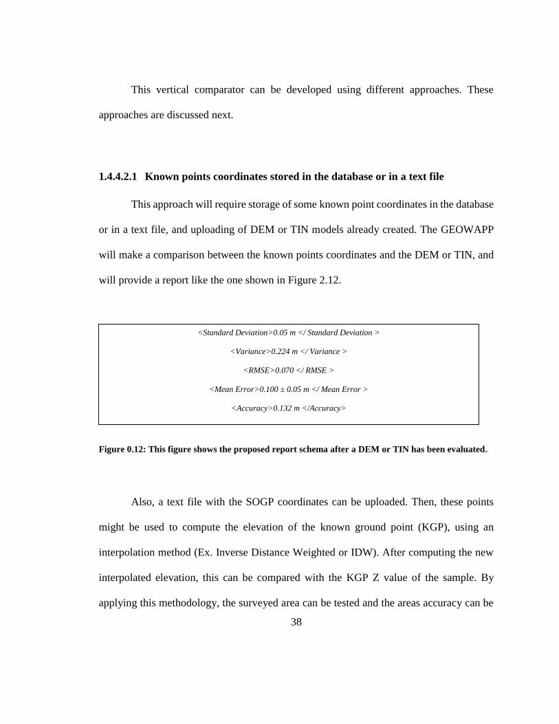
will provide a report like the one shown in Figure 2.12.
Figure 0.12: This figure shows the proposed report schema after a DEM or TIN has been evaluated.
Also, a text file with the SOGP coordinates can be uploaded. Then, these points
might be used to compute the elevation of the known ground point (KGP), using an
interpolation method (Ex. Inverse Distance Weighted or IDW). After computing the new
interpolated elevation, this can be compared with the KGP Z value of the sample. By
applying this methodology, the surveyed area can be tested and the areas accuracy can be
<Standard Deviation>0.05 m </ Standard Deviation >
<Variance>0.224 m </ Variance >
<RMSE>0.070 </ RMSE >
<Mean Error>0.100 ± 0.05 m </ Mean Error >
<Accuracy>0.132 m </Accuracy>

39
shown in a map. This method reduces the complexity of the programing part of this
research.
1.4.4.2.2 TIN stored in the application
With this approach, a TIN will be stored the applictaion, and students will upload
their SOGP. Then, the GEOWAPP will reply with a similar report than shown in Figure
2.12. However, an outlier evaluator function can be developed.
Outliers are values that cannot be considered as a part of a particular population
from a statistical point of view (Aguilar et al., 2007), while blunders are mistakes or gross
errors (Wolf & Ghilani, 1997). Wolf and Ghilani (1997) use these terms as synonyms when
comes to detecting them. In this research, “blunder” and “outlier” are used as synonyms
because these two concepts have too much in common while just looking at the data and
since our main purpose is detecting them. If blunders are present, this may be for different
reasons: the total station might be malfunctioning; the total station might be erroneously
set up; the prism pole might be incorrectly set up in the total station; or the student might
categorize a point incorrectly. For example, a point that belongs to an artificial structure
might be stored like a GP for generating a DTM.
Blak (2007) states that “a potential blunder may be identified as any error greater
than three times the standard deviation (3 sigma) of the error”. This author states also that
any check point with a large error should not be discarded without a proper investigation.
40
Blak also states that for determining vertical accuracy, the check points should be
acquired with a method that allows at least 3 times better accuracy than the DEM. This
requirement can be used with another approach. If a reference DEM has been determined
to have an accuracy X, and new measurements are added with an accuracy Y, these new
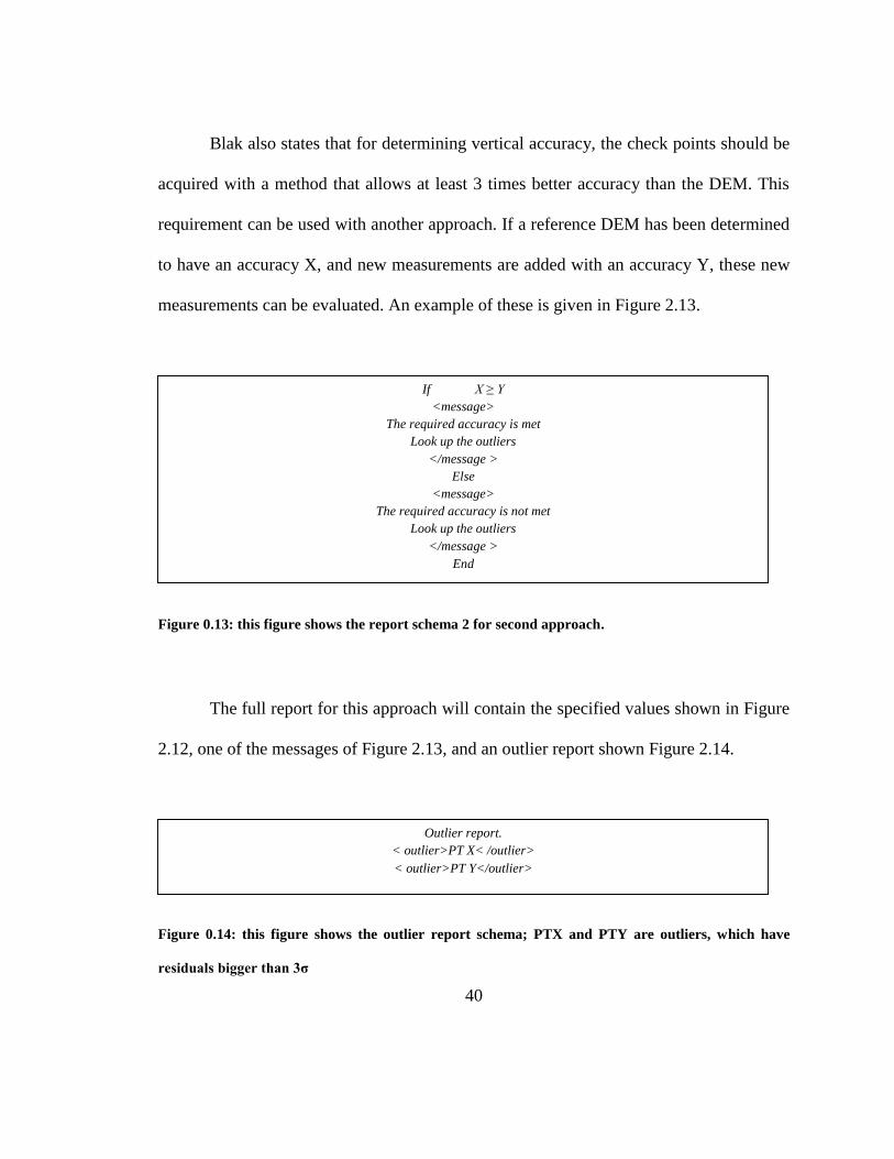
measurements can be evaluated. An example of these is given in Figure 2.13.
Figure 0.13: this figure shows the report schema 2 for second approach.
The full report for this approach will contain the specified values shown in Figure
2.12, one of the messages of Figure 2.13, and an outlier report shown Figure 2.14.
Figure 0.14: this figure shows the outlier report schema; PTX and PTY are outliers, which have
residuals bigger than 3σ
If X ≥ Y
<message>
The required accuracy is met
Look up the outliers
</message >
Else
<message>
The required accuracy is not met
Look up the outliers
</message >
End
Outlier report.
< outlier>PT X< /outlier>
< outlier>PT Y</outlier>
41
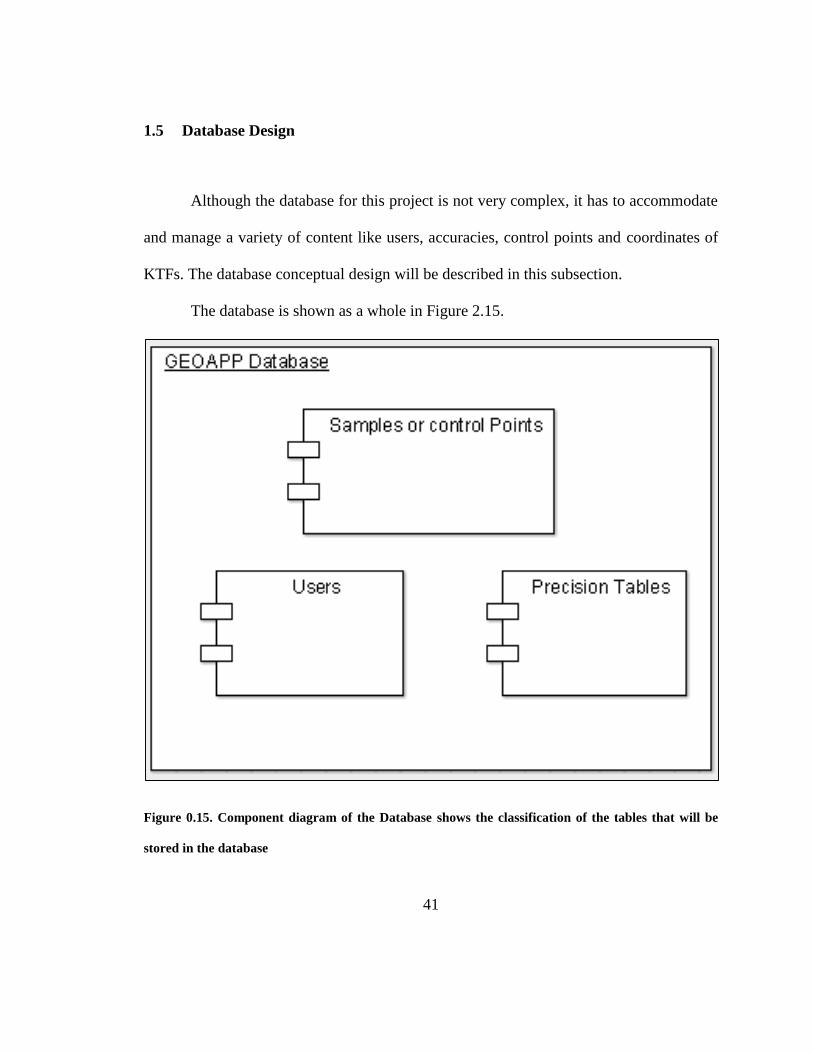
1.5 Database Design
Although the database for this project is not very complex, it has to accommodate
and manage a variety of content like users, accuracies, control points and coordinates of
KTFs. The database conceptual design will be described in this subsection.
The database is shown as a whole in Figure 2.15.
Figure 0.15. Component diagram of the Database shows the classification of the tables that will be
stored in the database

42
The sample and control points will include bench marks, GP, TF, etc. However,
when dealing with samples lists like KGP and KTF can also be stored in txt files. The user
table will store people who have a specific role: Administrators (Instructors, Teaching
Assistants) or Users (Students). Finally, the precision table will have an important role
because will set the requirements evaluating the students’ work. The table schema will be
discussed in the next chapter.
1.6 Authoring tool
The authoring tool will be limited in this research to the task of inserting new data
into the Database, as well as uploading new files in order to process the data. However,
this option will give freedom to choose new places to hold the survey practicums.
The next chapter will treat the application implementation, including the different
technologies that will be used and specific details about the application development. Also,
interaction between systems and some results will be shown.

43
Chapter 3: GEOWAPP prototype development
A GEOWAPP prototype was created to implement the idea developed in Chapter
2. This chapter provides an explanation of the different roles of technologies and
algorithms were created for the GEOWAPP. In order to create a web application that
processes data, several technologies should be combined. In this instance, technologies like
HTML, JavaScript, JQuery, PHP, MySQL, and Python were used to create the GEOWAPP
application. Bootstrap was added in order to improve the web application appearance and
responsiveness. Table 3.1 shows the technologies used and their role in the application.

44
Table 0.1: Technologies and functionality
Technology Function in the GEOWAPP
HTML Standard language.
JQuery, JavaScript Managing the contents of the Web interphase: load forms,
posting forms, display Google Maps, Display KMLs, etc.
PHP Creating dynamic forms, formatting information for Python
processing, and leveling and traversing processing
MySQL Managing the user’s tables, accuracy tables, code tables.
Python Vertical accuracy processing and horizontal accuracy
processing, creating the KML components.
Bootstrap Web appearance and responsivity
There are many important considerations while developing a software such as
technologies and their role, algorithms, libraries, other applications, physical structure
(folder and files), etc. the GEOWAPP physical structure shows the organization of the files
that compose the application.
1.7 Application Structure
The GEOWAPP is composed of various independent files. The first file is the
index.php, which basically provides the interphase of the web application. Then, the

45
application contains 11 folders, which are Forms, PHPS, CSS, fonts, REPORTS, Python,
uploads, img, js, and KMLS (see Figure 3.1). Every folder’s role is explained next.
Figure 0.1: application folders.
1.7.1 Forms
The Forms folder hosts all forms that are not dynamic. In other words, the forms in
this folder do not depend on the information that is provided by the user. Figure 3.2 shows
the form for traversing checking, called form_traverse_type.php.
46
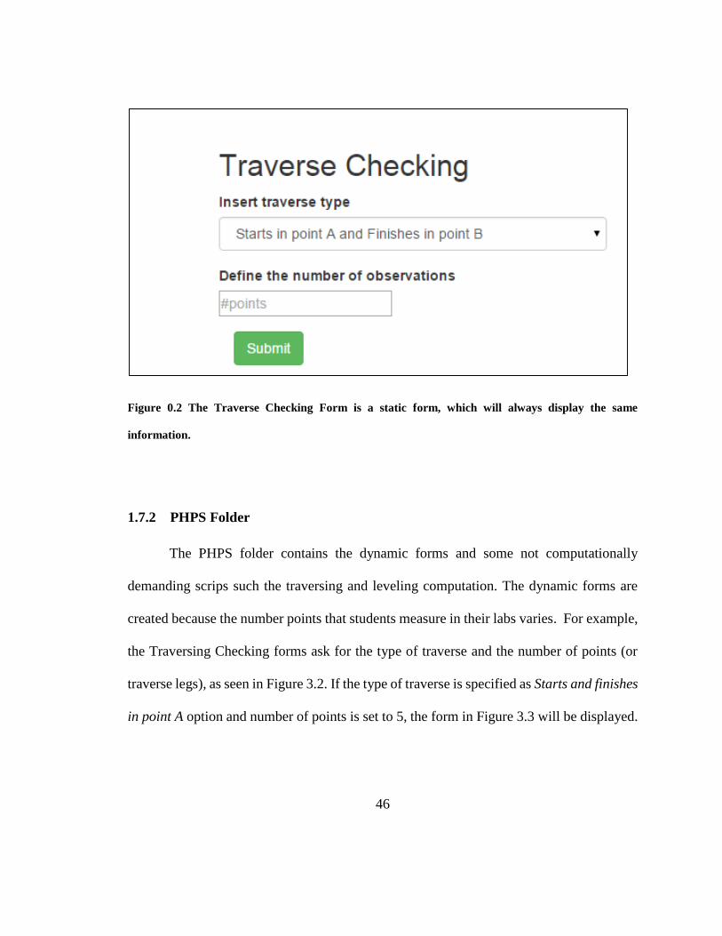
Figure 0.2 The Traverse Checking Form is a static form, which will always display the same
information.
1.7.2 PHPS Folder
The PHPS folder contains the dynamic forms and some not computationally
demanding scrips such the traversing and leveling computation. The dynamic forms are
created because the number points that students measure in their labs varies. For example,
the Traversing Checking forms ask for the type of traverse and the number of points (or
traverse legs), as seen in Figure 3.2. If the type of traverse is specified as Starts and finishes
in point A option and number of points is set to 5, the form in Figure 3.3 will be displayed.

47
Figure 0.3: This figure shows a form generated dynamically for the traversing checking. If the input
values vary in the previous form (Figure 3.2), this form will vary as well.
For traversing checking and leveling differential level checking, the computations
are done using a PHP script that is contained in the PHP folder. However, Python is used
for a computation that requires a use of matrices and/or elaboration of KML files. In such
a case, these PHP scripts just format the information for Python processing. This interaction
will be explained later when in this chapter every tool is described.
48
1.7.3 CSS, fonts, and JS folders
These folders store scripts for formatting and managing contents of the Web
application. For example, Js folder contains the library for JavaScript like JQuery, and
bootstrap and other plugin. CSS and fonts folders are components of the bootstrap
framework.
1.7.4 REPORTS, img, uploads folders, and KMLS
These folders contain different files such as images, text files, and KMLS. The
REPORT and KMLS folder store files that were built by the GEOWAPP, processed by
Python scripts. On the other hand, uploads folder contains two types of information:
samples files (KGP, KTF), which are uploaded for instructors, and students’ files, which
are the observations for testing. The Img folder contains images like the UNB logo or any
other image.
1.7.5 Python Folder
Python scripts are stored in this folder. These scripts carry out the heavy
computational part of the application like the Vertical Comparator and Proximity
Comparator. The descriptions of the Python algorithms are given in the discussion of each
corresponding tool in Section 3.3. Next, the GEOWAPP interface is described.

49
1.8 The GEOWAPP interface (Index.php )
The Index.php structure is composed of two (2) components: JavaScript or JQuery
functions and the user interface. Including content managing functions in Index.php makes
the interaction of such an application easier and more understandable. For instance, having
functions to load the forms in Index.php is more organized than loading the forms as
objects. In this way, all CSS styles are maintained and can be easily passed to other forms.
An example of a loading function is shown in Figure 3.4. A web application interface
similar to desktop applications is possible using JavaScript. More details about this ability
are not given because this is beyond of the scope of this research. Nevertheless, a brief
description is treated next.
Figure 0.4: this figure shows the loading function, which calls the form displayer and loads the traverse
form into the file.
The JS functions in Index.php are divided into two classes; (a) the content manager
displays, writes, and posts results in text form; (b) the Google Maps manager displays the
results on Google Maps. The next component, user interface, is also divided into two: the
navigation bar, and main window. While in the navigation bar users call the functions for
processing data and registering, they see the results in the main window. A logical schema
50
explaining Index.php is provided in Figure 3.5. Users will mainly interact with two
components of the interface: the toolbar and the form/results displayer.
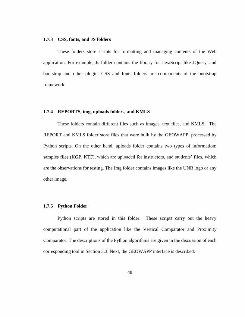
Figure 0.5 the xml schema shows the structure of the GEOWAPP interface. There are two classes of
functions: for managing the interface contents and for managing the Google Maps API. Then, there
are two main components in the user interface: the tool bar and the results displayer.
<GEOWAPP interface>
<Functions>
<content manager/>
<Google Maps manager/>
</Functions>
<user interface>
<navigation bar>
<registry bar>
<Tool bar/>
</navigation bar>
<main window>
<results displayer>
<computational results/>
<map results/>
</results displayer>
</main window>
</user interface>
</GEOWAPP interface>

51
Responsiveness allows web applications to have good organization and appearance
of information in different devices like cellphone, tables, or computers. The Bootstrap
framework were used to add responsiveness to GEOWAPP. Figure 3.6 and Figure 3.7
show different views of the GEOAWAPP depending on the screen resolution.
Figure 0.6: this figure shows the appearance of the GEOWAPP in large screens.
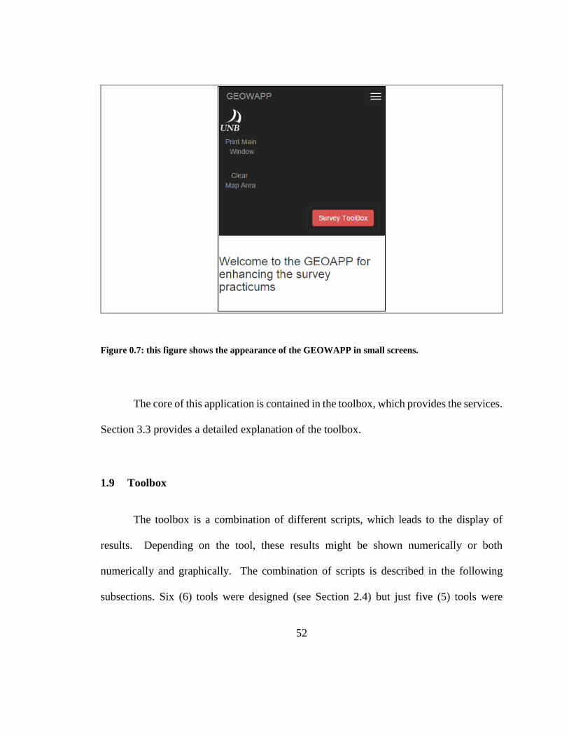
52
Figure 0.7: this figure shows the appearance of the GEOWAPP in small screens.
The core of this application is contained in the toolbox, which provides the services.
Section 3.3 provides a detailed explanation of the toolbox.
1.9 Toolbox
The toolbox is a combination of different scripts, which leads to the display of
results. Depending on the tool, these results might be shown numerically or both
numerically and graphically. The combination of scripts is described in the following
subsections. Six (6) tools were designed (see Section 2.4) but just five (5) tools were

53
developed (Traversing Comparator, Leveling Comparator, Leveling Network Comparator,
Proximity Comparator, Vertical Comparator). The Network Comparator was not
developed because the prototype’s purpose is to test the idea of the web application. Then,
the five (5) tools were enough for this purpose. However, the idea may be considered in
future research, and then, it is worth to have this tool mentioned in this document. Four (4)
out of five (5) tools use MySQL for storing required data. A database management system
is an important component in most of the applications. the description of the tools includes
the way MySQL is used and Section 3.3.6 shows the tables’ schemata.
1.9.1 Traversing Comparator
Traversing Comparator was developed as specified in Section 2.4. As shown in
Figure 3.2, the first forms ask for the type of traverse and for the number of points in a
traverse. The traverse type either (a) starts and finishes in different stations or (b) starts
and finishes in the same station. These two (2) options are graphically shown in Figure 3.8
and Figure 3.9, respectively. These two (2) figures display a traverse synthetically
generated with Matlab. After submitting the information, the application creates another
form, where students can insert distances and azimuths (See Figure 3.2).

54
Figure 0.8: this figure shows the first type of traverse, which stars in a point and finishes in a different
one. The traverse data shown in this figure was generated synthetically with a Matlab script.
Figure 0.9: this figure shows the first type of traverse, which starts and finishes the same point. The
traverse data shown in this figure was generated synthetically with a Matlab script.
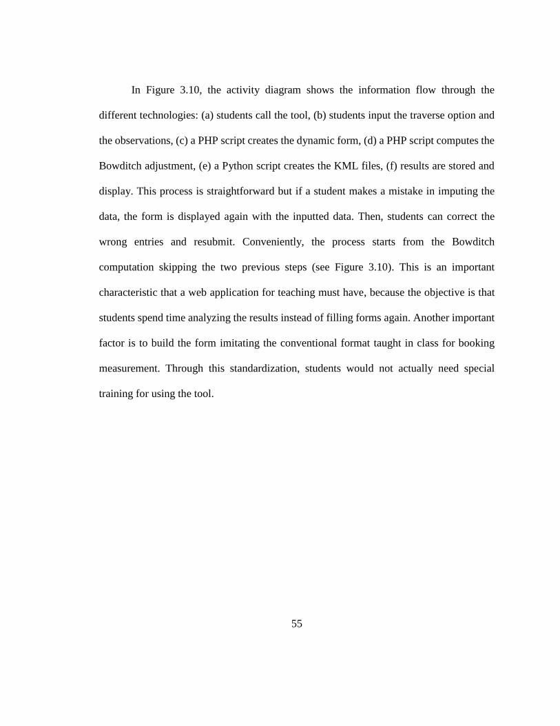
55
In Figure 3.10, the activity diagram shows the information flow through the
different technologies: (a) students call the tool, (b) students input the traverse option and
the observations, (c) a PHP script creates the dynamic form, (d) a PHP script computes the
Bowditch adjustment, (e) a Python script creates the KML files, (f) results are stored and
display. This process is straightforward but if a student makes a mistake in imputing the
data, the form is displayed again with the inputted data. Then, students can correct the
wrong entries and resubmit. Conveniently, the process starts from the Bowditch
computation skipping the two previous steps (see Figure 3.10). This is an important
characteristic that a web application for teaching must have, because the objective is that
students spend time analyzing the results instead of filling forms again. Another important
factor is to build the form imitating the conventional format taught in class for booking
measurement. Through this standardization, students would not actually need special
training for using the tool.
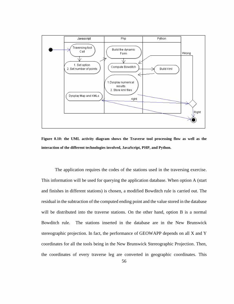
56
Figure 0.10: the UML activity diagram shows the Traverse tool processing flow as well as the
interaction of the different technologies involved, JavaScript, PHP, and Python.
The application requires the codes of the stations used in the traversing exercise.
This information will be used for querying the application database. When option A (start
and finishes in different stations) is chosen, a modified Bowditch rule is carried out. The
residual in the subtraction of the computed ending point and the value stored in the database
will be distributed into the traverse stations. On the other hand, option B is a normal
Bowditch rule. The stations inserted in the database are in the New Brunswick
stereographic projection. In fact, the performance of GEOWAPP depends on all X and Y
coordinates for all the tools being in the New Brunswick Stereographic Projection. Then,
the coordinates of every traverse leg are converted in geographic coordinates. This
57
transformation is computed using the formulae described by Thomson et al., (1977). The
parameters were used for this transformation are shown next:
X0 = 2500000 m coordinate X origin of the projection
Y0 = 7500000 m coordinate Y origin of the projection
R = 6379303.380 m radius of the conformal sphere evaluated in Theta (0)
K0 = 0.999912 scale factor
a = 6378137 m semi-major axis
b = 6356752.3141403561 m semi-minor axis
lat_0 = 46.5o latitude of the origin
lon_0 = -66.5o Longitude of the origin
This transformation function was tested with the Coordinate Transformation
Service (CTS) of Service New Brunswick (http://geonb.snb.ca/CTS/). Table 3.2 shows a
comparison of the results.
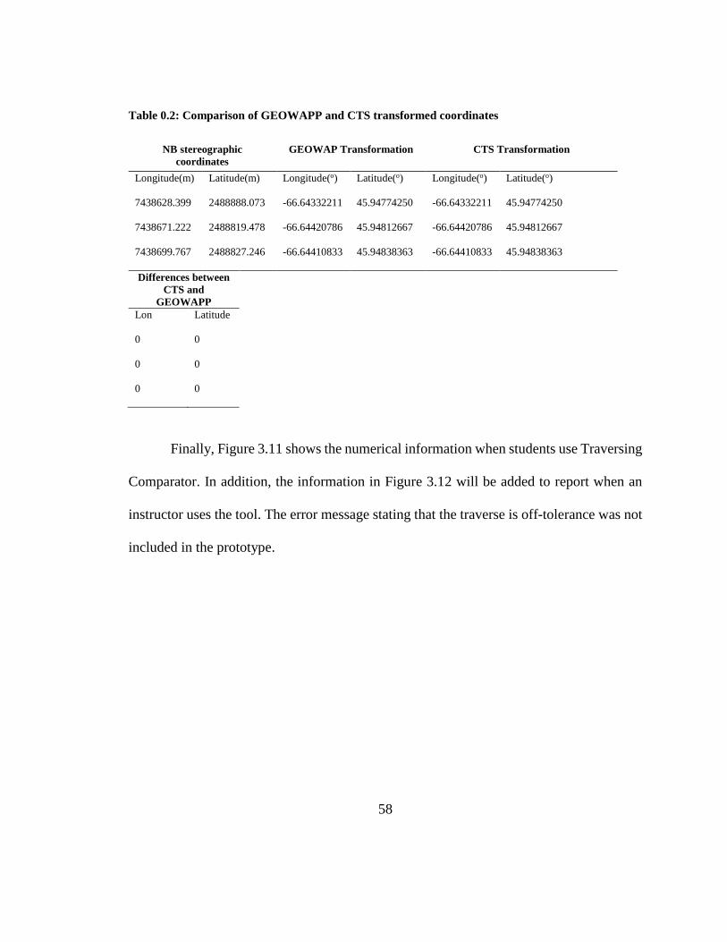
58
Table 0.2: Comparison of GEOWAPP and CTS transformed coordinates
NB stereographic
coordinates
GEOWAP Transformation CTS Transformation
Longitude(m) Latitude(m) Longitude(o) Latitude(o) Longitude(o) Latitude(o)
7438628.399 2488888.073 -66.64332211 45.94774250 -66.64332211 45.94774250
7438671.222 2488819.478 -66.64420786 45.94812667 -66.64420786 45.94812667
7438699.767 2488827.246 -66.64410833 45.94838363 -66.64410833 45.94838363
Differences between
CTS and
GEOWAPP
Lon Latitude
0 0
0 0
0 0
Finally, Figure 3.11 shows the numerical information when students use Traversing
Comparator. In addition, the information in Figure 3.12 will be added to report when an
instructor uses the tool. The error message stating that the traverse is off-tolerance was not
included in the prototype.

59
Figure 0.11: students will access this information when they are using the tool by themselves. The
residuals, linear misclosure and traverse length are in meters.
Figure 0.12: this information will be added to the information displayed in figure 3.11 when an
instructor is using Traversing Comparator. The latitudes, departures, distances and coordinates are
in meters.
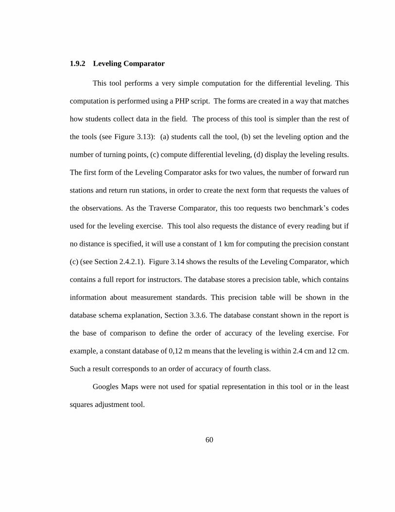
60
1.9.2 Leveling Comparator
This tool performs a very simple computation for the differential leveling. This
computation is performed using a PHP script. The forms are created in a way that matches
how students collect data in the field. The process of this tool is simpler than the rest of
the tools (see Figure 3.13): (a) students call the tool, (b) set the leveling option and the
number of turning points, (c) compute differential leveling, (d) display the leveling results.
The first form of the Leveling Comparator asks for two values, the number of forward run
stations and return run stations, in order to create the next form that requests the values of
the observations. As the Traverse Comparator, this too requests two benchmark’s codes
used for the leveling exercise. This tool also requests the distance of every reading but if
no distance is specified, it will use a constant of 1 km for computing the precision constant
(c) (see Section 2.4.2.1). Figure 3.14 shows the results of the Leveling Comparator, which
contains a full report for instructors. The database stores a precision table, which contains
information about measurement standards. This precision table will be shown in the
database schema explanation, Section 3.3.6. The database constant shown in the report is
the base of comparison to define the order of accuracy of the leveling exercise. For
example, a constant database of 0,12 m means that the leveling is within 2.4 cm and 12 cm.
Such a result corresponds to an order of accuracy of fourth class.
Googles Maps were not used for spatial representation in this tool or in the least
squares adjustment tool.

61
Figure 0.13: the UML activity diagram shows the Levelling tool processing flow as well as the
interaction of the different technologies involved, JavaScript, PHP, and Python.
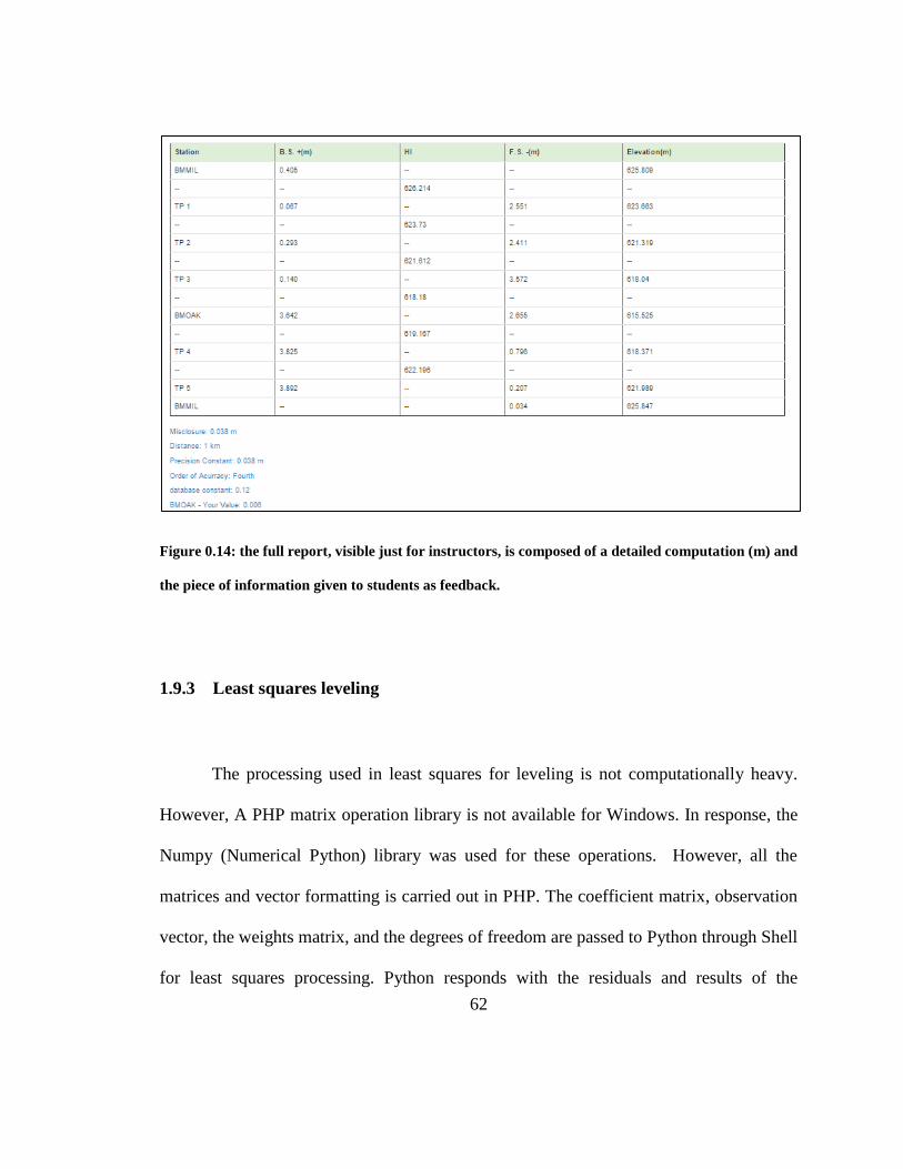
62
Figure 0.14: the full report, visible just for instructors, is composed of a detailed computation (m) and
the piece of information given to students as feedback.
1.9.3 Least squares leveling
The processing used in least squares for leveling is not computationally heavy.
However, A PHP matrix operation library is not available for Windows. In response, the
Numpy (Numerical Python) library was used for these operations. However, all the
matrices and vector formatting is carried out in PHP. The coefficient matrix, observation
vector, the weights matrix, and the degrees of freedom are passed to Python through Shell
for least squares processing. Python responds with the residuals and results of the
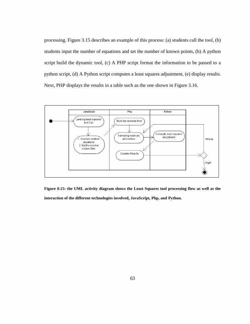
63
processing. Figure 3.15 describes an example of this process: (a) students call the tool, (b)
students input the number of equations and set the number of known points, (b) A python
script build the dynamic tool, (c) A PHP script format the information to be passed to a
python script, (d) A Python script computes a least squares adjustment, (e) display results.
Next, PHP displays the results in a table such as the one shown in Figure 3.16.
Figure 0.15: the UML activity diagram shows the Least Squares tool processing flow as well as the
interaction of the different technologies involved, JavaScript, Php, and Python.

64
Figure 0.16: the first table shows the full report composed by the results of the observation equation
(m), weights, and residuals (m). The second table provides the final elevation (m) of the unknown and
the standard deviations (m).
1.9.4 Proximity Comparator
The theory for this tool is discussed in Section 2.4.4.1. Here, common parameters
are assigned to compute the CEP, which is used to test the points’ proximity. For instance,
500m is the longest designed shot, which means that students commonly will not measure
longer distances. Next, a Topcon model GTS-105 will be chosen as the instrument that will
be used in the field practices, which has an EDM error (see Section 2.4.5) of 2 mm + 2ppm
(Topcon Corporation, 2006). This equipment is used in the first survey camps. Finally, the
survey accuracy will be 1: 5000; this accuracy sets the internal error using Table 2.6. An
example is given next (see Figure 3.17).

65
Allowed internal angular error (𝝈𝒊)
tan 𝜎𝑖 ≈ 𝜎𝑖 𝑟𝑎𝑑
𝜎𝑖= 1”.39 = 6.7389 x 10⁻⁶ rad
For 500 m, 𝜎𝑖 is transformed in distance using tan 𝜎𝑖= 𝜎𝑖 𝑖𝑛 𝑚𝑒𝑡𝑒𝑟𝑠 /500m ≈ 𝜎𝑖 𝑟𝑎𝑑
𝜎𝑖 𝑖𝑛 𝑚𝑒𝑡𝑒𝑟𝑠= 6.7389 x 10−6 ∗ 500 𝑚 ≈ 0.0034 𝑚
EDM Error (𝝈𝑬𝑫𝑴)
EDM = 0.0022 m + (2∗500
1 000 000)2 m = 0.0022 m
EDM Error + angular error
(√𝝈𝑬𝑫𝑴𝟐 + 𝝈𝒊 𝒊𝒏 𝒎𝒆𝒕𝒆𝒓𝒔
𝟐 )
√0.00222 + 0.00342 = 0.004 mm
Figure 0.17: as EDM error (𝛔𝐄𝐃𝐌) and internal angle error (𝛔𝐢 𝐢𝐧 𝐦𝐞𝐭𝐞𝐫𝐬) are independent error, they
should be added in square form and then square rooted to compute the magnitude of the error
combination.
SFE (4mm) should be added to the computation before for computing the total
tolerance. In this instance, SFE is chosen subjectively for reasons specified in Section
2.4.4.1. Table 3.3 shows the Feature Tolerance table, which shows the computation of the
total tolerance or CEP (Circular Error Probable) radius.
66
Table 0.3: computation of the total tolerance. In other words, computation of the CEP radius.
New feature coding system Feature type 𝛔𝐢 and EDMs
(m)
𝐒𝐅𝐄 (m) Total tolerance
(m)
BL Buildings 0.004 0.040 0.0402
BN Benches 0.004 0.100 0.1001
BR Bike racks 0.004 0.100 0.1001
Contours Contour lines 0.004 NA NA
CB Curbs 0.004 0.100 0.1001
EB Electrical boxes 0.004 0.040 0.0402
FN Fences 0.004 0.040 0.0402
GF Green fields 0.004 Na NA
HD Hydrants 0.004 0.100 0.1001
LI Lights 0.004 0.100 0.1001
LP Lamp posts 0.004 0.100 0.1001
MH Manholes 0.004 0.050 0.0502
PG Play grounds 0.004 0.100 0.1001
PL Parking areas 0.004 0.100 0.1001
SI Signs 0.004 0.100 0.1001
ST Streets 0.004 0.100 0.1001
SD Storm drains 0.004 0.100 0.1001
SW Sidewalks or any type of
walkways
0.004 0.100 0.1001
WA Treed or wooded areas 0.004 NA NA
TR Trees 0.004 0.100 0.1001
RW Retaining Walls 0.004 0.100 0.1001
TP Telephone poles 0.004 0.040 0.0402
In the application, a similar table will be stored in a MySQL database and the data
are retrieved to compare students’ observed features coordinates to the known feature
coordinates. This table schema is shown in Section 3.3.6. This table is an important element
for the performance of this tool because it is the basis of the comparison. Every known
topographic feature (KTF) coordinate is compared with the closest student observed
topographic feature (SOTF) coordinates with the same codification and tested to determine
if it meets the tolerance. The tool stores the KTF coordinates in a folder called
horizontal_samples, which is a comma-separated value (CSV) file. For the processing, this
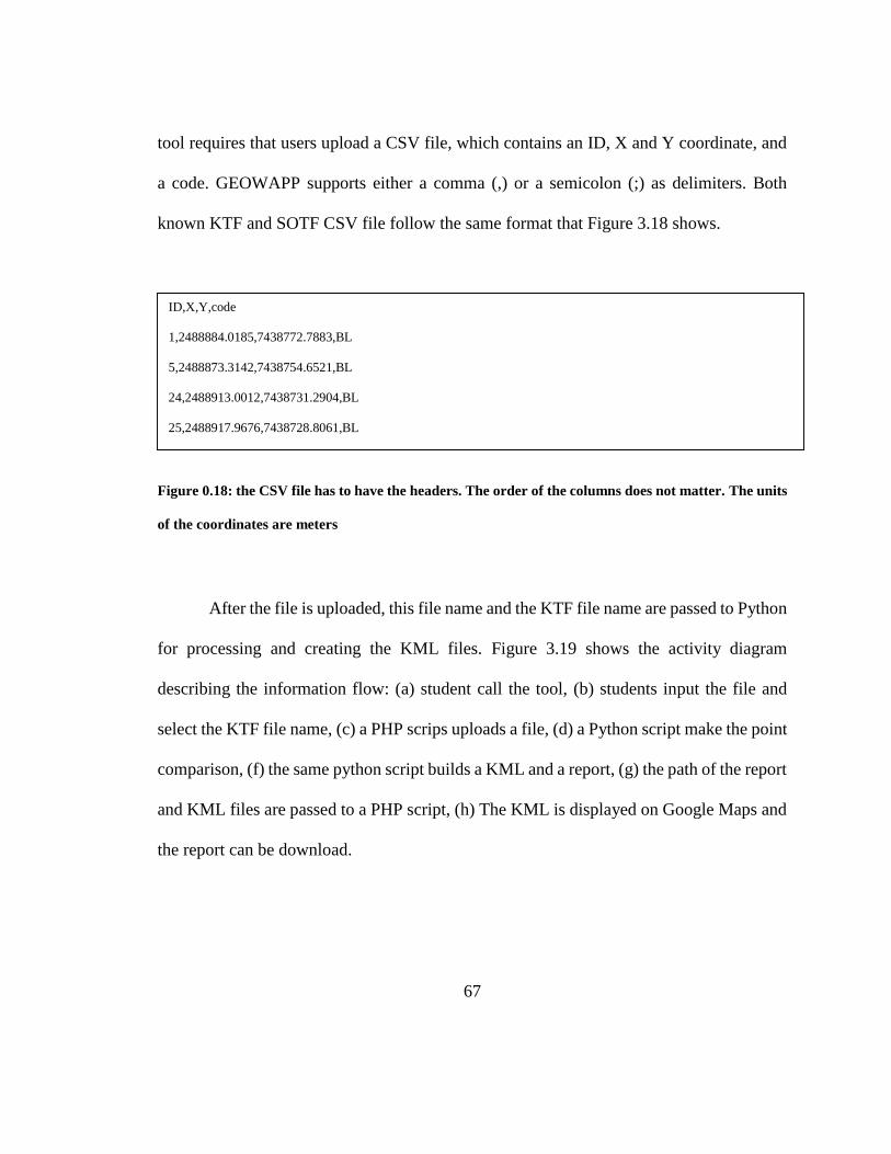
67
tool requires that users upload a CSV file, which contains an ID, X and Y coordinate, and
a code. GEOWAPP supports either a comma (,) or a semicolon (;) as delimiters. Both
known KTF and SOTF CSV file follow the same format that Figure 3.18 shows.
Figure 0.18: the CSV file has to have the headers. The order of the columns does not matter. The units
of the coordinates are meters
After the file is uploaded, this file name and the KTF file name are passed to Python
for processing and creating the KML files. Figure 3.19 shows the activity diagram
describing the information flow: (a) student call the tool, (b) students input the file and
select the KTF file name, (c) a PHP scrips uploads a file, (d) a Python script make the point
comparison, (f) the same python script builds a KML and a report, (g) the path of the report
and KML files are passed to a PHP script, (h) The KML is displayed on Google Maps and
the report can be download.
ID,X,Y,code
1,2488884.0185,7438772.7883,BL
5,2488873.3142,7438754.6521,BL
24,2488913.0012,7438731.2904,BL
25,2488917.9676,7438728.8061,BL
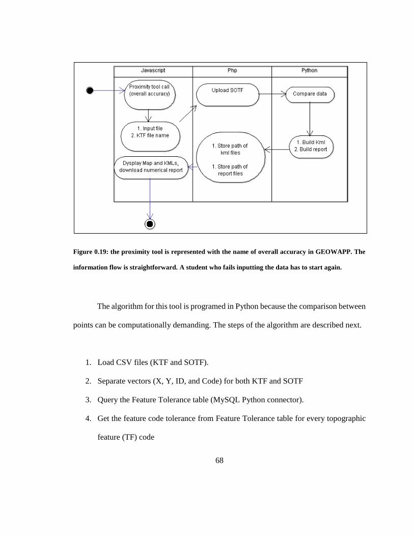
68
Figure 0.19: the proximity tool is represented with the name of overall accuracy in GEOWAPP. The
information flow is straightforward. A student who fails inputting the data has to start again.
The algorithm for this tool is programed in Python because the comparison between
points can be computationally demanding. The steps of the algorithm are described next.
1. Load CSV files (KTF and SOTF).
2. Separate vectors (X, Y, ID, and Code) for both KTF and SOTF
3. Query the Feature Tolerance table (MySQL Python connector).
4. Get the feature code tolerance from Feature Tolerance table for every topographic
feature (TF) code

69
5. For every TF code:
5.1 Create an empty list for the KTF index value.
5.2 Attach a KTF index value if it is equal to TF code
5.3 Repeat 5.1 and 5.2 for SOTF
5.4 For each KTF
5.4.1 Compute the distance to SOTF
5.4.2 For each SOTF
5.4.2.1 Find the shortest distance to KTF
5.4.2.2 Find SOTF feature index value.
5.4.3 Compare the shortest distance to the tolerance value and store red if off-
tolerance or green if in-tolerance.
5.4.4 Store the KTF index value
5.4.5 Store the shortest distance.
5.4.6 Store the closest index SOTF value
6. Compute the RMS with step five results
7. Transform from NB stereographic to NAD83
8. Create KMLs file and a numerical report.
Figure 3.20, for the graphical representation, and Figure 3.21, for the numerical
representation, show examples of the output. These outputs are computed with an
artificially generated topographic feature (TF) coordinates. The KML file shows the
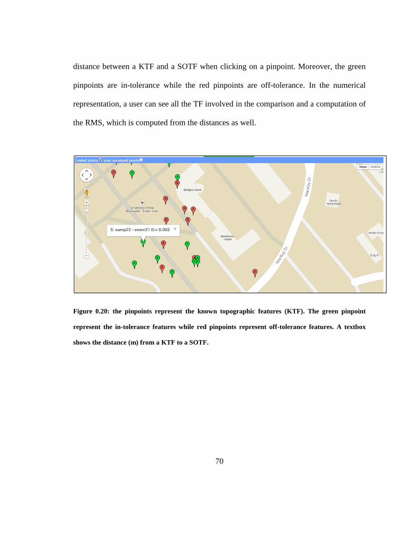
70
distance between a KTF and a SOTF when clicking on a pinpoint. Moreover, the green
pinpoints are in-tolerance while the red pinpoints are off-tolerance. In the numerical
representation, a user can see all the TF involved in the comparison and a computation of
the RMS, which is computed from the distances as well.
Figure 0.20: the pinpoints represent the known topographic features (KTF). The green pinpoint
represent the in-tolerance features while red pinpoints represent off-tolerance features. A textbox
shows the distance (m) from a KTF to a SOTF.
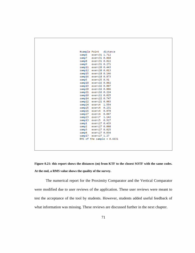
71
Figure 0.21: this report shows the distances (m) from KTF to the closest SOTF with the same codes.
At the end, a RMS value shows the quality of the survey.
The numerical report for the Proximity Comparator and the Vertical Comparator
were modified due to user reviews of the application. These user reviews were meant to
test the acceptance of the tool by students. However, students added useful feedback of
what information was missing. These reviews are discussed further in the next chapter.

72
1.9.5 Vertical Comparator
Section 2.4.4.2 describes a couple of options to create this tool, with a TIN/DEM
or with some known ground points (KGP) stored in the application as CSV. This last option
was implemented for the prototype because it is easier to program. The CSV files, for both
KGP and students’ observed ground points (SOGP), have to have at least the following
information: an ID, X and Y coordinate, and elevation (Z). Figure 3.22 shows an example
of the file format.
Figure 0.22: this CSV file have to have an Id, Y and X coordinate, and height (Z). In addition, the
delimiter can be a semicolon (;) or a comma (,). The units of the coordinates are meters.
The information flow is similar to of the Proximity Comparator tool. However, this
tool does not need to retrieve any table from the database. The users must provide some
information such as KGP file name, the accuracy that is needed, and the number of points
used for interpolating the z coordinate of KGP. This information along with the uploaded
file is passed to Python for processing, creating the KML files, and the numerical reports.
Figure 3.22 shows the form used for gathering this information. This information is passed
to Python through a shell command. Next, a Python script returns the names of the KML
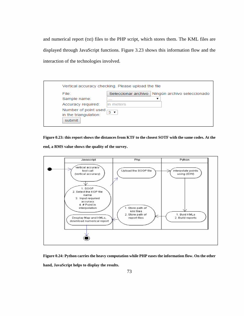
73
and numerical report (txt) files to the PHP script, which stores them. The KML files are
displayed through JavaScript functions. Figure 3.23 shows this information flow and the
interaction of the technologies involved.
Figure 0.23: this report shows the distances from KTF to the closest SOTF with the same codes. At the
end, a RMS value shows the quality of the survey.
Figure 0.24: Python carries the heavy computation while PHP eases the information flow. On the other
hand, JavaScript helps to display the results.
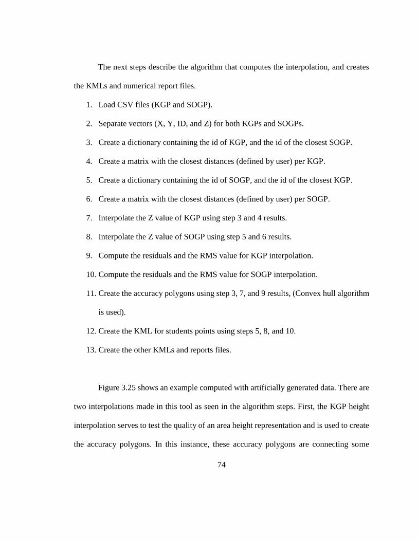
74
The next steps describe the algorithm that computes the interpolation, and creates
the KMLs and numerical report files.
1. Load CSV files (KGP and SOGP).
2. Separate vectors (X, Y, ID, and Z) for both KGPs and SOGPs.
3. Create a dictionary containing the id of KGP, and the id of the closest SOGP.
4. Create a matrix with the closest distances (defined by user) per KGP.
5. Create a dictionary containing the id of SOGP, and the id of the closest KGP.
6. Create a matrix with the closest distances (defined by user) per SOGP.
7. Interpolate the Z value of KGP using step 3 and 4 results.
8. Interpolate the Z value of SOGP using step 5 and 6 results.
9. Compute the residuals and the RMS value for KGP interpolation.
10. Compute the residuals and the RMS value for SOGP interpolation.
11. Create the accuracy polygons using step 3, 7, and 9 results, (Convex hull algorithm
is used).
12. Create the KML for students points using steps 5, 8, and 10.
13. Create the other KMLs and reports files.
Figure 3.25 shows an example computed with artificially generated data. There are
two interpolations made in this tool as seen in the algorithm steps. First, the KGP height
interpolation serves to test the quality of an area height representation and is used to create
the accuracy polygons. In this instance, these accuracy polygons are connecting some
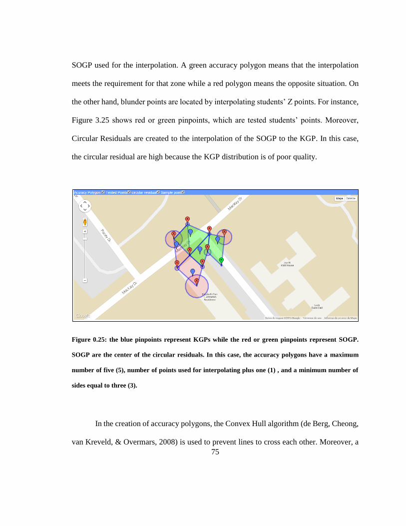
75
SOGP used for the interpolation. A green accuracy polygon means that the interpolation
meets the requirement for that zone while a red polygon means the opposite situation. On
the other hand, blunder points are located by interpolating students’ Z points. For instance,
Figure 3.25 shows red or green pinpoints, which are tested students’ points. Moreover,
Circular Residuals are created to the interpolation of the SOGP to the KGP. In this case,
the circular residual are high because the KGP distribution is of poor quality.
Figure 0.25: the blue pinpoints represent KGPs while the red or green pinpoints represent SOGP.
SOGP are the center of the circular residuals. In this case, the accuracy polygons have a maximum
number of five (5), number of points used for interpolating plus one (1) , and a minimum number of
sides equal to three (3).
In the creation of accuracy polygons, the Convex Hull algorithm (de Berg, Cheong,
van Kreveld, & Overmars, 2008) is used to prevent lines to cross each other. Moreover, a
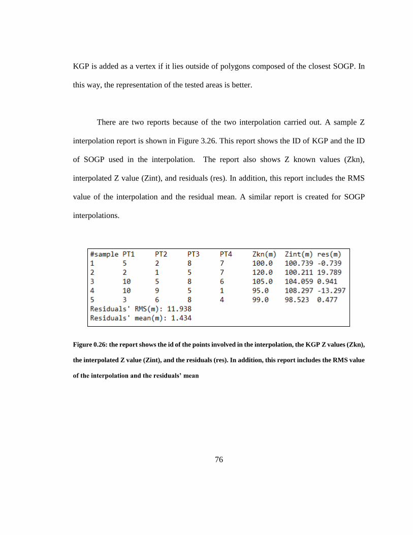
76
KGP is added as a vertex if it lies outside of polygons composed of the closest SOGP. In
this way, the representation of the tested areas is better.
There are two reports because of the two interpolation carried out. A sample Z
interpolation report is shown in Figure 3.26. This report shows the ID of KGP and the ID
of SOGP used in the interpolation. The report also shows Z known values (Zkn),
interpolated Z value (Zint), and residuals (res). In addition, this report includes the RMS
value of the interpolation and the residual mean. A similar report is created for SOGP
interpolations.
Figure 0.26: the report shows the id of the points involved in the interpolation, the KGP Z values (Zkn),
the interpolated Z value (Zint), and the residuals (res). In addition, this report includes the RMS value
of the interpolation and the residuals’ mean

77
1.10 Database Implementation
In Section 2.5, there are three (3) main groups defining the classification of the
database’s tables: sample or control points, Users, and Precision tables. As TXT files store
sample points (KTF, KGP ) in the application, these tables are not implemented in the data
base. The database structure is very simple because there is no relationship among the
tables. The five (5) tables created for this prototype are benchmark, feature tolerance,
leveling precision, stations, and users table. Figure 3.27 shows UML class diagram for
these tables used by GEOWAPP. The ID field for the tables is used as an alternative key
(<<AK>>), which auto incremental field. There is an ambiguity for the meaning of code.
For instance, code means the name of the station or benchmark in the benchmark
(bench_mark) or stations (Station) table, while in the Feature Tolerance table
(feature_tolerance) is the codification specified in Table 2.3. The precision fields in tables
Stations and Bench_marks are standard deviation values associated with the respective
coordinates. Finally, the c constant in leveling_precision_table is computed from Eq. 2.6
in Section 2.4.2.1.
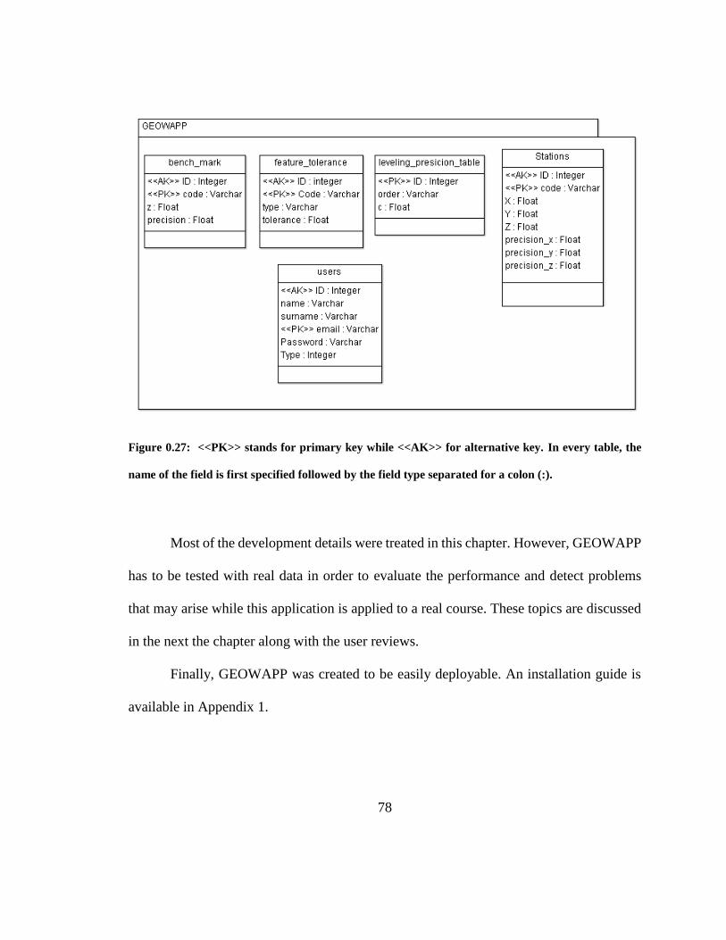
78
Figure 0.27: <<PK>> stands for primary key while <<AK>> for alternative key. In every table, the
name of the field is first specified followed by the field type separated for a colon (:).
Most of the development details were treated in this chapter. However, GEOWAPP
has to be tested with real data in order to evaluate the performance and detect problems
that may arise while this application is applied to a real course. These topics are discussed
in the next the chapter along with the user reviews.
Finally, GEOWAPP was created to be easily deployable. An installation guide is
available in Appendix 1.
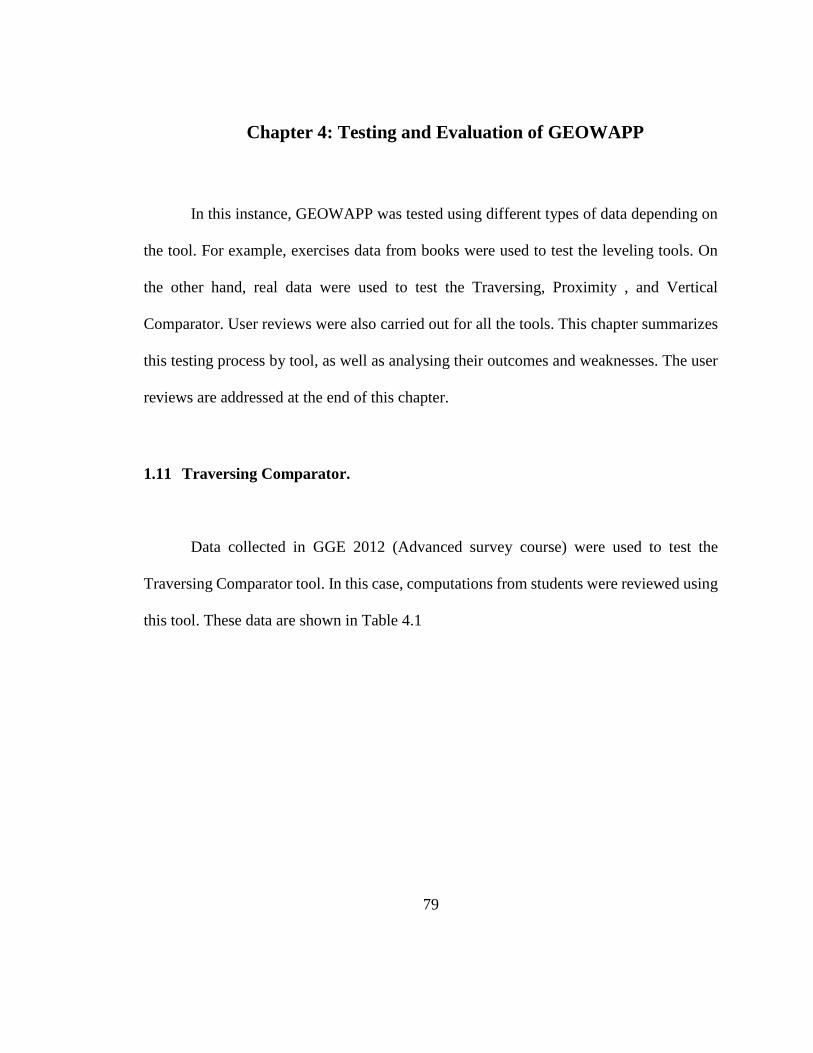
79
Chapter 4: Testing and Evaluation of GEOWAPP
In this instance, GEOWAPP was tested using different types of data depending on
the tool. For example, exercises data from books were used to test the leveling tools. On
the other hand, real data were used to test the Traversing, Proximity , and Vertical
Comparator. User reviews were also carried out for all the tools. This chapter summarizes
this testing process by tool, as well as analysing their outcomes and weaknesses. The user
reviews are addressed at the end of this chapter.
1.11 Traversing Comparator.
Data collected in GGE 2012 (Advanced survey course) were used to test the
Traversing Comparator tool. In this case, computations from students were reviewed using
this tool. These data are shown in Table 4.1

80
Table 0.1: students2015 data form GGE 2012.
Station Azimuth Dist. (m)
Degrees Minutes Seconds
1
270 29 22.2 14.720
2
253 21 14.4 17.244
3
166 12 58.6 30.853
4
78 04 12.8 24.391
5
00 00 00 29.742
1
There is little difference when comparing the GEOWAPP results to the students’
results. For example, the GEOWAPP results show the total traverse length of 116.950 m
while students’ results show 116.952 m, which is wrong. Likewise, the differences for the
latitude’s and departure’s misclosures are on the order of millimetres. All these differences
may be due to rounding errors and some small human errors by students since GEOWAPP
was tested using exercises from Wolf and Ghilani (2006).
In addition, a GGE 2012 group of students asked for help because they had a bug
in their computations. This situation presented a good opportunity to test GEOWAPP’s
value for supporting students. The instructor’s option was used to create a full report of the
computations, which helped these students to confirm that their calculation procedure was
right even though the results were still wrong. However, students found by themselves that
they flipped some decimals of a distance, which caused the wrong results. This event shows
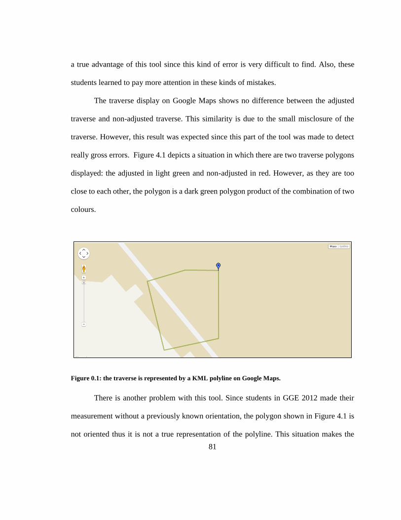
81
a true advantage of this tool since this kind of error is very difficult to find. Also, these
students learned to pay more attention in these kinds of mistakes.
The traverse display on Google Maps shows no difference between the adjusted
traverse and non-adjusted traverse. This similarity is due to the small misclosure of the
traverse. However, this result was expected since this part of the tool was made to detect
really gross errors. Figure 4.1 depicts a situation in which there are two traverse polygons
displayed: the adjusted in light green and non-adjusted in red. However, as they are too
close to each other, the polygon is a dark green polygon product of the combination of two
colours.
Figure 0.1: the traverse is represented by a KML polyline on Google Maps.
There is another problem with this tool. Since students in GGE 2012 made their
measurement without a previously known orientation, the polygon shown in Figure 4.1 is
not oriented thus it is not a true representation of the polyline. This situation makes the

82
contextual information from Google Maps less useful. Also, at least one of the traverse
points has to be a known coordinate in NB Stereographic double projection. Therefore,
some of the course curriculum should be changed in order to include such an application.
Moreover, the internal angle method for measuring a traverse is applied in GGE 2012,
which requires intermediate computations for acquiring the azimuth and may be
cumbersome for students. Thus, a tool should be made in order to test these computations
as well.
1.12 Leveling Comparator and Least Squares tool
These tools were tested with book exercises, from Wolf and Ghilani, 2006, and
Wolf and Ghilani, 1997. The Leveling comparator tool showed the same values as the
book exercise (Wolf & Ghilani, 2006. pp. 107). On the other hand, the Least Squares tool
was tested with two exercises (Wolf & Ghilani, 2006. pp. 107; Wolf & Ghilani, 1997. pp.
214). These two exercises are a non-weighted and a weighted exercise respectively. The
results of the GEOWAPP computation were the same showing the consistency of the tool.
In theory, the Leveling Comparator tool was developed to test the observation
against the computation of misclosures. Also, this tool was designed to test the students’
ability to read the rod by comparing students height computation to the height stored in the
database. Unfortunately, this assumption could not be tested with real data because this
tool was not applicable to GGE courses. On the other hand, the Least Square tool was
designed for advanced students. The idea was to provide a tool that could help them to test

83
their measurement in the field. However, senior students have already a good knowledge
about gathering measurements. Thus, this tool does not provide any learning value. In
contrast, the Leveling Comparator tool may have a teaching value since it is designed for
beginners.
1.13 Proximity Comparator tool
The proximity comparator tool was tested with real data, from advanced survey
camps of two years, 2014 and 2013. The 2013 data were chosen as KGP stored in the
database while 2014 data were chosen as SOGP. Furthermore, just some point
codifications were chosen: building (BL), manhole (MH), tree (TR), and lamppost (LP).
This decision is due to the non-standardization of the data codification, which makes it
difficult to match codes with features, because the 2014 data did not present any legend for
its codification. In order to do this test, the 2013 data are assumed to be very reliable and
accurate. From Table 2.3, the tolerance values are 0.042 for BL and 0.1001 for MH, TR,
and LP. Figure 4.2 shows the results of the dataset comparison.
84
Figure 0.2: the red pinpoints show that no point is within the tolerance. Moreover, the textbox shows
how far apart (in m) the KTF with code BL is from a point from the tested dataset.
As seen in figure 4.2, no point from the 2014 dataset is within the tolerance with
respect to the 2013 dataset. These results seem like a failure but it provides an insight: there
is a mismatch between the two datasets, which means that there is a mistake in the data
gathering. Moreover, there are 214 SOGPs being tested. Such a task is impossible to carry
out with a traditional reviewing method.
The comparison computation is not computationally demanding. In this instance, there
were 9061 comparisons carried out added to three (3) files created with a processing time
of 0.1 seconds. This processing time can be improved by adding a data management system
and indexes.
On the other hand, there are important details that should be taken into
consideration. For example, if a survey involved a determination of some station using

85
GPS, how to carry out the post-processing is of great importance since the first coordinates
might shift the results. However, statistical testing can be applied to find this shift and
correct the data, which is possible to implement in this tool.
1.14 Vertical Comparator tool
The same data from the horizontal comparator tool were also used to test this tool.
However, these data were formatted differently (see Figure 3.19). In this case, a sample of
the 213 KGPs was chosen arbitrarily from the 2013 sample. This KGPs file was composed
of ground points (GP) such as PL (Parking areas), WA (Treed or wooded areas) in order to
have points representing the ground and not artificial structures. On the other hand, the
2014 data, consisting of 1139 points, were chosen as SOGP and, it was submitted without
filtering. For processing these data, the following options were chosen: four (4) closest
points for interpolation, and 0.5 m for the required tolerance. In Figure 4.3, there are two
accuracy polygons labeled as one (1) and two (2). As seen, the accuracy polygon 1 is off-
tolerance. A KGP (blue pinpoint) lies outside of the polygon formed by the four pinpoints
used for interpolating the KGP point height. As mentioned in chapter 3, the algorithm adds
the KGP point as a vertex in order to represent the area better. On the other hand, the
accuracy polygon 2 is in-tolerance, and the KGP point is inside the polygon formed by the
four (4) closest points. The processing time was less than four (4) seconds. This time
includes the two (2) interpolation and the generation of six (6) files, 4 KMLs and 2 reports.
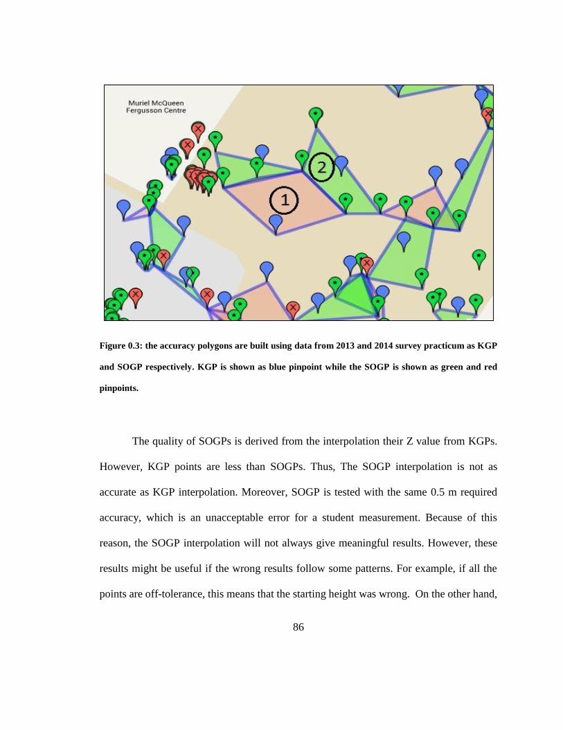
86
Figure 0.3: the accuracy polygons are built using data from 2013 and 2014 survey practicum as KGP
and SOGP respectively. KGP is shown as blue pinpoint while the SOGP is shown as green and red
pinpoints.
The quality of SOGPs is derived from the interpolation their Z value from KGPs.
However, KGP points are less than SOGPs. Thus, The SOGP interpolation is not as
accurate as KGP interpolation. Moreover, SOGP is tested with the same 0.5 m required
accuracy, which is an unacceptable error for a student measurement. Because of this
reason, the SOGP interpolation will not always give meaningful results. However, these
results might be useful if the wrong results follow some patterns. For example, if all the
points are off-tolerance, this means that the starting height was wrong. On the other hand,
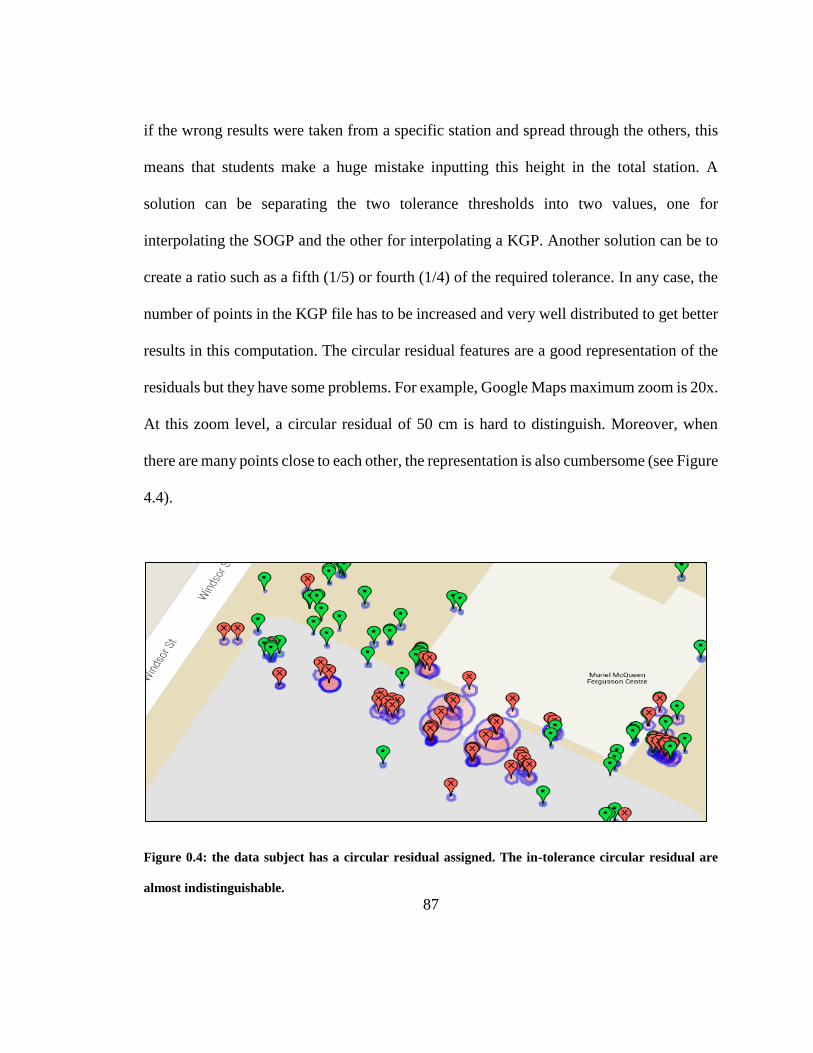
87
if the wrong results were taken from a specific station and spread through the others, this
means that students make a huge mistake inputting this height in the total station. A
solution can be separating the two tolerance thresholds into two values, one for
interpolating the SOGP and the other for interpolating a KGP. Another solution can be to
create a ratio such as a fifth (1/5) or fourth (1/4) of the required tolerance. In any case, the
number of points in the KGP file has to be increased and very well distributed to get better
results in this computation. The circular residual features are a good representation of the
residuals but they have some problems. For example, Google Maps maximum zoom is 20x.
At this zoom level, a circular residual of 50 cm is hard to distinguish. Moreover, when
there are many points close to each other, the representation is also cumbersome (see Figure
4.4).
Figure 0.4: the data subject has a circular residual assigned. The in-tolerance circular residual are
almost indistinguishable.

88
KGPs does not need to be a large number of points for measuring the quality of the
survey. For example, the RMS value was 0.347 m in this interpolation. This value shows
the students survey met the required accuracy. However, this measure has other issues in
the data representation. In the current way of representing the quality, a KGP sometimes
lie within a dense group of SOGPs. This situation produces a small accuracy polygon,
which sometimes is not very distinguishable and meaningful. Also, there are artificial
features involved in most of the surveys. These features have to be isolated for a correct
interpolation. Thus, the inclusion of breaklines is a necessary approach to make this tool
fully operational. On the other hand, different ways of representing the off-tolerance areas
should be explored such as a grid or circles surrounding the KGP.
In addition, the satellite view of Google Maps is a very useful tool where students
can see the distribution of their survey (see Figure 4.5). The parking lot in Figure 4.5 shows
the distribution of the students’ survey points using the satellite view. Also, the Google
Earth thin client has interesting functionality as well. For example, Figure 4.6 shows a
street view of with the accuracy polygon on top of it. The vertices of the accuracy polygons
are distinguishable using the KML option “relativeToGround”. This option can be
expanded to see SOGP position. However, this consideration is beyond the scope of this
research.

89
Figure 0.5: Accuracy polygons and the SOGP are shown in the surrounding area of a parking lot in
UNB.
Figure 0.6 : Accuracy polygons are shown on the Google Earth street view option
90
In summary, this tool can be very useful for students and instructors to review the
data collection process. Nevertheless, there have to be improvements in the way of
displaying which areas are well represented by student survey.
1.15 User Reviews
The user review survey (see Appendix 2) was designed to address three (3) basic
aspects: the numerical information provided, the dynamic maps generated, and the
application concept. The questions were designed to measure the acceptability of the tool
to students. In addition, two open questions were added in order to gather students ideas.
This decision turned out to be useful because there were modifications to the tool based on
student opinions.
The reviewers were students from the department of Geodesy and Geomatics and
other departments at UNB that have to take surveying courses in their curriculum. These
students are from all years but the first year. This decision was made because reviewers
had to have some experience with field practices in order to give useful feedback. These
17 students were asked to submit some data in one of the tools and answered the survey.
As seen in Appendix 2, students were given a number of options. To analyze
students’ answers, the option number was divided by the total of options and multiplied by
a hundred; The option number was ordered from the worst as one (1) to the best as three
or four (3 or 4). This computation will give a value within the range of 25 to 100 for every
question in the survey. For charts representation, a mean was computed from the values
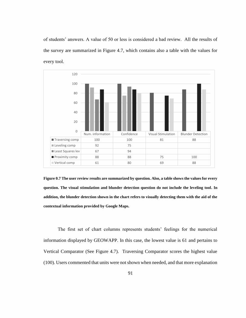
91
of students’ answers. A value of 50 or less is considered a bad review. All the results of
the survey are summarized in Figure 4.7, which contains also a table with the values for
every tool.
Figure 0.7 The user review results are summarized by question. Also, a table shows the values for every
question. The visual stimulation and blunder detection question do not include the leveling tool. In
addition, the blunder detection shown in the chart refers to visually detecting them with the aid of the
contextual information provided by Google Maps.
The first set of chart columns represents students’ feelings for the numerical
information displayed by GEOWAPP. In this case, the lowest value is 61 and pertains to
Vertical Comparator (See Figure 4.7). Traversing Comparator scores the highest value
(100). Users commented that units were not shown when needed, and that more explanation
Num. information Confidence Visual Stimulation Blunder Detection
Traversing comp 100 100 81 88
Leveling comp 92 75
Least Squares lev 67 94
Proximity comp 88 88 75 100
Vertical comp 61 80 69 88
0
20
40
60
80
100
120

92
should be provided for interpreting the results of this tool. The second set of columns shows
the confidence feeling for having this information while making measurement in the field.
In this instance, students’ feelings were favorable; the lowest value obtained was 80. In the
visual stimulation part, students were asked if the tools would help them to visualize their
work more effectively. This question was oriented towards the tools that show results on
Google Maps. Thus, the leveling tool was excluded of this measure as seen in Figure 4.7.
In this case, the lowest value is 70, which implies that students think that this would help
to visualize their work. The last set of columns from Figure 4.7 shows that students also
feel that the results displayed on Google Maps will help them to detect blunders. This
statement is made based on the lowest value of 88, which is a high value.
In the survey, a question was included to measure students’ feeling about a web
application for enhancing survey labs. In this instance, the entire set of tools can be
analyzed together because the question is highly generalized. Moreover, the choices in the
survey were meant to measure if students can be engaged by such an application. In this
case, students showed high interest in this application. Figure 4.8 compares the values
obtained by each tool with the overall value, which is 85.

93
Figure 0.8: students’ feelings about the concept is shown in this chart. The dark column shows the
evaluation of every tool while the lighter one shows the mean value that includes every tool.
High acceptance of this tool by students can be concluded based on the user
reviews. However, this result does not mean that the application is fully operational or that
this will increase the learning of students. These topics should be investigated in future
research.
0
10
20
30
40
50
60
70
80
90
100
Traversingcomp
Levelingcomp
Least Squareslev
Proximitycomp
Vertical comp
Feeling about the concept
Overal Value

94
Chapter 5: Discussion on the outcomes.
At the beginning, the hypothesis discusses enhancing teaching in survey lab
practices by utilizing a web tool. In order to prove or disprove this statement, the
GEOWAPP should be applied to a surveying engineering course in real life. This test was
not carried out in this research because the application was not ready to fully support the
survey practices. On the other hand, there was a hint of GEOWAPP’s enhancing
characteristic discussed in Section 4.1 where students received beneficial feedback in a
traverse practice. Moreover, Davis (2009) mentioned that mobile technology helps to
create dynamic and interactive environments inside and outside the classrooms. Motivating
students is also a challenge for instructors. Davis (2009) also advises the use of strategies
to engage students to learn. Since students show great interest in the GEOWAPP concept
(see Figure 4.8), this application can be a way to motivate students. Also, GEOWAPP is
designed to give feedback to students. This characteristic is of great importance since, in
fact, feedback is a very important component of the teaching process. This reasoning
supports the belief that such an application can enhance learning and be beneficial for
students.
The designing process took into account the interaction of the instructors and
students with GEOWAPP. This design is still valid since instructors should be able to
author the exercises. However, instructors have to have some knowledge about the
application and MySQL to post exercises in the current state of development of
GEOWAPP. Also, the interaction of the GEOWAPP components was modeled (see Figure

95
2.2). In this instance, the document catalog was not developed for the prototype. However,
this component is easy to program since it is just a repository of exercise examples. On the
other hand, a repository of exercise examples might be unnecessary because the
Desire2learn management system serves this purpose already.
The exercise schemata were designed based on an analysis of GGE 1001
(Introduction to Geodesy and Geomatics), GGE 1803 (Practicum for Civil Engineers), and
GGE 2013 (Advanced Survey Practicum). This analysis suggests that the best way to
enhanced survey practicums is being able to test accuracies of students’ deliverables in
different ways. By self-testing, students will gain confidence in their work if the results are
correct. In the other case, students can locate where mistakes are made in observations or
computations. Thus, accuracy was the pillar for designing and developing GEOWAPP.
However, exploring other options can be beneficial for students as well. For example,
applications that help step-by-step students to make computations or help to model
different situations (e.g. traverse, leveling exercises) can be an interesting approach.
Five (5) out of six (6) tools were designed because the network comparator is
beyond the scope of the purpose of the prototype. However, this tool can be can be worth
to consider in future developments. For this reason, the design of this tool remains in this
document. The application design has more information that what was developed in the
prototype to serve for future guidance. For example, the use of DEM is mentioned as an
alternative to testing students’ datasets. An important aspect that must be considered for

96
future developments is the creation of forms that simulate the standard booking techniques.
This consideration will reduce the amount of training for using the tools. A prototype was
developed using mainly PHP, Javascript, and Python. This decision is not restrictive
because there are many other combination of scripting languages. However, the processing
time for the most time consuming task was less than 4 seconds. This result is efficient
considering that a data management system was not used in its full capacity of interaction.
Thus, the chosen combination of technologies is still a valid option. The Google Maps API
was chosen in order to display the results. However, the OpenLayes API is also a valuable
option to explore.
A course curriculum should change in order to include a web application such as
GEOWAPP. These changes were described in Chapter 4. Also, accurate data must be
collected in the place where students usually have their practices. This task can be time
consuming but it can also be a one-time task if the monuments of the control points are
well maintained and thus their coordinates can be actualized every year. In fact, accurate
data are the basis that supports GEOWAPP and any similar application. An example is
shown in Section 4.3 where no point was found within tolerance. Maintaining these data
would not be a problem because data surveyed by students in the practicum can be used to
do so. On the other hand, the SFE (specific feature error) must be determined for
unexperienced observers in order to set realistic tolerances for every TF.
97
New ways of representing the tested areas must be explored since accuracy
polygons do not always give the best representation. Circles surrounding the KGP or a grid
representation stand as options to be developed.
The Least Squares Levelling Checking tool was considered inapplicable because
this tool was designed to give support to advanced students, which have already a good
knowledge of data collection. Thus, this tool does not provide a high teaching value. The
Leveling Comparator theoretically seems promising. Nevertheless, this might be not the
case since the computation of differential leveling is too easy. On the other hand, a dynamic
graphical representation of the computation could help students to visualize leveling
exercises.
The Traversing Comparator tool can help students to visualize their field work. This
tool showed the most promise because it was used to support a real exercise. On the other
hand, it can also be extensible to reduce internal angle measurement to azimuths where
students often have miscomputations. In the same way, the design of the toolbox allows
to add more tools to the application whenever it is considered proper. Then, the application
can be easily extended to support more exercises.
From the user reviews, students showed positive feelings for such an application
and its capabilities. This tendency does not necessarily mean that students believe that
GEOWAPP is ready to be applied in a course. However, students embrace the idea of an
application supporting surveying field practices.

98
Chapter 6: Conclusions.
This study explored the idea of creating a web application that can actively support
students in surveying field practices. This exploration comprises a process of designing,
creating, and testing this application compliant with the research objectives (RO1 to RO6)
(Section 1.3.3). In the designing process, (RO1) the interaction of the different users
(students and instructors) was modeled resulting a model of the application components.
(RO2) GGE 1001, GGE 1803, GGE 2013 course outlines were reviewed resulting in
exercises that could be supported by GEOWAPP. (RO3) The accuracy concept was chosen
as the GEOWAPP pillar, which leads to design how field practices can be supported, which
was discussed in Chapter 2. (RO4) The next step was to create a GEOWAPP prototype in
order to explore if this application produced meaningful results using real data. Based on
the model of application components, the technologies PHP, JavaScript, MySQL, and
Python were chosen for the GEOWAPP development. On the other hand, different
combination of technologies are not discarded for the development of such an application.
The Google Maps API was chosen in order to display the results. However, the OpenLayes
API could be also a valuable option to explore. There were six (6) tools designed and five
(5) developed (See Chapter 5): Traversing Comparator, Leveling Comparator, Least
Squares Checking, Proximity comparator, and Vertical Comparator. How to interpret the
application results has been discussed in Chapter 4. (RO5) The application functionality
was tested with real data and with textbook exercises. The functionality provides the

99
expected result from the design process. However, Least Squares Checking was not found
to be applicable, and the value of Leveling Comparator remains untested. Traversing
Comparator appeared to be the most promising tool because a teaching value was found.
When testing Proximity Comparator with real data, no point was found within the
tolerance. This result showed that the data that are used as known topographic feature
(KTF) have to be highly accurate and reliable. The Vertical Comparator showed a great
potential locating areas that are not well represented by student observed ground points
(SOGP). However, Accuracy Polygons appeared to have some deficiencies such as area
representation. Also, the density and distribution of the KGP has to be appropriate in order
to provide meaningful results. (RO6) Users reviews showed the positive feelings that
students have for such an application and its concept. However, this application is not ready
to be applied to a real course until some small changes are made to the course curriculum.
For instance, giving real starting coordinates and a backsight are necessary for most of the
tools. Also, accurate data from the survey location has to be gathered for accurate
comparisons. The hypothesis stated was not proved to the fullest extent because this must
be tested with a surveying course. However, the application is compliant with techniques
for enhancing teaching, and the traversing tool was used to solve a real life problem. Thus,
this application has teaching value. In addition, the design of GEOWAPP allows adding
more tools to the toolbox, which makes the application extensible. This consideration was
a part of the hypothesis, which was achieved. In future work, some features remain to be
developed such as a tool that includes internal angles reductions. Different representations

100
of tested areas for Vertical Comparator remain to be evaluated such as a grid or circles
surrounding the KGP. Also, the inclusion of breaklines in the solution should be developed
for this tool. Other improvement recommendations can be found in Chapter 4. The SFE
remain to be determined for inexperienced observers. Generally, this application must be
tested with a real life course assessing the students that use the GEOWAPP and students
that do not in order to prove if this application is advantageous for students. Finally, other
application focus could be useful. For example, an application that focuses on teaching
how to make either computation or observation step-by-step would have a worthy value.
(Kavanagh, 2009)
(Davis, 2009)
(Wolf & Ghilani, 2006)
(Thomson, Krakiwsky, & Steeves, 1977)
(Nickerson, 1978)

101
References
Aguilar, F., Aguilar, M., & Aguera, F. (2007). Accuracy assessment of digital elevation
models using a non-parametric approach. International Journal of Geographical
Information Science, 21(6)
Blak, T. (2007). DEM quality assessment. In D. Maune (Ed.), Digital elevation model
technologies and applications : The DEM users manual (2nd ed., pp. 430-431).
Bethesda, Md.: American Society for Photogrammetry and Remote Sensing.
Booch, G., Rumbaugh, J., & Jacobson, I. (1999). The unified modeling language user
guide. Reading, Mass.: Addison-Wesley.
Commission 2- Professional Education, FIG. (2010). Enhancing surveying education
through e-learning. The International Federation of Surveyors (FIG),
Dare, P. (2013a). Lab 1: Differential leveling [lab instructions]. Fredericton: University of
New Brunswick.
Dare, P. (2013b). Lab 2: Traverse assignment [lab instructions]. Fredericton: University
of New Brunswick.
Dare, P. (2013c). Lab 3: Topographic survey [lab instructions]. Fredericton: University of
New Brunswick.

102
Dare, P., & Akay, G. (2014). Advanced surveying practicum [course outline]. Fredericton:
University of New Brunswick.
Davis, B. G. (2009). Tools for teaching (2nd ed.). USA: Jossey-Bass Publishers.
de Berg, M., Cheong, O., van Kreveld, M., & Overmars, M. (2008). Covex hulls.
Computational geometry: Algorithms and applications (3th ed., pp. 243). Berlin:
Springer.
El-Mowafy, A., Kuhn, M., & Snow, T. (2013). A blended learning approach in higher
education: A case study from surveying education.
Gil, A., Núñez-Casillas, L., Isenburg, M., Benito, A., Bello, J., & Arbelo, M. (2013). A
comparison between LiDAR and photogrammetry digital terrain models in a forest
area on tenerife island. Canadian Journal of Remote Sensing, 39(5), 396-409.
Habib, E., Ma, Y., Williams, D., Sharif, H., & Hossain, F. (2012). HydroViz: Design and
evaluation of a web-based tool for improving hydrology education. Hydrology &
Earth System Sciences, 16(10)
Harasim, L. (2006). A history of e-learning: Shift happened. The international handbook
of virtual learning environments (pp. 59-94) Springer.

103
Harris, T. M., Rouse, L. J., & Bergeron, S. J. (2010). The geospatial web and local
geographical education. International Research in Geographical and Environmental
Education, 19(1), 63-66.
Hohle, J., & Hohle, M. (2009). Accuracy assessment of digital elevation models by means
of robust statistical methods. ISPRS Journal of Photogrammetry and Remote Sensing,
64(4), 398-406.
Kavanagh, B. F. (2009). Surveying : Principles and applications. Upper Saddle River, NJ:
Pearson/Prentice Hall.
Mathematical Analysis and Research Corp. (1987). Calculating the CEP. (FINAL No. D-
4770). CA, USA: Jet Propulsion Laboratory (JPL).
Means, B., Toyama, Y., Murphy, R., Bakia, M., & Jones, K. (2010). Evaluation of
evidence-based practices in online learning: A meta-analysis and review of online
learning studies. US Department of Education.
Milne, P. (1984). BASIC programs for land surveying. London; New York: E. & F.N.
Spon.
Nicholson, P. (2007). A history of e-learning. Computers and education (pp. 1-11)
Springer.

104
Nickerson, B. (1978). A priori estimation of variance for surveying observables. New
Brunswick: Dpt. Geodesy and Geomatics Engineering, University of New Brunswick.
Reutebuch, S., Ahmed, K., Curtis, T., Petermann, D., Wellander, M., & Froslie, M. (2000).
A test of airborne laser mapping under varying forest canopy. Paper presented at the
Proceedings of the ASPRS 2000 Annual Conference, 22-26.
Roberts, G., & Gray, J. (2010). Nest- A new web based teaching tool for engineering
surveying. FIG Congress 2010, Sydney, Australia.
Sepehr, S. (2009). Development of a geospatial reference Framework A case study for the
UNB-GGE survey camp. (Unpublished M. Sc.). University of New Brunswick,
Fredericton.
Soon, L. (2011). E-learning and m-learning: Challenges and barriers in distance education
group assignment collaboration. International Journal of Mobile and Blended
Learning (IJMBL), 3(3), 43-58.
Thomson, D., Krakiwsky, E., & Steeves, R. (1977). A manual for geodetic coodinate
transformation in the maritime provinces. ( No. TR48). Fredericton, NB, Canada.:
Department of Geodesy and Geomatics,University of New Brunswick.
Topcon Corporation. (2006). Instruction manual electronic total station, GTS-100N series.
Tokyo, Japan.: Topcon Corporation.

105
White, R., & Fraser, D. (2013). Practicum for civil engineers [course outline]. Fredericton:
University of New Brunswick.
Wolf, P., & Ghilani, C. (1997). Adjustment computations : Statistics and least squares in
surveying and GIS (3rd ed.). New York: John Wiley & Sons.
Wolf, P., & Ghilani, C. (2006). Elementary surveying: An introduction to geomatics (11th
ed.). USA: Pearson Prentice Hall.
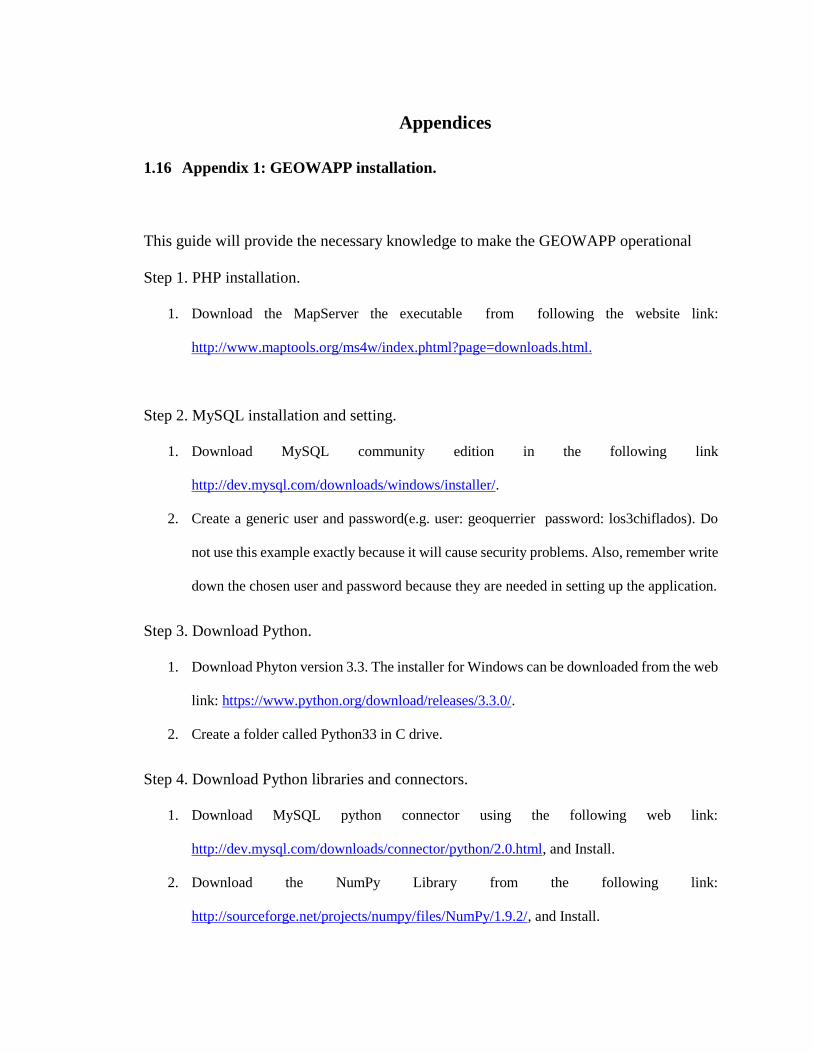
Appendices
1.16 Appendix 1: GEOWAPP installation.
This guide will provide the necessary knowledge to make the GEOWAPP operational
Step 1. PHP installation.
1. Download the MapServer the executable from following the website link:
http://www.maptools.org/ms4w/index.phtml?page=downloads.html.
Step 2. MySQL installation and setting.
1. Download MySQL community edition in the following link
http://dev.mysql.com/downloads/windows/installer/.
2. Create a generic user and password(e.g. user: geoquerrier password: los3chiflados). Do
not use this example exactly because it will cause security problems. Also, remember write
down the chosen user and password because they are needed in setting up the application.
Step 3. Download Python.
1. Download Phyton version 3.3. The installer for Windows can be downloaded from the web
link: https://www.python.org/download/releases/3.3.0/.
2. Create a folder called Python33 in C drive.
Step 4. Download Python libraries and connectors.
1. Download MySQL python connector using the following web link:
http://dev.mysql.com/downloads/connector/python/2.0.html, and Install.
2. Download the NumPy Library from the following link:
http://sourceforge.net/projects/numpy/files/NumPy/1.9.2/, and Install.

Step 5. Copy and paste the GEOWAPP in the htdocs folder.
1. For downloading the software, send an email to [email protected] to request the
software.
2. Unzip the folder and paste its contents in the following directory: C:/ms4w/Apache/htdocs/
Step 6. Create the database and the tables.
1. Create a file name geowap.sql using notepad and copy and paste the following commands:
CREATE DATABASE IF NOT EXISTS `geowapp` /*!40100 DEFAULT CHARACTER SET utf8 */; USE `geowapp`; -- MySQL dump 10.13 Distrib 5.6.17, for Win32 (x86) -- -- Host: atlas.gge.unb.ca Database: geowapp -- ------------------------------------------------------ -- Server version 5.6.21-log /*!40101 SET @OLD_CHARACTER_SET_CLIENT=@@CHARACTER_SET_CLIENT */; /*!40101 SET @OLD_CHARACTER_SET_RESULTS=@@CHARACTER_SET_RESULTS */; /*!40101 SET @OLD_COLLATION_CONNECTION=@@COLLATION_CONNECTION */; /*!40101 SET NAMES utf8 */; /*!40103 SET @OLD_TIME_ZONE=@@TIME_ZONE */; /*!40103 SET TIME_ZONE='+00:00' */; /*!40014 SET @OLD_UNIQUE_CHECKS=@@UNIQUE_CHECKS, UNIQUE_CHECKS=0 */; /*!40014 SET @OLD_FOREIGN_KEY_CHECKS=@@FOREIGN_KEY_CHECKS, FOREIGN_KEY_CHECKS=0 */; /*!40101 SET @OLD_SQL_MODE=@@SQL_MODE, SQL_MODE='NO_AUTO_VALUE_ON_ZERO' */; /*!40111 SET @OLD_SQL_NOTES=@@SQL_NOTES, SQL_NOTES=0 */; -- -- Table structure for table `bench_mark` -- DROP TABLE IF EXISTS `bench_mark`; /*!40101 SET @saved_cs_client = @@character_set_client */; /*!40101 SET character_set_client = utf8 */; CREATE TABLE `bench_mark` ( `ID` int(11) NOT NULL, `code` varchar(5) NOT NULL, `z` float NOT NULL, `precision` float NOT NULL ) ENGINE=InnoDB DEFAULT CHARSET=utf8; /*!40101 SET character_set_client = @saved_cs_client */; -- -- Table structure for table `feature_tolerance` -- DROP TABLE IF EXISTS `feature_tolerance`; /*!40101 SET @saved_cs_client = @@character_set_client */; /*!40101 SET character_set_client = utf8 */; CREATE TABLE `feature_tolerance` ( `id` int(11) NOT NULL,

`code` varchar(10) NOT NULL, `type` varchar(20) NOT NULL, `tolerance` float NOT NULL ) ENGINE=InnoDB DEFAULT CHARSET=utf8; /*!40101 SET character_set_client = @saved_cs_client */; -- -- Table structure for table `leveling_precision_table` -- DROP TABLE IF EXISTS `leveling_precision_table`; /*!40101 SET @saved_cs_client = @@character_set_client */; /*!40101 SET character_set_client = utf8 */; CREATE TABLE `leveling_precision_table` ( `ID` int(11) NOT NULL, `order` varchar(30) NOT NULL, `c` float NOT NULL ) ENGINE=InnoDB DEFAULT CHARSET=utf8; /*!40101 SET character_set_client = @saved_cs_client */; -- -- Table structure for table `stations` -- DROP TABLE IF EXISTS `stations`; /*!40101 SET @saved_cs_client = @@character_set_client */; /*!40101 SET character_set_client = utf8 */; CREATE TABLE `stations` ( `ID` int(11) NOT NULL AUTO_INCREMENT, `code` varchar(5) NOT NULL, `x` double NOT NULL, `y` double NOT NULL, `z` double NOT NULL, `precision_x` float NOT NULL, `precision_y` float NOT NULL, `precision_z` float NOT NULL, PRIMARY KEY (`ID`,`code`) ) ENGINE=InnoDB AUTO_INCREMENT=4 DEFAULT CHARSET=utf8; /*!40101 SET character_set_client = @saved_cs_client */; -- -- Table structure for table `users` -- DROP TABLE IF EXISTS `users`; /*!40101 SET @saved_cs_client = @@character_set_client */; /*!40101 SET character_set_client = utf8 */; CREATE TABLE `users` ( `ID` int(11) NOT NULL AUTO_INCREMENT, `name` varchar(20) NOT NULL, `surname` varchar(20) NOT NULL, `email` varchar(30) NOT NULL, `password` varchar(20) NOT NULL, `admin` int(1) NOT NULL, PRIMARY KEY (`ID`), UNIQUE KEY `ID` (`ID`), UNIQUE KEY `email` (`email`) ) ENGINE=InnoDB AUTO_INCREMENT=11 DEFAULT CHARSET=utf8; /*!40101 SET character_set_client = @saved_cs_client */; /*!40103 SET TIME_ZONE=@OLD_TIME_ZONE */;

/*!40101 SET SQL_MODE=@OLD_SQL_MODE */; /*!40014 SET FOREIGN_KEY_CHECKS=@OLD_FOREIGN_KEY_CHECKS */; /*!40014 SET UNIQUE_CHECKS=@OLD_UNIQUE_CHECKS */; /*!40101 SET CHARACTER_SET_CLIENT=@OLD_CHARACTER_SET_CLIENT */; /*!40101 SET CHARACTER_SET_RESULTS=@OLD_CHARACTER_SET_RESULTS */; /*!40101 SET COLLATION_CONNECTION=@OLD_COLLATION_CONNECTION */; /*!40111 SET SQL_NOTES=@OLD_SQL_NOTES */; -- Dump completed on 2015-05-24 15:47:47
2. Load geowap.sql using a MySQL interface program like phpMyAdmin or
MySQLworkbench.
3. Feed the required data using MySql functions.

Step 7. Changing the user and password for MySQL
1. Read the following information for MySQL-PHP connector function.
$connect=mysqli_connect("YourServerName.com:YourPort","YourUser",
"YourPassword","geowapp");
2. Change the following information in the PHP folder: “YourSeverName.com” by the server
URL will be used, “YourPort” by MySQL default port, and “YourUser” and
“YourPassword” by the user and password specified in Step 2. This information should be
change in the files listed below.
bowditch.php
compare_leveling_work.php
logged_in.php
leveling_least_squares.php
register.php
Read the following information for MySQL-Python connector function.
cnx = mysql.connector.connect(user='YourUser', password='YourPassword', host='YourSeverName.com',
database='geowapp')
Change the information in the following Python files in the Python folder
horizontal_accuracy.py
traverse_to_KML.py
Step 8 configuring the path for the KML files..
1. Set your KML folder address like the next example:
$kmlpath1 = 'http://atlas.gge.unb.ca/geowapp/KMLS/'.$KML_name_1;
And, so on with similar variables.
2. Change the text marked in the following files.
bowditch.php

vertical_accuracy.php
horizontal_accuracy.php
Step 9. Access the web application using http://YourServerName.com/geowap/index.php
and play with it.
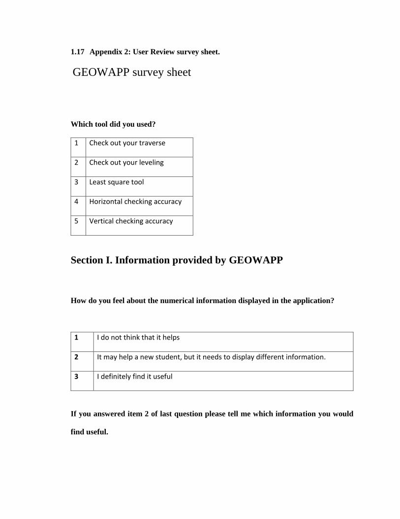
1.17 Appendix 2: User Review survey sheet.
GEOWAPP survey sheet
Which tool did you used?
1 Check out your traverse
2 Check out your leveling
3 Least square tool
4 Horizontal checking accuracy
5 Vertical checking accuracy
Section I. Information provided by GEOWAPP
How do you feel about the numerical information displayed in the application?
1 I do not think that it helps
2 It may help a new student, but it needs to display different information.
3 I definitely find it useful
If you answered item 2 of last question please tell me which information you would
find useful.

In terms of self-evaluation, would you feel more comfortable if you get this
information when you are in the field making measurement
1 No, I would feel the same
2 Probably, I am not really sure about it
3 I definitely would feel more comfortable if I can review the measurement while I
am in the field.
Section II. Geospatial web tool part (if you used any of the leveling tools
please past to the next section)
If you were a new student, would it help to visualize more effectively your work on
the field?
1 Not at all
2 I probably would be confused as well
3 Yes, It would help me to visualized my work

4 It definitely will give me the concept of what I am doing in the field.
If you were looking to find where a blunder (gross error or a mistake) happened, this
tool will help to so more effectively.
1 Not at all
2 I probably wouldn’t know where the blunder is even if I see it.
3 Yes, it would help me to know the area where the blunder occurred
4 It definitely would help me to identify any gross error more easily.
Section III. About the concept.
What are your feelings about the concept of a Geospatial Web Application for
enhancing survey labs?
1 Bad idea, not very useful
2 Interesting but not applicable
3 Really interesting and technologically advanced
4 Useful, interesting and very technologically advanced
Section IV. Your comments.
If you have comments or ideas about the tool or suggested changes/improvement,
please write them down.

1.18 User Guide
1.18.1 Register
1. Click on register
2. Input your information (see Figure Tut 1)
Figure Tut 1: the register window.
** note: all registered users are by default student. If an instructor account is needed
should be modified with an SQL statement: UPDATE users SET admin = 1 WHERE
`email`= "[email protected]";
Sign in:
1. Add your email and password.
2. Press the Sign in button. (see Figure Tut 2)
Figure Tut 2: Sign in window.
1.18.2 Traversing comparator:
1. Click on traversing

2. Click on check out traversing
3. Define the traverse type:
a. Starts in point A and Finishes in point B.
b. Start and finishes in point A in “Insert traverse type”
4. Define de number of observation. This option requires an integer number.
5. Click Submit
6. Insert angles, minutes, seconds, and distances.
7. Insert the code of the control points (see Step 3).
a. For option 3.a, type the code the initial station (ex. tst1)
b. For option 3.b, type the code of the initial and the final station (ex. tst1. tst2).
8. To show the map click in display traverse.
9. Check the checkboxes non-adjusted traverse and adjusted traverse to display the traverse
polygons.
Example: option 3.a, number observations = 7, initial station code = tst1:
Please insert the following data
Table Tut 1: Traversing data (units: meters).
from To deg min seg Dist
1 3 353 41 17 220.56
3 4 59 4 50 192.457
4 2 98 7 5 184.7
2 5 181 1 3 208.919
5 6 222 36 11 157.052
6 7 296 54 33 156.841
7 1 242 36 23 82.914
Point A tst1
** Point A has real coordinates in NB-stereographic projection and it is stored in the
database.

1.18.3 Leveling Comparator:
1. Click Leveling
2. Click in check out your leveling
3. Insert the number of forward turning point and the backwards turning points:
a. “Define the number of turning points for forward run”
b. “Define the number of turning points for return run”
4. Press submit
5. Insert the Benchmark codes: initial and final station (ex. BMMIL, BMOAK).
6. Insert the backsight readings, the forwardsight readings, and the distance between the rod
locations**.
** The distance between rod locations is optional. If no value is included, the
program assumed 1 km as the total levelling length.
Example:
a. BM1 = BMMIL
b. BM2= BMOAK
Insert the following data:
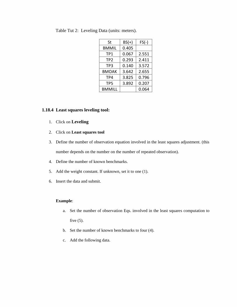
Table Tut 2: Leveling Data (units: meters).
1.18.4 Least squares leveling tool:
1. Click on Leveling
2. Click on Least squares tool
3. Define the number of observation equation involved in the least squares adjustment. (this
number depends on the number on the number of repeated observation).
4. Define the number of known benchmarks.
5. Add the weight constant. If unknown, set it to one (1).
6. Insert the data and submit.
Example:
a. Set the number of observation Eqs. involved in the least squares computation to
five (5).
b. Set the number of known benchmarks to four (4).
c. Add the following data.
St BS(+) FS(-)
BMMIL 0.405
TP1 0.067 2.551
TP2 0.293 2.411
TP3 0.140 3.572
BMOAK 3.642 2.655
TP4 3.825 0.796
TP5 3.892 0.207
BMMILL 0.064

Table Tut 3: Least squares data (units: meters).
From To Dist(km) Lev. Diff.(m)
BM1 A 2 10.997
BM2 A 2 -9.169
A B 0.5 3.532
BM3 B 1 4.858
BM4 B 1 -2.202
1 Bench mark code BM1
2 Bench mark code BM2
3 Bench mark code BM3
4 Bench mark code BM4
Weight Constant 1
1.18.5 Proximity Comparator:
1. Click on Horizontal Checking
2. Click on overall accuracy
3. In File, upload the csv file formatted like (ID,X,Y,code) (see Figure Tut 3).
Figure Tut. 3: csv format for the horizontal checking comparison (units: meters).
4. Select the sample name set by the instructor.
5. Then Submit.
6. Click on display accuracy polygons

7. Check the checkbox Tested point. These tested points are the sample stored in the
application.
8. Check the checkbox your survey points: This are the points you uploaded.
9. Analyze the information: a red pinpoint means that no point was found within the tolerance;
a green pinpoint means that a point was found within the tolerance)
10. Click on Download report
11. Look at the report. The report shows from the Id’s of the points and the distance within
points. At the end of this report, a RMS value is given.
Example:
Download a horizontal sample located in the main window.
Upload the downloaded file (make sure that the file name does not have a special
character like: “(), -, *, /, etc. ” ).
Choose sample_prox_1.csv in sample name.
Check the results.
Submit.
Vertical Comparator:
1. Click on Vertical Checking
2. Click on Vertical Accuracy
3. In File, Upload the file for processing. This csv file formatted like (ID,X,Y,Z) (see Figure
Tut 4).
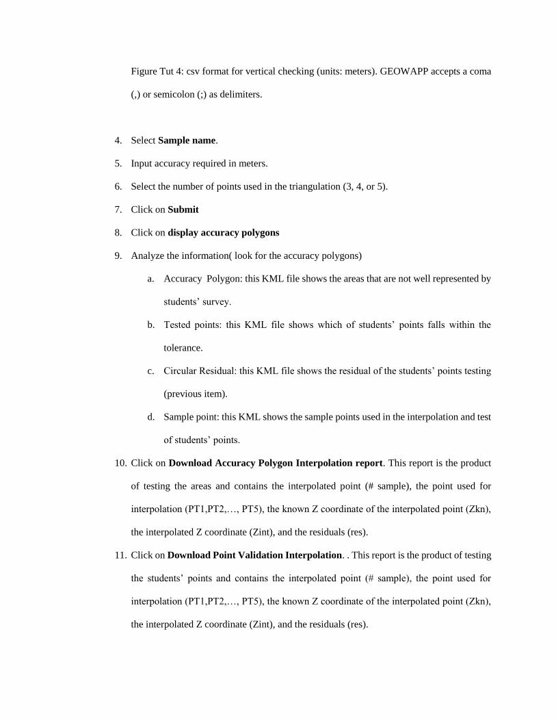
Figure Tut 4: csv format for vertical checking (units: meters). GEOWAPP accepts a coma
(,) or semicolon (;) as delimiters.
4. Select Sample name.
5. Input accuracy required in meters.
6. Select the number of points used in the triangulation (3, 4, or 5).
7. Click on Submit
8. Click on display accuracy polygons
9. Analyze the information( look for the accuracy polygons)
a. Accuracy Polygon: this KML file shows the areas that are not well represented by
students’ survey.
b. Tested points: this KML file shows which of students’ points falls within the
tolerance.
c. Circular Residual: this KML file shows the residual of the students’ points testing
(previous item).
d. Sample point: this KML shows the sample points used in the interpolation and test
of students’ points.
10. Click on Download Accuracy Polygon Interpolation report. This report is the product
of testing the areas and contains the interpolated point (# sample), the point used for
interpolation (PT1,PT2,…, PT5), the known Z coordinate of the interpolated point (Zkn),
the interpolated Z coordinate (Zint), and the residuals (res).
11. Click on Download Point Validation Interpolation. . This report is the product of testing
the students’ points and contains the interpolated point (# sample), the point used for
interpolation (PT1,PT2,…, PT5), the known Z coordinate of the interpolated point (Zkn),
the interpolated Z coordinate (Zint), and the residuals (res).
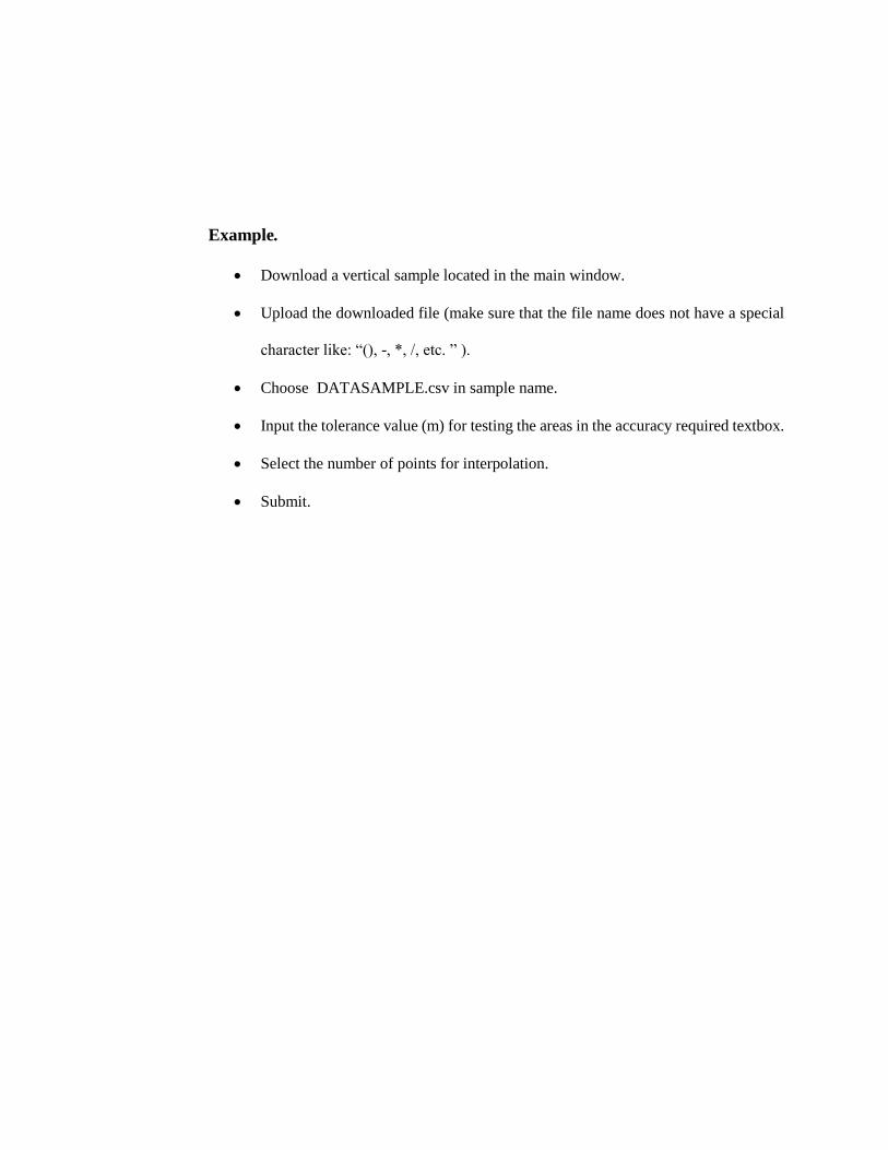
Example.
Download a vertical sample located in the main window.
Upload the downloaded file (make sure that the file name does not have a special
character like: “(), -, *, /, etc. ” ).
Choose DATASAMPLE.csv in sample name.
Input the tolerance value (m) for testing the areas in the accuracy required textbox.
Select the number of points for interpolation.
Submit.

Curriculum Vitae
Candidate’s full name: Jaime Garbanzo León
Universities attended: Universidad de Costa Rica, Costa Rica, 2004-2011
Degrees awarded: B. Eng. in Surveying Engineering, 2009.
Lic. Eng. in Surveying Engineering, 2012.