Embed Size (px)
Citation preview
A Geometric Analysis of Subspace Clusteringwith Outliers
Mahdi Soltanolkotabi and Emmanuel Candés
Stanford University

Fundamental Tool in Data Mining : PCA

Fundamental Tool in Data Mining : PCA

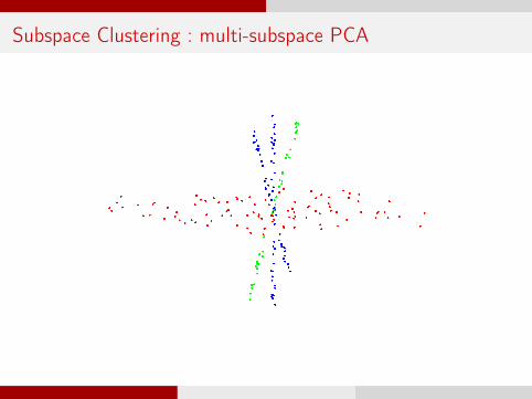
Subspace Clustering : multi-subspace PCA

Subspace Clustering : multi-subspace PCA
Subspace Clustering : multi-subspace PCA

Subspace Clustering : multi-subspace PCA

Subspace Clustering : multi-subspace PCA
Index
1 Motivation
2 Problem Formulation
3 Methods
4 Deterministic Model
5 Semi-random Model
6 Fully-random Model
7 With outliers

Motivation
1 Motivation
2 Problem Formulation
3 Methods
4 Deterministic Model
5 Semi-random Model
6 Fully-random Model
7 With outliers

Motivation
Computer Vision
Many applications.
Tuesday, January 10, 2012
Figures from various papers/talks.I refer to the interesting lecture by Prof. Ma tomorrow which highlights therelevance of low dimensional structures in computer vision. Just add multiplecategories :)

Motivation
Metabolic Screening
Goal Detect metabolic disease as early as possible in new borns.concentration of metabolites are tested.Usually, each metabolic disease causes a correlation between theconcentration of a specific set of metabolites.
Tuesday, January 10, 2012
Problem Formulation
1 Motivation
2 Problem Formulation
3 Methods
4 Deterministic Model
5 Semi-random Model
6 Fully-random Model
7 With outliers

Problem Formulation
Problem Formulation
N unit norm points in Rn on a union of unknown linear subspacesS1 ∪ S2 ∪ . . . ∪ SL of unknown dimensions d1, d2, . . . , dL. Also, N0
uniform outliers.
outliers inliers
Goal : Without any prior knowledge about the number of subspaces,their orientation or their dimension,1) identify all the outliers, and2) segment or assign each data point to a cluster as to recover all thehidden subspaces.

Methods
1 Motivation
2 Problem Formulation
3 Methods
4 Deterministic Model
5 Semi-random Model
6 Fully-random Model
7 With outliers
Methods
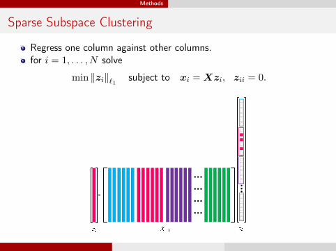
Sparse Subspace Clustering
Regress one column against other columns.for i = 1, . . . , N solve
min ‖zi‖`1 subject to xi = Xzi, zii = 0.
=
Methods
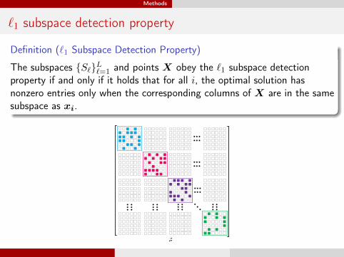
`1 subspace detection property
Definition (`1 Subspace Detection Property)
The subspaces {S`}L`=1 and points X obey the `1 subspace detectionproperty if and only if it holds that for all i, the optimal solution hasnonzero entries only when the corresponding columns of X are in the samesubspace as xi.

Methods
SSC Algorithm
Algorithm 1 Sparse Subspace Clustering (SSC)
Input: A data set X arranged as columns of X ∈ Rn×N .1. Solve (the optimization variable is the N ×N matrix Z)
minimize �Z��1subject to XZ =X
diag(Z) = 0.
2. Form the affinity graph G with nodes representing the N data points and edge weights givenby W = �Z � + �Z �T .3. Sort the eigenvalues σ1 ≥ σ2 ≥ . . . ≥ σN of the normalized Laplacian of G in descending order,and set
L̂ = N − argmaxi=1,...,N−1 σi − σi+1.
4. Apply a spectral clustering technique to the affinity graph using L̂.Output: Partition X1, . . . ,XL̂.
• Subspaces of nearly linear dimension. We prove that in generic settings, SSC caneffectively cluster the data even when the dimensions of the subspaces grow almost linearlywith the ambient dimension. We are not aware of other literature explaining why this shouldbe so. To be sure, in most favorable cases, earlier results only seem to allow the dimensionsof the subspaces to grow at most like the square root of the ambient dimension.
• Outlier detection. We present modifications to SSC that succeed when the data set iscorrupted with many outliers—even when their number far exceeds the total number of cleanobservations. To the best of our knowledge, this is the first algorithm provably capable ofhandling these many corruptions.
• Geometric insights. Such improvements are possible because of a novel approach to an-alyzing the sparse subspace clustering problem. This analysis combine tools from convexoptimization, probability theory and geometric functional analysis. Underlying our methodsare clear geometric insights explaining quite precisely when SSC is successful and when it isnot. This viewpoint might prove fruitful to address other sparse recovery problems.
Section 3 proposes a careful comparison with the existing literature. Before doing so, we first needto introduce our results, which is the object of Sections 1.4 and 2.
1.4 Models and typical results
1.4.1 Models
In order to better understand the regime in which SSC succeeds as well as its limitations, we willconsider three different models. Our aim is to give informative bounds for these models highlightingthe dependence upon key parameters of the problem such as 1) the number of subspaces, 2) thedimensions of these subspaces, 3) the relative orientations of these subspaces, 4) the number ofdata points per subspace, and so on.
5

Methods
History of subspace problems and use of `1 regression
Various subspace clustering algorithms proposed by Profs. Ma, Sastry,Vidal, Wright and collaborators.
Sparse representation in the multiple subspace framework initiated byProf. Yi Ma and collaborators in the context of face recognition.
Different from subspace clustering because you know the subspaces inadvance.
For subspace clustering by Elhamifar and Vidal. Coined the nameSparse Subspace Clustering (SSC).
Methods
History of subspace problems and use of `1 regression
Various subspace clustering algorithms proposed by Profs. Ma, Sastry,Vidal, Wright and collaborators.Sparse representation in the multiple subspace framework initiated byProf. Yi Ma and collaborators in the context of face recognition.
Different from subspace clustering because you know the subspaces inadvance.
For subspace clustering by Elhamifar and Vidal. Coined the nameSparse Subspace Clustering (SSC).
Methods
Our goal
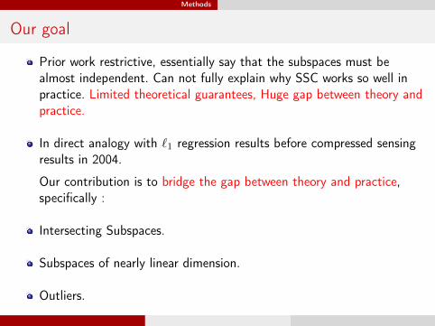
Prior work restrictive, essentially say that the subspaces must bealmost independent. Can not fully explain why SSC works so well inpractice. Limited theoretical guarantees, Huge gap between theory andpractice.
In direct analogy with `1 regression results before compressed sensingresults in 2004.
Our contribution is to bridge the gap between theory and practice,specifically :
Intersecting Subspaces.
Subspaces of nearly linear dimension.
Outliers.
Geometric Insights.

Methods
Our goal
Prior work restrictive, essentially say that the subspaces must bealmost independent. Can not fully explain why SSC works so well inpractice. Limited theoretical guarantees, Huge gap between theory andpractice.
In direct analogy with `1 regression results before compressed sensingresults in 2004.
Our contribution is to bridge the gap between theory and practice,specifically :
Intersecting Subspaces.
Subspaces of nearly linear dimension.
Outliers.
Geometric Insights.
Methods
Models
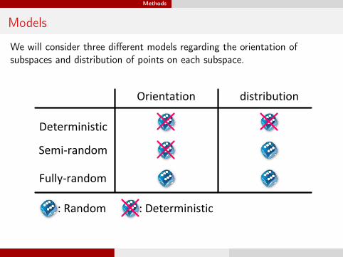
We will consider three different models regarding the orientation ofsubspaces and distribution of points on each subspace.
Fully-random
Semi-random
Deterministic
Orientation distribution
: Random : Deterministic

Deterministic Model
1 Motivation
2 Problem Formulation
3 Methods
4 Deterministic Model
5 Semi-random Model
6 Fully-random Model
7 With outliers
Deterministic Model
Deterministic Model
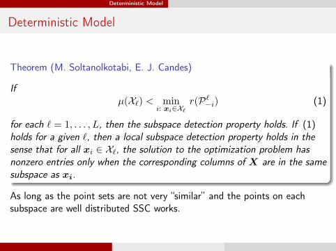
Theorem (M. Soltanolkotabi, E. J. Candes)
Ifµ(X`) < min
i: xi∈X`r(P`−i) (1)
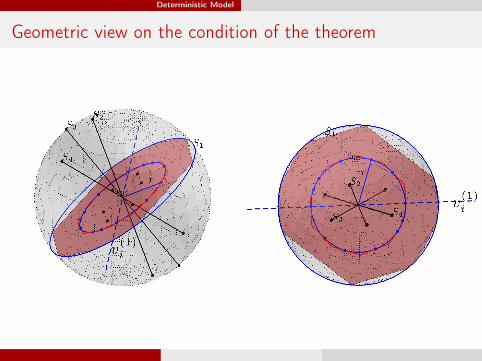
for each ` = 1, . . . , L, then the subspace detection property holds. If (1)holds for a given `, then a local subspace detection property holds in thesense that for all xi ∈ X`, the solution to the optimization problem hasnonzero entries only when the corresponding columns of X are in the samesubspace as xi.
As long as the point sets are not very “similar” and the points on eachsubspace are well distributed SSC works.
Deterministic Model
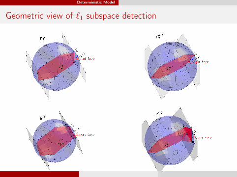
Geometric view of `1 subspace detection
Deterministic Model
Geometric view on the condition of the theorem
Semi-random Model
1 Motivation
2 Problem Formulation
3 Methods
4 Deterministic Model
5 Semi-random Model
6 Fully-random Model
7 With outliers

Semi-random Model
principal angle and affinity between subspaces
Definition
The principal angles θ(1)k,` , . . . , θ(dk
∨d`}
k,` between two subspaces Sk and S`of dimensions dk and d`, are recursively defined by
cos(θ(i)k` ) = max
y∈Skmaxz∈S`
yTz
‖y‖`2 ‖z‖`2=
yTi zi‖yi‖`2 ‖zi‖`2
.
with the orthogonality constraints yTyj = 0, zTzj = 0, j = 1, . . . , i− 1.
DefinitionThe affinity between two subspaces is defined by
aff(Sk, S`) =√cos2 θ
(1)k` + . . .+ cos2 θ
(dk∨d`)
k` .
For random subspaces square of affinity is the Pillai-Bartlett test Statistics.

Semi-random Model
Semi-random model
Assume we have N` = ρ`d` + 1 random points on subspace S`.
Theorem (M. Soltanolkotabi, E. J. Candes)
Ignoring some log factors, as long as
maxk : k 6=`
aff(Sk, S`)√dk
< c√log ρ`, for each `, (2)
the subspace detection property holds with high probability.
The affinity can at most be√dk and, therefore, our result essentially
states that if the affinity is less than c√dk, then SSC works.
allows for intersection of subspaces.

Semi-random Model
Four error criterion
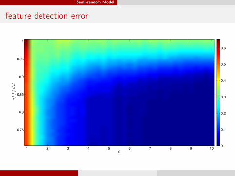
feature detection error : For each point xi in subspace S`i wepartition the optimal solution of SSC (zi) in the form
zi = Γ
zi1zi2zi3
.
1
N
N∑i=1
(1−‖ziki‖`1‖zi‖`1
).
clustering error :
# of misclassified pointstotal # of points
.
Semi-random Model
Four error criterion
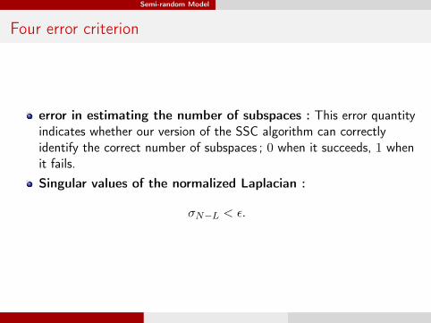
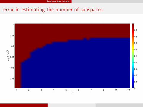
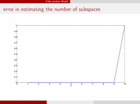
error in estimating the number of subspaces : This error quantityindicates whether our version of the SSC algorithm can correctlyidentify the correct number of subspaces ; 0 when it succeeds, 1 whenit fails.Singular values of the normalized Laplacian :
σN−L < ε.
Semi-random Model
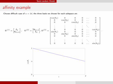
affinity exampleChoose difficult case of n = 2d, the three basis we choose for each subspace are
U(1)
=
[Id
0d×d
], U
(2)=
[0d×dId
],U
(3)=
cos(θ1) 0 0 0 . . . 00 cos(θ2) 0 0 . . . 00 0 cos(θ3) 0 . . . 0
.
.
....
.
.
....
. . ....
0 0 0 0 . . . cos(θd)sin(θ1) 0 0 0 . . . 0
0 sin(θ2) 0 0 . . . 00 0 sin(θ3) 0 . . . 0
.
.
....
.
.
....
. . ....
0 0 0 0 . . . sin(θd)
.
i
cos!
i
"
1
d10
Semi-random Model
feature detection error
!
aff/!d
1 2 3 4 5 6 7 8 9 10
0.75
0.8
0.85
0.9
0.95
1
0
0.1
0.2
0.3
0.4
0.5
0.6

Semi-random Model
clustering error
!
aff/!d
1 2 3 4 5 6 7 8 9 10
0.75
0.8
0.85
0.9
0.95
1
0
0.1
0.2
0.3
0.4
0.5
0.6
Semi-random Model
error in estimating the number of subspaces
!
aff/!d
1 2 3 4 5 6 7 8 9 10
0.75
0.8
0.85
0.9
0.95
1
0
0.1
0.2
0.3
0.4
0.5
0.6
0.7
0.8
0.9
1
Fully-random Model
1 Motivation
2 Problem Formulation
3 Methods
4 Deterministic Model
5 Semi-random Model
6 Fully-random Model
7 With outliers

Fully-random Model
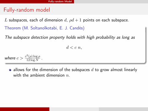
Fully-random model
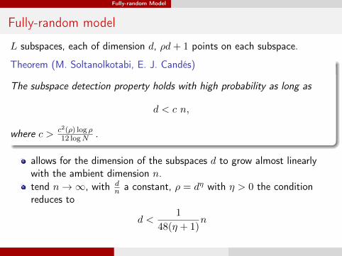
L subspaces, each of dimension d, ρd+ 1 points on each subspace.
Theorem (M. Soltanolkotabi, E. J. Candés)
The subspace detection property holds with high probability as long as
d < c n,
where c > c2(ρ) log ρ12 logN .
allows for the dimension of the subspaces d to grow almost linearlywith the ambient dimension n.tend n→∞, with d
n a constant, ρ = dη with η > 0 the conditionreduces to
d <1
48(η + 1)n
Fully-random Model
Fully-random model
L subspaces, each of dimension d, ρd+ 1 points on each subspace.
Theorem (M. Soltanolkotabi, E. J. Candés)
The subspace detection property holds with high probability as long as
d < c n,
where c > c2(ρ) log ρ12 logN .
allows for the dimension of the subspaces d to grow almost linearlywith the ambient dimension n.
tend n→∞, with dn a constant, ρ = dη with η > 0 the condition
reduces to
d <1
48(η + 1)n
Fully-random Model
Fully-random model
L subspaces, each of dimension d, ρd+ 1 points on each subspace.
Theorem (M. Soltanolkotabi, E. J. Candés)
The subspace detection property holds with high probability as long as
d < c n,
where c > c2(ρ) log ρ12 logN .
allows for the dimension of the subspaces d to grow almost linearlywith the ambient dimension n.tend n→∞, with d
n a constant, ρ = dη with η > 0 the conditionreduces to
d <1
48(η + 1)n
Fully-random Model
Comparison with previous analysis
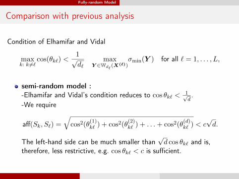
Condition of Elhamifar and Vidal
maxk: k 6=`
cos(θk`) <1√d`
maxY ∈Wd`
(X(`))σmin(Y ) for all ` = 1, . . . , L,
semi-random model :-Elhamifar and Vidal’s condition reduces to cos θk` <
1√d.
-We require
aff(Sk, S`) =√cos2(θ
(1)k` ) + cos2(θ
(2)k` ) + . . .+ cos2(θ
(d)k` ) < c
√d.
The left-hand side can be much smaller than√d cos θk` and is,
therefore, less restrictive, e.g. cos θk` < c is sufficient.
Fully-random Model
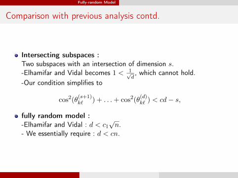
Comparison with previous analysis contd.
Intersecting subspaces :Two subspaces with an intersection of dimension s.-Elhamifar and Vidal becomes 1 < 1√
d, which cannot hold.
-Our condition simplifies to
cos2(θ(s+1)k` ) + . . .+ cos2(θ
(d)k` ) < cd− s,
fully random model :-Elhamifar and Vidal : d < c1
√n.
- We essentially require : d < cn.

Fully-random Model
Subspaces Intersect
s = 1 s = 2
s = 3 s = 4

Fully-random Model
feature detection error
0 1 2 3 4 5 6 7 8 9 100
0.1
0.2
0.3
0.4
0.5
0.6
0.7
0.8
0.9
1
s
Fully-random Model
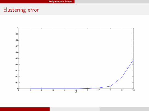
clustering error
0 1 2 3 4 5 6 7 8 9 100
0.1
0.2
0.3
0.4
0.5
0.6
0.7
0.8
0.9
1
s
Fully-random Model
error in estimating the number of subspaces
0 1 2 3 4 5 6 7 8 9 100
0.1
0.2
0.3
0.4
0.5
0.6
0.7
0.8
0.9
1
s

With outliers
1 Motivation
2 Problem Formulation
3 Methods
4 Deterministic Model
5 Semi-random Model
6 Fully-random Model
7 With outliers
With outliers
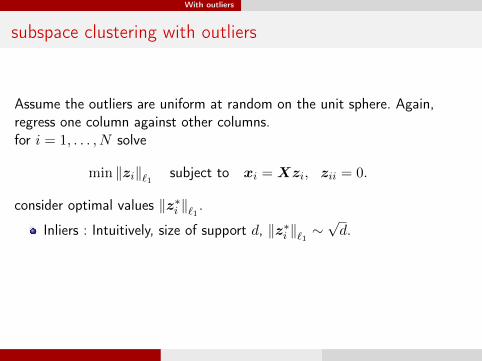
subspace clustering with outliers
Assume the outliers are uniform at random on the unit sphere. Again,regress one column against other columns.for i = 1, . . . , N solve
min ‖zi‖`1 subject to xi = Xzi, zii = 0.
consider optimal values ‖z∗i ‖`1 .
Inliers : Intuitively, size of support d, ‖z∗i ‖`1 ∼√d.
Outliers : Intuitively, size of support n, ‖z∗i ‖`1 ∼√n.
Therefore, we should expect a gap.
With outliers
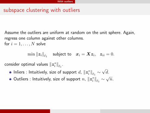
subspace clustering with outliers
Assume the outliers are uniform at random on the unit sphere. Again,regress one column against other columns.for i = 1, . . . , N solve
min ‖zi‖`1 subject to xi = Xzi, zii = 0.
consider optimal values ‖z∗i ‖`1 .
Inliers : Intuitively, size of support d, ‖z∗i ‖`1 ∼√d.
Outliers : Intuitively, size of support n, ‖z∗i ‖`1 ∼√n.
Therefore, we should expect a gap.
With outliers
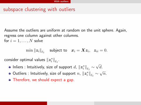
subspace clustering with outliers
Assume the outliers are uniform at random on the unit sphere. Again,regress one column against other columns.for i = 1, . . . , N solve
min ‖zi‖`1 subject to xi = Xzi, zii = 0.
consider optimal values ‖z∗i ‖`1 .
Inliers : Intuitively, size of support d, ‖z∗i ‖`1 ∼√d.
Outliers : Intuitively, size of support n, ‖z∗i ‖`1 ∼√n.
Therefore, we should expect a gap.

With outliers
Inliers : Intuitively, size of support d, ‖z∗i ‖`1 ∼√d. Here,
‖z∗i ‖`1 = 1.05.
Outliers : Intuitively, size of support n, ‖z∗i ‖`1 ∼√n. Here,
‖z∗i ‖`1 = 1.72.

With outliers
Inliers : Intuitively, size of support d, ‖z∗i ‖`1 ∼√d. Here,
‖z∗i ‖`1 = 1.05.
Outliers : Intuitively, size of support n, ‖z∗i ‖`1 ∼√n. Here,
‖z∗i ‖`1 = 1.72.

With outliers
Algorithm for subspace clustering with outliers[M. Soltanolktoabi, E. J. Candes]
Algorithm 2 Subspace clustering in the presence of outliers
Input: A data set X arranged as columns of X ∈ Rn×N .1. Solve
minimize �Z��1subject to XZ =X
diag(Z) = 0.
2. For each i ∈ {1, . . . ,N}, declare i to be an outlier iff �zi��1 > λ(γ)√n.3
3. Apply a subspace clustering to the remaining points.Output: Partition X0,X1, . . . ,XL.
Theorem 1.3 Assume there are Nd points to be clustered together with N0 outliers sampled uni-formly at random on the n − 1-dimensional unit sphere (N = N0 +Nd). Algorithm 2 detects all ofthe outliers with high probability4 as long as
N0 < 1
nec√
n −Nd,
where c is a numerical constant. Furthermore, suppose the subspaces are d-dimensional and ofarbitrary orientation, and that each contains ρd + 1 points sampled independently and uniformlyat random. Then with high probability,5 Algorithm 2 does not detect any subspace point as outlierprovided that
N0 < nρc2nd −Nd
in which c2 = c2(ρ)�(2e2π).This result shows that our outlier detection scheme can reliably detect all outliers even when
their number grows exponentially in the root of the ambient dimension. We emphasize that thisholds without making any assumption whatsoever about the orientation of the subspaces or thedistribution of the points on each subspace. Furthermore, if the points on each subspace areuniformly distributed, our scheme will not wrongfully detect a subspace point as an outlier. In thenext section, we show that similar results hold under less restrictive assumptions.
2 Main Results
2.1 Segmentation without outliers
In this section, we shall give sufficient conditions in the fully deterministic and semi-random modelunder which the SSC algorithm succeeds (we studied the fully random model in Theorem 1.2).
Before we explain our results, we introduce some basic notation. We will arrange the N� points
on subspace S� as columns of a matrix X(�). For � = 1, . . . , L, i = 1, . . . ,N�, we use X(�)−i to
denote all points on subspace S� excluding the ith point, X(�)−i = [x(�)1 , . . . ,x
(�)i−1,x(�)i+1, . . . ,x(�)N�
]. We
use U (�) ∈ Rn×d� to denote an arbitrary orthonormal basis for S�. This induces a factorization
4With probability at least 1 −N0e−Cn� log�2(N0+Nd)�. If N0 < 1
nec√
n −Nd, this is at least 1 − 1n.
5With probability at least 1 − N0e−Cn� log�2(N0+Nd)� − Nde−√ρd. If N0 < min{nec2
nd , 1
nec√
n} − Nd, this is at least
1 − 1n−Nde−√ρd.
8
2 γ = N−1n and λ is a threshold ratio function.
With outliers
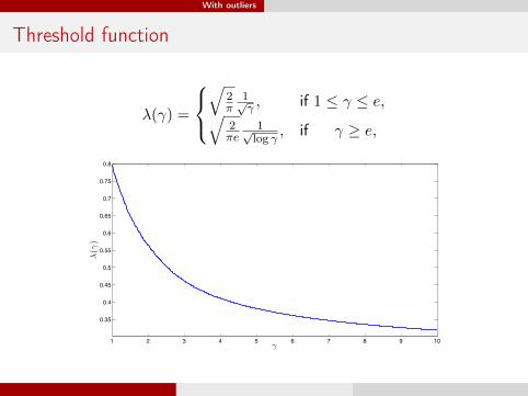
Threshold function
λ(γ) =
√
2π
1√γ , if 1 ≤ γ ≤ e,√
2πe
1√log γ
, if γ ≥ e,
1 2 3 4 5 6 7 8 9 10
0.35
0.4
0.45
0.5
0.55
0.6
0.65
0.7
0.75
0.8
!
"(!
)
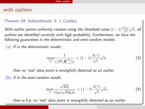
With outliers
with outliers
Theorem (M. Soltanolkotabi, E. J. Candés)
With outlier points uniformly random using the threshold value (1− t)λ(γ)√e
√n, all
outliers are identified correctly with high probability. Furthermore, we have thefollowing guarantees in the deterministic and semi-random models.
(a) If in the deterministic model,
max`,i
1
r(P(X(`)−i ))
< (1− t)λ(γ)√e
√n, (3)
then no ‘real’ data point is wrongfully detected as an outlier.
(b) If in the semi-random model,
max`
√2d`
c(ρ`)√log ρ`
< (1− t)λ(γ)√e
√n, (4)
then w.h.p. no ‘real’ data point is wrongfully detected as an outlier.
With outliers
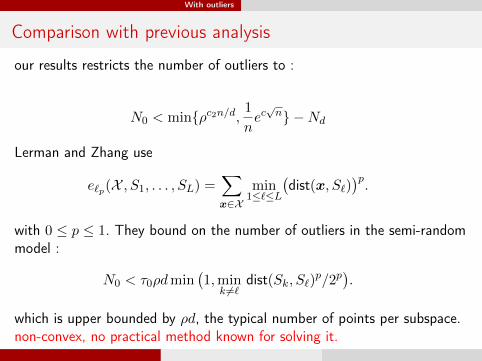
Comparison with previous analysis
our results restricts the number of outliers to :
N0 < min{ρc2n/d, 1nec√n} −Nd
Lerman and Zhang use
e`p(X , S1, . . . , SL) =∑x∈X
min1≤`≤L
(dist(x, S`)
)p.
with 0 ≤ p ≤ 1. They bound on the number of outliers in the semi-randommodel :
N0 < τ0ρdmin(1,min
k 6=`dist(Sk, S`)p/2p
).
which is upper bounded by ρd, the typical number of points per subspace.non-convex, no practical method known for solving it.
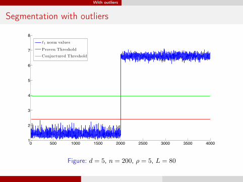
With outliers
Segmentation with outliers
0 500 1000 1500 2000 2500 3000 3500 40001
2
3
4
5
6
7
8!1 norm values
Proven Threshold
Conjuctured Threshold
Figure: d = 5, n = 200, ρ = 5, L = 80

With outliers
References
List is not comprehensive !A geometric analysis of subspace clustering. M. Soltanolkotabi andE. J. Candes to appear in Annals of Statistics.Noisy case, in preparation. Joint with E. J. Candes, E. Elhamifar, andR. Vidal.www.stanford.edu/~mahdisol.Sparse Subspace Clustering. E. Elhamifar and R. Vidal.Subspace Clustering. Turorial by R. Vidal.Prof. Yi Ma’s website for papers on related topics :http://yima.csl.illinois.edu/.

With outliers
Conclusion
Prior work restrictive, essentially say that the subspaces must bealmost independent. Can not fully explain why SSC works so well inpractice.
In direct analogy with `1 regression results before compressed sensingresults in 2004.
Our contributions is to bridge the gap between theory and practice,specifically :
Intersecting Subspaces.
Subspaces of nearly linear dimension.
Outliers.
Geometric Insights.

With outliers
Thank you

![Beyond outliers and on to micro-clusters: Vision-guided ...For graph anomaly detection, [30,21] nd communities and suspicious clusters with spectral-subspace plots. SpokEn[30] considers](https://img.pdfslide.us/doc/110x75/5f47770af15dfb4e8b6989af/beyond-outliers-and-on-to-micro-clusters-vision-guided-for-graph-anomaly-detection.jpg)