A Generalization of Whittaker-Henderson Graduation - Society of

TRANSACTIONS OF SOCIETY OF ACTUARIES 1 9 8 4 VOL. 36

A GENERALIZATION OF WHITTAKER-HENDERSON GRADUATION

FUNG YEE C H A N , LAI K. C H A N , * AND M A N HEI YU**

ABSTRACT

The Whittaker-Henderson graduation method of minimizing F + h S with fit F of the form Z W x l U x - U ' ~ ° and smoothness S of the form y l X-'u2' is investigated for 1 < p -< ~. It is shown that for a given h, the set of graduated values u ~ = (u] . . . . . u~) r is unique and is the solution of the system of equations F ' (u) + h S ' ( u ) = 0 r w h e n 1 < p < ~ , a n d u x is an optimal solution of an equivalent linear programming problem when p = ~. Algo- rithms for computing u ~ = (u~ . . . . . u~) r are proposed. The graduated values for different p are compared. Some properties of F(u~), S (u h) and F ( u ~ ) + h S ( u ~) are obtained. The modification to the minimization of F (or S) when S (or F) is constrained to be less than or equal to a predetermined number is proposed and studied.

1. INTRODUCTION

Given a vector of ungraduated (that is, observed) values u" (u'; . . . . ,u~) r and a constant h -> 0, the Whittaker-Henderson ~aduation method finds the optimum values u ~' = (u~ . . . . . u~) r, called the graduated values, which minimize

F ( u ) + kS(u) over all u =- (u l . . . . . u,,) r,

where F is a measure of the fit of u to u" and S is a measure of the smoothness of the values in u.

The well-known Whittaker-Henderson Type B method presented in the

* Dr. Chan, not a member of the Society, is Professor and Head, Department of Statistics, University of Manitoba, Canada.

** Mr. Yu, not a member of the Society, is a graduate student in the Department of Actuarial and Management Sciences, University of Manitoba, Canada.

183

1 8 4 G E N E R A L I Z A T I O N O F W H I T T A K E R - H E N D E R S O N G R A D U A T I O N

Society of Actuaries Part 5 Study Notes by Greville [5, pp. 49-54] uses the square of the e2-norms:

n n ~ z

F ( u ) - ~ ~ wx(u~-Ux) 2 and S(u)-=- ~] (AZux) 2, x = l x = l

where the wx > 0 are the weights assigned to the u", and the AZux are the zth differences of Ux. The formula for the graduated values is obtained elegantly by Greville [5, pp. 49-54] using linear algebra and by Shiu [15] using advanced calculus.

Schuette [14] used the el-norms: n - - Z

F ( u ) = WxlU" - uxl and S ( u ) - • IA%I x = l x = l

and showed that u x can be obtained by formulating the problem as a linear programming problem.

In Section 2 of this paper, the general case of the ep-norms is solved: t I - - Z

F ( u ) ----- wxlu"- ux~' and S(u) - ~ [A%,I p x = l x = l

with 1 < p < ~ . In the discussion of Schuette's paper [14], Professor Greville [6] sug-

gested that " i t would be most interesting and worthwhile if someone would perform the same task for the Chebyshev norm that Schuette has done for the e l -norm."

Before proceeding to the case p = ~, we digress to discuss the definition of the ep-norm. The definition of norm is given by Schuette [14]. If y =

'(Yl, - • • ,Y,,) is a vector of real or complex numbers, then the ep-nor~a of "the vector, denoted by Ilyll,,, is defined as

Ilyllp = ( [ y l F ° + . . . + [YnlP) '/p for 1 --< p < ~. For the case p = 0% the e~-norm or Chebyshev norm (also called the uniform norm) is defined as

II Y IL = max ly l.

It is intuitively clear and can be shown analytically that the following property holds [cf. 10, p. 248]

lim II Y lip -- Ily I1=

The term F ( u ) -- ~] wxlu~, - u"~ is the pth power of the weighted norm X = I

n - - z

of ux - u~ with weights w x, and S(u) --- ~] ]A~ux~ is the pth power of x = l

GENERALIZATION OF WHITTAKER-HENDERSON GRADUATION 185

the norm of AZux . Therefore, in the e=-norm case, F ( u ) and S(u) should be defined as:

F ( u ) = max ]Ux- Uxl and S( u ) = max lazuxl.

The weights w~ disappear in the term F ( u ) since

l im(~] wxlu~-u"~°) 'In = max lux-u"l p ~ o o x = 1 I ~ x ~ n

which can be seen from the property indicated earlier. In section 3 of this paper the ~e:norm problem suggested by Greville [6]

is solved by formulating it as a linear programming problem. At that point, the problem of obtaining graduated values for the well-known Whit- taker-Henderson graduation method will have been solved for all ep-norms with 1 -<p-<oo.

The e=-norm case is further generalized to include the weights w~, for example,

F ( u ) -- max w~]u~ - u"[. 1 ~ x ~ n

The term max wxlux - u~] is a weighted C-norm of u - ~ ' , although it

does not have the property that

l im(~] WxlU~-U"~) lie = max wxl~x-u"l. P ~ x = 1 I ~ x ~ n

Although the u~ are usually nonnegative in actuarial applications, we allow them to be negative in our studies. Minimizing a nonlinear function of several variables under constraints is theoretically and computationally com- plicated, because the optimal solution may occur on the boundary (for example, Ux ~ = 0 for some x). In practice, when the ungraduated values u" are positive, the graduated values u~ will usually be positive even when the nonnegative constraints are not imposed on the Ux.

In Section 4, it is shown that the solutions have the Monotone Properties:

F( u ~) + hS( u ~) is a nondecreasing function of X F( u.. ~) is a nondecreasing function of h S( u ~) is a nonincreasing function of h

in fact, for 1 < p < o% F ( u ~) and F ( u ~) + h S ( u ~) are increasing and S ( u ~) is decreasing, provided that S ( u ~) > O.

Furthermore, (F(uX), S(u~)) is Pareto-optimal (see Gerber [4], 91):

There does not exist u such that

186 GENERALIZATION OF WHI'ITAKER-HENDERSON GRADUATION

F ( u ) <~ F ( u ~) and S ( u ) ~ S ( u ~) with at

least one inequality being strict.

Numerical examples are given in Section 5, in which graduated values obtained using different p are compared.

Lowrie [11] extended F and included exponential smoothness in S. In the discussion of Lowrie's paper, Chan, Chan and Mead [2] showed that the extension also has the Monotone Properties and is Pareto-optimal.

The Whittaker-Henderson graduation method [16] has a Bayesian statistical interpretation, which has been advanced by Hickman and Miller [7, 8].

Modifications of the graduation problem to the problems

Min F(u) under the constraint S(u) ~< c u

and

Min S(u) under the constraint F(u) ~< c, u

where c > 0 is a given constant, are given in Section 6. Lemmas and theorems which require longer proofs are given in the ap-

pendices.

2. -~p-NORM WITH 1 < p <

Let 1 < p < ~ and h /> 0 be given constants. Consider the following problem:

Min[F(u) + kS(u)] (WH) tt

where t l - - z

F ( u ) =- w, [ Ux - u:" ~' and S(E) ~ E I AZux I p. x = l x = l

We proceed to show that the optimal solution u~ = (u~ . . . . . ug)T to (WH) is the unique solution of the system of equations

F'(u) + hS'(u~ = O. T (2.1)


LEMMA 2. l" F ( u ) and S( u ) are differentiable at every point u ~ R '~. They are twice differentiable except when u x = u~ or AZux = 0 for some x f o r 1 < p < 2, and

(i) f ' ( u ) -- Oul . . . . .

s ' ( u ) - . . . . .

= p[lu, - uT IP - I s g n ( u l - uT) . . . . .

lu. - u " l~ ' -~ sgn(u , , - u D l W

= p t l a = u , I ~ , - ' s g n ( A = u , ) . . . . .

IA=u,_=~"-lsgn(A=u,_=)]K,

where W is the n x n diagonal matrix with diagonal elements w I . . . . . w,, and K is the ( n - z ) x n zth differencing matrix, i.e., K u is the column vector (A-'uj . . . . . AZu,_~)r, and

1 i f x > O , sgn(x) = 0 / fx = 0,

- 1 / fx < 0.

(ii)

u,-u~'~ -2 0 21 ro2F1 " . " " • , , o W

F ' ( u ) - LauiauJJ = p (p- ]) 0 "1;.~,- u~t.-

C " i ' " " " K S"(u) =- [ . ~ j = p ( p - 1)K r "l&'~k,,-~ -2

Proof. See Appendix I(a). It is clear from (ii) that S"(u) and F" (u ) are nonnegative definite if they

exist. Therefore, F" (u ) + hS" (u ) is nonnegative definite for every u , and hence F + kS is convex on R".

In fact, since Ix[ p is a strictly convex function, we have

LEMMA 2.2: F + XS is strictly convex on R ~.

Proof. See Appendix I(b). Based on a documented property of a strictly convex function of several

variables [3, §2.1], we have

188 GENERALIZATION OF WHITrAKER-HENDERSON GRADUATION

THEOREM 2.1: For a given h >- O, u ~ is an optimal solution to (WH) i f and only i f F ' ( u ~) + h S ' ( u ~) = O. Furthermore, this optimal solution is unique.

Since F + kS is strictly convex, the following Newton-Raphson algorithm [12, p.288] is used for solving the system of equations (2.1).

THEOREM 2.2: Let u ° be an initial value and u k denote the value after k iterations. I f we set

u k+l --- u k -- [F" ( u.~ k) + kS"( u...k)]- ' [F ' ( u k) + kS' ( u k)] T,

and it converges to u , then u is the unique solution o f equation (2.1) provided that f o r each k, IF" (..~k) + kS" (uk)] - I exists.

Whenp > 2, F" ( u k) + kS" ( u k) is nonsingular i fF" ( u k) is nonsingular, which can be achieved if ~ 4: u" for all x = 1 . . . . . n. So, in case u~-u~ = 0 for some x, we can always change u~ to u~ + • with • 4: O.

For the case p = 2, Greville's [5] graduated values can be obtained immediately from Theorem 2.2. Since

[F'(u.u) + kS' (u~] r = 2W(u - u-') + 2hKTKu,

and

F" ( u ) + h S " ( u ) = 2 W + 2hKTK,

and the latter is positive definite and, hence, nonsingular, then for any u °,

u ' = u ° - [F" ( u °) + kS" ( u ° ) l - l [ F ' ( u °) + hS' (u°)] r = u o - [ 2 W + 2 X K r K ] - ~ I 2 W ( u O - u '~) - 2 X K ' r K ( u O ) ] = u o - [ W + X K r K ] - ~ [ ( W + X l f r K ) ( u o ) - W u " ]

= u o - u o + ( W + M f r K ) - l W u "

"Cw + x h3 - ' W u" ,

which is independent of u o. tt Z k For 1 < p < 2 , u~ = Ux or A Ux = 0 for some x will lead to infinity in the

entries of F" ( u k) or S" (uk); that is, F" ( u k) + ks" ( u k) and [F" ( u k) + ks,, (uk) ] - 1 do not exist.

An APL program is written for carrying out the iterations in Theorem 2.2 and is given in Appendix I(b).

Usually F" ( u k) + kS" ( u k) is a large matrix. Therefore, the square-root method or Choleski method (which can be found in Greville [5]) is rec- ommended for finding u k÷~ We can find u k÷l by using the above method


to solve [F" ( u k) + hS" (uk)] u k+t = [F" ( u k) + kS" (Uk)] U k -- [F' ( u k) + hS' (uk)] instead of inverting F" ( u k) + hS" (u~).

3. e~-NORM

In this section, we solve the e~-norm problem raised by Greville [6] by formulating it as a linear programming problem.

The problem then is

Min [F (u) + hS(u)l ~ o -- (WH)

where

F ( u ) ~ max w lux-u l and S ( u ) - max I a % l . 1 ~ x ~ n 1 ~ x ~ n - z

We will consider the more general form of F ( u ) , that is,

F( u ) - m a x wx l u:l, I ~x~n

which has F ( u ) -- max lux-u~l as a special case. 1 ~ . x ~ n

THEOREM 3.1" Let h and wl . . . . . w n be given constants. The Whittaker- Henderson graduation method with (oo - norm (WH)and u >- 0 is equivalent to the linear programming problem, whose optimal solution always exists,

of:

Min (f+ ks) (LP) ~.l .s

under the constraints

WxUx - wxu"--<f, 1 x = 1 . . . . . n,

-WxUx + w~u~ <-- f ,

U,kxi s, } i=l

x = 1 , . . . , n - z ,

-- ~ uikxi ~ s, i=l

(3.1 a)

(3. I b)

190 G E N E R A L I Z A T I O N O F V C H I T T A K E R - H E N D E R S O N G R A D U A T I O N

ul . . . . . un, f , s >- O,

where [kxi ] = K is the zth difference matrix. I f ( u ~, fx, sx) is an optimal solution to (LP), then u ~ is an optimal solution to (WH) and

f~ = F ( u ~) and sx = S(uX).

Proof. See Appendix II. If the Ux are not constrained to be nonnegative in the (LP) formulation,

they can be replaced by Ux = U x - ux , where u~ -> 0 and u x -> 0. Linear programming is the most widely used mathematical optimization

model in operations research. Its optimal solution can be easily obtained by the simplex method. More about linear programming can be found in the Society of Actuaries Part 3 Examination reference, Hillier and Lieberman [9].

Since the optimal solution of (LP) and, hence, that of (WH) may not be unique, the first optimal solution obtained after the linear programming may not be a good fit to u . We can improve the goodness of fit of the solution by using quadratic programming. For example, suppose we have obtained u ~ as an optimal solution and that F(u) + hS(u) = M. We can then formulate the quadratic programming problem

Min ~ w~(u x - u") 2 (QP) u , f , s x = l

under the constraints (3. la), (3. lb) and the additional constraint

f + k s < - M .

It can be easily seen that any solution of (QP) is a solution of (WH). However, for the case with wx = 1 in F(u), the optimal solution obtained

at the end of the linear programming is close to u" (though it may not be unique), and no further quadratic programming is needed.

Another advantage of formulating (WH) as a linear programming problem is that one can perform sensitivity analyses. This is analyzing the effects on the optimal solution (uh, f~, s~) of one or more of the following changes:

h---~h + ~h

tr rt t t

U x ~ U x + ~U x

Wx---~ w~ + ~w x.


The computational procedures for doing this analysis are given in [9, §5.3]. They are based on the final simplex tableau which usually can be obtained from the printout of a linear programming computer package.

4. M O N O T O N E P R O P E R T I E S A N D P A R E T O - O P T I M A L 1 T Y

In this section general ep-norms, 1 --- p <-- % are considered. THEOREM 4:1 : The Monotone Properties hold and (F( uX), S ( uX)) is Pareto- optimal. Proof. See Appendix III.

The Monotone Properties are intuitively clear. They can be used to check if some errors were made in the calculations of the u ~ when several h values are used. The case p = 2 was proven by Chan, Chan and Mead [1].

The Pareto-optimality says that F ( u x) and S (u x) are the best values one can get. It is impossible to get a smaller value than F(uX), or S(uX), without getting a larger value than S(uX), or F(u~).

5 . A N U M E R I C A L E X A M P L E

The n = 19 ungraduated values and weights given by Miller [13, p.35] are graduated using p = 1,2,3,5, and ~ (with F ( u ) = max lUx-u~l and

1 ~--x~n

F ( u ) = max wxlUx-Uxl) whenz = 3 a n d h = 1 , 2 , 3 , 6 , 10 (see Tables I ~ x ~ n

1-6). The case p = 10 was also calculated; its graduated values are omitted because they are quite close to those when p = 5. Notice that the monotone properties are satisfied for all cases.

For the case p = oo with

F ( u ) - max wxlu -u' l, 1 ~ x ~ n

some initial graduated values obtained at the end of the linear programming calculations were quite far from the ungraduated values. Much improvement was made after the quadratic programming calculations (see Table 6). For the case p = oo with

F ( u ) - max lux-u2l, 1 - - ~ x ~ n

the graduated values obtained at the end of the linear programming calculations are quite close to the ungraduated values. Therefore, we do not need quadratic programming to improve the fit (see Table 5). A graphical com- parison of some graduation values is given in Figure 1 when z = 3 and h = 3.

TABLE 1

G R A D U A T E D V A L U E S W H E N p = 1 A N D Z = 3

Ungraduated Values Weights

u~ w x

l . . . .

2 . . . .

3 . . . .

4 . . . .

5 . . . .

6 . . . .

7 . . . .

8 . . . .

9 . . . .

10 . . . . 11 . . . . 12 . . . . 13 . . . . 14 . . . . 15 . . . . 16 . . . . 17 . . . . 18 . . . . 19 . . . .

34 24 31 40 30 49 48 48 67 58 67 75 76 76

102 100 101 115 134

3 5 8

10 15 20 23 20 15 13 11 10 9 9 7 5 5 3 1

Fit F ( u ~)

Smoothness S(u ~)

F ( u ~) + hS(u ~)

GRADUATED

k = l

34.00 24.00 31.00 40.00 30.00 49.00 48.00 48.00 67.00 58.00 67.00 75.00 76.00 76.00

102.00 100.00 101.00 112.33 134.00

8.01

415.34

423.35

I h = 2 h = 3 k = 6 k = 1 0

Graduated Values ux x

34.00 34.00 15.90 24.00 29.00 24.00 31.00 31.00 31.00 37.50 40.00 36.90 43.50 46.00 41.70 49.00 49.00 45.40 48.00 48.00 48.00 48.00 48.00 51.46 51.67 51.67 55.78 58.00 58.00 60.96 67.00 67.00 67.00 75.00 73.00 72.01 76.00 76.00 76.00 81.92 82.14 81.26 92.75 91.43 87.79

100.00 100.00 95.59 103.67 107.86 104.66 115.00 115.00 115.00 134.00 121.43 126.61

588.83 691.07 833.23 873.01

76.03 35.41 6.15 0.63

740.89 797.30 870.13 879.31

TABLE 2

V A L U E S W H E N p = 2 A N D Z ----- 3

22.32 26.68 31.00 35.29 39.56 43.79 48.00 52.18 56.73 61.68 67.00 72.7 I 78.80 85.27 92.13 99.37

107.00 115.00 123.39

l . .

2 . .

3 , .

4 . .

5 . .

6 . .

7 . .

8 . ,

9 . .

1 0 . . ! 1 . . 12 . . 1 3 . . 1 4 . . 1 5 . . 16_. 1 7 . . 1 8 . . 1 9 . .

Ungraduated

Values Weights u~ wx

34 3 24 5 31 8 40 10 30 15 49 20 48 23 48 20 67 15 58 13 67 11 75 10 76 9 76 9

102 7 100 5 101 5 115 3 134 1

Fit F ( u x)

Smoothness S(u x)

F ( u ~) + hS(u ~)

31.65 27.57 30.98 34.86 35.95 45.40 48.16 51.38 61.04 62.19 66.86 72.65 75.63 81.75 94.76

100.69 104.18 114.00 132.07

2,905.68

1,233.80

4,139.48

31.17 28.31 30.76 34.28 36.93 44.66 48.21 52.10 59.98 62.68 67.00 72.06 75.98 82.60 93.53

100.11 105.08 114.55 130.36

3,980.60

451.84

4,884.29

Graduated Values

30.94 28.61 30.68 34.08 37.33 44.30 48.25 52.44 59.53 62.83 67.05 71.86 76.21 82.94 92.93 99.80

105.55 114.89 129.38

4,502.81

236.04

5,210.92

I h - - 6 ~

30.58 28.96 30.64 33.91 i 37.761 43.85 48.30 52.87 58.99 62.90 67.10 71.72 76.58 83.30 92.10 99.37

106.20 115.40 127.98

5,164.97 5,488.96

73.14 30.15

5,603.83 5,790.45

h = 1 0

30.30 29.12 30.69 33.88 37.93 43.62 48.33 53.09 58.73 62.88 67.11 71.73 76.81 83.44 91.66 99.13

106.53 115.68 127.25

192

TABLE 3

GRADUATED VALUES WHEN p = 3 AND z = 3

1 2 3 4 5 6 7 8 9

10 11 12 13 14 15 16 17 18 19

Ungraduated ~ = 2 ~ .= [ [ Values Weights h = 1 3 k = 6 h = 10

u~r wx Graduated Values u~ x

34 3 30.91 30.71 30.60 t 30.42 30.29 24 5 28.00 28.24 28.36 28.53 28.64 31 8 30.97 30.73 30.63 30.51 30.45 40 10 34.46 34.14 34.00 33.81 33.71 30 15 36.14 36.53 36.72 36.98 37.13 49 20 44.31 43.98 43.81 43.57 43.43 48 23 48.43 48.43 48.44 48.46 48.47 48 20 52.64 52.98 53.16 53.41 53.57 67 15 60.95 60.56 60.37 60.09 59.92 58 13 62.82 63.07 63.18 63.31 63.38 67 11 66.39 66.46 66.51 66.60 66.72

.. 75 10 71.39 71.09 70.96 70.85 70.83

.. 76 9 74.72 74.97 75.13 75.44 75.68 •. 76 9 82.24 82.74 82.99 83.33 83.52 •. 102 7 94.92 94.34 94.03 93.56 93.25 .. 100 5 101.62 101.22 101.00 100.69 100.51 . . 101 5 105.46 105.93 106.19 106.60 106.88 .. !15 3 113.64 114.22 114.57 115.15 115.51 .. 134 I 130.07 129.36 129.03 128.55 128.22

Fit F ( u 0 20,117.30 l 24,600.39 27,080.02 30,854.36 33,295.22

Smoothness S ( u 0 5,832.85 [ 2,593.14 1,572.36 656.18 335.08

F ( u x) + hS(u ~) 25,950.15 129,786.68 31,797.11 34,791.46 36,646.05

TABLE 4

GRADUATED VALUES WHEN p = 5 AND 2" = 3

Ungraduated l Values

u~

1 . . 34 2 ]] 24 3 31 4 . . 40 5 . . 30 6 . . 49

8 48 9 67

10 58 11 . . 67 12 .. 75 13 .. 76 14 .. 76 15 .. 102 16 .. 100 1 7 . . 101 18 .. 115 19 . . 134

Fit F (u ~)

I Weights k = 1 [ ~. = 2

wx

3 30.12 30.03 5 28.49 28.60 8 31.60 31.45

10 34.33 34.19 15 36.10 ' 36.27 20 43.63 43.47 23 48.56 48.57 20 53.33 53.48 15 60.99 60.82 13 63.27 63.42 11 66.63 66.90 10 70.19 70.02 9 73.31 73.42 9 82.47 82.70 7 95.14 94.88 5 102.57 102.30 5 106.41 106.65 3 113.45 113.90 ! 128.85 128.61

805,039 938,030

189,265 94,092

994,904 1,126,215

Smoothness S ( u 0

F ( u ~) + XS(u0

I Graduated Values u}

29.99 28.65 31,36 34.11 36.36 43.39 48.57 53.56 60.73 63.49 66.97 69.94 73.51 82.83 94.73

102.15 106.78 114.15 1 2 8 . 4 7

1,016,166

62,015

1,202,211 1

~ , = 3 [ ~ . = 6 I k = l O

29.92 29.89 28.72 28.76 31.22 31.12 33.99 33.92 36.50 36.59 43.26 43.17 48.54 48.51 53.70 53.79 60.60 60.52 63.58 63.61 66.94 66.84 69.83 69.78 73.74 73.95 83.03 83.17 94.49 94.31

101.93 !01.79 107.01 107.17 114.56 114.83 128.25 128.09

1,148,252 1,243,603

38,312 17,718

1,378,123 I 1,420,780

193

TABLE 5

G R A D U A T E D V A L U E S W H E N p = co, z = 3

Ungraduated Values Weights*

wx

1 . . . . 2 . . . . 3 . . . . 4 . . . . ; 5 . . . . ! 6 . . . . I

~iiii 9 . . . .

10 . . . . !1 . . . . 12 . . . . 13 . . . . 14 . . . . 15 . . . . 16 . . . . 17 . . . . 18 . . . . 19 . . . .

34 24 31 40 30 49 48 48 67 58 67 75 76 76

102 100 101 115 134

Fit F ( u x)

Smoothness S ( u x)

F (u ~) + xs (u ~)

G R A D U A T E D

h = l ~ ~

Graduated values u~

24.94 24.81 ! 24.56 24.39 27.07 27.41 : 27.68 27.90 30.32 30.79 31.26 31.64 34.41 34.78 35.21 35.55 39.06 39.19 39.44 39.61 43.99 43.86 43.86 43.79 48.93 48.60 48.38 48.12 53.58 53.26 52.92 52.64 57.94 57.81 57.56 57.39 62.28 62.44 62.40 62.39 66.89 67.32 67.51 67.68 72.03 72.62 73.00 73.29 77.99 78.52 78.94 79.26 85.06 85.19 85.44 85.61 92.94 92.81 92.56 92.39

101.37 101.20 100.24 99.62 110.06 110.19 108.37 107.34 118.73 119.60 116.87 115.58 127.66 129.62 125.66 124.38

9.06 9.19 9.44 9.62 9.61

0.30 0.19 0.1 i 0.06 0.05

9.36 9.57 9.77 9.98 10.11

TABLE 6

V A L U E S W H E N p = oo A ND Z = 3

~ = 1 0

24.39 27.91 31.65 35.56 39.61 43.79 48.12 52.64 57.39 62.39 67.68 73.29 79.26 85.61 92.39 99.62

107.34 115.59 124.39

1 . . . . 2 . . . .

3 . . . . 4 . . . . 5 . . . . 6 . . . .

7 . . . . 8 . . . . 9 . . . .

10 . . . . 11 . . . . 12 . . . . 13 . . . . 14 . . . . 15 . . . . 16 . . . . 17 . . . . 18 . . . . 19 . . . .

Ungraduated

Values

34 24 31 40 30 49 48 48 67 58 67 75 76 76

102 100 101 115 134

Weights*

wx

3 5 8

10 15 20 23 20 15 13 11 10 9 9 7 5 5 3 1

Fit F ( u ~)

Smoothness S ( u x)

F ( u ~) + XS ( u ' )

h = l ~ h = 1 0

Graduated Values ux ~

34.00 34.00 27.11 27.07 16.40 24.00 24.00 24.12 24.10 21.75 31.00 31.00 25.85 25.84 27.10 39.14 39.14 30.72 30.72 32.45 30.57 30.58 37.17 37.17 37.80 48.57 48.57 43.62 43.62 43.15 48.37 48.37 48.50 48.50 48.50 48.35 48.35 53.38 53.38 53.85 66.54 66.54 59.83 59.83 59.20 58.18 58.18 66.28 66.28 64.55 67.00 67.00 71.15 71.16 69.90 75.00 75.00 74.60 74.61 75.25 75.04 75.04 78.21 78.22 80.60 76.96 76.96 83.54 83.54 85.95

100.77 100.77 ! 90.85 90.85 91.30 101.72 101.73 98.57 98.57 96.65 101.00 101.00 106.35 106.36 102.00 115.00 115,00 115.77 115.77 107.35 134.00 134.00 128.39 128.38 112.70

8.64 8.70 ] 107.64 107.64 !17.00

44.77 44.76 1.58 1.59 0.00

53.41 98.22 112.38 117.18 117.00

* F ( u ) -~ m a x w x l u~ - u x l; the F ( u ~)of l-~t~ 19

Table 5 is the special case when all wx = I.

194

l q 0 -

130"

120-

110-

100-

G R fl 90- O U A T 80- E O

V 70- R L U E 60.

50-

q0-

30-

20-

G E N E R A L I Z A T I O N O F W H I T T A K E R - H E N D E R S O N G R A D U A T I O N 195

u J / u

U

I . . . . . . . . . t . . . . . . . . . I . . . . . . . . . I . . . . . . . . . I . . . . . . . . . I . . . . . . . . . I . . . . . . . . . I . . . . . . . . . I . . . . . . . . . I . . . . .

] 2 q 6 8 10 12 l q 16 18

X

LEGEND: , , , P = INFINITY ~ P = I

FIG. l - -Compar i son of Graduated Values, Z = 3 and h. = 3

u u u U N G R A D U A T E D V A L U E

: : : P = 2

196 G E N E R A L I Z A T I O N O F W H I T T A K E R - H E N D E R S O N G R A D U A T I O N

6 . M O D I F I C A T I O N S O F T H E W H I T T A K E R - H E N D E R S O N

G R A D U A T I O N M E T H O D

The traditional approach of minimizing F + kS is now modified to the minimization of F under the constraint that S does not exceed a predetermined value c.

(i) e ~ - norm case: The problem

Mini max w x [ u x - u~ [] u ; ~ O 1 ~ x ~ - - n


m a x I Azuxl c

is equivalent to the linear programming problem

min f u > 0

under the constraints (3.1a) and (3.1b) with s replaced by c. The value c should be chosen such that c --- S (u" ) since F(u") = 0.

(ii) el - n o r m case: Schuette [14] formulated the el - n o r m case as the linear program problem

n~z

Min w.~(Px + N~) + h ~ (R~ + T~) x ~ l x ~ l


K ( P - N ) + I,,_: ( R - T ) = K u "

where u--' - u --- P - N , AZu = R - T with Px, N:~, Rx, Tx >- O, and ln - z is the identity matrix of order n - z .

The minimization of F under S -< c can be formulated as

Min ~ wx(Px + N:,)


G E N E R A L I Z A T I O N O F W H I T T A K E R - H E N D E R S O N G R A D U A T I O N

K ( P - N) + I,,_ ~ (R - 7") = K u" and

Iq--Z

(Rx + T~)<-c. X = I

197

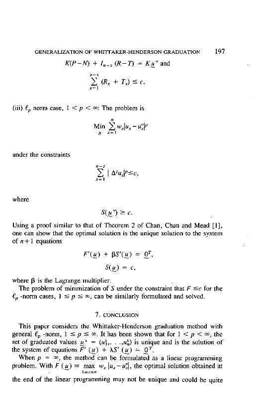
(iii) ep-norm case, 1 < p < ~: The problem is

Min ~ w x l u x - u " ~ ° u x = l


n- -z

Z l azux °<-c, X = I

where

S ( u " ) - c.

Using a proof similar to that of Theorem 2 of Chan, Chan and Mead [1], one can show that the optimal solution is the unique solution to the system of n + 1 equations

F ' ( u ) + 13S'(u) = 0 T,

S ( u ) = c,

where 13 is the Lagrange multiplier. The problem of minimization of S under the constraint that F -<c for the

~p -norm cases, 1 <- p -< ~, can be similarly formulated and solved.

7. CONCLUSION

This paper considers the Whittaker-Henderson graduation method with general ep -norm, ! -< p -< oo. It has been shown that for 1 < p < 0% the set of graduated values u x = (u~ . . . . . u~) is unique and is the solution of the system of equations F ' (u ) + hS' ( u ) = O r.

When p = 0% the method can be formulated as a linear programming problem. With F ( u ) = max w x lux-Uxl, the optimal solution obtained at

1 ~ x ~ n

the end of the linear programming may not be unique and could be quite

1 9 8 G E N E R A L I Z A T I O N O F W H I T T A K E R - H E N D E R S O N G R A D U A T I O N

far from the ungraduated values u " . The fit can be improved through quadratic programming. However , with F ( u ) = maxlu X - U"xl, no quadratic

I ~x~n programming is required.

For 1 -< p < ~, it is shown that F ( u ~) + hS (u~), F (uh ) , and S ( u ~) are, respectively, nondecreasing, nondecreasing and nonincreasing functions of k, and that there does not exist a u such that F ( u ) <- F ( u ~) and S (u ) -< S ( u ~) with at least one inequality being strict.

When 1 -< p -< ~ , it is shown that the alternative of minimizing F (or S) subject to S ~ c (or F <-- c) has some of its properties and solution algorithms analogous to the traditional method of minimizing F + hS.

APPENDIX l(a)

Here, 1 < p < oo. Let G: R --* R w i t h G ( y ) = lYe- Then

G'(y) = p sgn(y)lyt p- l

for every y and p, and

G"(y) = p ( p - l)lyp ' - z

except when y = 0 and p < 2 [3, p . 2 6 ] . For a func t ion M: R r ----~R s, define

p_Ml OM, q

°- . . . . . .

If

'mll "" " mlr l M = . . . . . . . . . . . . . . . ,

L m s , - • • m , , J

define M(y_) =-- M y with y ~ R r. Then M'(y) = M. If A: Rr ---~ R ~ and B: R s ~ R t, and B(A) is the composite function: Rr--* R', then the

Chain Rule is

where

C'()~) = B'(A(y)).A'(y),

C(Z) = B(A(y)).

Proof of Lemma 2.1 :

(i) F(u) can be expressed as B(A(u)), where

Then

GENERALIZATION OF WHITTAKER-HENDERSON GRADUATION

a ( u ) = , B(y) = ~ w~y~. x = l

fll'~ - u';p'- 'sgn(u, - u';) 0 ,,1

" 1

A ' ( u ) = 0 "'" pJu,, - u"F ° - Isgn(u,, - uT,)] ] '

199

B ' ( y ) = (w I . . . . . w,,).

So, by the Chain Rule,

F ' ( u ) = B ' ( A ( u ) ) A ' ( - u ) t t - - 1 t t = lpl,,,--u';V'-Csg.(u,-,,i') . . . . . p l , , . - . 2 ' sg,,( , ,°-u.)lw.

S(u) can be expressed as B(K(u) ) , where K is the ( n - z ) x n zth differencing matrix I I - - g

and B(y) = ~-'. [Yx~ with y ~ R"-:. Then K' (u) = K and B' (y) = [19 (sgn (y,))[y,[P-~, X = I

. . . . p (sgn Cv,,_z))]y,,_z[ p -1]. So, by the Chain Rule, S ' (u) = [ p [ A Z u ~ - ' s g n (AZu~),

. . . . plA Zu._ z[p - l sgn ( A Zu._ z) ]K.

(ii) The matrix ( F ' ( u ) ) r can be expressed as p ( W ( A ) ) ( u ) , where

a u, F ul sgn(u,, u,,)..J

L u - u "F~- , . _ ,,

Then, by the Chain Rule,

where

F"(u) = p ( p - I)WA'(u) = p ( p - I)A'(u)W,

0] A'(~) = u , - p~-?. lu.-u=V ~-2

The expression for S " ( u ) can he similarly derived.

P r o o f o f L e m m a 2 .2 :

For 1 < p < oo, G'(x) = p sgn~x~'- l is increasing. So G(x) = [x[p is strictly convex; for example, if x* 4: x, then for 0 < 0 < 1

2 0 0 GENERALIZATION OF WHI'I~I'AKER-HENDERSON GRADUATION

Iox* + (l-o)xl , ' < o~*lp + (1-o)~lp.

Therefore, if u ° 4: ~ , then for 0 < 0 < 1,

F(Ou* + ( l - 0 ) u ) = ~wxlOu* + ( l - 0 ) u x - u ~

= ~wxlO(u*~-u') + ( l -O)(u~-u")~ i = l

n n

ft < o Zw~lu~-u~ + (l-O) Zwxl,~-,~P i = l i - I

= F ( u * ) + ( 1 - 0 ) F ( u ) ,

that is, F is strictly convex. Furthermore, S is convex since S" is nonnegative definite.

Consequently, F + kS is strictly convex.

APPENDIX l(b)

The following APL program for carrying out the iterations in Theorem 2.2 is illustrated

by the numerical example (with p = 5, z = 3, h = 6) in Section 5.

VGRADI[-]]V V GRAD IV

[1] CRy--1 [2] -'-'~0 X tO = CR [3] FF~--P × ( w + . x ( × IV - u v ) × (llV

- U V ) * P - 1) + L × (~K) + . × ( × K + . × IV) × ([K + . × I V ) * P - 1 [4] A~--19 19 p, (~ ( I I V - U V ) *P- 2 ) , 19, 19 p0 [5] B~--J0,(~(IK+. x l V ) * P - 2 ) , J 0 0 [6] FFF~---P × ( P - I ) × ( W + . × A ) + ( L × ( O K ) + . × B + . × K) [7] D~---(BFFF) + . x FF [8] GV~--IV~--IV + 0.1 × UV = IVy---IV - D [9] F~--- + / W + . × (llV - U V ) * P

[101 S,---+/(IK+. ×IV)*P [11] M ( - - F + L × S [12] CR,- - (F / ID) ->0 .00001

[13] ---)2 V P~"-5 L~--6 J~---16 16 UV'~--34 24 31 40 30 49 48 48 67 58 67 75 76 76 102 101 100 115 134


IV*--36 22 33 38 32 47 50 46 69 56 69 73 78 74 104 98 103 113 136 K~---16 190-1 3 3 1 0 0 0 0 0 0 0 0 0 0 0 0 0 0 0 0 W~--19 190, (19 103 5 8 10 15 20 23 20 15 13 II 10 9 9 7 5 5 3 l), 19 1900

GRAD IV

GV 29.92 43.26 66.94 94.49 128.25 F 1148648 S 20156 F + L x S 1329589

28.72 31.22 33.99 36.50 48.54 53.70 60.60 63.58 69.83 73.74 83.03 101.93 107.01 114.56

Explanation of Symbols

P = NORM L = LAMBDA UV = UNGRADUATED VALUES IV = INITIAL ITERATION VALUES K = ZTH DIFFERENCE MATRIX

W = WEIGHT MATRIX GV = GRADUATED VALUES F = FIT S = SMOOTHNESS

APPENDIX I1

Proof of Theorem 3.1: The (LP) problem has at least one feasible solution if f and s are large enough.

Furthermore, an optimal solution to (LP) always exists because the objective function, which is to be minimized, is bounded below [9, p.97].

If (u ~, f~, sx) is an optimal solution to (LP), then by (3. la) and (3. Ib)

F ( u ~) < f~ and S(u ~) <-- s~.

Suppose that one of the above inequalities, say the first inequality, is a strict inequality. Then F ( u x) + h S ( u O < f~ + hs~. Since

F ( u ~) = max wxlu x - u~" I >-- wxlu x - u~l for x = 1 . . . . . n,

(3.1a) is satisfied with f = F(u~). This is contradictory to ( u ~, f~, s~) being optimal. So

202 GENERALIZATION OF WHIT'FAKER-HENDERSON GRADUATION

f~ = F ( u ~) and s~ = S(u~).

If Uo is an optimal solution to (WH), that is,

fo +kSo = Min[F(u) + kS(u)], u - 0

wherefo ------ F( u °) and s o =-- S( u°) , then

wxlu ° - u~] ~fo for x = 1 . . . . . n,

I Azu°[ <- So f o r x = 1 . . . . . n--z ,

and, hence, u o satisfies the constraints (3. l a) and (3.1b) of (LP). Since (u h, f~, s~) is an optimal s~ution to (LP),

f~ + ash <--fo + hSo.

But the minimization in (WH) is over all u,

f~ + hs~ >- fo + hSo.

Therefore

L + hs~ = f o + kSo,

and u h is an optimal solution to (WH).

APPENDIX IIl

Proof of Theorem 4.1: If h > h* --> 0, then

F ( u x*) + X*S(u ~*) -< F ( u ~) + k*S(u ~) -<F(u ~) + kS(uX). (1II.1)

The second inequality is strict if S (u ~) > 0 and, hence, the first Monotone Property holds.

By adding the first inequality in (IlL I) to the similar inequality

F (u" ) + hS(u ~) ---< F ( u x*) + hS(u~*),

we obtain

0 -< ( x - x*) [S(u ~*) - S(u~)].

That is, S (u ~) -< S (uh*). This and (III.1) imply that F ( u ~*) -< F(u~). Now we proceed to show that for 1 < p < 0% S(u ~) < S(u ~*) if S(u ~) > 0. This

holds if the first inequality in (11I. 1) is strict. If this is not true, then

F ( u ~*) + h*S(u x*) = F ( u ~) + h*S(u~'),

and u ~* ¢ u ~, implying that the optimal solution to (WH) is not unique. This contradicts


Theorem 2.1. Consider the fact that u ~* ~ u x comes from F' (u ~) + hS'(u)) = ~0 = F'(u ~*) + h*S'(u ~*) (see Theorem 2.1) and the assumption that S(u~)>0. Suppose u x~'= uh; then we have h*S'(u ~*) = hS'(u~), which implies that S '(u ~) -- S ' (u ~*) = 0. Since

S ' (u ~) = p[lAZu~-~sgn(/XZu~) . . . . . IZ~u~_~l p - ~ sgn(A"u~_z)]g ,

S ' (u x) = Oimplies that I/VUx~ = 0 fo ra l l 1 -<x--< n - z ; t h a t is, S(u~) = 0_ which contradicts the assumption.

The first inequality in (III. 1) and S(uX)<S(u *) implies that F(u~)>F(u'*). To see that (F(u~), S(u~)) is Pareto-optimal, suppose that u is such that F(u) <

F(u~), and that S(u) -< S(u~); then

F(u) + k S ( u ) < F(u ~) + hS(u~),

which contradicts the assertion that u x minimizes F(u) + hS(u).

REFERENCES

1. CHAN, F.Y., CHAN, L.K., AND MEAD, E.R. "Properties and Modifications of Whit- taker-Henderson Graduation," Scandinavian Actuarial Journal, 1982, 57-61.

2. CHAN, F.Y., CHAN, L.K., AND MEAD, E.R. Discussion on "An Extension of the Whittaker-Henderson Method of Graduation," TSA, XXXIV (1982), 368-369.

3. FLEMMING, W.H. Functions of Several Variables, Reading, MA: Addison-Wesley, 1965.

4. GERBER. H.U. An Introduction to Mathematical Risk Theory, Homewood, IL: Irwin, 1980.

5. GREVILLE, T.N.E. "Part 5 Study Notes---Graduation," Chicago, IL: Society of Actuaries, 1974.

6. GREVILLE, T.N.E. Discussion on "A Linear Programming Approach to Gradua- tion," TSA, XXX (1978), 442.

7. HICKMAN, J.C., AND MILLER, R.B. "Notes on Bayesian Graduation," TSA, XXIX (1977), 7-21.

8. HICKMAN, J.C., AND MILLER, R.B. "Bayesian Bivariate Graduation and Forecast- ing," Scandinavian Actuarial Journal, 1981, 129-150.

9. HILLIER, F., AND LIEBERMAN, G. lntroduction to Operations Research (3rd Edition), San Francisco, CA: Holden-Day, 1980.

10. HOFFMAN, K. Analysis in Euclidean Space, Englewood Cliffs, NJ: Prentice-Hall, Inc., 1975.

1 I. LOWRIE, W.B. "An Extension of the Whittaker-Henderson Method of Graduation," TSA XXX1V (1982), 329-72.

12. MORDECAi, A. Nonlinear Programming, Englewood Cliffs, N.J.: Prentice-Hall, lnc., 1976.

204 GENERALIZATION OF WHITTAKER-HENDERSON GRADUATION

13. MILLER, M.D. Elements of Graduation, New York, NY: Actuarial Society of Amer- ican and American Institute of Actuaries, 1946.

14. SCHUEa~rE, D.R. "A Linear Programming Approach to Graduation," TSA, XXX (1978), 407--445.

15. SHIU, E.S.W. "Matrix Whittaker-Henderson Graduation Formula," ARCH, Chi- cago, IL: Society of Actuaries, (1977), Issue No. I.

16. WHWrAKER, E.T., AND ROBINSON, G., The Calculus of Observations, London: Blackie and Son, Ltd., 1924.

DISCUSSION OF PRECEDING PAPER

ELIAS S. W. SHIU:

This paper is an interesting extension of Schuette [7]. The results here can be generalized to the case where F and S are formulated by different ~p-norms. The p for F should be small to diminish the effects of the outliers. The p for S should be large so that the graduated sequence is uniformly smooth. Thus, the problem is to minimize

wxlux - uxl + h maxlA z Uy[. x y

For elaboration on the above, see [7], pages 434-45. Indeed, the concept of Whittaker-Henderson graduation can be further

generalized as: Find u which minimizes

h(u) = f ( u - u") + g (Ku) ,

where f and g are convex functions. In the case where

f ( x ) = x r W x

and

g(x) = h x r x ,

we have the classical Whittaker-Henderson type-B graduation. Let us assume that the convex functions f and g are twice-differentiable. Then, it may be possible to solve the equation

h ' (u ) = O r

by Newton-Raphson iterations

uk+l = u k _ [h" (Uk)]-l [h,(uk)]r,

where

and

h ' (u ) = f ' ( u - u " ) + g ' ( K u ) K

h"(u) = f ' ( u - u") + l ( rg" (Ku)K.

Note that the matrix K need not be a differencing matrix; see Greville [3], page 389.

205


In formulating the minimization problem, one should also specify the constraints

0 _ < u x _ < 1,

if the ux's are probabilities. Furthermore, linear constraints such as

c(x)u x + d(x) <- ux ÷ 1

may be imposed on the graduated values as desired. The problem becomes one o f minimizing

h(u) , ueC , (1)

where C is a closed and convex subset o f R n. For a differentiable function h, a vector r e C satisfies

h(r) = Min h(u) (2) u~C

only if

h ' ( r ) (u - r) >- 0 for e a c h u e C . (3)

In general, (3) does not imply (2) unless h is convex (or pseudo-convex). Since minimizing a nonlinear function of many variables under constraints

is computationally complex, how does one minimize (1)? A solution has been forwarded eloquently by W. Conley [2]:

Computer technology has advanced to the point that it is now possible to take an entirely different philosophical approach to the statement and the solution of mathematical optimization problems. In the past, each optimization problem had to be stated in the form of a standard model, for example, in a linear problem whether or not this was an accurate reflection of reality. This was necessary because only these standard models had theoretical solution procedures. If these procedures were followed, then a small amount of calculation produced the result. However, computers have become so fast and computer time so accessible and inexpensive that it is now possible to state any optimization problem (linear or nonlinear) as a completely accurate reflection of reality and let the computer search all the possible solutions (or a large sample of solutions) and produce the optimum regardless of the functional form of the problem.

Goodness o f fit is often considered in conjunction with chi-square testing. Taylor [8] shows that it is not correct to use the chi-square test to test the goodness o f fit o f a linear compound graduation, and the Whittaker-Hen- derson method is a linear compound graduation. However, some recent literature (such as [1] and [5]) does not consider this result. For further discussion, see [4].

The multivariate calculus is a useful tool in many developments. Below are two examples.

DISCUSSION 207

(i) Assuming differentiability, one may rephrase the first part of Theorem 4.1 as

d - ~ [F(u(h)) + LS(u(h))] --> 0, (4)

where u(h) = uh satisfies the equation

F'(u()Q) + S'(u(X)) = 0 7".

By the Chain Rule and the Product Rule,

d [F(u(X)) + XS(u(X))]

= F'(u(h))u ' (h) + XS'(u(h))u'(h) + S(u(h))

(5)

= O r u ' ( X ) + S(u(h)) -.'(5)

= S(u(X)).

Thus we have (4).

(ii) The problem considered in [6] is the minimization of the quadratic form

q(u) = ( u - u " ) r W ( u - u " ) + ( u - s ) r V ( u - s ) + (Ku) r (Ku),

where W and V are diagonal matrices. The minimum vector u is the solution to the equation

q'(u) = O r.

Since

q'(u) = 2 [ ( u - u " ) r W + ( u - s ) r V + urKrK],

the result of [6] follows.

REFERENCES

1. BENJAMIN, B., AND POLLARD, J. H. The Analysis of Mortality and Other Actuarial Statistics, London: Heinemann, 1980.

2. CONLEY, W. Computer Optimization Techniques, Princeton: Petrocelli Books, 1980. 3. GREVILLE, T. N. E. "A Fortran Program for Generalized Whittaker-Henderson Grad-

uation," ARCH, 1982.1, Chicago: Society of Actuaries, 385-401. 4. HOEM, J. M. "A Contribution to the Statistical Theory of Linear Graduation," In-

surance: Mathematics and Economics, II1 (1984), 1-17. 5. LONDON, R. L. Graduation: The Revision of Estimates, Part 5 Study Note 54-01-

84, Itasca: Society of Actuaries, 1984. 6. LOWRIE, W. B. "An Extension of the Whittaker-Henderson Method of Graduation,"

TSA, XXXIV (1982), 329-50; Discussion 351-72.


7. SCHUETTE, D. R. "A Linear Programming Approach to Graduation," TSA, XXX (1978), 407-31 ; Discussion 433-45.

8. TAYLOR, G. C. "The Chi-Square Test of a Graduation by Linear-Compound For- mula," Bulletin de l'Association Royale des Actuaires Belges, LXXI (1976), 26-42.

E.S. ROSENBLOOM:*

This paper presents algorithms for performing the Whittaker-Henderson graduation method of mihimizing F ( u + S(u) over all u = (ui, u2 . . . . . u,) r . In section 2, the authors use the ep-norm with 1 < p < oo to obtain the following nonlinear minimization problem:

Min [F(u) + k S (u)] u

where

and

= x = l

n--Z

s ( s ) = I Vzu ' x = l

i i t t (h, p , w l, w 2 . . . . . Wn, u l , u2, are fixed constants).

The Newton-Raphson iterative technique is the algorithm used to find the optimal solution to this problem. In this algorithm, a sequence of vectors u k is generated using the recurrence relationship

.UR k + l = ~.R k -- [ F " ( u k) -k- ~. S" (..uRk)] - I [ F t ( u k) @ h S' (URk)] T. (1)

The strict convexity of the objective function ensures that if {u k} converges to u , then u will be the unique optimal solution to the nonlinear program.

The Newton-Raphson algorithm is one of the oldest numerical techniques available for minimizing nonlinear functions. It has the advantage that when it converges, it converges at a quadratic rate. However, the Newton-Raphson method is rarely used today to solve nonlinear problems because it has certain drawbacks.

Formula (1) does not ensure a decrease in the function value at each iteration. In other words, it is possible that

F ( u k+t) + h S ( u k+l) > F ( u k) + h S ( u k ) .

To remedy this situation the modified Newton-Raphson formula is often used:

*Dr. Rosenbloom, not a member of the Society, is an Assistant Professor with the Department of Actuarial and Management Sciences, University of Manitoba.

u k+~ = u k - 0 k [ F ' ( u k) +

where 0 k is a scalar chosen so

F (U k+l) "Jr- h S

In one variation, O k is chosen 0 d k) with respect to 0 where

DISCUSSION 209

h S" (uk)] -1 [F' ( u k) + h S' (uk)] r (2)

that

( u k+l) < F ( u k) + h S ( u k ) .

to minimize F ( u k + 0 d k) + h S ( u k + d k is the search direction

- [F" ( u k) + h S" (uk)] - ~ [F' ( u k) + X S' (uk)] r.

Another drawback of the Newton-Raphson method is that even with the assumption of strict convexity of the objective function F (u ) + h S (u) , the Hessian matrix F" ( u k) + h S" ( u k) may be singular. In that case, formula (1) would be undefined.

For large values of n, the most serious drawback of the Newton-Raphson method is the enormous amount of computation required at each iteration. Even exploiting the fact that the Hessian matrix F" ( u k) + h S" ( u k) is symmetric, formula (1) requires computing n 2 + n second partial derivatives and 2n first partial derivatives. In addition, a system of equations needs to be solved in order to obtain the search direction d k.

To avoid the drawbacks of the Newton-Raphson method a number of techniques have been developed over the last twenty-five years. The most popular of these techniques are the Quasi-Newton methods. The Quasi- Newton methods generate a sequence of vectors {u k} by a recurrence relationship of the form.

u k+~ = u k - 0 k H k [ F ' ( u k) + X S ' ( u k ) ] r . (3)

H k is an n x n matrix which may approximate the inverse Hessian matrix IF" ( u k) + h S" ( u k) ] - l . 0 k is chosen to minimize F ( u k + 0 d k) + h S ( u k + 0 d k) with respect to 0 with d k being the direction - H k [ F ' ( u k) + X S' ( u k) ]r.

In general, the Quasi-Newton methods require considerably less computation than the Newton-Raphson methods. They do not require the computation of second partial derivatives. In addition, they tend to be more robust than the Newton-Raphson methods.

The various Quasi-Newton methods differ in how the matrix H k is obtained. Numerical experiments have indicated that the most successful of the Quasi-Newton methods is the Broyden-Fletcher-Goldfarb-Shanno algorithm. In this algorithm, the matrix H k is obtained using the formula

(l +(qk)r Hk qk) Pk (Pk) r nk+l = Hk + (qk)r pk ~ k ) r q k

pk (qk)r Hk + H k qk (pk)T . . . . . (4) (qqk)r p k


where

H ° is any positive definite matrix,

p k = u k _ u ~ - l , and

qk = [ F ' ( u k) + X S' ( u k) ] r _ [ F ' ( u k-I) + h S' ( u k- l ) ]7-.

A more complete discussion of Quasi-Newton methods and other alter- natives to Newton-Raphson can be found in [4] or [5].

REFERENCES

1. AVRIEL, M. Nonlinear Programming, Englewood Cliffs: Prentice Hall, 1976. 2. FLETCHER, R. "A New Approach to Variable Metric Algorithms," Computer Journal

13 (1970), 317-22. 3. GmL, P.E., AND MtJRRAV, W. "Quasi-Newton Methods for Unconstrained Optim-

ization," Journal of the Institute of Mathematics and ITS Applications 9 (1972), 91- 108.

4. GmL, P.E., MURRAY, W., AND WRIGHT, M.H. Practical Optimization, New York: Academic Press, 1981.

5. LUENBERGER, D.G. Linear and Non-linear Programming, Reading, Mass.: Addison- Wesley, 1984.

6. MURR?,V, W. Numerical Methods for Unconstrained Optimization, New York: Ac- ademic Press, 1972.

(AUTHORS' REVIEW OF DISCUSSION)

FUNG YEE CHAN, LAI K. CHAN, AND MAN HEI YU:

Dr. Shiu generalizes F + kS using a formulation which covers a wide range of cases. Multivariate calculus can then be applied to the graduated values u k and used to derive the monotone properties.

The problem of minimizing

wxlux-ux"l ÷ XmaxlAZUyl x y

and other related problems, of which the norms of F and S are different and are e l , 22 or e®, have been investigated by us in a separate study.

We agree with Dr. Shiu's comment that, due to the advances of computer technology, new approaches in the formulation and solution procedures for the Whittaker-Henderson graduation should be explored. Recently, we have been working on a statistical data analysis approach of selecting h.

Dr. Rosenbloom gives a comprehensive description of contemporary techniques which improve the traditional Newton-Raphson method.

In his 1974 Part 5 Society of Actuaries Study Note on graduation, Dr. Thomas Greville elegantly used linear algebra to formulate and solve the

DISCUSSION 211

Whittaker-Henderson graduation problem. His work has inspired using mod- em mathematics in research work on graduation. This paper and the two discussions represent some of the inspiration.

We would like to take this opportunity to thank Dr. Greville, who has contributed so much to the development of graduation methodology.

Documents

A Generalization of Whittaker-Henderson Graduation - Society of