NetnomicsDOI 10.1007/s11066-008-9022-1

A game theory modeling approach for 3G operators

Dimitris Katsianis · Attila Gyürke ·Rozália Konkoly · Dimitris Varoutas ·Thomas Sphicopoulos

Accepted: 18 August 2008© Springer Science + Business Media, LLC 2008

Abstract This paper presents the technoeconomic evaluation of a third gener-ation rollout scenario followed by the identification of the market conditionsfor two operators in a simple game theory model. The considered scenariosreflect the point of view of both dominant operators and new entrants. Tech-noeconomic results are presented in terms of net present value (NPV), actinglike the pay-off function in the proposed theoretical Game Theory model.The business case presented here was studied by using a tool, developed byEuropean Projects IST-25172 TONIC/ECOSYS, a model developed by theEURESCOM P901 project and the Game Theory Tool named Gambit.

Keywords Technoeconomics · Techno-economics · Game theory · NPV ·Investment UMTS · 3G · Market conditions · Telecommunications

1 Introduction

The investigation of a 3G rollout investment case (UMTS) is one of the hottopics in the last decade for the telecommunication operators and investors.This is true in both technical and economical points of view. In fact, these allpertain to global liberalization of Telecommunication and to the competition

D. Katsianis (B) · D. Varoutas · T. SphicopoulosDepartment of Informatics and Telecommunications,University of Athens, Athens, Greecee-mail: dkats@di.uoa.gr

A. Gyürke · R. KonkolyMagyar Telekom, Budapest, Hungary

D. Katsianis et al.

raise when the operators purchase the licenses. So, one of the main viewpointshere should be necessarily the competition and its impacts on business, throughtechnoeconomic (TE) analysis.

Technoeconomic analysis of telecommunication systems and services, com-bining the economical and business aspects with comprehensive technicalparameters, has attracted the interest of many researchers worldwidely andseveral studies have been published, especially during the last decades aimingto offer quantitative and qualitative answers to questions about the telecomtechnology and business strategy [1–5]. However, especially towards the quan-titative modeling, the business modeling as well as the business or making-profit strategies has to be combined with market forecasts, willingness-to-paydata, and cost modeling of both operational and capital expenditures in a rightcombination in order to produce balanced and therefore reliable results.

In order to incorporate competition analysis in every technoeconomicanalysis, of a game theory provides a solid mathematical methodology for suchpurposes although the combination of game theory approach with traditionaldiscount cash flow (DCF) analysis has not been widely published. Most of thearticles available in the literature are based on the traditional DCF combinedonly with sensitivity and risk analysis, aiming to include uncertainty modeling.On the other hand, game theory has been widely used in telecommunicationsin radio resource management problems [6–10]. In [11], a general methodologyto quantify the option value in technology investments based on option andgame theory is proposed with possible application to capacity expansionproblems of telecommunications, but without any specific application andnumerical results. In conclusion, to the best knowledge of the authors, there isno complete analysis of any telecommunications investment case using gametheory on top of traditional DCF analysis.

In this paper a simple UMTS investment case model following a gametheory approach is presented, which was based upon near real business condi-tions and figures. This model could be easily expanded and used with modifiedmarket conditions and tariff schemes. The rest of the paper is organized asfollows. In Section 2, the methodology used is presented while in Section 3, theparameters and the assumptions of the technoeconomic modeling along withthe necessary mathematical background are described. Section 4 summarisesthe results of the modeling and finally Section 5 concludes the analysis andintroduces future topics.

2 Methodology

The case presented within this article offers numerical results aiming toquantify the 3G competition problem. This investment analysis was carriedusing the tool, which was developed by IST TONIC [12–14], and the ECOSYSproject [15] and a game theory model developed by EURESCOM (EuropeanInstitute for Research and Strategic Studies in Telecommunications GmbH)

A game theory modeling approach for 3G operators

P901 project [16]. A 10-year time frame, spanning the period 2004 to 2014has been chosen. In order to calculate discounted cash flows, a discountrate of 10% has been selected. Tariffs, market penetration of both fixedbroadband and mobile services in various European countries and existingforecasts for UMTS services were gathered, and an analytical market modelwas developed [2]. The main assumptions regarding tariff policy as well asmarket conditions are analytically described in [2]. The area study representsa central or southern European country with higher population density (60million) and lower mobile penetration (40%). The areas are composed ofdense downtown zones surrounded by less dense peripheral zones, and largersuburban areas The UMTS network is assumed to cover 80% of the totalpopulation and total mobile penetration is assumed to saturate at 80% (phoneowners, not number of terminals) in 2009. Service classes are described in [2]and [3] as well as analytical TE results for the regular financial analysis.

2.1 Structure of the tool for technoeconomic evaluation

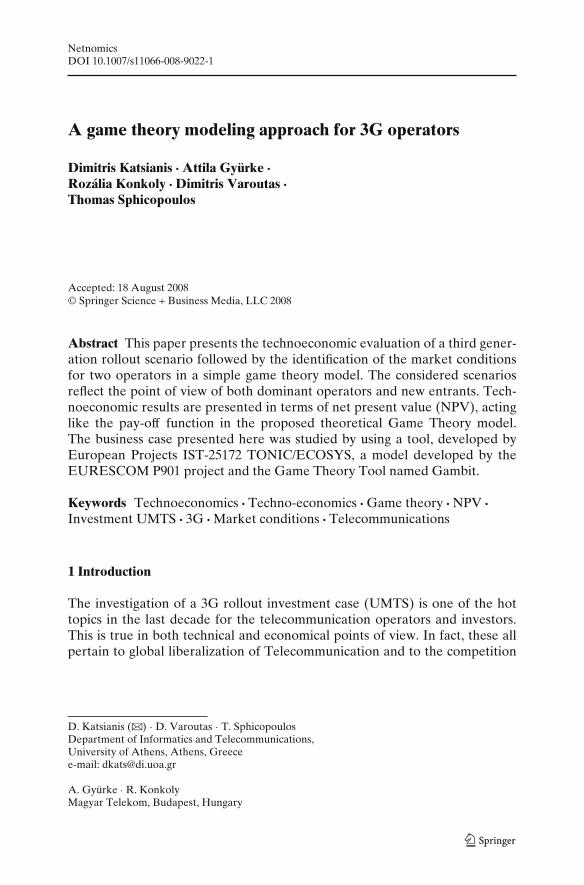
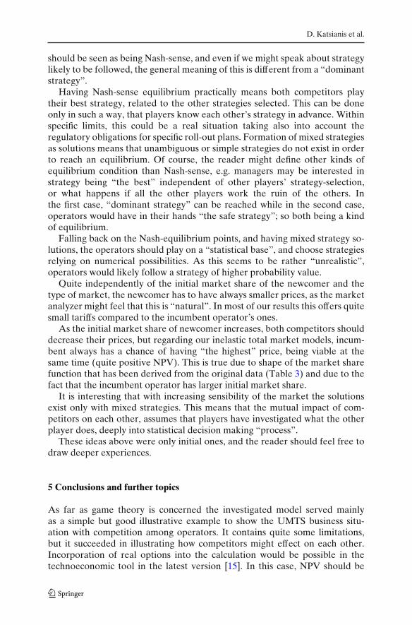
Figure 1 analyses the main principles of the methodology used in this paper.The cost figures for the network components have been collected in anintegrated cost database, which is the “heart” of the model. This databaseis frequently updated with data obtained from the major telecommunicationoperators, suppliers, standardization bodies and other available sources. Thesedata correspond to the initial prices for the future commercial network com-ponents as well as to the projection for the future production volume of them.The cost evolution of the different components derives from the cost at a given

Volume Class

OA&M Class

Cost Evolution

ComponentsDatabase

Operators

Suppliers

Standardizationbody

Other

Size

Policy

MarketSize

Tariffs

Policy

User inputs

Operators

Surveys

Decision Index

calculation(NPV, IRR,

Payback period)

Finan

cial M

odel

Year n

. . .Year 2

Revenues

Cash Flows

Profits

Investments

Year 1

Radio ModelArchitectures

Services

Real OptionsGame

Theory

Fig. 1 Technoeconomics methodology and the connections with the game theory and real optionsmodeling [2]

D. Katsianis et al.

reference year and a set of parameters, which characterizes the basic principlesof the component. For each component in the database, the cost evolutionis estimated according to a cost evolution model [1] and [17]. In addition,estimations for the operation administration and maintenance cost as well asthe production volume of the component are incorporated in the database.As a next step in the network evaluation, the services to be provided to theconsumers should be specified. The network architectures for the selectedset of services will be defined, and a radio model, has been used in order tocalculate base transceiver station positions as well as the civil works for theirinstallation (database data). The future market penetration of these servicesand the tariffs associated, according to each operator’s policy, will be usedfor the construction of the market evolution model. The operator tariff policycould be taken into account by modifying the tariff level in conjunction withthe expected penetration of the offered services. Results from statistics orsurveys can be easily integrated into the tool when formulas measuring theimpact of tariff level to the saturation of the services are available.

By entering the data into a financial model we calculate the revenues, invest-ments (and IFC) cash flows and profits (or other financial results) of the studiednetwork architectures for each year throughout a project’s study period. In thefinal evaluation of the technoeconomic model, critical indexes are calculatedin order to decide about the profitability of the investment. The methodologyis illustrated in Fig. 1. The adoption of alternative financial and strategicmethods, e.g. real options approach and game theory, can be included inthe tool.

2.2 Game theory modeling

To keep simplicity, the initial technoeconomic model described in [2] hasbeen used. The new model [16] has been build, based on the following mainassumptions:

1. We investigated an Oligopoly, or more precisely Duopoly case. As it wasconsidered to be realistic (in terms of modeling) the number of playerswould be only two, and one of them would be the incumbent operatorwith high market share, whereas the other would be a new company withrelatively small market share and with Greenfield investment needs.

2. For not being complicated we decided to see the market for UMTS servicesas a homogenous market with only one product. It means we “merged” allservices and market segments to one, independently of different frequen-cies used and tariffs applied.

3. During calculation we have not taken into account the feedback thatgeneral price levels have on the total market, so the total market was stableor insensitive. We supposed transmigration (churn effects) only betweencompetitors, which means dynamic market inside.

4. The game was built as being a non-cooperative game, which means bothplayers know everything of importance about the other, but they make

A game theory modeling approach for 3G operators

decisions approximately at the same time and independently. In this caseplayers are not allowed to form any kind of coalition.

5. At this stage of the work we “voted” to keep the game static with onlyone decision point at the beginning of the estimated time period (in caseof longer time horizon this could fail to be “realistic”). This one decisionpoint might be e.g. just before the national auctions or beauty contest forfrequency allocation.

6. In this UMTS example companies play price-adjusting game and quantities(quantity here refers to the size and costs of investment for network andinfrastructure) do not produce an effect on the results considerably (thisseems to be realistic, as a simple investment in the global coverage mightbe sufficient through the investigated period).

7. The pay-off function of the game was decided to be the NPV of a 10-yearslong investment period, and in the first step we let out the calculations withreal options values [18], so skipping the “adjusted” NPV that could havebeen produced.

3 Technoeconomic modeling

The calculations were based on two main inputs from the TE model resultsand the hypothetical (empirical) market parameters. The TE model served asthe main root for calculating inputs of our calculations. So we accepted all thesuppositions built into the TE model, and different models for “incumbent”and “newcomer” were prepared. We followed the 10-year time horizon, andnaturally all the investments, costs and revenue figures. All the other basicparameters were set to illustrate an “average western European case”.

To be able to calculate the pay-off, two important parameters were pickedup, namely:

◦ The market share and◦ The tariff multiplier or in other words the “price”

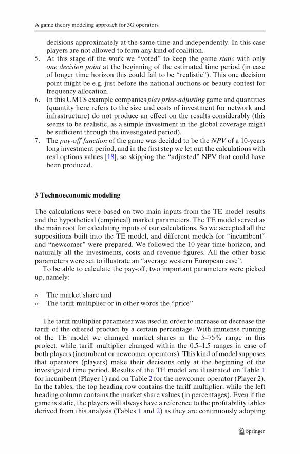
The tariff multiplier parameter was used in order to increase or decrease thetariff of the offered product by a certain percentage. With immense runningof the TE model we changed market shares in the 5–75% range in thisproject, while tariff multiplier changed within the 0.5–1.5 ranges in case ofboth players (incumbent or newcomer operators). This kind of model supposesthat operators (players) make their decisions only at the beginning of theinvestigated time period. Results of the TE model are illustrated on Table 1for incumbent (Player 1) and on Table 2 for the newcomer operator (Player 2).In the tables, the top heading row contains the tariff multiplier, while the leftheading column contains the market share values (in percentages). Even if thegame is static, the players will always have a reference to the profitability tablesderived from this analysis (Tables 1 and 2) as they are continuously adopting

D. Katsianis et al.

Tab

le1

Ope

rato

r1-p

laye

r1

(inc

umbe

nt)

NP

Vs

inBe

Mar

ket

Tar

iffm

ulti

plie

rsh

are

(%)

0.5

0.6

0.7

0.8

0.9

11.

11.

21.

31.

41.

5(−

50%

)(−

40%

)(−

30%

)(−

20%

)(−

10%

)(+

10%

)(+

20%

)(+

30%

)(+

40%

)(+

50%

)

51.

692.

393.

123.

814.

515.

205.

896.

587.

287.

978.

6610

2.38

3.18

3.99

4.77

5.55

6.33

7.12

7.90

8.68

9.46

10.2

415

3.08

3.96

4.86

5.73

6.60

7.47

8.34

9.21

10.0

810

.95

11.8

120

3.77

4.74

5.73

6.69

7.65

8.61

9.56

10.5

211

.48

12.4

413

.39

254.

465.

526.

607.

648.

699.

7410

.79

11.8

412

.89

13.9

314

.97

305.

166.

317.

478.

609.

7410

.88

12.0

113

.15

14.2

915

.42

16.5

535

5.85

7.11

8.34

9.56

10.7

912

.01

13.2

414

.47

15.6

916

.91

18.1

340

6.54

7.89

9.21

10.5

211

.84

13.1

514

.47

15.7

817

.10

18.4

019

.71

457.

248.

6710

.08

11.4

812

.89

14.2

915

.70

17.1

018

.50

19.9

021

.30

507.

939.

4510

.95

12.4

413

.94

15.4

316

.92

18.4

219

.91

21.3

922

.88

558.

6310

.24

11.8

213

.40

14.9

916

.57

18.1

519

.74

21.3

122

.89

24.4

660

9.32

11.0

212

.69

14.3

616

.04

17.7

119

.38

21.0

522

.72

24.3

826

.05

6510

.01

11.8

013

.56

15.3

217

.08

18.8

520

.61

22.3

724

.12

25.8

827

.63

7010

.71

12.5

814

.43

16.2

818

.13

19.9

821

.84

23.6

825

.53

27.3

729

.21

7511

.42

13.3

615

.30

17.2

419

.18

21.1

223

.06

25.0

026

.93

28.8

630

.80

A game theory modeling approach for 3G operators

Tab

le2

Ope

rato

r2-p

laye

r2

(new

com

er)

NP

Vs

inBe

Mar

ket

Tar

iffm

ulti

plie

rsh

are

(%)

0.5

0.6

0.7

0.8

0.9

11.

11.

21.

31.

41.

5(−

50%

)(−

40%

)(−

30%

)(−

20%

)(−

10%

)(+

10%

)(+

20%

)(+

30%

)(+

40%

)(+

50%

)

5−2

.32

−2.0

7−2

.00

−1.8

3−1

.18

−0.9

3−0

.69

−0.4

5−0

.20

0.04

0.28

10−1

.58

−1.2

4−1

.03

−0.7

5−0

.09

0.25

0.58

0.91

1.25

1.58

1.91

15−0

.84

−0.4

1−0

.07

0.33

1.00

1.43

1.85

2.27

2.69

3.12

3.54

20−0

.10

0.41

0.89

1.42

2.09

2.61

3.12

3.63

4.14

4.66

5.17

250.

631.

241.

852.

503.

193.

794.

394.

995.

596.

196.

8030

1.37

2.07

2.81

3.59

4.28

4.97

5.66

6.35

7.04

7.73

8.42

352.

112.

923.

804.

595.

376.

156.

937.

718.

499.

2710

.05

402.

843.

824.

725.

596.

467.

338.

209.

079.

9410

.81

11.6

745

3.64

4.67

5.63

6.59

7.55

8.51

9.47

10.4

311

.39

12.3

413

.29

504.

435.

496.

547.

598.

649.

6910

.74

11.7

812

.83

13.8

714

.92

555.

176.

317.

458.

599.

7310

.87

12.0

013

.14

14.2

715

.40

16.5

460

5.90

7.13

8.36

9.59

10.8

212

.04

13.2

714

.49

15.7

116

.94

18.1

665

6.63

7.95

9.27

10.5

911

.90

13.2

214

.53

15.8

517

.16

18.4

719

.78

707.

368.

7710

.18

11.5

912

.99

14.4

015

.80

17.2

018

.60

20.0

021

.40

758.

099.

5911

.09

12.5

914

.08

15.5

717

.06

18.5

520

.04

21.5

323

.02

D. Katsianis et al.

their prices to competition. So the profit margin could be always defined viathe numerical results from the sensitivity analysis (Tables 1 and 2).

3.1 Hypothetical–empirical market parameters

Only for emphasizing assumptions regarding the market, we supposed that thetotal market is stable, and only transmigration between competitors was takeninto account. This is combined with having only one “product,” which on onehand means that all services were merged to one, and on the other part thereis no additional real market segmentation except the segmentation describedin [2].

In the price-adjusting model, “price-war” was assumed, and we tried todepict this “war” by a hypothetical transmigration market function. The simplereason behind this is that when one of the players decreases his price relatedto the other’s, the cheaper operator will reach the higher portion of the marketshare, namely when lowering the price compared to the competitor’s, a gainmarket share will be obtained.

The difference between tariff multipliers (denoted by x) should be limitedby the interval defined for the tariff multipliers for the two operators (denotedby TM1 and TM2). So TM1 and TM2 should be chosen from the [0.5, 1.5]and the difference of the tariff multipliers (TM1–TM2) will be limited in the[−1, 1] interval. When x is 0, the tariffs are equal and when x < 0 thenPlayer 1 offers more competitive product (with lower price). In general forthe telecommunication market we are not able to collect data for the x valuesnear to −1 or 1 since operators usually are not able to sell products in tripleprice than the competitor’s. (In case of x = 1 or x = −1 there is a three timesdifference in the product prices regarding the players, i.e. one product 50 andthe other 150 euros).

There are a number of problems with the construction of the functionthat controls the market share of the operator. In our calculation the marketfunction and plots are built from the newcomer operator’s (player 2) point ofview. The definition of the market behavior function due to the price changes(from the point of view of player 2) follows some “logical” rules described asfollows:

1. Value domains [MSDMin, MSDMax] minimum and maximum variation ofthe market share (defined by the user each time)

2. The function applied in the value domain (MSDMax) should be limited inthe interval [0, 1] and −1 < x < 1, where x is the relation of the tariffs(which shows the increase or decrease of tariffs for the offered servicesregarding the two operators). This constraint relies on the fact that anoperator cannot lack more than 100% of its initial market share

3. Slope: for large values of x the function quickly reaches the saturationlevel, which means that the maximum market share cannot change further.

4. For x < 0 the function derives to 1 and actually to MSDMin in the finalimplementation.

A game theory modeling approach for 3G operators

Fig. 2 Shape of thehyperbolic tangent function

tanh(x)

-1,00-0,80-0,60-0,40-0,200,000,200,400,600,801,00

-1-0

,8 -0,6

-0,4

-0,2 0

0,2

0,4

0,6

0,8 1

tanh(x)

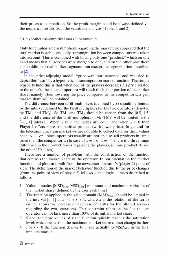
5. The slope should be steeper near zero, which means that the marker (sub-scribers) is sensitive with respect to small changes of tariffs. Furthermore,this slope depends on different market behaviours. Thus, it is desirable tobe able to adjust this slope. Different market reaction will be tested in theimplementation of the model.

Some example functions that could meet some of the above criteria are well-known and can be generated from the hyperbolic tangent function (tanh(x))

(or from the –x function when rule 4 is applied) and are defined by:

f (x) = ex − e−x

ex + e−x(1)

f (b x + a) = eb x+a − e−b x−a

eb x+a + e−b x−a(2)

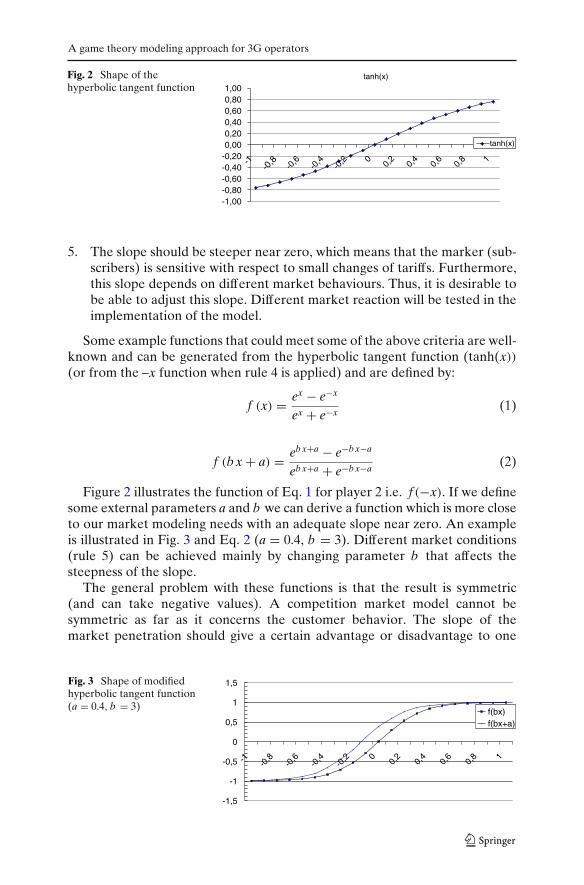
Figure 2 illustrates the function of Eq. 1 for player 2 i.e. f (−x). If we definesome external parameters a and b we can derive a function which is more closeto our market modeling needs with an adequate slope near zero. An exampleis illustrated in Fig. 3 and Eq. 2 (a = 0.4, b = 3). Different market conditions(rule 5) can be achieved mainly by changing parameter b that affects thesteepness of the slope.

The general problem with these functions is that the result is symmetric(and can take negative values). A competition market model cannot besymmetric as far as it concerns the customer behavior. The slope of themarket penetration should give a certain advantage or disadvantage to one

Fig. 3 Shape of modifiedhyperbolic tangent function(a = 0.4, b = 3)

-1,5

-1

-0,5

0

0,5

1

1,5

-1 -0,8

-0,6

-0,4

-0,2 0

0,2

0,4

0,6

0,8 1

f(bx)f(bx+a)

D. Katsianis et al.

of the competitors. The market forecasts within the projects TONIC [14] andECOSYS [15] suggest that in the tariff strategy the incumbent operator (i.e.Finnish, France, German market) has a small advantage, allowing him to offermore expensive products to the market compare to the newcomer withoutloosing significant market share.

In another similar example the Boltzmann equation defined as

y = A1 − A2

1 + e(x−x0)/dx+ A2 (3)

can be used where,

x0 is the centre or then mean valuedx is the widthA1 is the initial value of y (left horizontal asymptote, y − ∞)

A2 the final value of y (right horizontal asymptote, y + ∞)

The y(x0) is the mean value between the two limiting values A1 and A2 andtherefore is defined as:

y (x0) = (A1 + A2)

2(4)

The y value changes drastically within the range of the x variable (thechange in x corresponding to the most significant change in y values). Thewidth of this range is approximately dx.

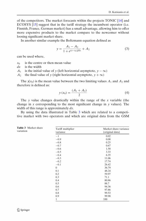
By using the data illustrated in Table 3 which are related to a competi-tive market with two operators and which are original data from the GSM

Table 3 Market sharevariation

Tariff multiplier Market share variancevariance (original data)

−1 0.02−0.9 0.08−0.8 0.25−0.7 0.67−0.6 1.58−0.5 3.33−0.4 6.35−0.3 11.06−0.2 17.74−0.1 26.420 36.790.1 48.240.2 59.970.3 71.10.4 80.860.5 88.70.6 94.360.7 97.860.8 99.530.9 99.981 100

A game theory modeling approach for 3G operators

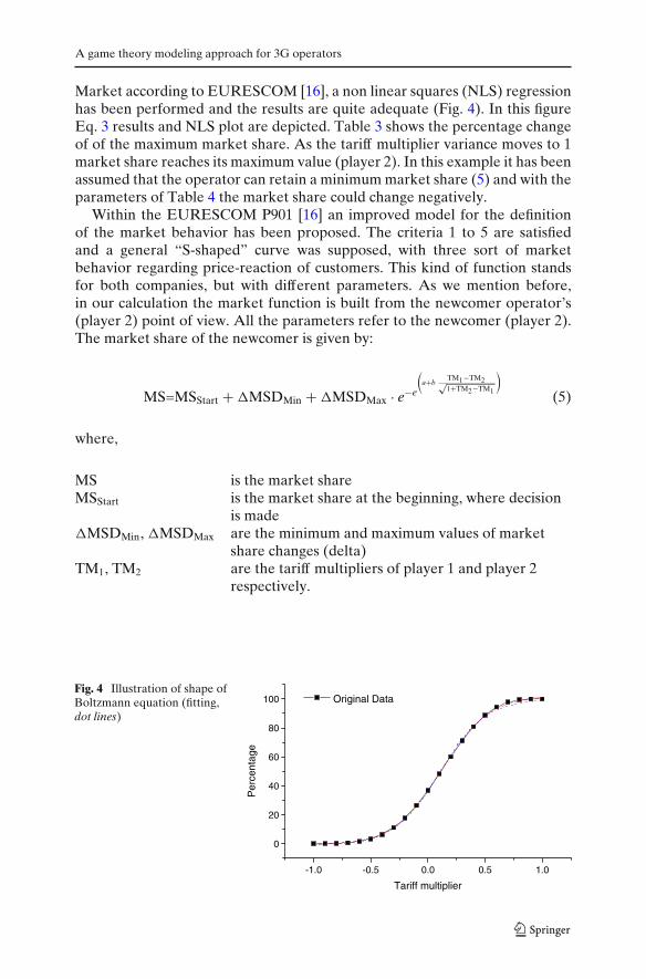
Market according to EURESCOM [16], a non linear squares (NLS) regressionhas been performed and the results are quite adequate (Fig. 4). In this figureEq. 3 results and NLS plot are depicted. Table 3 shows the percentage changeof of the maximum market share. As the tariff multiplier variance moves to 1market share reaches its maximum value (player 2). In this example it has beenassumed that the operator can retain a minimum market share (5) and with theparameters of Table 4 the market share could change negatively.

Within the EURESCOM P901 [16] an improved model for the definitionof the market behavior has been proposed. The criteria 1 to 5 are satisfiedand a general “S-shaped” curve was supposed, with three sort of marketbehavior regarding price-reaction of customers. This kind of function standsfor both companies, but with different parameters. As we mention before,in our calculation the market function is built from the newcomer operator’s(player 2) point of view. All the parameters refer to the newcomer (player 2).The market share of the newcomer is given by:

MS=MSStart + �MSDMin + �MSDMax · e−e

(a+b

TM1−TM2√1+TM2−TM1

)

(5)

where,

MS is the market shareMSStart is the market share at the beginning, where decision

is made�MSDMin, �MSDMax are the minimum and maximum values of market

share changes (delta)TM1, TM2 are the tariff multipliers of player 1 and player 2

respectively.

Fig. 4 Illustration of shape ofBoltzmann equation (fitting,dot lines)

-1.0 -0.5 0.0 0.5 1.0

0

20

40

60

80

100 Original Data

Per

cent

age

Tariff multiplier

D. Katsianis et al.

Table 4 Different versions of market parameters used in the calculation for newcomer (Player 2)

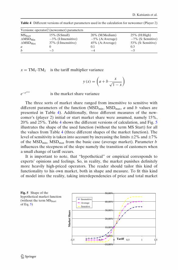
Versions: operator2 (newcomer) parameters

MSStart 15% (S:Small) 20% (M:Medium) 25% (H:High)�MSDMin −3% (I:Insensitive) −5% (A:Average) −7% (S: Sensitive)�MSDMax 37% (I:Insensitive) 45% (A:Average) 53% (S: Sensitive)a 0 0.1 0.3b −3 −4 −5

x = TM1-TM2 is the tariff multiplier variance

y (x) =(

a + bx√

1 − x

)

e−ey(x)

is the market share variance

The three sorts of market share ranged from insensitive to sensitive withdifferent parameters of the function (MSDmin, MSDmax, a and b values arepresented in Table 4). Additionally, three different measures of the new-comer’s (player 2) initial or start market share were assumed, namely 15%,20% and 25%. Table 4 shows the different versions of calculation, and Fig. 5illustrates the shape of the used function (without the term MS Start) for allthe values from Table 4 (three different shapes of the market function). Thelevel of sensitivity is taken into account by increasing the limits ±2% and ±7%of the MSDmin, MSDmax from the basic case (average market). Parameter binfluences the steepness of the slope namely the transition of customers whena small change of tariff occurs.

It is important to note, that “hypothetical” or empirical corresponds toexperts’ opinions and feelings. So, in reality, the market punishes definitelymore heavily high-priced operators. The reader should tailor this kind offunctionality to his own market, both in shape and measure. To fit this kindof model into the reality, taking interdependencies of price and total market

Fig. 5 Shape of thehypothetical market function(without the term MSStartof Eq. 5)

-10,00%

0,00%

10,00%

20,00%

30,00%

40,00%

50,00%

-1,5 -1 -0,5 0 0,5 1 1,5Tariff

Mar

ket

Shar

e

Insensitive

Average

Sensitive

A game theory modeling approach for 3G operators

size into consideration would be necessary. The parameters for the greenfieldoperator/newcomer are illustrated below:

Our hypothetical market function could be termed unfettered. It has beenfabricated in order to be realistic following the market condition alreadyproven in the GSM market. The way of achieving this kind of function may relyon time series of similar products/services history. In case of services of UMTSwe might consider GSM services. If there were analytical GSM prices–marketshares (for at least two providers) time series, we could be able to constructa simplest function for the description of the market conditions. Probably,the derived function would be simpler. In our UMTS example we assumedonly one decision point in the beginning and a 10-years long study. One coulddisagree with this approach. If we would like the approach to be closer toreality, the decision point should follow one after the other on a yearly ormonthly basis. In that case, we might use a simple function, reached from timeseries year by year. Furthermore, in gaming, the higher the number of decisionpoints, the more complex the model becomes.

The sensitivity analysis that we used and applied in UMTS BC has not beenused in constructing the hypothetical market function, but has been greatlyused in estimating the pay-offs (i.e. NPV). Following a different approach,another kind of sensitivity analysis would be (price level)/(market share),which might fruit into a simple linear function and can be used in limitedcircumstances (time frame, price-cap, market size). In our paper we have notinvestigated sensitivity in that way, but it might have fitted in market issueswhen assuming e.g. yearly decision points in the TE and GT model, and byusing results from market sensitivity functions. The next paragraph explainsthoroughly the outputs.

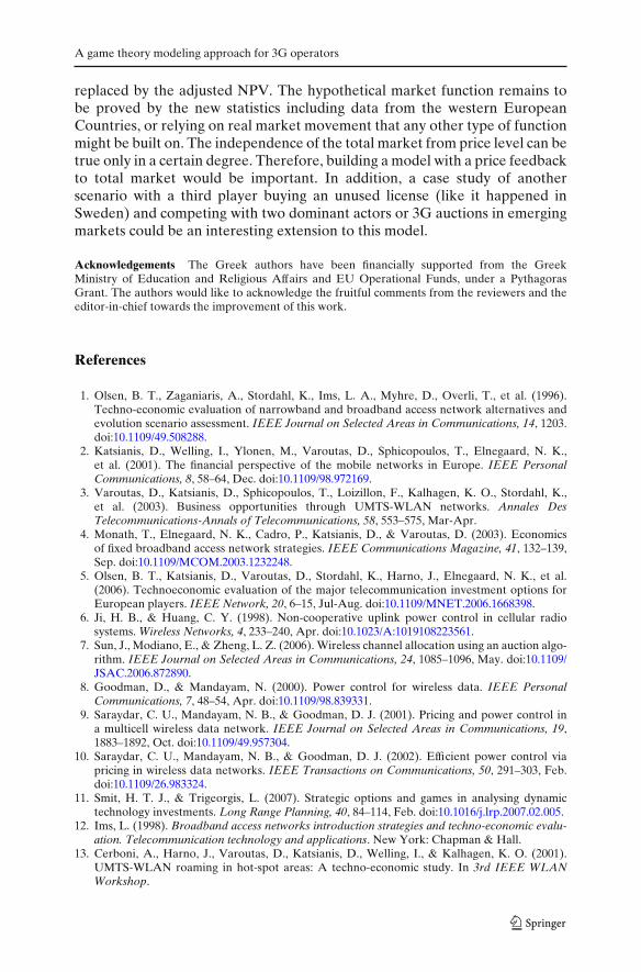
3.2 Implementation of the game

The main body of the calculations is made in MS Excel worksheets. This isalso true for market functions, tables as well as for pay-off tables. Pay-offtables stood as input of a simple translator program written on C language.The output of this little program served the GAMBIT solver with input.GAMBIT software is quite deeply explained in [19]. The results of GAMBITwere the places of Nash-equilibrium points (in this game). These points werethen drawn back to pay-off matrixes in MS Excel and TE tool.

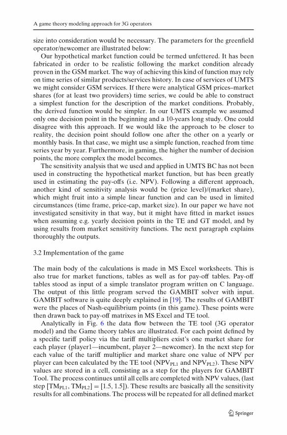
Analytically in Fig. 6 the data flow between the TE tool (3G operatormodel) and the Game theory tables are illustrated. For each point defined bya specific tariff policy via the tariff multipliers exist’s one market share foreach player (player1—incumbent, player 2—newcomer). In the next step foreach value of the tariff multiplier and market share one value of NPV perplayer can been calculated by the TE tool (NPVPL1 and NPVPL2). These NPVvalues are stored in a cell, consisting as a step for the players for GAMBITTool. The process continues until all cells are completed with NPV values, (laststep [TMPL1, TMPL2] = [1.5, 1.5]). These results are basically all the sensitivityresults for all combinations. The process will be repeated for all defined market

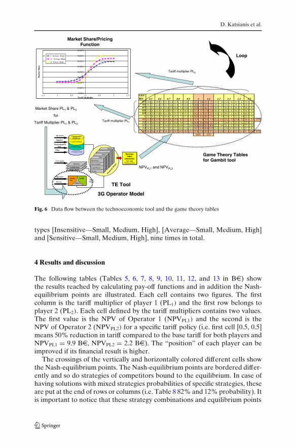
D. Katsianis et al.

GEURO

0.5 10.0 2.1 10.9 1.9 11.5 1.8 11.9 1.8 12.0 2.2 12.1 2.6 12.1 3.1 12.1 3.6 12.1 4.1 12.1 4.7 12.1 5.20.6 10.7 3.1 11.8 2.9 12.7 2.6 13.4 2.4 13.8 2.5 14.0 2.8 14.1 3.2 14.1 3.6 14.1 4.1 14.1 4.7 14.1 5.20.7 11.2 4.2 12.4 4.1 13.6 3.8 14.6 3.4 15.4 3.1 15.8 3.1 16.1 3.3 16.1 3.7 16.2 4.2 16.2 4.7 16.2 5.20.8 11.6 5.2 12.7 5.3 14.0 5.0 15.3 4.7 16.5 4.0 17.3 3.7 17.8 3.6 18.1 3.8 18.2 4.2 18.2 4.7 18.2 5.20.9 12.0 5.8 13.0 6.2 14.2 6.3 15.7 5.9 17.1 5.3 18.4 4.7 19.3 4.3 19.8 4.1 20.1 4.3 20.2 4.7 20.2 5.2

1 12.7 6.2 13.4 7.0 14.4 7.4 15.7 7.3 17.3 6.8 18.9 6.1 20.2 5.4 21.2 4.9 21.8 4.7 22.1 4.8 22.2 5.21.1 13.5 6.5 13.9 7.5 14.7 8.2 15.8 8.5 17.3 8.3 18.9 7.8 20.6 6.9 22.1 6.1 23.2 5.5 23.8 5.2 24.1 5.4 37%1.2 14.5 6.6 14.8 7.8 15.2 8.7 16.0 9.4 17.2 9.6 18.8 9.4 20.6 8.7 22.4 7.7 24.0 6.7 25.1 6.1 25.8 5.81.3 15.7 6.6 15.8 7.9 16.0 9.1 16.5 10.0 17.3 10.6 18.6 10.8 20.3 10.4 22.2 9.6 24.2 8.5 25.8 7.4 27.1 6.61.4 16.9 6.6 16.9 7.9 17.0 9.2 17.2 10.4 17.8 11.3 18.7 11.8 20.0 11.9 21.8 11.4 23.8 10.5 25.9 9.2 27.7 8.11.5 18.1 6.6 18.1 7.9 18.1 9.3 18.2 10.5 18.5 11.7 19.0 12.6 20.0 13.1 21.4 13.0 23.3 12.4 25.5 11.4 27.7 10.0 63%

88% 12%

0.5 0.6 0.7 0.8 1.3 1.4 1.50.9 1 1.1 1.2

Volume Class

OA&M Class

Cost Evolution

ComponentsDatabase

Op erators

Suppliers

Standardizationbody

Other

MarketSize

Tariffs

Policy

User inputs

Operators

Surveys

DecisionIndex

calculation(NPV, IRR,

Payback period)

Finan

cial M

odel

Year n

. . .Year 2

Revenues

Cash Flows

Profits

Investments

Year 1

Radio ModelArchitectures

Services

GameTheory

Tariff multiplier PL2

Market Share PL1 & PL2

for

Tariff Multiplier PL1 & PL2

NPVPL1 and NPVPL2

TE Tool

3G Operator Model

Tariff multiplier PL1

Game Theory Tables for Gambit tool

Loop

Market Share/PricingFunction

0,00%

10,00%

20,00%

30,00%

40,00%

50,00%

60,00%

70,00%

80,00%

-1,5 -1 -0,5 0 0,5 1 1,5Tariff Multiplier

Mar

ket

Shar

e

I - Inelastic (High)

A - Average (High)

E - Elastic (High)

Fig. 6 Data flow between the technoeconomic tool and the game theory tables

types [Insensitive—Small, Medium, High], [Average—Small, Medium, High]and [Sensitive—Small, Medium, High], nine times in total.

4 Results and discussion

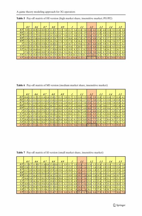
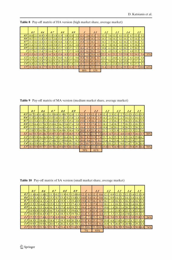
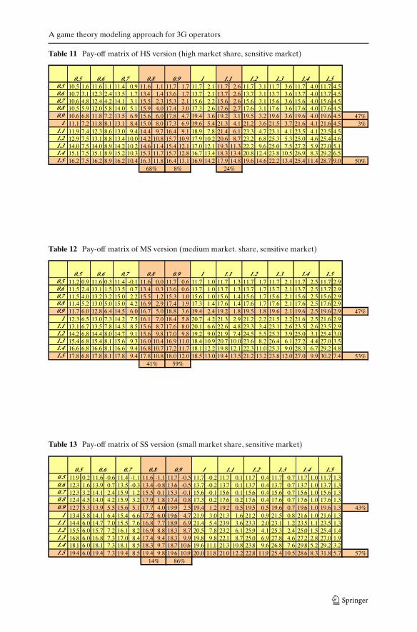
The following tables (Tables 5, 6, 7, 8, 9, 10, 11, 12, and 13 in Be) showthe results reached by calculating pay-off functions and in addition the Nash-equilibrium points are illustrated. Each cell contains two figures. The firstcolumn is the tariff multiplier of player 1 (PL1) and the first row belongs toplayer 2 (PL2). Each cell defined by the tariff multipliers contains two values.The first value is the NPV of Operator 1 (NPVPL1) and the second is theNPV of Operator 2 (NPVPL2) for a specific tariff policy (i.e. first cell [0.5, 0.5]means 50% reduction in tariff compared to the base tariff for both players andNPVPL1 = 9.9 Be, NPVPL2 = 2.2 Be). The “position” of each player can beimproved if its financial result is higher.

The crossings of the vertically and horizontally colored different cells showthe Nash-equilibrium points. The Nash-equilibrium points are bordered differ-ently and so do strategies of competitors bound to the equilibrium. In case ofhaving solutions with mixed strategies probabilities of specific strategies, theseare put at the end of rows or columns (i.e. Table 8 82% and 12% probability). Itis important to notice that these strategy combinations and equilibrium points

A game theory modeling approach for 3G operators

Table 5 Pay-off matrix of HI version (high market share, insensitive market; Pl1/Pl2)

0.5 9.9 2.2 10.5 2.4 10.9 2.5 11.2 2.7 11.5 3.0 11.7 3.4 11.8 3.8 11.8 4.2 11.8 4.8 11.8 5.3 11.8 5.80.6 11.0 2.8 11.7 3.0 12.3 3.2 12.8 3.3 13.2 3.4 13.5 3.6 13.6 3.9 13.7 4.3 13.8 4.8 13.8 5.3 13.8 5.80.7 12.0 3.5 12.7 3.8 13.5 3.9 14.1 4.0 14.7 4.0 15.1 4.0 15.4 4.2 15.6 4.5 15.7 4.9 15.8 5.3 15.8 5.80.8 12.8 4.2 13.6 4.6 14.4 4.8 15.2 4.7 15.9 4.7 16.6 4.6 17.0 4.7 17.4 4.8 17.6 5.1 17.7 5.5 17.8 5.90.9 13.5 4.7 14.3 5.2 15.2 5.5 16.1 5.6 17.0 5.5 17.8 5.4 18.4 5.3 19.0 5.3 19.3 5.4 19.6 5.6 19.7 6.0

1 14.3 5.2 15.0 5.8 15.8 6.2 16.8 6.4 17.7 6.4 18.7 6.3 19.6 6.1 20.3 6.0 20.9 5.9 21.3 6.0 21.5 6.21.1 15.2 5.5 15.7 6.3 16.5 6.9 17.3 7.2 18.4 7.4 19.4 7.3 20.5 7.1 21.4 6.8 22.2 6.6 22.8 6.5 23.2 6.61.2 16.3 5.6 16.6 6.6 17.1 7.4 17.9 8.0 18.9 8.3 19.9 8.3 21.1 8.2 22.2 7.9 23.2 7.6 24.1 7.3 24.7 7.2 17.4 5.7 17.6 6.8 18.0 7.8 18.6 8.5 19.4 9.1 20.4 9.3 21.5 9.3 22.8 9.0 24.0 8.7 25.0 8.3 25.9 8.01.4 18.7 5.8 18.8 6.9 18.9 8.0 19.3 9.0 20.0 9.7 20.8 10.1 21.9 10.3 23.1 10.2 24.4 9.9 25.7 9.5 26.8 9.01.5 20.0 5.8 20.0 7.0 20.1 8.1 20.3 9.2 20.7 10.1 21.4 10.8 22.3 11.2 23.4 11.3 24.7 11.2 26.1 10.8 27.4 10.3

1.3 1.4 1.50.9 1 1.1 1.20.5 0.6 0.7 0.8

Table 6 Pay-off matrix of MI version (medium market share, insensitive market)

0.5 10.6 1.5 11.2 1.5 11.6 1.6 12.0 1.7 11.5 2.0 11.7 2.2 11.8 2.5 11.8 2.9 11.8 3.3 11.8 3.7 11.8 4.20.6 11.8 2.1 12.5 2.2 13.1 2.2 13.6 2.2 14.0 2.3 13.5 2.5 13.6 2.7 13.7 3.0 13.8 3.3 13.8 3.8 13.8 4.20.7 12.8 2.7 13.6 2.9 14.3 2.9 15.0 2.9 15.6 2.9 16.0 2.9 15.4 3.0 15.6 3.2 15.7 3.4 15.8 3.8 15.8 4.20.8 13.7 3.3 14.5 3.6 15.4 3.7 16.2 3.7 16.9 3.6 17.5 3.5 18.0 3.4 17.4 3.5 17.6 3.6 17.7 3.9 17.8 4.30.9 14.6 3.9 15.3 4.4 16.2 4.6 17.1 4.6 18.0 4.4 18.8 4.2 19.5 4.0 20.0 3.9 19.3 4.0 19.6 4.1 19.7 4.4

1 15.5 4.4 16.1 5.0 17.0 5.3 17.9 5.4 18.9 5.3 19.8 5.1 20.7 4.8 21.4 4.6 22.0 4.5 21.3 4.5 21.5 4.61.1 16.5 4.7 17.0 5.5 17.7 6.0 18.6 6.2 19.6 6.3 20.6 6.1 21.7 5.8 22.6 5.5 23.4 5.2 24.0 5.0 23.2 5.01.2 17.6 4.9 17.9 5.8 18.5 6.5 19.2 7.0 20.2 7.2 21.3 7.1 22.4 6.9 23.5 6.5 24.5 6.1 25.4 5.8 26.0 5.51.3 18.8 5.0 19.0 6.0 19.4 6.9 20.0 7.6 20.8 8.0 21.8 8.1 22.9 8.0 24.2 7.7 25.4 7.2 26.4 6.7 27.3 6.31.4 20.2 5.1 20.2 6.1 20.4 7.1 20.8 8.0 21.4 8.6 22.3 9.0 23.4 9.0 24.6 8.8 25.9 8.4 27.2 7.9 28.3 7.41.5 21.6 5.1 21.6 6.1 21.7 7.2 21.9 8.2 22.3 9.1 22.9 9.6 23.9 10.0 25.0 10.0 26.3 9.7 27.7 9.2 29.0 8.6

0.5 0.6 0.7 0.8 1.3 1.4 1.50.9 1 1.1 1.2

Table 7 Pay-off matrix of SI version (small market share, insensitive market)

0.5 11.3 0.7 11.9 0.7 11.6 0.6 12.0 0.6 11.5 0.9 11.7 1.0 11.8 1.2 11.8 1.5 11.8 1.9 11.8 2.2 11.8 2.60.6 12.6 1.3 13.3 1.3 13.9 1.2 13.6 1.1 14.0 1.2 13.5 1.3 13.6 1.4 13.7 1.6 13.8 1.9 13.8 2.2 13.8 2.60.7 13.7 2.0 14.5 2.0 15.2 2.0 15.9 1.8 15.6 1.8 16.0 1.7 15.4 1.7 15.6 1.8 15.7 2.0 15.8 2.3 15.8 2.60.8 14.7 2.6 15.5 2.8 16.3 2.8 17.1 2.6 17.9 2.5 17.5 2.3 18.0 2.1 17.4 2.1 17.6 2.2 17.7 2.4 17.8 2.60.9 15.6 3.1 16.4 3.5 17.3 3.6 18.2 3.6 19.1 3.3 19.9 3.0 19.5 2.8 20.0 2.6 19.3 2.5 19.6 2.6 19.7 2.8

1 16.6 3.6 17.3 4.2 18.1 4.5 19.0 4.5 20.0 4.2 21.0 3.9 21.9 3.6 21.4 3.2 22.0 3.0 21.3 2.9 21.5 3.01.1 17.7 3.9 18.2 4.7 18.9 5.1 19.8 5.2 20.8 5.2 21.9 4.9 22.9 4.5 23.9 4.1 23.4 3.7 24.0 3.5 23.2 3.31.2 18.9 4.1 19.2 5.0 19.8 5.6 20.5 6.0 21.5 6.1 22.6 6.0 23.7 5.6 24.8 5.2 25.8 4.7 25.4 4.2 26.0 3.91.3 20.2 4.2 20.4 5.2 20.8 6.0 21.4 6.6 22.2 6.9 23.2 6.9 24.4 6.7 25.6 6.3 26.8 5.8 27.8 5.2 27.3 4.71.4 21.7 4.3 21.7 5.3 21.9 6.2 22.3 7.0 22.9 7.5 23.8 7.8 24.9 7.8 26.1 7.5 27.4 7.0 28.7 6.4 29.8 5.71.5 23.2 4.3 23.2 5.3 23.3 6.3 23.4 7.2 23.9 8.0 24.5 8.5 25.4 8.7 26.6 8.6 27.9 8.3 29.3 7.7 30.6 7.0

1.3 1.4 1.50.9 1 1.1 1.20.5 0.6 0.7 0.8

D. Katsianis et al.

Table 8 Pay-off matrix of HA version (high market share, average market)

0.5 10.0 2.1 10.9 1.9 11.5 1.8 11.9 1.8 12.0 2.2 12.1 2.6 12.1 3.1 12.1 3.6 12.1 4.1 12.1 4.7 12.1 5.20.6 10.7 3.1 11.8 2.9 12.7 2.6 13.4 2.4 13.8 2.5 14.0 2.8 14.1 3.2 14.1 3.6 14.1 4.1 14.1 4.7 14.1 5.20.7 11.2 4.2 12.4 4.1 13.6 3.8 14.6 3.4 15.4 3.1 15.8 3.1 16.1 3.3 16.1 3.7 16.2 4.2 16.2 4.7 16.2 5.20.8 11.6 5.2 12.7 5.3 14.0 5.0 15.3 4.7 16.5 4.0 17.3 3.7 17.8 3.6 18.1 3.8 18.2 4.2 18.2 4.7 18.2 5.20.9 12.0 5.8 13.0 6.2 14.2 6.3 15.7 5.9 17.1 5.3 18.4 4.7 19.3 4.3 19.8 4.1 20.1 4.3 20.2 4.7 20.2 5.2

1 12.7 6.2 13.4 7.0 14.4 7.4 15.7 7.3 17.3 6.8 18.9 6.1 20.2 5.4 21.2 4.9 21.8 4.7 22.1 4.8 22.2 5.21.1 13.5 6.5 13.9 7.5 14.7 8.2 15.8 8.5 17.3 8.3 18.9 7.8 20.6 6.9 22.1 6.1 23.2 5.5 23.8 5.2 24.1 5.4 37%1.2 14.5 6.6 14.8 7.8 15.2 8.7 16.0 9.4 17.2 9.6 18.8 9.4 20.6 8.7 22.4 7.7 24.0 6.7 25.1 6.1 25.8 5.81.3 15.7 6.6 15.8 7.9 16.0 9.1 16.5 10.0 17.3 10.6 18.6 10.8 20.3 10.4 22.2 9.6 24.2 8.5 25.8 7.4 27.1 6.61.4 16.9 6.6 16.9 7.9 17.0 9.2 17.2 10.4 17.8 11.3 18.7 11.8 20.0 11.9 21.8 11.4 23.8 10.5 25.9 9.2 27.7 8.11.5 18.1 6.6 18.1 7.9 18.1 9.3 18.2 10.5 18.5 11.7 19.0 12.6 20.0 13.1 21.4 13.0 23.3 12.4 25.5 11.4 27.7 10.0 63%

88% 12%

0.5 0.6 0.7 0.8 1.3 1.4 1.50.9 1 1.1 1.2

Table 9 Pay-off matrix of MA version (medium market share, average market)

0.5 10.7 1.4 11.6 1.1 11.5 0.8 11.9 0.7 12.0 1.1 12.1 1.5 12.1 1.9 12.1 2.3 12.1 2.7 12.1 3.1 12.1 3.50.6 11.5 2.4 12.6 2.1 13.5 1.6 13.4 1.3 13.8 1.4 14.0 1.6 14.1 1.9 14.1 2.3 14.1 2.7 14.1 3.1 14.1 3.50.7 12.1 3.4 13.2 3.2 14.4 2.8 15.5 2.3 15.4 2.0 15.8 1.9 16.1 2.0 16.1 2.3 16.2 2.7 16.2 3.1 16.2 3.50.8 12.5 4.4 13.7 4.5 15.0 4.2 16.3 3.6 17.4 3.0 17.3 2.5 17.8 2.3 18.1 2.4 18.2 2.7 18.2 3.1 18.2 3.50.9 13.1 5.1 14.0 5.4 15.3 5.4 16.7 4.9 18.2 4.3 19.4 3.5 19.3 3.0 19.8 2.8 20.1 2.9 20.2 3.2 20.2 3.5

1 13.8 5.5 14.5 6.2 15.5 6.5 16.9 6.3 18.4 5.8 20.0 4.9 21.4 4.1 21.2 3.5 21.8 3.2 22.1 3.3 22.2 3.61.1 14.7 5.7 15.2 6.7 15.9 7.3 17.0 7.5 18.5 7.3 20.2 6.6 21.9 5.6 23.3 4.7 23.2 4.0 23.8 3.7 24.1 3.7 30%1.2 15.9 5.9 16.1 6.9 16.5 7.8 17.3 8.4 18.5 8.5 20.1 8.2 21.9 7.4 23.7 6.3 25.3 5.3 25.1 4.5 25.8 4.21.3 17.1 5.9 17.2 7.1 17.4 8.2 17.9 9.0 18.7 9.5 20.0 9.6 21.7 9.1 23.6 8.2 25.6 7.0 27.2 5.9 27.1 5.01.4 18.4 5.9 18.4 7.1 18.5 8.3 18.7 9.4 19.3 10.2 20.2 10.7 21.5 10.6 23.3 10.1 25.3 9.0 27.4 7.7 29.2 6.41.5 18.1 5.9 19.7 7.1 19.7 8.4 19.8 9.5 20.1 10.6 20.6 11.4 21.6 11.8 23.0 11.7 24.9 11.0 27.1 9.8 29.2 8.4 70%

1.3 1.4 1.50.9 1 1.1 1.2

39% 61%

0.5 0.6 0.7 0.8

Table 10 Pay-off matrix of SA version (small market share, average market)

0.5 11.4 0.6 11.6 0.2 11.5 -0.2 11.9 -0.3 12.0 0.0 12.1 0.3 12.1 0.6 12.1 0.9 12.1 1.2 12.1 1.6 12.1 1.90.6 12.3 1.6 13.4 1.2 13.5 0.7 13.4 0.2 13.8 0.3 14.0 0.4 14.1 0.6 14.1 0.9 14.1 1.2 14.1 1.6 14.1 1.90.7 12.9 2.6 14.1 2.4 15.3 1.8 15.5 1.2 15.4 0.9 15.8 0.7 16.1 0.7 16.1 1.0 16.2 1.3 16.2 1.6 16.2 1.90.8 13.5 3.5 14.6 3.5 15.9 3.2 17.3 2.5 17.4 1.9 17.3 1.3 17.8 1.1 18.1 1.1 18.2 1.3 18.2 1.6 18.2 1.90.9 14.1 4.3 15.1 4.6 16.3 4.5 17.8 4.0 19.2 3.2 19.4 2.4 19.3 1.7 19.8 1.4 20.1 1.4 20.2 1.6 20.2 1.9

1 14.9 4.8 15.6 5.4 16.7 5.6 18.0 5.3 19.6 4.7 21.1 3.8 21.4 2.8 21.2 2.1 21.8 1.8 22.1 1.8 22.2 2.01.1 16.0 5.0 16.4 5.8 17.1 6.4 18.3 6.5 19.7 6.2 21.4 5.4 23.1 4.4 23.3 3.3 23.2 2.6 23.8 2.2 24.1 2.11.2 17.2 5.2 17.4 6.1 17.8 6.9 18.6 7.4 19.8 7.5 21.4 7.0 23.2 6.1 25.0 5.0 25.3 3.8 25.1 3.0 25.8 2.5 26%1.3 18.5 5.2 18.6 6.3 18.8 7.2 19.3 8.0 20.2 8.4 21.4 8.4 23.1 7.9 25.0 6.8 27.0 5.6 27.2 4.3 27.1 3.41.4 19.9 5.2 19.9 6.3 20.0 7.4 20.2 8.4 20.7 9.1 21.7 9.5 23.0 9.4 24.8 8.7 26.8 7.6 28.9 6.2 29.2 4.81.5 19.7 5.2 21.3 6.3 21.3 7.4 21.4 8.5 21.6 9.5 22.2 10.2 23.2 10.5 24.6 10.3 26.5 9.5 28.6 8.3 30.8 6.8 74%

7% 93%

0.5 0.6 0.7 0.8 1.3 1.4 1.50.9 1 1.1 1.2

A game theory modeling approach for 3G operators

Table 11 Pay-off matrix of HS version (high market share, sensitive market)

0.5 10.5 1.6 11.6 1.1 11.4 0.9 11.6 1.1 11.7 1.7 11.7 2.1 11.7 2.6 11.7 3.1 11.7 3.6 11.7 4.0 11.7 4.50.6 10.7 3.1 12.3 2.4 13.5 1.7 13.4 1.4 13.6 1.7 13.7 2.1 13.7 2.6 13.7 3.1 13.7 3.6 13.7 4.0 13.7 4.50.7 10.6 4.8 12.4 4.2 14.1 3.1 15.5 2.3 15.3 2.1 15.6 2.2 15.6 2.6 15.6 3.1 15.6 3.6 15.6 4.0 15.6 4.50.8 10.5 5.9 12.0 5.8 14.0 5.1 15.9 4.0 17.4 3.0 17.3 2.6 17.6 2.7 17.6 3.1 17.6 3.6 17.6 4.0 17.6 4.50.9 10.6 6.8 11.8 7.2 13.5 6.9 15.6 6.0 17.8 4.7 19.4 3.6 19.2 3.1 19.5 3.2 19.6 3.6 19.6 4.0 19.6 4.5 47%

1 11.1 7.2 11.8 8.1 13.1 8.4 15.0 8.0 17.3 6.9 19.6 5.4 21.3 4.1 21.2 3.6 21.5 3.7 21.6 4.1 21.6 4.5 3%1.1 11.9 7.4 12.3 8.6 13.0 9.4 14.4 9.7 16.4 9.1 18.9 7.8 21.4 6.1 23.3 4.7 23.1 4.1 23.5 4.1 23.5 4.51.2 12.9 7.5 13.1 8.8 13.4 10.0 14.2 10.8 15.7 10.9 17.9 10.2 20.6 8.7 23.2 6.8 25.3 5.3 25.0 4.6 25.4 4.61.3 14.0 7.5 14.0 8.9 14.2 10.2 14.6 11.4 15.4 12.1 17.0 12.1 19.3 11.3 22.2 9.6 25.0 7.5 27.2 5.9 27.0 5.11.4 15.1 7.5 15.1 8.9 15.2 10.3 15.3 11.7 15.7 12.8 16.7 13.4 18.3 13.4 20.8 12.4 23.8 10.5 26.9 8.3 29.2 6.51.5 16.2 7.5 16.2 8.9 16.2 10.4 16.3 11.8 16.4 13.1 16.9 14.2 17.9 14.8 19.6 14.6 22.2 13.4 25.4 11.4 28.7 9.0 50%

68% 8% 24%

0.5 0.6 0.7 0.8 1.3 1.4 1.50.9 1 1.1 1.2

Table 12 Pay-off matrix of MS version (medium market. share, sensitive market)

0.5 11.2 0.9 11.6 0.3 11.4 -0.1 11.6 0.0 11.7 0.6 11.7 1.0 11.7 1.3 11.7 1.7 11.7 2.1 11.7 2.5 11.7 2.90.6 11.5 2.4 13.1 1.5 13.5 0.7 13.4 0.3 13.6 0.6 13.7 1.0 13.7 1.3 13.7 1.7 13.7 2.1 13.7 2.5 13.7 2.90.7 11.5 4.0 13.2 3.2 15.0 2.2 15.5 1.2 15.3 1.0 15.6 1.0 15.6 1.4 15.6 1.7 15.6 2.1 15.6 2.5 15.6 2.90.8 11.4 5.2 13.0 5.0 15.0 4.2 16.9 2.9 17.4 1.9 17.3 1.4 17.6 1.4 17.6 1.7 17.6 2.1 17.6 2.5 17.6 2.90.9 11.7 6.0 12.8 6.4 14.5 6.0 16.7 5.0 18.8 3.6 19.4 2.4 19.2 1.8 19.5 1.8 19.6 2.1 19.6 2.5 19.6 2.9 47%

1 12.3 6.5 13.0 7.3 14.2 7.5 16.1 7.0 18.4 5.8 20.7 4.2 21.3 2.9 21.2 2.2 21.5 2.2 21.6 2.5 21.6 2.91.1 13.1 6.7 13.5 7.8 14.3 8.5 15.6 8.7 17.6 8.0 20.1 6.6 22.6 4.8 23.3 3.4 23.1 2.6 23.5 2.6 23.5 2.91.2 14.2 6.8 14.4 8.0 14.7 9.1 15.6 9.8 17.0 9.8 19.2 9.0 21.9 7.4 24.5 5.5 25.3 3.9 25.0 3.1 25.4 3.01.3 15.4 6.8 15.4 8.1 15.6 9.3 16.0 10.4 16.9 11.0 18.4 10.9 20.7 10.0 23.6 8.2 26.4 6.1 27.2 4.4 27.0 3.51.4 16.6 6.8 16.6 8.1 16.6 9.4 16.8 10.7 17.2 11.7 18.1 12.2 19.8 12.1 22.3 11.0 25.3 9.0 28.3 6.7 29.2 4.81.5 17.8 6.8 17.8 8.1 17.8 9.4 17.8 10.8 18.0 12.0 18.5 13.0 19.4 13.5 21.2 13.2 23.8 12.0 27.0 9.9 30.2 7.4 53%

1 1.21.1 1.3 1.4 1.5

41% 59%

0.5 0.6 0.7 0.8 0.9

Table 13 Pay-off matrix of SS version (small market share, sensitive market)

0.5 11.9 0.2 11.6 -0.6 11.4 -1.1 11.6 -1.1 11.7 -0.5 11.7 -0.2 11.7 0.1 11.7 0.4 11.7 0.7 11.7 1.0 11.7 1.30.6 12.3 1.6 13.9 0.7 13.5 -0.3 13.4 -0.8 13.6 -0.5 13.7 -0.2 13.7 0.1 13.7 0.4 13.7 0.7 13.7 1.0 13.7 1.30.7 12.3 3.2 14.1 2.4 15.9 1.2 15.5 0.1 15.3 -0.1 15.6 -0.1 15.6 0.1 15.6 0.4 15.6 0.7 15.6 1.0 15.6 1.30.8 12.4 4.5 14.0 4.2 15.9 3.2 17.9 1.8 17.4 0.8 17.3 0.2 17.6 0.2 17.6 0.4 17.6 0.7 17.6 1.0 17.6 1.30.9 12.7 5.3 13.9 5.5 15.6 5.1 17.7 4.0 19.9 2.5 19.4 1.2 19.2 0.5 19.5 0.5 19.6 0.7 19.6 1.0 19.6 1.3 43%

1 13.4 5.8 14.1 6.4 15.4 6.6 17.2 6.0 19.6 4.7 21.9 3.0 21.3 1.6 21.2 0.9 21.5 0.8 21.6 1.0 21.6 1.31.1 14.4 6.0 14.7 7.0 15.5 7.6 16.8 7.7 18.9 6.9 21.4 5.4 23.9 3.6 23.3 2.0 23.1 1.2 23.5 1.1 23.5 1.31.2 15.5 6.0 15.7 7.2 16.1 8.2 16.9 8.8 18.3 8.7 20.5 7.8 23.2 6.1 25.9 4.1 25.3 2.4 25.0 1.5 25.4 1.41.3 16.8 6.0 16.8 7.3 17.0 8.4 17.4 9.4 18.3 9.9 19.8 9.8 22.1 8.7 25.0 6.9 27.8 4.6 27.2 2.8 27.0 1.91.4 18.1 6.0 18.1 7.3 18.1 8.5 18.3 9.7 18.7 10.6 19.6 11.1 21.3 10.8 23.8 9.6 26.8 7.6 29.8 5.2 29.2 3.21.5 19.4 6.0 19.4 7.3 19.4 8.5 19.4 9.8 19.6 10.9 20.0 11.8 21.0 12.2 22.8 11.9 25.4 10.5 28.6 8.3 31.8 5.7 57%

0.5 0.6 0.7 0.8 1.4 1.5

14% 86%

0.9 1 1.21.1 1.3

D. Katsianis et al.

should be seen as being Nash-sense, and even if we might speak about strategylikely to be followed, the general meaning of this is different from a “dominantstrategy”.

Having Nash-sense equilibrium practically means both competitors playtheir best strategy, related to the other strategies selected. This can be doneonly in such a way, that players know each other’s strategy in advance. Withinspecific limits, this could be a real situation taking also into account theregulatory obligations for specific roll-out plans. Formation of mixed strategiesas solutions means that unambiguous or simple strategies do not exist in orderto reach an equilibrium. Of course, the reader might define other kinds ofequilibrium condition than Nash-sense, e.g. managers may be interested instrategy being “the best” independent of other players’ strategy-selection,or what happens if all the other players work the ruin of the others. Inthe first case, “dominant strategy” can be reached while in the second case,operators would have in their hands “the safe strategy”; so both being a kindof equilibrium.

Falling back on the Nash-equilibrium points, and having mixed strategy so-lutions, the operators should play on a “statistical base”, and choose strategiesrelying on numerical possibilities. As this seems to be rather “unrealistic”,operators would likely follow a strategy of higher probability value.

Quite independently of the initial market share of the newcomer and thetype of market, the newcomer has to have always smaller prices, as the marketanalyzer might feel that this is “natural”. In most of our results this offers quitesmall tariffs compared to the incumbent operator’s ones.

As the initial market share of newcomer increases, both competitors shoulddecrease their prices, but regarding our inelastic total market models, incum-bent always has a chance of having “the highest” price, being viable at thesame time (quite positive NPV). This is true due to shape of the market sharefunction that has been derived from the original data (Table 3) and due to thefact that the incumbent operator has larger initial market share.

It is interesting that with increasing sensibility of the market the solutionsexist only with mixed strategies. This means that the mutual impact of com-petitors on each other, assumes that players have investigated what the otherplayer does, deeply into statistical decision making “process”.

These ideas above were only initial ones, and the reader should feel free todraw deeper experiences.

5 Conclusions and further topics

As far as game theory is concerned the investigated model served mainlyas a simple but good illustrative example to show the UMTS business situ-ation with competition among operators. It contains quite some limitations,but it succeeded in illustrating how competitors might effect on each other.Incorporation of real options into the calculation would be possible in thetechnoeconomic tool in the latest version [15]. In this case, NPV should be

A game theory modeling approach for 3G operators

replaced by the adjusted NPV. The hypothetical market function remains tobe proved by the new statistics including data from the western EuropeanCountries, or relying on real market movement that any other type of functionmight be built on. The independence of the total market from price level can betrue only in a certain degree. Therefore, building a model with a price feedbackto total market would be important. In addition, a case study of anotherscenario with a third player buying an unused license (like it happened inSweden) and competing with two dominant actors or 3G auctions in emergingmarkets could be an interesting extension to this model.

Acknowledgements The Greek authors have been financially supported from the GreekMinistry of Education and Religious Affairs and EU Operational Funds, under a PythagorasGrant. The authors would like to acknowledge the fruitful comments from the reviewers and theeditor-in-chief towards the improvement of this work.

References

1. Olsen, B. T., Zaganiaris, A., Stordahl, K., Ims, L. A., Myhre, D., Overli, T., et al. (1996).Techno-economic evaluation of narrowband and broadband access network alternatives andevolution scenario assessment. IEEE Journal on Selected Areas in Communications, 14, 1203.doi:10.1109/49.508288.

2. Katsianis, D., Welling, I., Ylonen, M., Varoutas, D., Sphicopoulos, T., Elnegaard, N. K.,et al. (2001). The financial perspective of the mobile networks in Europe. IEEE PersonalCommunications, 8, 58–64, Dec. doi:10.1109/98.972169.

3. Varoutas, D., Katsianis, D., Sphicopoulos, T., Loizillon, F., Kalhagen, K. O., Stordahl, K.,et al. (2003). Business opportunities through UMTS-WLAN networks. Annales DesTelecommunications-Annals of Telecommunications, 58, 553–575, Mar-Apr.

4. Monath, T., Elnegaard, N. K., Cadro, P., Katsianis, D., & Varoutas, D. (2003). Economicsof fixed broadband access network strategies. IEEE Communications Magazine, 41, 132–139,Sep. doi:10.1109/MCOM.2003.1232248.

5. Olsen, B. T., Katsianis, D., Varoutas, D., Stordahl, K., Harno, J., Elnegaard, N. K., et al.(2006). Technoeconomic evaluation of the major telecommunication investment options forEuropean players. IEEE Network, 20, 6–15, Jul-Aug. doi:10.1109/MNET.2006.1668398.

6. Ji, H. B., & Huang, C. Y. (1998). Non-cooperative uplink power control in cellular radiosystems. Wireless Networks, 4, 233–240, Apr. doi:10.1023/A:1019108223561.

7. Sun, J., Modiano, E., & Zheng, L. Z. (2006). Wireless channel allocation using an auction algo-rithm. IEEE Journal on Selected Areas in Communications, 24, 1085–1096, May. doi:10.1109/JSAC.2006.872890.

8. Goodman, D., & Mandayam, N. (2000). Power control for wireless data. IEEE PersonalCommunications, 7, 48–54, Apr. doi:10.1109/98.839331.

9. Saraydar, C. U., Mandayam, N. B., & Goodman, D. J. (2001). Pricing and power control ina multicell wireless data network. IEEE Journal on Selected Areas in Communications, 19,1883–1892, Oct. doi:10.1109/49.957304.

10. Saraydar, C. U., Mandayam, N. B., & Goodman, D. J. (2002). Efficient power control viapricing in wireless data networks. IEEE Transactions on Communications, 50, 291–303, Feb.doi:10.1109/26.983324.

11. Smit, H. T. J., & Trigeorgis, L. (2007). Strategic options and games in analysing dynamictechnology investments. Long Range Planning, 40, 84–114, Feb. doi:10.1016/j.lrp.2007.02.005.

12. Ims, L. (1998). Broadband access networks introduction strategies and techno-economic evalu-ation. Telecommunication technology and applications. New York: Chapman & Hall.

13. Cerboni, A., Harno, J., Varoutas, D., Katsianis, D., Welling, I., & Kalhagen, K. O. (2001).UMTS-WLAN roaming in hot-spot areas: A techno-economic study. In 3rd IEEE WLANWorkshop.

D. Katsianis et al.

14. IST-TONIC (2000). Techno-economics of IP Optimised Networks and Services. Brussels: EU.15. CELTIC-ECOSYS (2002). Techno-ECOnomics of integrated communication SYStems and

services. Helsinki: CELTIC.16. EURESCOM (2001). EURESCOM-P901 (European Institute for Research and Strategic

Studies in Telecommunications GmbH). Heidelberg: EURESCOM.17. Olsen, B. T., & Stordahl, K. (2004). Models for forecasting cost evolution of components and

technologies. Telektronikk, 4, 138–148.18. Dixit, A. K., & Pindyck, R. S. (1994). Investment under uncertainty. Princeton: Princeton

University Press.19. McKelvey, R. D. (1997). An interactive extensive form game program. http://econweb.

tamu.edu/gambit/. California Institute of Technology.