A Fully-Connected Layered Model of Foreground and Background Flow

Deqing Sun1 Jonas Wulff2 Erik B. Sudderth3 Hanspeter Pfister1 Michael J. Black2

1Harvard University 2MPI for Intelligent Systems 3Brown University

(a) First frame of video (b) Flow field [27] (c) Segmentation [27] (d) Flow field, proposed (e) Segmentation, proposedFigure 1. The proposed fully-connected layered model can recover fine structures better than a locally connected layered model [27].

Abstract

Layered models allow scene segmentation and motionestimation to be formulated together and to inform one an-other. Traditional layered motion methods, however, employfairly weak models of scene structure, relying on locallyconnected Ising/Potts models which have limited ability tocapture long-range correlations in natural scenes. To ad-dress this, we formulate a fully-connected layered model thatenables global reasoning about the complicated segmen-tations of real objects. Optimization with fully-connectedgraphical models is challenging, and our inference algo-rithm leverages recent work on efficient mean field updatesfor fully-connected conditional random fields. These meth-ods can be implemented efficiently using high-dimensionalGaussian filtering. We combine these ideas with a layeredflow model, and find that the long-range connections greatlyimprove segmentation into figure-ground layers when com-pared with locally connected MRF models. Experiments onseveral benchmark datasets show that the method can re-cover fine structures and large occlusion regions, with goodflow accuracy and much lower computational cost than pre-vious locally-connected layered models.

1. Introduction

Layered models [8, 12, 30] are promising for motionanalysis, particularly for handling occlusion and capturingtemporally consistent scene structure [27]. Their advantagederives from the fact that they combine motion estimationwith segmentation. This allows the integration of image-based information with flow information to arrive at a goodsegmentation of the scene, which is propagated over timeusing motion cues. Accurate segmentations, and thus appro-

priate spatial segmentation and image appearance priors, arekey to achieving good performance.

Ising/Potts models produce global segmentations fromthe interaction of neighboring pixels. While popular in manyvision tasks, including layered models [31], such local de-pendencies have limited modeling power. For example, inthe “Hand” sequence of Figure 1, ambiguous local motionand boundary cues cause locally connected layered mod-els [27] to merge the background between the fingers intothe foreground (Figure 1(b)).

The problem becomes easier with the more global viewprovided by a fully-connected model that captures pairwiseinteractions among every pair of pixels. By linking thenarrow background regions between the fingers to other dis-tant background regions, it becomes far easier to correctlysegment foreground objects. Though appealing in model-ing power, these fully-connected priors are difficult to opti-mize. In this case, neither gradient-based methods [10] norgraph cuts are computationally efficient [21]. Fortunately,Krahenbuhl and Koltun [15] recently showed that mean fieldapproximation algorithms can efficiently optimize denselyconnected CRF models for static image segmentation. Mes-sage update steps are efficiently implemented via bilateralfiltering. Recent work applies their optimization scheme tooptical flow [16] by directly modeling the flow field with adensely connected CRF.

For optical flow estimation, we argue that it is more pow-erful to utilize a fully-connected prior for layer segmentation.To that end, we formulate a new model that combines re-cent work on layered flow estimation with algorithms forstatic image segmentation with fully-connected models. Theresulting objective function effectively combines informa-tion about motion, occlusion, image appearance, and time to

estimate a temporally consistent segmentation of the sceneand its evolution. Here we focus on a two-layer modeland produce figure-ground segmentations, but our methodcould be readily extended to more layers. We exploit high-dimensional Gaussian filtering to implement the spatial mes-sage passing. Because flow fields are not directly observed,optimization for fully-connected layered models is morechallenging than for static image segmentation models, andwe proposal several innovations to improve speed and ac-curacy. In spite of modeling additional dependencies, ourresulting mean field method is more efficient than previouslocally connected formulations [27].

Our key contributions are 1) a new formulation of thelayered optical flow problem that exploits a fully-connectedmodel to achieve better segmentation and that effectivelycouples image and motion segmentation; 2) a mean fieldapproximation that leverages recent work on image segmen-tation; 3) an objective function that effectively models oc-clusions to enable figure-ground segmentation; 4) a precisesegmentation of the scene into regions of foreground andbackground; 5) new schemes for optimizing fully-connectedmodels for layered motion estimation; 6) competitive resultson benchmark datasets with a relatively low computationalcost compared to locally-connected layered models.

2. Related WorkSeveral previous and current lines of research intersect

our theme, including figure-ground segmentation, video seg-mentation, and layered optical flow estimation. A review ofthese broad fields is beyond our scope. Here we focus onlayered models, and specifically ones that combine motionestimation and segmentation.

While our 2-layer method is related to figure-ground seg-mentation, previous work in that area typically uses motiononly as a cue to segmentation [7], treats it as an observation[2], and does not attempt to accurately estimate optical flow.In contrast, our work attempts to simultaneously estimateaccurate flow and solve for a figure-ground segmentationthat gives good flow estimates. Our work is also completelyautomatic, unlike much of the work on video matting, whichusually requires the user to provide a rough segmentationin the form of a trimap. Furthermore, our method can beextended beyond figure-ground to model more layers.

Recent work by Ochs and Brox [22] addresses motionsegmentation using point trajectories. They show that higher-order tuples (3-affinities) and segmentation using spectralclustering can produce nice segmentations of scenes withseveral moving objects. Unlike our work, they do not addressthe dense flow estimation problem, and consequently do nottest on competitive flow benchmarks.

Unger et al. [29] can handle scenes with hundreds oflabels and handle occlusions by an outlier process withoutgeometric modeling. The estimated motion is not very accu-

rate as evaluated on the Middlebury benchmark.

Our work is directly descended from layered models ofoptical flow [12, 30, 31]. Several methods extract layeredmodels of the scene as well as layer movement, using para-metric models of the motion of each layer. Jojic and Frey[13] extract segmented regions and reason about their depthorder, but focus on simple translational motions and do notprovide a segmentation of the scene. Kumar et al. [18]address a similar problem but exploit graph cuts for opti-mization and assume a piecewise parametric model of thescene using a purely local MRF model.

Accurate flow estimation and segmentation requiresricher models of flow within layers that go beyond simpleparametric transformations. Previous methods [27, 31] allowthe flow to vary smoothly or discontinuously within layers.Recent work [27] shows that such models can achieve goodflow and segmentation accuracy, albeit with high computa-tional cost. Layered representations are more complicatedthan commonly used MRF models, and often use a sequenceof random fields/functions [26, 27] to model depth order andocclusions. Inference is thus more challenging. A limitationof these previous methods is that the spatial variation in theflow is modeled by a local (typically pairwise, Ising or Potts)MRF.

Graph cuts (GC) [4] and belief propagation (BP) [17]are popular optimizers for Ising/Potts models and can findbetter local optima than local search methods [28]. However,local MRF models are fundamentally limited in their expres-sive power. One way to go beyond local MRFs is to usehigher-order potentials [24], but these models are difficultto optimize using GC [14] or BP [19]. Another way to addlong-range interactions is to densely connect distant pixels asin the non-local means denoising methods [5]. Such methodsdo not address layers, segmentation or flow.

Here we build on recent fully-connected models in whichevery pixel is connected to every other pixel. Krahenbuhland Koltun [15] describe a mean-field approximate inferencescheme for fully connected CRF models. They show that thespatial message passing step can be efficiently approximatedby high-dimensional filtering [1]. Zhang and Chen [33] in-dependently suggest a quadratic programming relaxation forfully connected CRFs, and use bilateral filtering to performgradient descent. Our main contribution is to extend thesefully-connected inference methods to layered models foroptical flow estimation and segmentation.

3. Fully Connected Modeling and Inference

We first formulate our fully connected layered model, andthen describe a variational expectation maximization (EM)inference algorithm.

3.1. A Fully Connected Layered Flow Model

Given a sequence of images It, 1 ≤ t ≤ T , we seek to de-compose the scene into foreground (k=1) and background(k=2) layers. We use the terms foreground and backgroundloosely; the foreground layer is one that contains regions oc-cluding the background. Generally, multiple moving objectsthat do not mutually occlude each other will appear in theforeground layer. A multi-layer formulation [26] can lead tosemantically more meaningful segmentations of the scenebut is beyond the scope of this paper. Experimentally we findthat complex scenes can be surprisingly well approximatedby a two-layer model.

Each layer k has its own flow field (utk,vtk). We use asemi-parametric flow model [27] that biases the flow withineach layer to be piecewise smooth, and roughly similar to aglobal affine motion. For the horizontal flow field, utk, wedefine the spatial energy term, Emrf(utk, θtk) =∑

(p,q)∈Emrf

ρmrf (uptk−uqtk)+λaff

∑p

ρaff(uptk−u

pθtk

), (1)

where p and q are pixel indices, Emrf contains spatial edgesconnecting the four nearest pixels, ρ(·) is a robust penaltyfunction, λaff is a weight, and uθtk is the horizontal com-ponent of an affine motion within the layer. The energyfunction for vtk, the vertical flow field, is defined similarly.

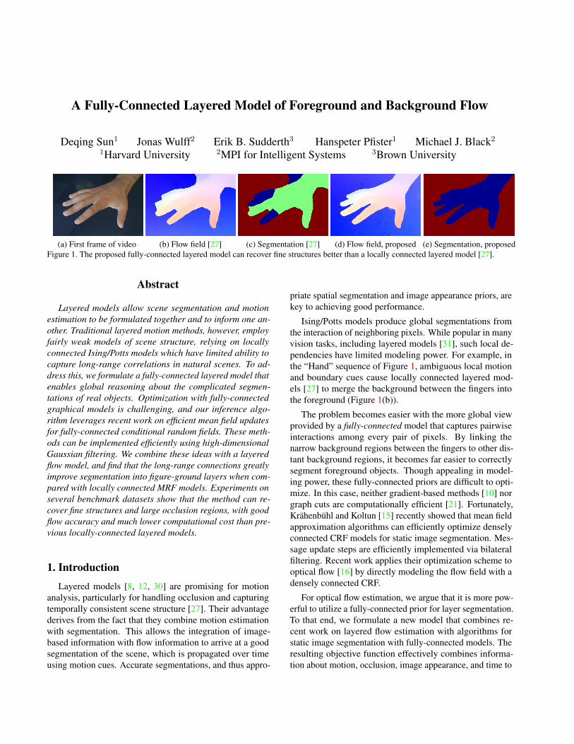
We use a binary mask gt to model the foreground supportat frame t. Pixels that are not visible in the foregroundbelong to the background layer. As shown in Figure 2, wemodel the binary mask spatially as a fully connected CRFand define the spatial energy term

Espace(gt)=∑p

∑q 6=p

wpqδ(gpt 6=gqt ), (2)

where a pixel is fully connected to all other pixels at thecurrent frame, δ(x) is 1 if x is true and 0 otherwise, and theweight wpq is defined as

wpq = ηG1(I

pt −I

qt , p−q)+(1−η)G2(p−q) = (3)

η exp

{−||I

pt −I

qt ||2

σ2I

− ||p−q||2

σ2s

}+(1−η) exp

{−||p−q||

2

σ2s′

},

where σI , σs, and σs′ are the standard deviations for theGaussian kernels, and η ∈ [0, 1] weights their relative impor-tance. The first (color) term encourages pixels with similarcolors, at moderate distances, to lie within the same layer.The second (spatial) term discourages small, isolated regions.Such small regions produce distracting segmentation arti-facts [15]. For our layered flow model, they further lead toinaccurate flow estimates; removing these isolated regionssignificantly reduces outliers in our final results.

The binary layer support masks evolve over time accord-

Figure 2. Spatial-temporal neighborhood structure for the binarymask defining foreground layer support. The center pixel (red) isspatially fully connected to all other pixels at the current frame. Thecenter pixel is also temporally connected to two temporal neighbors(green), as determined by the foreground and background flowvectors. The pair of temporal neighbors are only shown for the nextframe; the previous is omitted for clarity.

ing to the flow field of the foreground layer,

Etime(gt,gt+1,ut1,vt1) =∑

(p,q)∈Et1

δ(gpt 6=gqt+1), (4)

where Et1 = {(p, q) : q = p + (upt1, vpt1)} contains all

temporal neighbors linked by the foreground flow field. Asdiscussed in more detail in Sec. 3.2, we handle subpixelmotion by bilinear interpolation of the temporal neighbors.

The layer support mask provides a segmentation of thevideo sequence: a pixel p belongs to the foreground layerif gpt = 1, and to the background otherwise. We can thenreason about occlusions and modulate the data matchingterm accordingly, so that at frame t we have

Edata(gt,gt+1,ut,vt) =

2∑k=1

∑(p,q)∈Etk

φkdata(gpt , g

qt+1), (5)

where the negative log-likelihoods for the two layers are

φ1data(gpt , g

qt+1) =

(ρD(Ipt −I

qt )−λD

)gpt g

qt+1, (6)

φ2data(gpt , g

qt+1) =

(ρD(Ipt −I

qt )−λD

)gpt g

qt+1. (7)

Here, ρD(·) is a robust penalty and g = 1−g. The foregroundterm is only “on” when a pixel and its successor at the nextframe are both visible, gpt = gqt+1 = 1. The background termis active when gpt = gqt+1 = 0. The occlusion penalty λD >0 can be derived by assigning a uniform outlier distribution tooccluded (unmatched) pixels [26]. Note that occluded statesare less likely than flow vectors whose robust matching costsare smaller than λD.

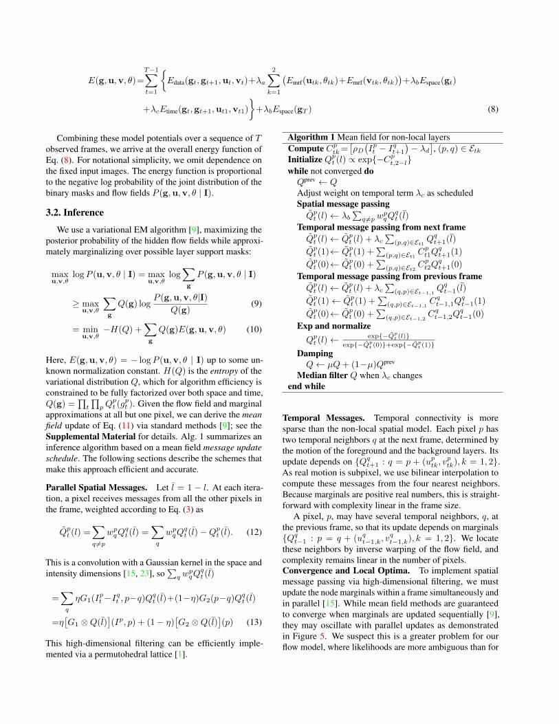
E(g,u,v, θ)=

T−1∑t=1

{Edata(gt,gt+1,ut,vt)+λa

2∑k=1

(Emrf(utk, θtk)+Emrf(vtk, θtk)

)+λbEspace(gt)

+λcEtime(gt,gt+1,ut1,vt1)

}+λbEspace(gT ) (8)

Combining these model potentials over a sequence of Tobserved frames, we arrive at the overall energy function ofEq. (8). For notational simplicity, we omit dependence onthe fixed input images. The energy function is proportionalto the negative log probability of the joint distribution of thebinary masks and flow fields P (g,u,v, θ | I).

3.2. Inference

We use a variational EM algorithm [9], maximizing theposterior probability of the hidden flow fields while approxi-mately marginalizing over possible layer support masks:

maxu,v,θ

logP (u,v, θ | I) = maxu,v,θ

log∑g

P (g,u,v, θ | I)

≥ maxu,v,θ

∑g

Q(g) logP (g,u,v, θ|I)

Q(g)(9)

= minu,v,θ

−H(Q) +∑g

Q(g)E(g,u,v, θ) (10)

Here, E(g,u,v, θ) = − logP (u,v, θ | I) up to some un-known normalization constant. H(Q) is the entropy of thevariational distribution Q, which for algorithm efficiency isconstrained to be fully factorized over both space and time,Q(g) =

∏t

∏pQ

pt (g

pt ). Given the flow field and marginal

approximations at all but one pixel, we can derive the meanfield update of Eq. (11) via standard methods [9]; see theSupplemental Material for details. Alg. 1 summarizes aninference algorithm based on a mean field message updateschedule. The following sections describe the schemes thatmake this approach efficient and accurate.

Parallel Spatial Messages. Let l = 1 − l. At each itera-tion, a pixel receives messages from all the other pixels inthe frame, weighted according to Eq. (3) as

Qpt (l) =∑q 6=p

wpqQqt (l) =

∑q

wpqQqt (l)−Q

pt (l). (12)

This is a convolution with a Gaussian kernel in the space andintensity dimensions [15, 23], so

∑q w

pqQ

qt (l)

=∑q

ηG1(Ipt −Iqt , p−q)Q

qt (l)+(1−η)G2(p−q)Qqt (l)

=η[G1 ⊗Q(l)

](Ip, p) + (1− η)

[G2 ⊗Q(l)

](p) (13)

This high-dimensional filtering can be efficiently imple-mented via a permutohedral lattice [1].

Algorithm 1 Mean field for non-local layersCompute Cptk=

[ρD(Ipt − I

qt+1

)− λd

], (p, q) ∈ Etk

Initialize Qpt (l) ∝ exp{−Cpt,2−l}while not converged doQprev ← QAdjust weight on temporal term λc as scheduledSpatial message passingQpt (l)← λb

∑q 6=p w

pqQ

qt (l)

Temporal message passing from next frameQpt (l)← Qpt (l) + λc

∑(p,q)∈Et1 Q

qt+1(l)

Qpt (1)← Qpt (1) +∑

(p,q)∈Et1 Cpt1Q

qt+1(1)

Qpt (0)← Qpt (0) +∑

(p,q)∈Et2 Cpt2Q

qt+1(0)

Temporal message passing from previous frameQpt (l)← Qpt (l) + λc

∑(q,p)∈Et−1,1

Qqt−1(l)

Qpt (1)← Qpt (1) +∑

(q,p)∈Et−1,1Cqt−1,1Q

qt−1(1)

Qpt (0)← Qpt (0) +∑

(q,p)∈Et−1,2Cqt−1,2Q

qt−1(0)

Exp and normalizeQpt (l)←

exp{−Qpt (l)}

exp{−Qpt (0)}+exp{−Qp

t (1)}DampingQ← µQ+ (1−µ)Qprev

Median filter Q when λc changesend while

Temporal Messages. Temporal connectivity is moresparse than the non-local spatial model. Each pixel p hastwo temporal neighbors q at the next frame, determined bythe motion of the foreground and the background layers. Itsupdate depends on {Qqt+1 : q = p + (uptk, v

ptk), k = 1, 2}.

As real motion is subpixel, we use bilinear interpolation tocompute these messages from the four nearest neighbors.Because marginals are positive real numbers, this is straight-forward with complexity linear in the frame size.

A pixel, p, may have several temporal neighbors, q, atthe previous frame, so that its update depends on marginals{Qqt−1 : p = q + (uqt−1,k, v

qt−1,k), k = 1, 2}. We locate

these neighbors by inverse warping of the flow field, andcomplexity remains linear in the number of pixels.Convergence and Local Optima. To implement spatialmessage passing via high-dimensional filtering, we mustupdate the node marginals within a frame simultaneously andin parallel [15]. While mean field methods are guaranteedto converge when marginals are updated sequentially [9],they may oscillate with parallel updates as demonstratedin Figure 5. We suspect this is a greater problem for ourflow model, where likelihoods are more ambiguous than for

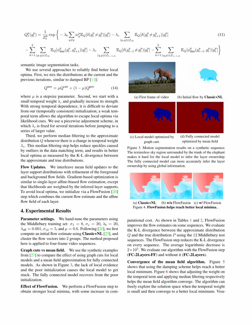
Qpt (gpt ) =

1

Zptexp

{− λb

∑q 6=p

wpqEQ[δ(gpt 6=gqt )|gpt ]− λc

∑(p,q)∈Etk

EQ[δ(gpt 6=gqt+1)|gpt ] (11)

−2∑k=1

∑(p,q)∈Etk

EQ[φkdata(gpt , g

qt+1)|gpt ]− λc

∑(q,p)∈Et−1,k

EQ[δ(gqt−1 6=gpt )|gpt ]−2∑k=1

∑(q,p)∈Et−1,k

EQ[φkdata(gqt−1, g

pt )|gpt ]

}

semantic image segmentation tasks.We use several approaches to reliably find better local

optima. First, we mix the distributions at the current and theprevious iterations, similar to damped BP [11]:

Qnew = µQcurr + (1− µ)Qprev (14)

where µ is a stepsize parameter. Second, we start with asmall temporal weight λc and gradually increase its strength.With strong temporal dependence, it is difficult to deviatefrom our (temporally consistent) initialization; a weak tem-poral term allows the algorithm to escape local optima vialikelihood cues. We use a piecewise adjustment scheme, inwhich λc is fixed for several iterations before jumping to aseries of larger value.

Third, we perform median filtering to the approximatedistributionQ whenever there is a change in temporal weightλc. This median filtering step helps reduce speckles causedby outliers in the data matching term, and results in betterlocal optima as measured by the K-L divergence betweenthe approximate and true distributions.

Flow Updates. We interleave mean field updates to thelayer support distributions with refinement of the foregroundand background flow fields. Gradient-based optimization issimilar to single-layer affine-biased flow estimation, exceptthat likelihoods are weighted by the inferred layer supports.To avoid local optima, we initialize via a FlowFusion [20]step which combines the current flow estimate and the affineflow field of each layer.

4. Experimental ResultsParameter settings. We hand-tune the parameters usingthe Middlebury training set: σI = 8, σs = 20, λb = 20,λaff = 0.001, σs2 = 5, and µ = 0.6. Following [26], we firstcompute an initial flow estimate using Classic+NL [25], andcluster the flow vectors into 2 groups. The method proposedhere is applied to four-frame video sequences.

Graph cuts vs mean field. We use the synthetic examplesfrom [27] to compare the effect of using graph cuts for localmodels and a mean field approximation for fully connectedmodels. As shown in Figure 3, the lack of local evidenceand the poor initialization causes the local model to getstuck. The fully connected model recovers from the poorinitialization.

Effect of FlowFusion. We perform a FlowFusion step toobtain stronger local minima, with some increase in com-

(a) First frame of video (b) Initial flow by Classic+NL

(c) Local model optimized bygraph cuts

(d) Fully connected modeloptimized by mean field

Figure 3. Motion segmentation results on a synthetic sequence.The textureless sky region surrounded by the trunk of the elephantmakes it hard for the local model to infer the layer ownership.The fully connected model can more accurately infer the layerownership by using global information.

(a) Classic+NL (b) w/o FlowFusion (c) w/ FlowFusionFigure 4. FlowFusion helps reach better local minima. .

putational cost. As shown in Tables 1 and 2, FlowFusionimproves the flow estimates on some sequences. We evaluatethe K-L divergence between the approximate distributionQ and the true distribution P using the 12 Middlebury testsequences. The FlowFusion step reduces the K-L divergenceon every sequence. The average logarithmic decrease is2 ∗ 105. We evaluate our algorithm with the FlowFusion step(FC-2Layers-FF) and without it (FC-2Layers).

Convergence of the mean field algorithm. Figure 5shows that using the damping scheme helps reach a betterlocal minimum. Figure 6 shows that adjusting the weight onthe temporal term and applying median filtering respectivelyhelps the mean field algorithm converge. The algorithm canfreely explore the solution space when the temporal weightis small and then converge to a better local minimum. Visu-

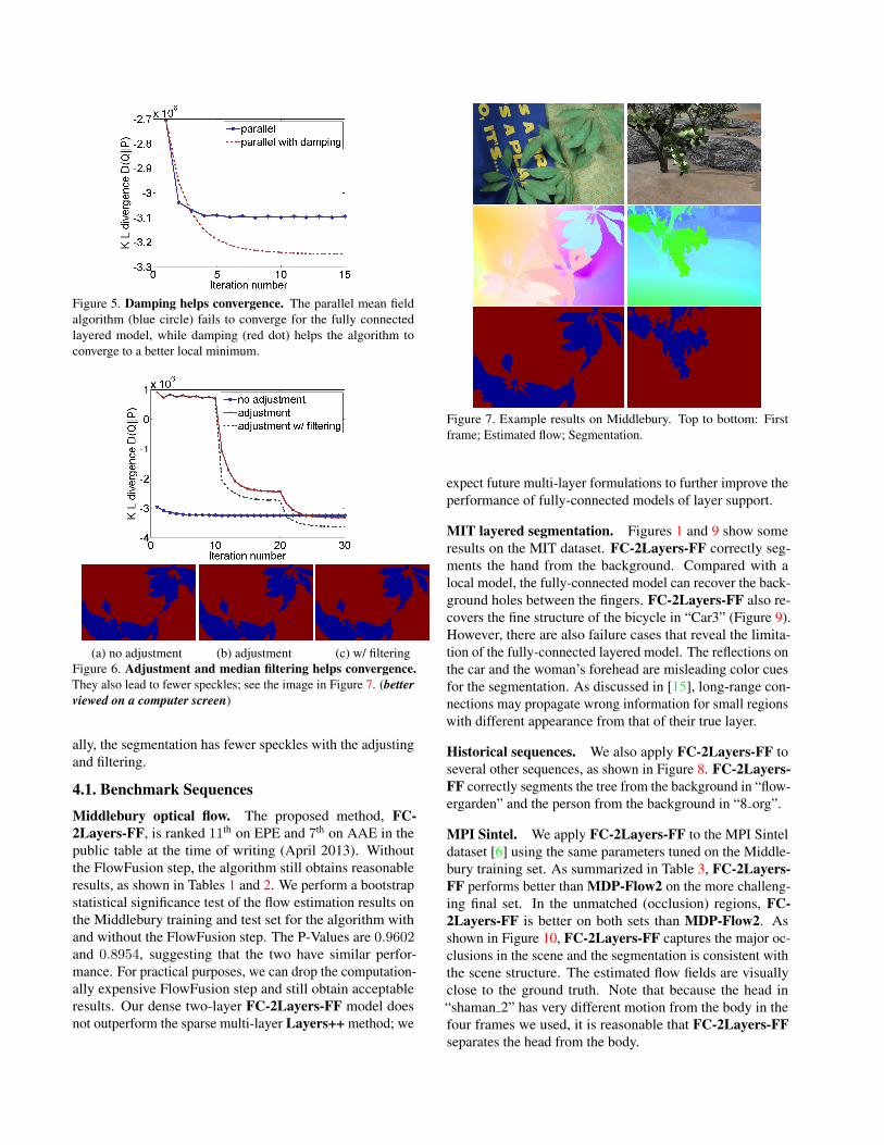
Figure 5. Damping helps convergence. The parallel mean fieldalgorithm (blue circle) fails to converge for the fully connectedlayered model, while damping (red dot) helps the algorithm toconverge to a better local minimum.

(a) no adjustment (b) adjustment (c) w/ filteringFigure 6. Adjustment and median filtering helps convergence.They also lead to fewer speckles; see the image in Figure 7. (betterviewed on a computer screen)

ally, the segmentation has fewer speckles with the adjustingand filtering.

4.1. Benchmark Sequences

Middlebury optical flow. The proposed method, FC-2Layers-FF, is ranked 11th on EPE and 7th on AAE in thepublic table at the time of writing (April 2013). Withoutthe FlowFusion step, the algorithm still obtains reasonableresults, as shown in Tables 1 and 2. We perform a bootstrapstatistical significance test of the flow estimation results onthe Middlebury training and test set for the algorithm withand without the FlowFusion step. The P-Values are 0.9602and 0.8954, suggesting that the two have similar perfor-mance. For practical purposes, we can drop the computation-ally expensive FlowFusion step and still obtain acceptableresults. Our dense two-layer FC-2Layers-FF model doesnot outperform the sparse multi-layer Layers++ method; we

Figure 7. Example results on Middlebury. Top to bottom: Firstframe; Estimated flow; Segmentation.

expect future multi-layer formulations to further improve theperformance of fully-connected models of layer support.

MIT layered segmentation. Figures 1 and 9 show someresults on the MIT dataset. FC-2Layers-FF correctly seg-ments the hand from the background. Compared with alocal model, the fully-connected model can recover the back-ground holes between the fingers. FC-2Layers-FF also re-covers the fine structure of the bicycle in “Car3” (Figure 9).However, there are also failure cases that reveal the limita-tion of the fully-connected layered model. The reflections onthe car and the woman’s forehead are misleading color cuesfor the segmentation. As discussed in [15], long-range con-nections may propagate wrong information for small regionswith different appearance from that of their true layer.

Historical sequences. We also apply FC-2Layers-FF toseveral other sequences, as shown in Figure 8. FC-2Layers-FF correctly segments the tree from the background in “flow-ergarden” and the person from the background in “8 org”.

MPI Sintel. We apply FC-2Layers-FF to the MPI Sinteldataset [6] using the same parameters tuned on the Middle-bury training set. As summarized in Table 3, FC-2Layers-FF performs better than MDP-Flow2 on the more challeng-ing final set. In the unmatched (occlusion) regions, FC-2Layers-FF is better on both sets than MDP-Flow2. Asshown in Figure 10, FC-2Layers-FF captures the major oc-clusions in the scene and the segmentation is consistent withthe scene structure. The estimated flow fields are visuallyclose to the ground truth. Note that because the head in“shaman 2” has very different motion from the body in thefour frames we used, it is reasonable that FC-2Layers-FFseparates the head from the body.

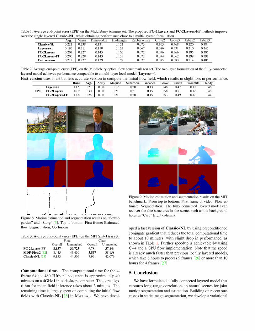
Table 1. Average end-point error (EPE) on the Middlebury training set. The proposed FC-2Layers and FC-2Layers-FF methods improveover the single layered Classic+NL, while obtaining performance close to a multi-layered formulation.

Avg. Venus Dimetrodon Hydrangea RubberWhale Grove2 Grove3 Urban2 Urban3Classic+NL 0.221 0.238 0.131 0.152 0.073 0.103 0.468 0.220 0.384Layers++ 0.195 0.211 0.150 0.161 0.067 0.086 0.331 0.210 0.345FC-2Layers 0.207 0.227 0.145 0.160 0.072 0.096 0.366 0.195 0.395FC-2Layers-FF 0.205 0.228 0.143 0.155 0.072 0.094 0.362 0.199 0.391Fast version 0.212 0.227 0.139 0.159 0.077 0.095 0.383 0.214 0.405

Table 2. Average end-point error (EPE) on the Middlebury optical flow benchmark test set. The two-layer formulation of the fully-connectedlayered model achieves performance comparable to a multi-layer local model (Layers++).Fast version uses a fast but less accurate version to compute the initial flow field, which results in slight loss in performance.

Rank Avg. Army Mequon Schefflera Wooden Grove Urban Yosemite Teddy

EPELayers++ 11.5 0.27 0.08 0.19 0.20 0.13 0.48 0.47 0.15 0.46FC-2Layers 16.9 0.30 0.08 0.21 0.21 0.15 0.58 0.51 0.16 0.48FC-2Layers-FF 13.8 0.28 0.08 0.21 0.20 0.15 0.53 0.49 0.16 0.44

Figure 8. Motion estimation and segmentation results on “flower-garden” and “8 org” [3]. Top to bottom: First frame; Estimatedflow; Segmentation; Occlusions.

Table 3. Average end-point error (EPE) on the MPI Sintel test set.Final Clean

Overall Unmatched Overall UnmatchedFC-2Layers-FF 8.137 39.723 6.781 37.144MDP-Flow2 [32] 8.445 43.430 5.837 38.158Classic+NL [25] 9.153 44.509 7.961 42.079

Computational time. The computational time for the 4-frame 640 × 480 “Urban” sequence is approximately 40minutes on a 4GHz Linux desktop computer. The core algo-rithm for mean field inference takes about 5 minutes. Theremaining time is largely spent on computing the initial flowfields with Classic+NL [25] in MATLAB. We have devel-

Figure 9. Motion estimation and segmentation results on the MITbenchmark. From top to bottom: First frame of video; Flow es-timate; Segmentation. The fully connected layered model canrecover the fine structures in the scene, such as the backgroundholes in “Car3” (right column).

oped a fast version of Classic+NL by using preconditionedconjugate gradient that reduces the total computational timeto about 10 minutes, with slight drop in performance, asshown in Table 1. Further speedup is achievable by usingC++ and a GPU flow implementation. Note that the speedis already much faster than previous locally layered models,which take 5 hours to process 2 frames [26] or more than 10hours for 4 frames [27].

5. ConclusionWe have formulated a fully-connected layered model that

captures long-range correlations in natural scenes for jointmotion segmentation and estimation. Building on recent suc-cesses in static image segmentation, we develop a variational

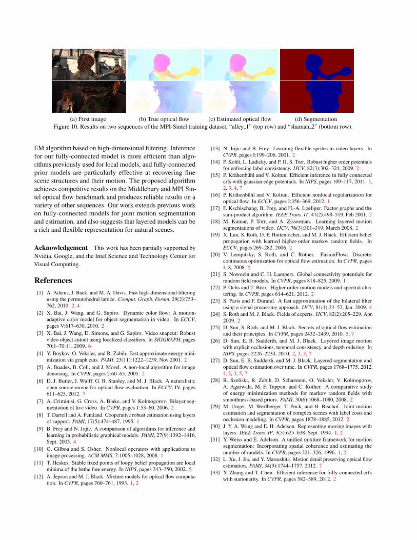
(a) First image (b) True optical flow (c) Estimated optical flow (d) SegmentationFigure 10. Results on two sequences of the MPI-Sintel training dataset, “alley 1” (top row) and “shaman 2” (bottom row).

EM algorithm based on high-dimensional filtering. Inferencefor our fully-connected model is more efficient than algo-rithms previously used for local models, and fully-connectedprior models are particularly effective at recovering finescene structures and their motion. The proposed algorithmachieves competitive results on the Middlebury and MPI Sin-tel optical flow benchmark and produces reliable results on avariety of other sequences. Our work extends previous workon fully-connected models for joint motion segmentationand estimation, and also suggests that layered models can bea rich and flexible representation for natural scenes.

Acknowledgement This work has been partially supported byNvidia, Google, and the Intel Science and Technology Center forVisual Computing.

References[1] A. Adams, J. Baek, and M. A. Davis. Fast high-dimensional filtering

using the permutohedral lattice. Comput. Graph. Forum, 29(2):753–762, 2010. 2, 4

[2] X. Bai, J. Wang, and G. Sapiro. Dynamic color flow: A motion-adaptive color model for object segmentation in video. In ECCV,pages V:617–630, 2010. 2

[3] X. Bai, J. Wang, D. Simons, and G. Sapiro. Video snapcut: Robustvideo object cutout using localized classifiers. In SIGGRAPH, pages70:1–70:11, 2009. 6

[4] Y. Boykov, O. Veksler, and R. Zabih. Fast approximate energy mini-mization via graph cuts. PAMI, 23(11):1222–1239, Nov 2001. 2

[5] A. Buades, B. Coll, and J. Morel. A non-local algorithm for imagedenoising. In CVPR, pages 2:60–65, 2005. 2

[6] D. J. Butler, J. Wulff, G. B. Stanley, and M. J. Black. A naturalisticopen source movie for optical flow evaluation. In ECCV, IV, pages611–625, 2012. 7

[7] A. Criminisi, G. Cross, A. Blake, and V. Kolmogorov. Bilayer seg-mentation of live video. In CVPR, pages 1:53–60, 2006. 2

[8] T. Darrell and A. Pentland. Cooperative robust estimation using layersof support. PAMI, 17(5):474–487, 1995. 1

[9] B. Frey and N. Jojic. A comparison of algorithms for inference andlearning in probabilistic graphical models. PAMI, 27(9):1392–1416,Sept. 2005. 4

[10] G. Gilboa and S. Osher. Nonlocal operators with applications toimage processing. ACM MMS, 7:1005–1028, 2008. 1

[11] T. Heskes. Stable fixed points of loopy belief propagation are localminima of the bethe free energy. In NIPS, pages 343–350, 2002. 5

[12] A. Jepson and M. J. Black. Mixture models for optical flow computa-tion. In CVPR, pages 760–761, 1993. 1, 2

[13] N. Jojic and B. Frey. Learning flexible sprites in video layers. InCVPR, pages I:199–206, 2001. 2

[14] P. Kohli, L. Ladicky, and P. H. S. Torr. Robust higher order potentialsfor enforcing label consistency. IJCV, 82(3):302–324, 2009. 2

[15] P. Krahenbuhl and V. Koltun. Efficient inference in fully connectedcrfs with gaussian edge potentials. In NIPS, pages 109–117, 2011. 1,2, 3, 4, 7

[16] P. Krahenbuhl and V. Koltun. Efficient nonlocal regularization foroptical flow. In ECCV, pages I:356–369, 2012. 1

[17] F. Kschischang, B. Frey, and H.-A. Loeliger. Factor graphs and thesum-product algorithm. IEEE Trans. IT, 47(2):498–519, Feb 2001. 2

[18] M. Kumar, P. Torr, and A. Zisserman. Learning layered motionsegmentations of video. IJCV, 76(3):301–319, March 2008. 2

[19] X. Lan, S. Roth, D. P. Huttenlocher, and M. J. Black. Efficient beliefpropagation with learned higher-order markov random fields. InECCV, pages 269–282, 2006. 2

[20] V. Lempitsky, S. Roth, and C. Rother. FusionFlow: Discrete-continuous optimization for optical flow estimation. In CVPR, pages1–8, 2008. 5

[21] S. Nowozin and C. H. Lampert. Global connectivity potentials forrandom field models. In CVPR, pages 818–825, 2009. 1

[22] P. Ochs and T. Brox. Higher order motion models and spectral clus-tering. In CVPR, pages 614–621, 2012. 2

[23] S. Paris and F. Durand. A fast approximation of the bilateral filterusing a signal processing approach. IJCV, 81(1):24–52, Jan. 2009. 4

[24] S. Roth and M. J. Black. Fields of experts. IJCV, 82(2):205–229, Apr.2009. 2

[25] D. Sun, S. Roth, and M. J. Black. Secrets of optical flow estimationand their principles. In CVPR, pages 2432–2439, 2010. 5, 7

[26] D. Sun, E. B. Sudderth, and M. J. Black. Layered image motionwith explicit occlusions, temporal consistency, and depth ordering. InNIPS, pages 2226–2234, 2010. 2, 3, 5, 7

[27] D. Sun, E. B. Sudderth, and M. J. Black. Layered segmentation andoptical flow estimation over time. In CVPR, pages 1768–1775, 2012.1, 2, 3, 5, 7

[28] R. Szeliski, R. Zabih, D. Scharstein, O. Veksler, V. Kolmogorov,A. Agarwala, M. F. Tappen, and C. Rother. A comparative studyof energy minimization methods for markov random fields withsmoothness-based priors. PAMI, 30(6):1068–1080, 2008. 2

[29] M. Unger, M. Werlberger, T. Pock, and H. Bischof. Joint motionestimation and segmentation of complex scenes with label costs andocclusion modeling. In CVPR, pages 1878–1885, 2012. 2

[30] J. Y. A. Wang and E. H. Adelson. Representing moving images withlayers. IEEE Trans. IP, 3(5):625–638, Sept. 1994. 1, 2

[31] Y. Weiss and E. Adelson. A unified mixture framework for motionsegmentation: Incorporating spatial coherence and estimating thenumber of models. In CVPR, pages 321–326, 1996. 1, 2

[32] L. Xu, J. Jia, and Y. Matsushita. Motion detail preserving optical flowestimation. PAMI, 34(9):1744–1757, 2012. 7

[33] Y. Zhang and T. Chen. Efficient inference for fully-connected crfswith stationarity. In CVPR, pages 582–589, 2012. 2