Embed Size (px)
Citation preview
A FRACTAL VALUE RANDOM ITERATION ALGORITHM ANDFRACTAL HIERARCHY
MICHAEL BARNSLEY, JOHN HUTCHINSON, AND ÖRJAN STENFLO
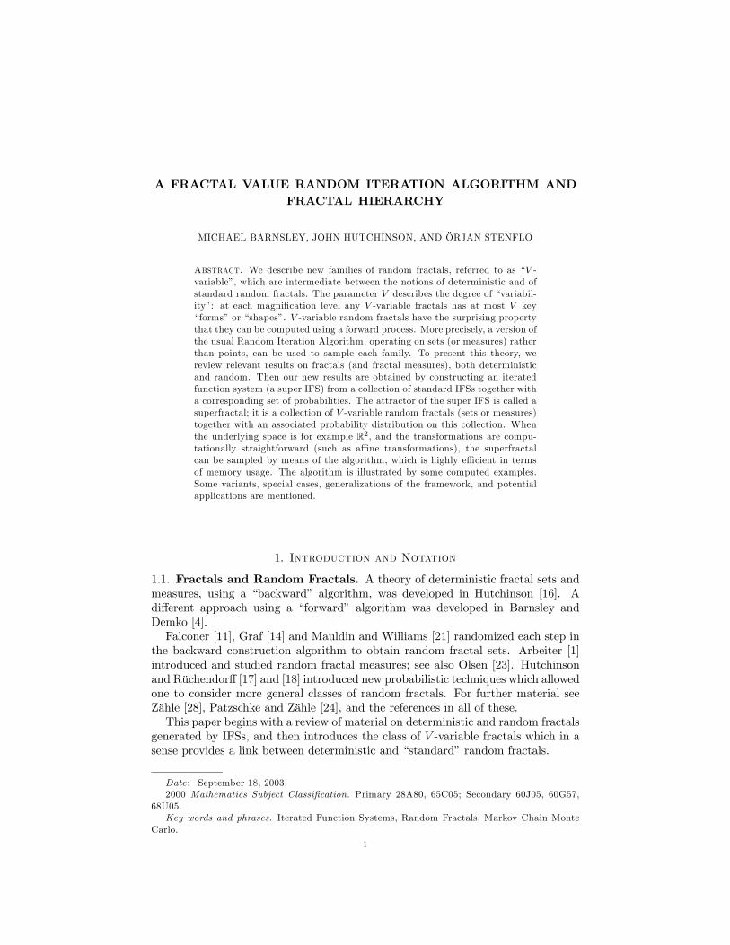
Abstract. We describe new families of random fractals, referred to as “V -variable”, which are intermediate between the notions of deterministic and ofstandard random fractals. The parameter V describes the degree of “variabil-ity”: at each magnification level any V -variable fractals has at most V key“forms” or “shapes”. V -variable random fractals have the surprising propertythat they can be computed using a forward process. More precisely, a version ofthe usual Random Iteration Algorithm, operating on sets (or measures) ratherthan points, can be used to sample each family. To present this theory, wereview relevant results on fractals (and fractal measures), both deterministicand random. Then our new results are obtained by constructing an iteratedfunction system (a super IFS) from a collection of standard IFSs together witha corresponding set of probabilities. The attractor of the super IFS is called asuperfractal; it is a collection of V -variable random fractals (sets or measures)together with an associated probability distribution on this collection. Whenthe underlying space is for example R2, and the transformations are compu-tationally straightforward (such as affine transformations), the superfractalcan be sampled by means of the algorithm, which is highly efficient in termsof memory usage. The algorithm is illustrated by some computed examples.Some variants, special cases, generalizations of the framework, and potentialapplications are mentioned.
1. Introduction and Notation
1.1. Fractals and Random Fractals. A theory of deterministic fractal sets andmeasures, using a “backward” algorithm, was developed in Hutchinson [16]. Adifferent approach using a “forward” algorithm was developed in Barnsley andDemko [4].Falconer [11], Graf [14] and Mauldin and Williams [21] randomized each step in
the backward construction algorithm to obtain random fractal sets. Arbeiter [1]introduced and studied random fractal measures; see also Olsen [23]. Hutchinsonand Rüchendorff [17] and [18] introduced new probabilistic techniques which allowedone to consider more general classes of random fractals. For further material seeZähle [28], Patzschke and Zähle [24], and the references in all of these.This paper begins with a review of material on deterministic and random fractals
generated by IFSs, and then introduces the class of V -variable fractals which in asense provides a link between deterministic and “standard” random fractals.
Date : September 18, 2003.2000 Mathematics Subject Classification. Primary 28A80, 65C05; Secondary 60J05, 60G57,
68U05.Key words and phrases. Iterated Function Systems, Random Fractals, Markov Chain Monte
Carlo.
1
2 MICHAEL BARNSLEY, JOHN HUTCHINSON, AND ÖRJAN STENFLO
Deterministic fractal sets and measures are defined as the attractors of certainiterated function systems (IFSs), as reviewed in Section 2. Approximations in prac-tical situations quite easily can be computed using the associated random iterationalgorithm. Random fractals are typically harder to compute because one has tofirst calculate lots of fine random detail at low levels, then one level at a time, buildup the higher levels.In this paper we restrict the class of random fractals to ones that we call random
V -variable fractals. Superfractals are sets of V -variable fractals. They can bedefined using a new type of IFS, in fact a “super” IFS made of a finite number Nof IFSs, and there is available a novel random iteration algorithm: each iterationproduces new sets, lying increasingly close to V-variable fractals belonging to thesuperfractal, and moving ergodically around the superfractal.Superfractals appear to be a new class of geometrical object, their elements ly-
ing somewhere between fractals generated by IFSs with finitely many maps, whichcorrespond to V = N = 1, and realizations of the most generic class of randomfractals, where the local structure around each of two distinct points are indepen-dent, corresponding to V = ∞. They seem to allow geometric modelling of somenatural objects, examples including realistic-looking leaves, clouds, and textures;and good approximations can be computed fast in elementary computer graphicsexamples. They are fascinating to watch, one after another, on a computer screen,diverse, yet ordered enough to suggest coherent natural phenomena and potentialapplications.Areas of potential applications include computer graphics and rapid simulation of
trajectories of stochastic processes The forward algorithm also enables rapid com-putation of good approximations to random (including “fully” random) processes,where previously there was no available efficient algorithm.
1.2. An Example. Here we give an illustration of an application of the theory inthis paper. By means of this example we introduce informally V-variable fractalsand superfractals. We also explain why we think these objects are of special interestand deserve attention.We start with two pairs of contractive affine transformations, f11 , f12 and
f21 , f22 , where fnm : ¤ → ¤ with ¤ := [0, 1] × [0, 1] ⊂ R2. We use two pairsof screens, where each screen corresponds to a copy of ¤ and represents for exam-ple a computer monitor. We designate one pair of screens to be the Input Screens,denoted by (¤1,¤2). The other pair of screens is designated to be the OutputScreens, denoted by (¤10 ,¤20).Initialize by placing an image on each of the Input Screens, as illustrated in
Figure 2, and clearing both of the Output Screens. We construct an image on eachof the two Output Screens as follows.(i) Pick randomly one of the pairs of functions f11 , f12 or f21 , f22 , sayfn11 , fn12 .
Apply fn11 to one of the images on ¤1 or ¤2, selected randomly, to make an imageon ¤10 . Then apply fn12 to one of the images on ¤1 or ¤2, also selected randomly,and overlay the resulting image I on the image now already on ¤10 . (For example,if black-and-white images are used, simply take the union of the black region of Iwith the black region on ¤10 , and put the result back onto ¤10 .)(ii) Again pick randomly one of the pairs of functions f11 , f12 or f21 , f22 , say
fn21 , fn22 . Apply fn21 to one of the images on ¤1, or ¤2, selected randomly, tomake an image on ¤20 . Also apply fn22 to one of the images on ¤1, or ¤2, also
RANDOM IFSS 3
0.25 0.75 10.50
0.25
0.5
0.75
1
B
CA
D
B1 B2
B4B3
y
x
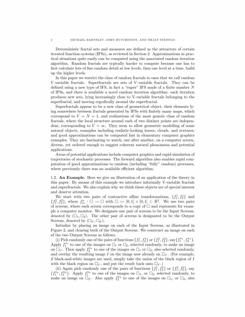
Figure 1. Triangles used to define the four transformationsf11 , f
12 , f
21 , and f22 .
selected randomly, and overlay the resulting image on the image now already on¤20 .(iii) Switch Input and Output, clear the new Output Screens, and repeat steps
(i), and (ii).(iv) Repeat step (iii) many times, to allow the system to settle into its “stationary
state”.What kinds of images do we see on the successive pairs of screens, and what are
they like in the “stationary state”? What does the theory developed in this papertell us about such situations?As a specific example, let us choose
(1.1) f11 (x, y) = (1
2x− 3
8y +
5
16,1
2x+
3
8y +
3
16),
(1.2) f12 (x, y) = (1
2x+
3
8y +
3
16,−12x+
3
8y +
11
16),
f21 (x, y) = (1
2x− 3
8y +
5
16,−12x− 3
8y +
13
16),
(1.3) f22 (x, y) = (1
2x+
3
8y +
3
16,1
2x− 3
8y +
5
16).
We describe how these transformations act on the triangle ABC in the diamondABCD, where A = (14 ,
12), B = (12 ,
34), C = ( 34 ,
12), and D = (12 ,
14). Let B1 =
( 932 ,2332), B2 = (
2332 ,
2332 ), B3 = (
932 ,
932), and B4 = (
2332 ,
2332). See Figure 1. Then we
havef11 (A) = A, f11 (B) = B1, f11 (C) = B;
f12 (A) = B, f12 (B) = B2, f12 (C) = C;
4 MICHAEL BARNSLEY, JOHN HUTCHINSON, AND ÖRJAN STENFLO
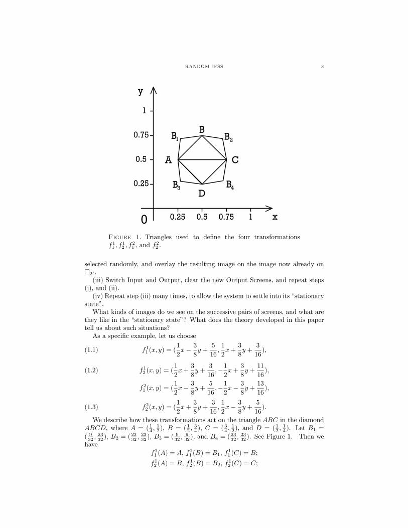
Figure 2. An initial image of a jumping fish on each of the twoscreens ¤1 and ¤2.
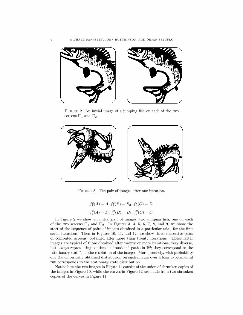
Figure 3. The pair of images after one iteration.
f21 (A) = A, f21 (B) = B3, f21 (C) = D;
f22 (A) = D, f22 (B) = B4, f22 (C) = C.
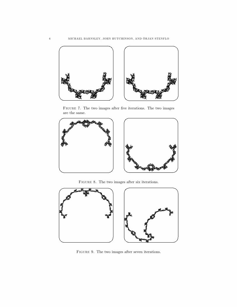
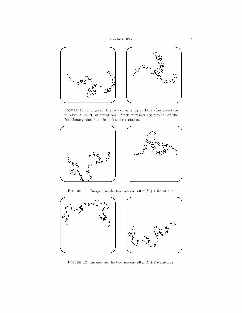
In Figure 2 we show an initial pair of images, two jumping fish, one on eachof the two screens ¤1 and ¤2. In Figures 3, 4, 5, 6, 7, 8, and 9, we show thestart of the sequence of pairs of images obtained in a particular trial, for the firstseven iterations. Then in Figures 10, 11, and 12, we show three successive pairsof computed screens, obtained after more than twenty iterations. These latterimages are typical of those obtained after twenty or more iterations, very diverse,but always representing continuous “random” paths in R2; they correspond to the“stationary state”, at the resolution of the images. More precisely, with probabilityone the empirically obtained distribution on such images over a long experimentalrun corresponds to the stationary state distribution.Notice how the two images in Figure 11 consist of the union of shrunken copies of
the images in Figure 10, while the curves in Figure 12 are made from two shrunkencopies of the curves in Figure 11.
RANDOM IFSS 5
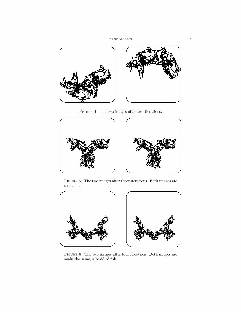
Figure 4. The two images after two iterations.
Figure 5. The two images after three iterations. Both images arethe same.
Figure 6. The two images after four iterations. Both images areagain the same, a braid of fish.
6 MICHAEL BARNSLEY, JOHN HUTCHINSON, AND ÖRJAN STENFLO
Figure 7. The two images after five iterations. The two imagesare the same.
Figure 8. The two images after six iterations.
Figure 9. The two images after seven iterations.
RANDOM IFSS 7
Figure 10. Images on the two screens ¤1 and ¤2 after a certainnumber L > 20 of iterations. Such pictures are typical of the"stationary state" at the printed resolution.
Figure 11. Images on the two screens after L+ 1 iterations.
Figure 12. Images on the two screens after L+ 2 iterations.
8 MICHAEL BARNSLEY, JOHN HUTCHINSON, AND ÖRJAN STENFLO
This example illustrates some typical features of the theory in this paper. (i) Newimages are generated, one per iteration per screen. (ii) After sufficient iterationsfor the system to have settled into its “stationary state”, each image looks like afinite resolution rendering of a fractal set that typically changes from one iterationto the next; each fractal belongs to the same family, in the present case a familyof continuous curves. (iii) In fact, it follows from the theory that the pictures inthis example correspond to curves with this property: for any > 0 the curve isthe union of “little” curves, ones such that the distance apart of any two pointsis no more than , each of which is an affine transformation of one of at mosttwo continuous closed paths in R2. (iv) We will show that the successive images,or rather the abstract objects they represent, eventually all lie arbitrarily close toan object called a superfractal. The superfractal is the attractor of a superIFSwhich induces a natural invariant probability measure on the superfractal. Theimages produced by the algorithm are distributed according to this measure. (v)The images produced in the “stationary state” are independent of the startingimages. For example, if the initial images in the example had been of a dot or aline instead of a fish, and the same sequence of random choices had been made,then the images produced in Figures 10, 11, and 12 would have been the same atthe printed resolution.One similarly obtains V-variable fractals and their properties using V , rather
than two, screens and otherwise proceeding similarly. In (iii) each of the sets ofdiameter at most is an affine transformation of at most V sets in R2, where thesesets again depend upon and the particular image.This example and the features just mentioned suggest that superfractals are of
interest because they provide a natural mathematical bridge between deterministicand random fractals, and because they may lead to practical applications in digitalimaging, special effects, computer graphics, as well as in the many other areas wherefractal geometric modelling is applied.
1.3. The structure of this paper. The main contents of this paper, while con-ceptually not very difficult, involves potentially elaborate notation because we dealwith iterated function systems (IFSs) made of IFSs, and probability measures onspaces of probability measures. So a material part of our effort has been towardsa simplified notation. Thus, below, we set out some notation and conventions thatwe use throughout.The core machinery that we use is basic IFS theory, as described in [16] and [4].
So in Section 2 we review relevant parts of this theory, using notation and organiza-tion that extends to and simplifies later material. To keep the structural ideas clear,we restrict attention to IFSs with strictly contractive transformations and constantprobabilities. Of particular relevance to this paper, we explain what is meant bythe random iteration algorithm. We illustrate the theorems with simple applica-tions to two-dimensional computer graphics, both to help with understanding andto draw attention to some issues related to discretization that apply a fortiori incomputations of V-variable fractals.We begin Section 3 with the definition of a superIFS, namely an IFS made of
IFSs. We then introduce associated trees, in particular labelled trees, the spaceof code trees Ω, and construction trees; then we review standard random fractalsusing the terminology of trees and superIFSs.
RANDOM IFSS 9
In Section 4 we study a special class of code trees, called V -variable trees,where V is an integer. What are these trees like? At each level they have atmost V distinct subtrees! In fact these trees are described with the aid of an IFSΩV ; ηa,Pa, a ∈ A where A is a finite index set, Pas are probabilities, and each ηa
is a contraction mapping from ΩV to itself. The IFS enables one to put a measureattractor on the set of V -variable trees, such that they can be sampled by meansof the random iteration algorithm. We describe the mappings ηa and composi-tions of them using certain finite doubly labelled trees. This, in turn, enables usto establish the convergence, as V → ∞, of the probability measure on the set ofV -variable trees, associated with the IFS and the random iteration algorithm, to acorresponding natural probability distribution on the space Ω.In Section 5 the discussion of trees in Section 4 is recapitulated twice over: the
same basic IFS theory is applied in two successively more elaborate settings, yieldingthe formal concepts of V-variable fractals and superfractals. More specifically, inSection 5.1, the superIFS is used to define an IFS of functions that map V -tuples ofcompact sets into V -tuples of compact sets; the attractor of this IFS is a set of V -tuples of compact sets; these compact sets are named V -variable fractals and the setof these V -variable fractals is named a superfractal. We show that these V -variablefractals can be sampled by means of the random iteration algorithm, adapted to thepresent setting; that they are distributed according to a certain stationary measureon the superfractal; and that this measure converges to a corresponding measureon the set of “fully” random fractals as V → ∞, in an appropriate metric. Wealso provide a continuous mapping from the set of V -variable trees to the set ofV -variable fractals, and characterize the V -variable fractals in terms of a propertythat we name “V -variability”. Section 5.2 follows the same lines as in Section5.1, except that here the superIFS is used to define an IFS that maps V -tuplesof measures to V -tuples of measures; this leads to the definition and properties ofV -variable fractal measures. In Section 5.3 we describe how to compute the fractaldimensions of V-variable fractals in certain cases and compare them, in a caseinvolving Sierpinski triangles, with the fractal dimensions of deterministic fractals,“fully” random fractals, and “homogeneous” random fractals that correspond toV = 1 and are a special case of a type of random fractal investigated by Hamblyand others [15], [2], [19], [27].In Section 6 we describe some potential applications of the theory including new
types of space-filling curves for digital imaging, geometric modelling and texturerendering in digital content creation, and random fractal interpolation for computeraided design systems. In Section 7 we discuss generalizations and extensions of thetheory, areas of ongoing research, and connections to the work of others.
1.4. Some Notation. We use notation and terminology consistent with [4].Throughout we reserve the symbols M , N , and V for positive integers. We will
use the variables m ∈ 1, 2, ...,M, n ∈ 1, 2, ..., N, and v ∈ 1, 2, ..., V .Throughout we use an underlying metric space (X, dX) which is assumed to be
compact unless otherwise stated. We write XV to denote the compact metric space
X×X× ...× X| z V TIMES
.
with metric
d(x, y) = dXV (x, y) = max dX(xv, yv) | v = 1, 2, ..., V , ∀x, y ∈ XV ,
10 MICHAEL BARNSLEY, JOHN HUTCHINSON, AND ÖRJAN STENFLO
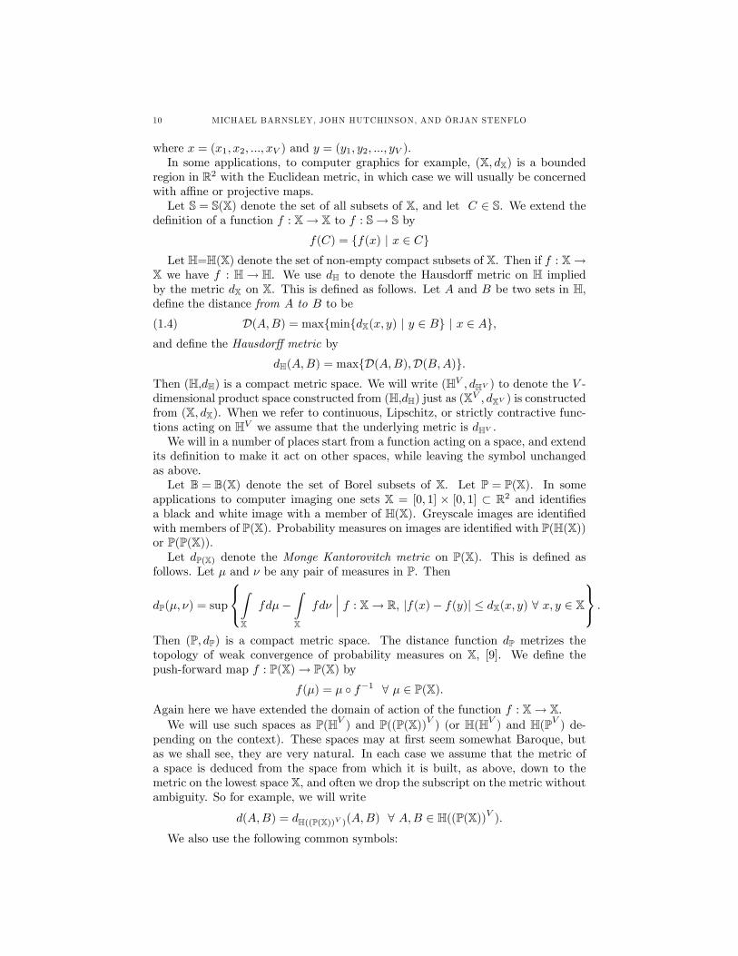
where x = (x1, x2, ..., xV ) and y = (y1, y2, ..., yV ).In some applications, to computer graphics for example, (X, dX) is a bounded
region in R2 with the Euclidean metric, in which case we will usually be concernedwith affine or projective maps.Let S = S(X) denote the set of all subsets of X, and let C ∈ S. We extend the
definition of a function f : X→ X to f : S→ S byf(C) = f(x) | x ∈ C
Let H=H(X) denote the set of non-empty compact subsets of X. Then if f : X→X we have f : H→ H. We use dH to denote the Hausdorff metric on H impliedby the metric dX on X. This is defined as follows. Let A and B be two sets in H,define the distance from A to B to be
(1.4) D(A,B) = maxmindX(x, y) | y ∈ B | x ∈ A,and define the Hausdorff metric by
dH(A,B) = maxD(A,B),D(B,A).Then (H,dH) is a compact metric space. We will write (HV , dHV ) to denote the V -dimensional product space constructed from (H,dH) just as (XV , dXV ) is constructedfrom (X, dX). When we refer to continuous, Lipschitz, or strictly contractive func-tions acting on HV we assume that the underlying metric is dHV .We will in a number of places start from a function acting on a space, and extend
its definition to make it act on other spaces, while leaving the symbol unchangedas above.Let B = B(X) denote the set of Borel subsets of X. Let P = P(X). In some
applications to computer imaging one sets X = [0, 1] × [0, 1] ⊂ R2 and identifiesa black and white image with a member of H(X). Greyscale images are identifiedwith members of P(X). Probability measures on images are identified with P(H(X))or P(P(X)).Let dP(X) denote the Monge Kantorovitch metric on P(X). This is defined as
follows. Let µ and ν be any pair of measures in P. Then
dP(µ, ν) = sup
ZX
fdµ−ZX
fdν¯f : X→ R, |f(x)− f(y)| ≤ dX(x, y) ∀ x, y ∈ X
.
Then (P, dP) is a compact metric space. The distance function dP metrizes thetopology of weak convergence of probability measures on X, [9]. We define thepush-forward map f : P(X)→ P(X) by
f(µ) = µ f−1 ∀ µ ∈ P(X).Again here we have extended the domain of action of the function f : X→ X.We will use such spaces as P(HV
) and P((P(X))V ) (or H(HV) and H(PV ) de-
pending on the context). These spaces may at first seem somewhat Baroque, butas we shall see, they are very natural. In each case we assume that the metric ofa space is deduced from the space from which it is built, as above, down to themetric on the lowest space X, and often we drop the subscript on the metric withoutambiguity. So for example, we will write
d(A,B) = dH((P(X))V )(A,B) ∀ A,B ∈ H((P(X))V ).We also use the following common symbols:
RANDOM IFSS 11
N = 1, 2, 3, ..., Z = ...− 2,−1, 0, 1, 2, ..., and Z+= 0, 1, 2, ....When S is a set, |S| denotes the number of elements of S.
2. Iterated Function Systems
2.1. Definitions and Basic Results. In this section we review relevant infor-mation about IFSs. To clarify the essential ideas we consider the case where allmappings are contractive, but indicate in Section 5 how these ideas can be gener-alized. The machinery and ideas introduced here are applied repeatedly later on inmore elaborate settings.Let
(2.1) F = X; f1, f2, ..., fM ; p1, p2, ..., pMdenote an IFS with probabilities. The functions fm : X→ X are contraction map-pings with fixed Lipschitz constant 0 ≤ l < 1; that is
d(fm(x), fm(y)) ≤ l · d(x, y) ∀x, y ∈ X,∀m ∈ 1, 2, ...,M.The pm’s are probabilities, with
MXm=1
pm = 1, pm ≥ 0 ∀m.
We define mappings F : H(X)→ H(X) and F : P(X)→ P(X) by
F (K) =M[m=1
fm(K) ∀K ∈ H,
and
F (µ) =MXm=1
pmfm(µ) ∀µ ∈ P.
In the latter case note that the weighted sum of probability measures is again aprobability measure.
Theorem 1. [16]The mappings F : H(X) → H(X) and F : P(X) → P(X) are bothcontractions with factor 0 ≤ l < 1. That is,
d(F (K), F (L)) ≤ l · d(K,L) ∀ K,L ∈ H(X),and
d(F (µ), F (ν)) ≤ l · d(µ, ν) ∀ µ, ν ∈ P(X).As a consequence, there exists a unique nonempty compact set A ∈ H(X) such that
F (A) = A,
and a unique measure µ ∈ P(X) such thatF (µ) = µ.
The support of µ is contained in, or equal to A, with equality when all of theprobabilities pm are strictly positive.
Definition 1. The set A in Theorem 1 is called the set attractor of the IFS F , andthe measure µ is called the measure attractor of F .
12 MICHAEL BARNSLEY, JOHN HUTCHINSON, AND ÖRJAN STENFLO
We will use the term attractor of an IFS to mean either the set attractor or themeasure attractor. We will also refer informally to the set attractor of an IFS as afractal and to its measure attractor as a fractal measure, and to either as a fractal.Furthermore, we say that the set attractor of an IFS is a deterministic fractal. Thisis in distinction to random fractals, and in particular to V -variable random fractalswhich are the main goal of this paper.There are two main types of algorithms for the practical computation of attrac-
tors of IFS that we term deterministic algorithms and random iteration algorithms,also known as backward and forward algorithms, c.f. [8]. These terms should notbe confused with the type of fractal that is computed by means of the algorithm.Both deterministic and random iteration algorithms may be used to compute deter-ministic fractals, and as we discuss later, a similar remark applies to our V -variablefractals.Deterministic algorithms are based on the following:
Corollary 1. Let A0 ∈ H(X), or µ0 ∈ P(X), and define recursivelyAk = F (Ak−1), or µk = F (µk−1), ∀k ∈ N,
respectively; then
(2.2) limk→∞
Ak = A, or limk→∞
µk = µ,
respectively. The rate of convergence is geometrical; for example,
d(Ak, A) ≤ lk · d(A0, A) ∀k ∈ N.In practical applications to two-dimensional computer graphics, the transfor-
mations and the spaces upon which they act must be discretized. The precisebehaviour of computed sequences of approximations to an attractor of an IFS de-pends on the details of the implementation and is generally quite complicated; forexample, the discrete IFS may have multiple attractors, see [25], Chapter 4. Thefollowing example gives the flavour of such applications.
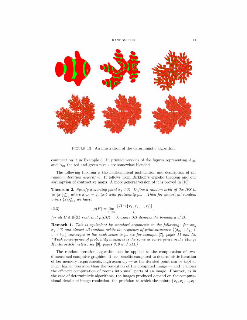
Example 1. In Figure 13 we illustrate a practical deterministic algorithm, basedon the first formula in Equation (2.2) starting from a simple IFS on the unit square¤ ⊂ R2. The IFS is F = ¤; f11 , f12 , f22 ; 0.36, 0.28, 0.36 where the transformationsare defined in Equations (1.1), (1.2), and (1.3). The successive images, from leftto right, from top to bottom, represent A0, A2, A5, A7, A20, and A21. In thelast two images, the sequence appears to have converged at the printed resolutionto representations of the set attractor. Note however that the initial image ispartitioned into two subsets corresponding to the colours red and green. Eachsuccessive computed image is made of pixels belonging to a discrete model for ¤and consists of red pixels and green pixels. Each pixel corresponds to a set of pointsin R2. But for the purposes of computation only one point corresponding to eachpixel is used. When both a point in a red pixel and point in a green pixel belongingto say An are mapped under F to points in the same pixel in An+1 a choice has tobe made about which colour, red or green, to make the new pixel of An+1. Herewe have chosen to make the new pixel of An+1 the same colour as that of the pixelcontaining the last point in An, encountered in the course of running the computerprogram, to be mapped to the new pixel. The result is that, although the sequenceof pictures converge to the set attractor of the IFS, the colours themselves do notsettle down, as illustrated in Figure 15. We call this “the texture effect”, and
RANDOM IFSS 13
Figure 13. An illustration of the deterministic algorithm.
comment on it in Example 3. In printed versions of the figures representing A20,and A21 the red and green pixels are somewhat blended.
The following theorem is the mathematical justification and description of therandom iteration algorithm. It follows from Birkhoff’s ergodic theorem and ourassumption of contractive maps. A more general version of it is proved in [10].
Theorem 2. Specify a starting point x1 ∈ X. Define a random orbit of the IFS tobe xl∞l=1 where xl+1 = fm(xl) with probability pm . Then for almost all randomorbits xl∞l=1 we have:
(2.3) µ(B) = liml→∞
|B ∩ x1, x2, ..., xl|l
.
for all B ∈ B(X) such that µ(∂B) = 0, where ∂B denotes the boundary of B.
Remark 1. This is equivalent by standard arguments to the following: for anyx1 ∈ X and almost all random orbits the sequence of point measures 1
l (δx1 + δx2 +... + δxl) converges in the weak sense to µ, see for example [?], pages 11 and 12.(Weak convergence of probability measures is the same as convergence in the MongeKantorovitch metric, see [9], pages 310 and 311.)
The random iteration algorithm can be applied to the computation of two-dimensional computer graphics. It has benefits compared to deterministic iterationof low memory requirements, high accuracy – as the iterated point can be kept atmuch higher precision than the resolution of the computed image – and it allowsthe efficient computation of zooms into small parts of an image. However, as inthe case of deterministic algorithms, the images produced depend on the computa-tional details of image resolution, the precision to which the points x1, x2, ..., xl
14 MICHAEL BARNSLEY, JOHN HUTCHINSON, AND ÖRJAN STENFLO
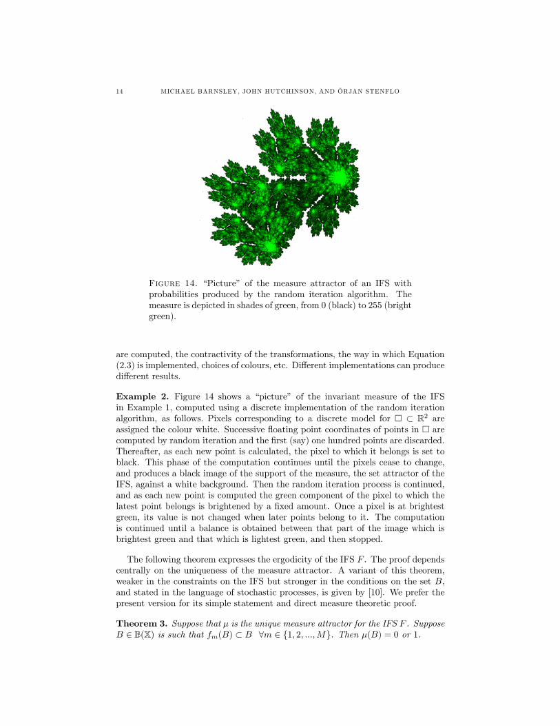
Figure 14. “Picture” of the measure attractor of an IFS withprobabilities produced by the random iteration algorithm. Themeasure is depicted in shades of green, from 0 (black) to 255 (brightgreen).
are computed, the contractivity of the transformations, the way in which Equation(2.3) is implemented, choices of colours, etc. Different implementations can producedifferent results.
Example 2. Figure 14 shows a “picture” of the invariant measure of the IFSin Example 1, computed using a discrete implementation of the random iterationalgorithm, as follows. Pixels corresponding to a discrete model for ¤ ⊂ R2 areassigned the colour white. Successive floating point coordinates of points in ¤ arecomputed by random iteration and the first (say) one hundred points are discarded.Thereafter, as each new point is calculated, the pixel to which it belongs is set toblack. This phase of the computation continues until the pixels cease to change,and produces a black image of the support of the measure, the set attractor of theIFS, against a white background. Then the random iteration process is continued,and as each new point is computed the green component of the pixel to which thelatest point belongs is brightened by a fixed amount. Once a pixel is at brightestgreen, its value is not changed when later points belong to it. The computationis continued until a balance is obtained between that part of the image which isbrightest green and that which is lightest green, and then stopped.
The following theorem expresses the ergodicity of the IFS F . The proof dependscentrally on the uniqueness of the measure attractor. A variant of this theorem,weaker in the constraints on the IFS but stronger in the conditions on the set B,and stated in the language of stochastic processes, is given by [10]. We prefer thepresent version for its simple statement and direct measure theoretic proof.
Theorem 3. Suppose that µ is the unique measure attractor for the IFS F . SupposeB ∈ B(X) is such that fm(B) ⊂ B ∀m ∈ 1, 2, ...,M. Then µ(B) = 0 or 1.
RANDOM IFSS 15
Proof. Let us define the measure µbB (µ restricted by B) by (µbB)(E) = µ(B∩E).The main point of the proof is to show that µbB is invariant under the IFS F . ( Asimilar result applies to µbBC where BC denotes the complement of B.)If E ⊂ BC , for any m, since fm(B) ⊂ B,
fm(µbB)(E) = µ(B ∩ f−1m (E)) = µ(∅) = 0.Moreover,
(2.4) µ(B) = fm(µbB)(X) = fm(µbB)(B).It follows that
µ(B) =MXm=1
pmfmµ(B) =MXm=1
pmfm(µbB)(B) +MXm=1
pmfm(µbBC)(B)
= µ(B) +MXm=1
pmfm(µbBC)(B) (from (2.4)).
Hence
(2.5)MXm=1
pmfm(µbBC)(B) = 0.
Hence for any measurable set E ⊂ X
(µbB)(E) = µ(B ∩E) =MXm=1
pmfmµ(B ∩E)
=MXm=1
pmfm(µbB)(B ∩E) +MXm=1
pmfm(µbBC)(B ∩E)
=MXm=1
pmfm(µbB)(E) + 0 (using (2.5)).
Thus µbB is invariant and so is either the zero measure or for some constant c ≥ 1we have cµbB = µ (by uniqueness)= µbB + µbBC . This implies µbBC = 0 and inparticular µ(BC) = 0 and µ(B) = 1. ¤
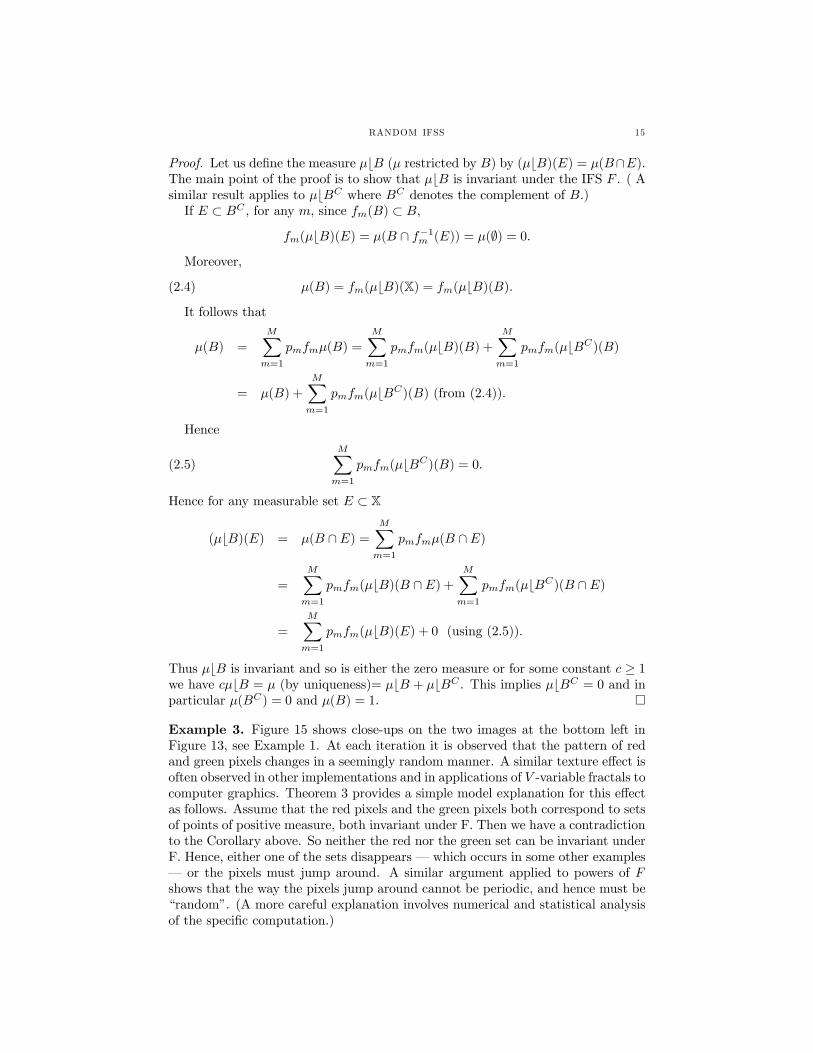
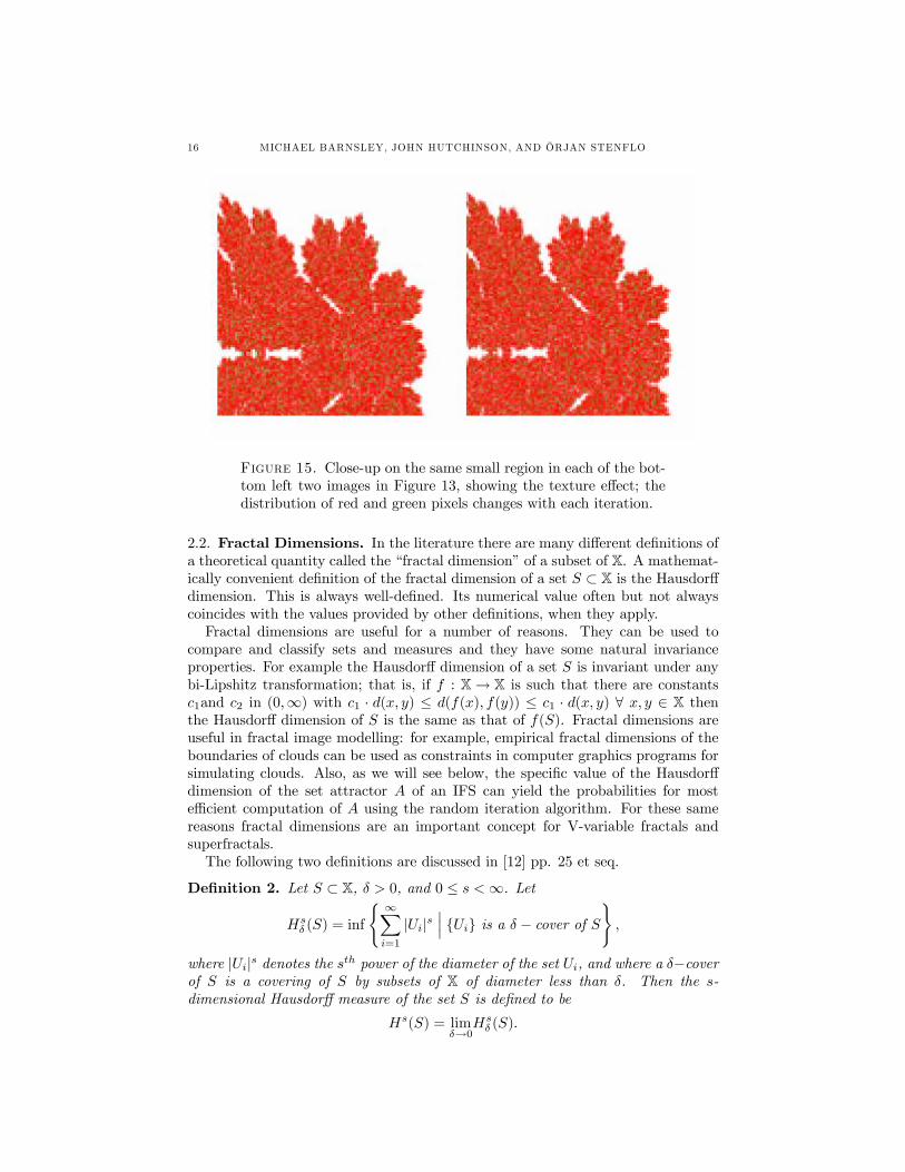
Example 3. Figure 15 shows close-ups on the two images at the bottom left inFigure 13, see Example 1. At each iteration it is observed that the pattern of redand green pixels changes in a seemingly random manner. A similar texture effect isoften observed in other implementations and in applications of V -variable fractals tocomputer graphics. Theorem 3 provides a simple model explanation for this effectas follows. Assume that the red pixels and the green pixels both correspond to setsof points of positive measure, both invariant under F. Then we have a contradictionto the Corollary above. So neither the red nor the green set can be invariant underF. Hence, either one of the sets disappears – which occurs in some other examples– or the pixels must jump around. A similar argument applied to powers of Fshows that the way the pixels jump around cannot be periodic, and hence must be“random”. (A more careful explanation involves numerical and statistical analysisof the specific computation.)
16 MICHAEL BARNSLEY, JOHN HUTCHINSON, AND ÖRJAN STENFLO
Figure 15. Close-up on the same small region in each of the bot-tom left two images in Figure 13, showing the texture effect; thedistribution of red and green pixels changes with each iteration.
2.2. Fractal Dimensions. In the literature there are many different definitions ofa theoretical quantity called the “fractal dimension” of a subset of X. A mathemat-ically convenient definition of the fractal dimension of a set S ⊂ X is the Hausdorffdimension. This is always well-defined. Its numerical value often but not alwayscoincides with the values provided by other definitions, when they apply.Fractal dimensions are useful for a number of reasons. They can be used to
compare and classify sets and measures and they have some natural invarianceproperties. For example the Hausdorff dimension of a set S is invariant under anybi-Lipshitz transformation; that is, if f : X→ X is such that there are constantsc1and c2 in (0,∞) with c1 · d(x, y) ≤ d(f(x), f(y)) ≤ c1 · d(x, y) ∀ x, y ∈ X thenthe Hausdorff dimension of S is the same as that of f(S). Fractal dimensions areuseful in fractal image modelling: for example, empirical fractal dimensions of theboundaries of clouds can be used as constraints in computer graphics programs forsimulating clouds. Also, as we will see below, the specific value of the Hausdorffdimension of the set attractor A of an IFS can yield the probabilities for mostefficient computation of A using the random iteration algorithm. For these samereasons fractal dimensions are an important concept for V-variable fractals andsuperfractals.The following two definitions are discussed in [12] pp. 25 et seq.
Definition 2. Let S ⊂ X, δ > 0, and 0 ≤ s <∞. Let
Hsδ (S) = inf
( ∞Xi=1
|Ui|s¯Ui is a δ − cover of S
),
where |Ui|s denotes the sth power of the diameter of the set Ui, and where a δ−coverof S is a covering of S by subsets of X of diameter less than δ. Then the s-dimensional Hausdorff measure of the set S is defined to be
Hs(S) = limδ→0
Hsδ (S).
RANDOM IFSS 17
The s-dimensional Hausdorff measure is a Borel measure but is not normallyeven σ-finite.
Definition 3. The Hausdorff dimension of the set S ⊂ X is defined to bedimH S = infs | Hs(S) = 0.
The following quantity is often called the fractal dimension of the set S. It canbe approximated in practical applications, by estimating the slope of the graph ofthe logarithm of the number of “boxes” of side length δ that intersect S, versus thelogarithm of δ.
Definition 4. The box-counting dimension of the set S ⊂ X is defined to be
dimB S = limδ→0
logNδ(S)
log(1/δ)
if and only if this limit exists, where Nδ(S) is the smallest number of sets of diameterδ > 0 that can cover S.
In order to provide a precise calculation of box-counting and Hausdorff dimensionof the attractor of an IFS we need the following condition.
Definition 5. The IFS F is said to obey the open set condition if there exists anon-empty open set O such that
F (O) =M[m=1
fm(O) ⊂ O,
andfm(O) ∩ fl(O) = ∅ if m 6= l.
The following theorem provides the Hausdorff dimension of the attractor of anIFS in some special cases.
Theorem 4. Let the IFS F consist of similitudes, that is fm(x) = smOmx + tmwhere Om is an orthonormal transformation on RK , sm ∈ (0, 1), and tm ∈ RK .Also let F obey the open set condition, and let A denote the set attractor of F .Then
dimH A = dimB A = D
where D is the unique solution of
(2.6)MXm=1
sDm = 1.
Moreover,0 < HD(A) <∞.
Proof. This theorem, in essence, was first proved by Moran in 1946, [22]. A fullproof is given in [12] p.118. ¤
A good choice for the probabilities, which ensures that the points obtained fromthe random iteration algorithm are distributed uniformly around the set attractorin case the open set condition applies, is pm = sDm. Note that the choice of Din Equation 2.6 is the unique value which makes (p1, p2, ..., pM ) into a probabilityvector.
18 MICHAEL BARNSLEY, JOHN HUTCHINSON, AND ÖRJAN STENFLO
2.3. Code Space. A good way of looking at an IFS F as in (2.1) is in terms ofthe associated code space Σ = 1, 2, ...,M∞. Members of Σ are infinite sequencesfrom the alphabet 1, 2, ...,M and indexed by N. We equip Σ with the metric dΣdefined for ω 6= κ by
dΣ(ω,κ) =1
Mk,
where k is the index of the first symbol at which ω and κ differ. Then (Σ, dΣ) is acompact metric space.
Theorem 5. Let A denote the set attractor of the IFS F . Then there exists acontinuous onto mapping F : Σ→ A, defined for all σ1σ2σ3... ∈ Σ by
F (σ1σ2σ3...) = limk→∞
fσ1 fσ2 ... fσk(x).
The limit is independent of x ∈ X and the convergence is uniform in x.
Proof. This result is contained in [16] Theorem 3.1(3). ¤
Definition 6. The point σ1σ2σ3... ∈ Σ is called an address of the point F (σ1σ2σ3...) ∈A.
Note that F : Σ→ A is not in general one-to-one.The following theorem characterizes the measure attractor of the IFS F as the
push-foward, under F : Σ → A, of an elementary measure ρ ∈ P(Σ), the measureattractor of a fundamental IFS on Σ.
Theorem 6. For each m ∈ 1, 2, ...,M define the shift operator sm : Σ→ Σ bysm(σ1σ2σ3...) = mσ1σ2σ3...
∀σ1σ2σ3... ∈ Σ. Then sm is a contraction mapping with contractivity factor 1M .
Consequently
S := Σ; s1,s2, ..., sM ; p1, p2, ..., pMis an IFS. Its set attractor is Σ. Its measure attractor is the unique measure π ∈P(Σ) such that
πω1ω2ω3... ∈ Σ|ω1 = σ1, ω2 = σ2, ..., ωk = σk = pσ1 · pσ2 · ... · pσk∀k ∈ N, ∀σ1, σ1, ..., σk ∈ 1, 2, ...,M.If µ is the measure attractor of the IFS F , with F : Σ→ A defined as in Theorem
5, then
µ = F (π).
Proof. This result is [16] Theorem 4.4(3) and (4). ¤
We call S the shift IFS on code space. It has been well studied in the contextof information theory and dynamical systems, see for example [7], and results canoften be lifted to the IFS F . For example, when the IFS is non-overlapping, theentropy (see [5] for the definition) of the stationary stochastic process associatedwith F is the same as that associated with the corresponding shift IFS, namely:−P pm log pm.
RANDOM IFSS 19
3. Trees of Iterated Function Systems and Random Fractals
3.1. SuperIFSs. Let (X, dX) be a compact metric space, and let M and N bepositive integers. For n ∈ 1, 2, ..., N let Fn denote the IFS
Fn = X; fn1 , fn2 , ...fnM ; pn1 , pn2 , ...pnMwhere each fnm : X → X is a Lipshitz function with Lipschitz constant 0 ≤ l < 1and the pnm ’s are probabilities with
MXm=1
pnm = 1, pnm ≥ 0 ∀ m,n.
Let
(3.1) F = X;F 1, F 2, ..., FN ;P1, P2, ..., PN,where the Pn’s are probabilities with
NXn=1
Pn = 1, Pn ≥ 0 ∀n ∈ 1, 2, ..., N.
Pn > 0 ∀n ∈ 1, 2, ..., N and PNn=1 Pn = 1.
As we will see in later sections, given any positive integer V we can use the setof IFSs F to construct a single IFS acting on H(X)V . In such cases we call F asuperIFS. Optionally, we will drop the specific reference to the probabilities.
3.2. Trees. We associate various collections of trees with F and the parametersM and N .Let T denote the (M -fold) set of finite sequences from 1, 2, ...,M, including
the empty sequence ∅. Then T is called a tree and the sequences are called thenodes of the tree. For i = i1i2...ik ∈ T let |i| = k. The number k is called the levelof the node σ. The bottom node ∅ is at level zero. If j = j1j2...jl ∈ T then ij isthe concatenated sequence i1i2...ikj1j2...jl.We define a level -k (M -fold) tree, or a tree of height k, Tk to be the set of nodes
of T of level less than or equal to k.A labelled tree is a function whose domain is a tree or a level-k tree. A limb
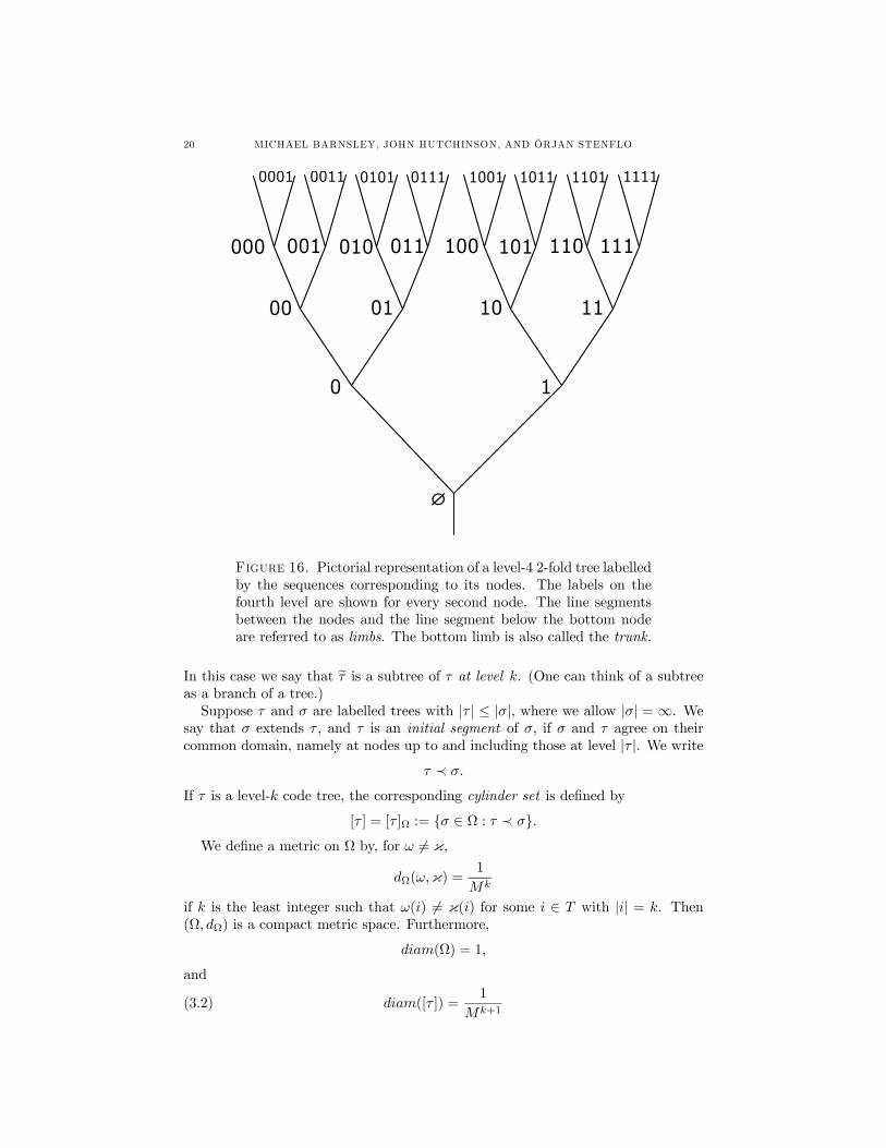
of a tree is either an ordered pair of nodes of the form (i, im) where i ∈ T andm ∈ 1, 2, ...,M, or the pair of nodes (∅, ∅), which is also called the trunk. Inrepresentations of labelled trees, as in Figures 16 and 19, limbs are represented byline segments and we attach the labels either to the nodes where line segments meetor to the line segments themselves, or possibly to both the nodes and limbs whena labelled tree is multivalued. For a two-valued labelled tree τ we will write
τ(i) = (τ(node i), τ(limb i)) for i ∈ T,
to denote the two components.A code tree is a labelled tree whose range is 1, 2, ..., N. We write
Ω = τ | τ : T → 1, 2, ..., Nfor the set of all infinite code trees.We define the subtree eτ : T → 1, 2, ..., N of a labelled tree τ : T → 1, 2, ..., N,
corresponding to a node i = i1i2...ik ∈ T, byeτ(j) = τ(ij) ∀ j ∈ T .
20 MICHAEL BARNSLEY, JOHN HUTCHINSON, AND ÖRJAN STENFLO
0 1
00 01 10 11
000 001 010 011 100 101 110 111
0001 0011 0101 0111 1001 1011 1101 1111
Figure 16. Pictorial representation of a level-4 2-fold tree labelledby the sequences corresponding to its nodes. The labels on thefourth level are shown for every second node. The line segmentsbetween the nodes and the line segment below the bottom nodeare referred to as limbs. The bottom limb is also called the trunk.
In this case we say that eτ is a subtree of τ at level k. (One can think of a subtreeas a branch of a tree.)Suppose τ and σ are labelled trees with |τ | ≤ |σ|, where we allow |σ| =∞. We
say that σ extends τ , and τ is an initial segment of σ, if σ and τ agree on theircommon domain, namely at nodes up to and including those at level |τ |. We write
τ ≺ σ.
If τ is a level-k code tree, the corresponding cylinder set is defined by
[τ ] = [τ ]Ω := σ ∈ Ω : τ ≺ σ.We define a metric on Ω by, for ω 6= κ,
dΩ(ω,κ) =1
Mk
if k is the least integer such that ω(i) 6= κ(i) for some i ∈ T with |i| = k. Then(Ω, dΩ) is a compact metric space. Furthermore,
diam(Ω) = 1,
and
(3.2) diam([τ ]) =1
Mk+1
RANDOM IFSS 21
whenever τ is a level-k code tree.The probabilities Pn associated with F in Equation (3.1) induce a natural prob-
ability distributionρ ∈ P(Ω)
on Ω. It is defined on cylinder sets [τ ] by
(3.3) ρ([τ ]) =Y
1≤|i|≤|τ |Pτ(i).
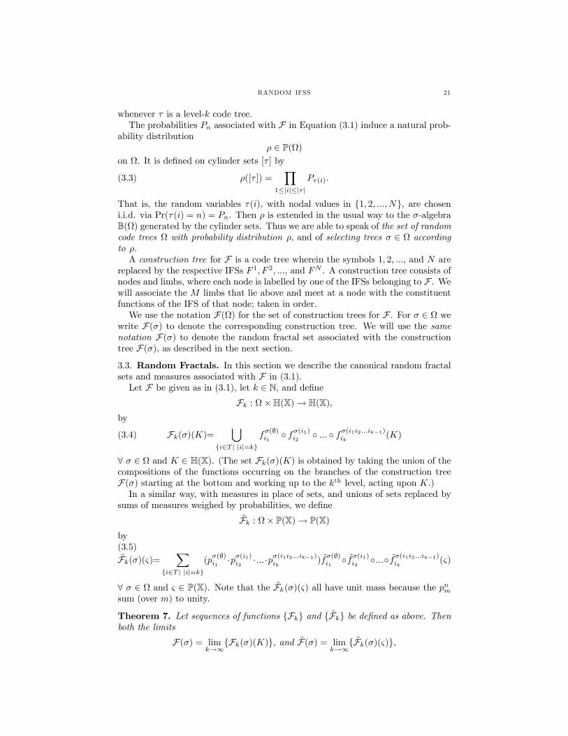
That is, the random variables τ(i), with nodal values in 1, 2, ...,N, are choseni.i.d. via Pr(τ(i) = n) = Pn. Then ρ is extended in the usual way to the σ-algebraB(Ω) generated by the cylinder sets. Thus we are able to speak of the set of randomcode trees Ω with probability distribution ρ, and of selecting trees σ ∈ Ω accordingto ρ.A construction tree for F is a code tree wherein the symbols 1, 2, ..., and N are
replaced by the respective IFSs F 1, F 2, ..., and FN . A construction tree consists ofnodes and limbs, where each node is labelled by one of the IFSs belonging to F . Wewill associate the M limbs that lie above and meet at a node with the constituentfunctions of the IFS of that node; taken in order.We use the notation F(Ω) for the set of construction trees for F . For σ ∈ Ω we
write F(σ) to denote the corresponding construction tree. We will use the samenotation F(σ) to denote the random fractal set associated with the constructiontree F(σ), as described in the next section.3.3. Random Fractals. In this section we describe the canonical random fractalsets and measures associated with F in (3.1).Let F be given as in (3.1), let k ∈ N, and define
Fk : Ω×H(X)→ H(X),by
(3.4) Fk(σ)(K)=[
i∈T | |i|=kfσ(∅)i1 fσ(i1)i2
... fσ(i1i2...ik−1)ik(K)
∀ σ ∈ Ω and K ∈ H(X). (The set Fk(σ)(K) is obtained by taking the union of thecompositions of the functions occurring on the branches of the construction treeF(σ) starting at the bottom and working up to the kth level, acting upon K.)In a similar way, with measures in place of sets, and unions of sets replaced by
sums of measures weighed by probabilities, we define
Fk : Ω× P(X)→ P(X)by(3.5)Fk(σ)(ς)=
Xi∈T | |i|=k
(pσ(∅)i1
·pσ(i1)i2·...·pσ(i1i2...ik−1)ik
)fσ(∅)i1 fσ(i1)i2
... fσ(i1i2...ik−1)ik(ς)
∀ σ ∈ Ω and ς ∈ P(X). Note that the Fk(σ)(ς) all have unit mass because the pnmsum (over m) to unity.
Theorem 7. Let sequences of functions Fk and Fk be defined as above. Thenboth the limits
F(σ) = limk→∞
Fk(σ)(K), and F(σ) = limk→∞
Fk(σ)(ς),
22 MICHAEL BARNSLEY, JOHN HUTCHINSON, AND ÖRJAN STENFLO
exist, are independent of K and ς, and the convergence (in the Hausdorff andMonge Kantorovitch metrics, respectively,) is uniform in σ, K, and ς. The resultingfunctions
F : Ω→ H(X) and F : Ω→ P(X)are continuous.
Proof. Make repeated use of the fact that, for fixed σ ∈ Ω, both mappings arecompositions of contraction mappings of contractivity l, by Theorem 1. ¤
Let
(3.6) H = F(σ) ∈ H(X)|σ ∈ Ω, and H = F(σ) ∈ P(X)|σ ∈ Ω.Similarly let
(3.7) P = F(ρ) = ρ F−1 ∈ P(H), and P = F(ρ) = ρ F−1 ∈ P(H).Definition 7. The sets H and H are called the sets of fractal sets and fractalmeasures, respectively, associated with F. These random fractal sets and measuresare said to be distributed according to P and P, respectively.
Random fractal sets and measures are hard to compute. There does not appearto be a general simple forwards (random iteration) algorithm for practical compu-tation of approximations to them in two-dimensions with affine maps, for example.The reason for this difficulty lies with the inconvenient manner in which the shiftoperator acts on trees σ ∈ Ω relative to the expressions (3.4) and (3.5).Definition 8. Both the set of IFSs Fn : n = 1, 2, .., N and the superIFS F aresaid to obey the (uniform) open set condition if there exists a non-empty open setO such that for each n ∈ 1, 2, .., N
Fn(O) =M[m=1
fnm(O) ⊂ O,
andfnm(O) ∩ fnl (O) = ∅ ∀ m, l ∈ 1, 2, ..,M with m 6= l.
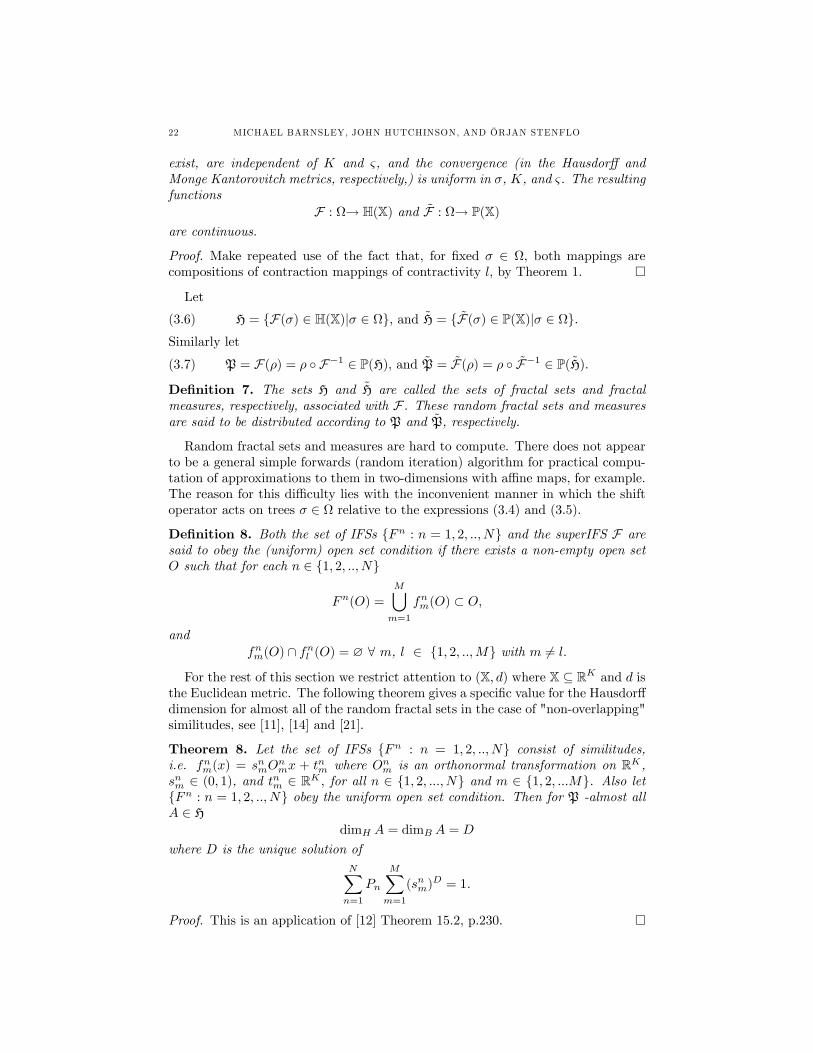
For the rest of this section we restrict attention to (X, d) where X ⊆ RK and d isthe Euclidean metric. The following theorem gives a specific value for the Hausdorffdimension for almost all of the random fractal sets in the case of "non-overlapping"similitudes, see [11], [14] and [21].
Theorem 8. Let the set of IFSs Fn : n = 1, 2, .., N consist of similitudes,i.e. fnm(x) = snmO
nmx + tnm where On
m is an orthonormal transformation on RK ,snm ∈ (0, 1), and tnm ∈ RK , for all n ∈ 1, 2, ..., N and m ∈ 1, 2, ...M. Also letFn : n = 1, 2, .., N obey the uniform open set condition. Then for P -almost allA ∈ H
dimH A = dimB A = D
where D is the unique solution ofNXn=1
Pn
MXm=1
(snm)D = 1.
Proof. This is an application of [12] Theorem 15.2, p.230. ¤
RANDOM IFSS 23
4. Contraction Mappings on Code Trees and the Space ΩV
4.1. Construction and Properties of ΩV . Let V ∈ N. This parameter willdescribe the variability of the trees and fractals that we are going to introduce. Let
ΩV = Ω×Ω× ...×Ω| z V TIMES
.
We refer to an element of ΩV as a grove. In this section we describe a certain IFSon ΩV , and discuss its set attractor ΩV : its points are (V -tuples of) code trees thatwe will call V -groves. We will find it convenient to label the trunk of each tree ina grove by its component index, from the set 1, 2, ..., V .One reason that we are interested in ΩV is that, as we shall see later, the set of
trees that occur in its components, called V -trees, provides the appropriate codespace for a V-variable superfractal.Next we describe mappings from ΩV to ΩV that comprise the IFS. The mappings
are denoted by ηa : ΩV → ΩV for a ∈ A where
(4.1) A := 1, 2, ..., N × 1, 2, ..., V MV .A typical index a ∈ A will be denoted
(4.2) a = (a1, a2, .., aV )
where
(4.3) av = (nv; vv,1, vv,2, ..., vv,M )
where nv ∈ 1, 2, ..., N and vv,m ∈ 1, 2, ..., V for m ∈ 1, 2, ...,M.Specifically, algebraically, the mapping ηa is defined in Equation (4.8) below. But
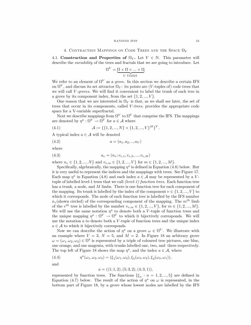
it is very useful to represent the indices and the mappings with trees. See Figure 17.Each map ηa in Equation (4.8) and each index a ∈ A may be represented by a V -tuple of labelled level-1 trees that we call (level-1) function trees. Each function treehas a trunk, a node, andM limbs. There is one function tree for each component ofthe mapping. Its trunk is labelled by the index of the component v ∈ 1, 2, ..., V towhich it corresponds. The node of each function tree is labelled by the IFS numbernv(shown circled) of the corresponding component of the mapping. The mth limbof the vth tree is labelled by the number vv,m ∈ 1, 2, ..., V , for m ∈ 1, 2, ...,M.We will use the same notation ηa to denote both a V -tuple of function trees andthe unique mapping ηa : ΩV → ΩV to which it bijectively corresponds. We willuse the notation a to denote both a V -tuple of function trees and the unique indexa ∈ A to which it bijectively corresponds.Now we can describe the action of ηa on a grove ω ∈ ΩV . We illustrate with
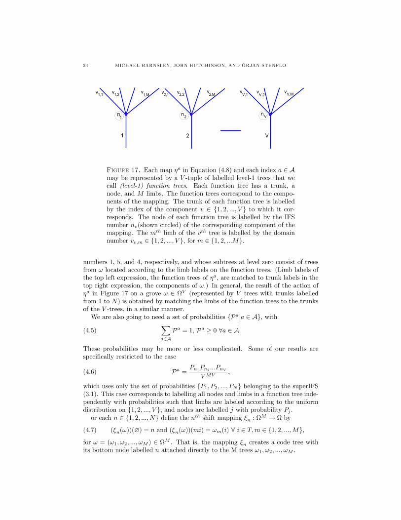
an example where V = 3, N = 5, and M = 2. In Figure 18 an arbitrary groveω = (ω1, ω2, ω3) ∈ Ω3 is represented by a triple of coloured tree pictures, one blue,one orange, and one magenta, with trunks labelled one, two, and three respectively.The top left of Figure 18 shows the map ηa, and the index a ∈ A, where(4.4) ηa(ω1, ω2, ω3) = (ξ1(ω1, ω2), ξ5(ω3, ω2), ξ4(ω3, ω1)),
anda = ((1; 1, 2), (5; 3, 2), (4; 3, 1)),
represented by function trees. The functions ξn : n = 1, 2, ..., 5 are defined inEquation (4.7) below. The result of the action of ηa on ω is represented, in thebottom part of Figure 18, by a grove whose lowest nodes are labelled by the IFS
24 MICHAEL BARNSLEY, JOHN HUTCHINSON, AND ÖRJAN STENFLO
v1,2 v1,Mv1,1
1
n1
v2,2 v2,Mv2,1
2
n2
vV,2
vV,MvV,1
V
nV
Figure 17. Each map ηa in Equation (4.8) and each index a ∈ Amay be represented by a V -tuple of labelled level-1 trees that wecall (level-1) function trees. Each function tree has a trunk, anode, and M limbs. The function trees correspond to the compo-nents of the mapping. The trunk of each function tree is labelledby the index of the component v ∈ 1, 2, ..., V to which it cor-responds. The node of each function tree is labelled by the IFSnumber nv(shown circled) of the corresponding component of themapping. The mth limb of the vth tree is labelled by the domainnumber vv,m ∈ 1, 2, ..., V , for m ∈ 1, 2, ...M.
numbers 1, 5, and 4, respectively, and whose subtrees at level zero consist of treesfrom ω located according to the limb labels on the function trees. (Limb labels ofthe top left expression, the function trees of ηa, are matched to trunk labels in thetop right expression, the components of ω.) In general, the result of the action ofηa in Figure 17 on a grove ω ∈ ΩV (represented by V trees with trunks labelledfrom 1 to N) is obtained by matching the limbs of the function trees to the trunksof the V -trees, in a similar manner.We are also going to need a set of probabilities Pa|a ∈ A, with
(4.5)Xa∈A
Pa = 1, Pa ≥ 0 ∀a ∈ A.
These probabilities may be more or less complicated. Some of our results arespecifically restricted to the case
(4.6) Pa =Pn1Pn2 ...PnV
VMV,
which uses only the set of probabilities P1, P2, ..., PN belonging to the superIFS(3.1). This case corresponds to labelling all nodes and limbs in a function tree inde-pendently with probabilities such that limbs are labeled according to the uniformdistribution on 1, 2, ..., V , and nodes are labelled j with probability Pj .or each n ∈ 1, 2, ..., N define the nth shift mapping ξn : ΩM → Ω by
(4.7) (ξn(ω))(∅) = n and (ξn(ω))(mi) = ωm(i) ∀ i ∈ T,m ∈ 1, 2, ...,M,for ω = (ω1, ω2, ..., ωM ) ∈ ΩM . That is, the mapping ξn creates a code tree withits bottom node labelled n attached directly to the M trees ω1, ω2, ..., ωM .
RANDOM IFSS 25
3,21 ,1
1
1 2
3
4
3 1
2
3 2
5
, ,
=
1
1
2
5
3
4
, ,
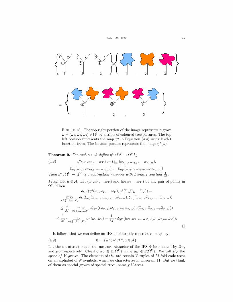
Figure 18. The top right portion of the image represents a groveω = (ω1, ω2, ω3) ∈ Ω3 by a triple of coloured tree pictures. The topleft portion represents the map ηa in Equation (4.4) using level-1function trees. The bottom portion represents the image ηa(ω).
Theorem 9. For each a ∈ A define ηa : ΩV → ΩV by(4.8) ηa(ω1, ω2, ..., ωV ) := (ξn1(ωv1,1 , ωv1,2 , ..., ωv1,M ),
ξn2(ωv2,1 , ωv2,2 , ..., ωv2,M ), ..., ξnV (ωvV,1 , ωvV,2 , ..., ωvV,M ))
Then ηa : ΩV → ΩV is a contraction mapping with Lipshitz constant 1M .
Proof. Let a ∈ A. Let (ω1, ω2, ..., ωV ) and (eω1,eω2,..., eωV ) be any pair of points inΩV . Then
dΩV (ηa(ω1, ω2, ..., ωV ), η
a(eω1,eω2,..., eωV )) =max
v∈1,2,...,V dΩ(ξnv(ωvv,1 , ωvv,2 , ..., ωvv,M ), ξnv(eωvv,1 , eωvv,2 , ..., eωvv,M ))
≤ 1
M· maxv∈1,2,...,V
dΩM ((ωvv,1 , ωvv,2 , ..., ωvv,M ), (eωvv,1,eωvv,2 ..., eωvv,M ))≤ 1
M· maxv∈1,2,...,V
dΩ(ωv, eωv) = 1
M· dΩV ((ω1, ω2, ..., ωV ), (eω1,eω2,..., eωV )).
¤
It follows that we can define an IFS Φ of strictly contractive maps by
(4.9) Φ = ΩV ; ηa,Pa, a ∈ A.Let the set attractor and the measure attractor of the IFS Φ be denoted by ΩV ,and µV respectively. Clearly, ΩV ∈ H(ΩV ) while µV ∈ P(ΩV ). We call ΩV thespace of V -groves. The elements of ΩV are certain V -tuples of M -fold code treeson an alphabet of N symbols, which we characterize in Theorem 11. But we thinkof them as special groves of special trees, namely V -trees.
26 MICHAEL BARNSLEY, JOHN HUTCHINSON, AND ÖRJAN STENFLO
For all v ∈ 1, 2, ..., V , let us define ΩV,v ⊂ ΩV to be the set of vth componentsof groves in ΩV . Also let ρV ∈ P(Ω) denote the marginal probability measuredefined by
(4.10) ρV (B) := µV (B,Ω,Ω, ...,Ω)∀B ∈ B(Ω).Theorem 10. For all v ∈ 1, 2, ..., V we have(4.11) ΩV,v = ΩV,1 := set of all V-trees.When the probabilities Pa|a ∈ A obey Equation (4.6), then starting at any initialgrove, the random distribution of trees ω ∈ Ω that occur in the vth componentsof groves produced by the random iteration algorithm corresponding to the IFS Φ,after n iteration steps, converge weakly to ρV independently of v, almost always, asn→∞.Proof. Let Ξ : Ω V → Ω V denote any map that permutes the coordinates. Then theIFS Φ = ΩV ; ηa,Pa, a ∈ A is invariant under Ξ, that is Φ = ΩV ;ΞηaΞ−1,Pa, a ∈A. It follows that ΞΩV = ΩV and ΞµV = µV . It follows that Equation (4.11)holds, and also that, in the obvious notation, for any (B1, B2, ..., BV ) ∈ (B(Ω))Vwe have
(4.12) µV (B1, B2, ..., BV ) = µV (Bσ1 , Bσ2 , ..., BσV ).
In particular
ρV (B) = µV (B,Ω,Ω, ...,Ω) = µV (Ω,Ω, ...,Ω, B,Ω, ...,Ω) ∀B ∈ B(Ω),where the “B” on the right-hand-side is in the vth position. Theorem 9 tells us thatwe can apply the random iteration algorithm (Theorem 2) to the IFS Φ. This yieldssequences of measures, denoted by µ(l)V : l = 1, 2, 3..., that converge weakly to µValmost always. In particular µ(l)V (B,Ω,Ω, ...,Ω) converges to ρV almost always. ¤Let L denote a set of fixed length vectors of labelled trees. We will say that
L and its elements have the property of V -variability, or that L and its elementsare V -variable, if and only if, for all ω ∈ L, the number of distinct subtrees of allcomponents of ω at level k is at most V , for each level k of the trees.
Theorem 11. Let ω ∈ ΩV . Then ω ∈ ΩV if and only ω contains at most V distinctsubtrees at any level (i.e. ω is V-variable). Also, if σ ∈ Ω, then σ is a V-tree if andonly if it is V-variable.
Proof. Let
S = ω ∈ ΩV | |subtrees of components of ω at level k| ≤ V, ∀ k ∈ N.Then S is closed: Let sn ∈ S converge to s∗. Suppose that s∗ /∈ S. Then, at somelevel k ∈ N, s∗ has more than V subtrees. There exists l ∈ N so that each distinctpair of these subtrees of s∗ first disagrees at some level less than l. Now choose nso large that sn agrees with s∗ through level (k + l) (i.e. dΩV (sn, s∗) < 1
M(k+l) ).Then sn has more than V distinct subtrees at level k, a contradiction. So s∗ ∈ S.Also S is non-empty: Let σ ∈ Ω be defined by σ(i) = 1 for all i ∈ T . Then
(σ, σ, ..., σ) ∈ S.Also S is invariant under the IFS Φ: Clearly any s ∈ S can be written s = ηa(es)
for some a ∈ A and es ∈ S. Also, if s ∈ S then ηa(s) ∈ S. So S = ∪ηa(S) | a ∈ A.Hence, by uniqueness, S must be the set attractor of Φ. That is, S = ΩV . This
proves the first claim in the Theorem.
RANDOM IFSS 27
It now follows that if σ ∈ Ω is a V -tree then it contains at most V distinctsubtrees at level k, for each k ∈ N. Conversely, it also follows that if σ ∈ Ω has thelatter property, then (σ, σ, ..., σ) ∈ ΩV , and so σ ∈ ΩV,1. ¤
Theorem 12. For all
dH(Ω)(ΩV,1,Ω) <1
V,
which implies thatlimV→∞
ΩV,1 = Ω,
where the convergence is in the Hausdorff metric. Let the probabilities Pa|a ∈ Aobey Equation (4.6). Then
(4.13) dP(Ω)(ρV , ρ) ≤ 1.4µM
V
¶ 14
which implieslimV→∞
ρV = ρ,
where ρ is the stationary measure on trees introduced in Section 3.2, and conver-gence is in the Monge Kantorovitch metric.
Proof. To prove the first part, let Mk+1 > V ≥ Mk. Let τ be any level-k codetree. Then τ is clearly V -variable and it can be extended to an infinite V -variablecode tree. It follows that [τ ] ∩ ΩV,1 6= ∅. The collection of such cylinder sets [τ ]forms a disjoint partition of Ω by subsets of diameter 1
Mk+1 , see Equation (3.2)),from which it follows that
dH(Ω)(ΩV,1,Ω) ≤ 1
Mk+1<1
V.
The first part of the theorem follows at once.For the proof of the second part, we refer to Section 4.4. ¤
Let ΣV = A∞. This is simply the code space corresponding to the IFS Φ definedin Equation (4.9). From Theorem 5 there exists a continuous onto mapping Φ :ΣV → ΩV defined by
Φ(a1a2a3...) = limk→∞
ηa1 ηa2 ... ηak(ω)for all a1a2a3... ∈ ΣV , for any ω. In the terminology of section 2.3 the sequencea1a2a3.. ∈ ΣV is an address of the V -grove Φ(a1a2a3...) ∈ ΩV and ΣV is the codespace for the set of V-groves ΩV . In general Φ : ΣV → ΩV is not one-to-one, as wewill see in Section 4.2.
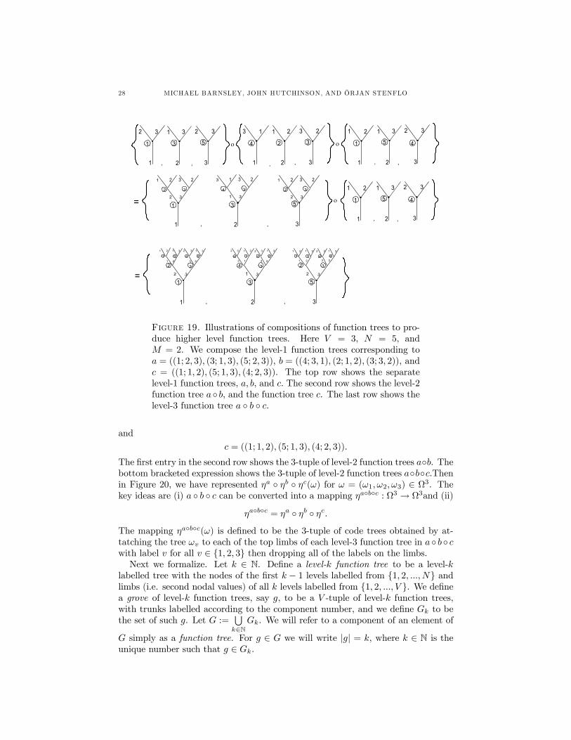
4.2. Compositions of the Mappings ηa. Compositions of the mappings ηa :ΩV → ΩV , a ∈ A, represented by V -tuples of level-1 function trees, as in Figure17, can be represented by higher level trees that we call level-k function trees.First we illustrate the ideas, then we formalize. In Figure 19 we illustate the
idea of composing V -tuples of function trees. In this example V = 3, N = 5, andM = 2. The top row shows the level-1 function trees corrresponding to a, b, c ∈ Agiven by
a = ((1; 2, 3), (3; 1, 3), (5; 2, 3)),
b = ((4; 3, 1), (2; 1, 2), (3; 3, 2)),
28 MICHAEL BARNSLEY, JOHN HUTCHINSON, AND ÖRJAN STENFLO
1
1
2 3
3
5
2 3
2
1 3
3
, , 1
4
3 1
3
3
3 2
2
1 2
2
, , 1
1
1 2
3
2 3
2
1 3
, ,
5 4
=
1
1
1 2
3
2 3
2
1 3
, ,
5 4
1
1
3
5
2
3
,
2
2
1
23
3
3 2 1
1
3
3
3
3 2 2
2
1
23
3
3 2
4
,
=
3
5
2
3
,
1 3
3
2
2
3
34
2 3 2 3
41 5
3
1 2 1 3
1 3 2
1 2 3 3
41 51
1 2 1 3
2 3 25
1
12
2
3
3
,
1 2 3 3
41 5
1
1 2 1 3
2 3 2
5
ο
οο
4
Figure 19. Illustrations of compositions of function trees to pro-duce higher level function trees. Here V = 3, N = 5, andM = 2. We compose the level-1 function trees corresponding toa = ((1; 2, 3), (3; 1, 3), (5; 2, 3)), b = ((4; 3, 1), (2; 1, 2), (3; 3, 2)), andc = ((1; 1, 2), (5; 1, 3), (4; 2, 3)). The top row shows the separatelevel-1 function trees, a, b, and c. The second row shows the level-2function tree a b, and the function tree c. The last row shows thelevel-3 function tree a b c.
and
c = ((1; 1, 2), (5; 1, 3), (4; 2, 3)).
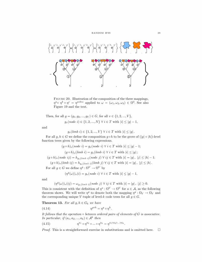
The first entry in the second row shows the 3-tuple of level-2 function trees ab. Thebottom bracketed expression shows the 3-tuple of level-2 function trees abc.Thenin Figure 20, we have represented ηa ηb ηc(ω) for ω = (ω1, ω2, ω3) ∈ Ω3. Thekey ideas are (i) a b c can be converted into a mapping ηabc : Ω3 → Ω3and (ii)
ηabc = ηa ηb ηc.The mapping ηabc(ω) is defined to be the 3-tuple of code trees obtained by at-tatching the tree ωv to each of the top limbs of each level-3 function tree in a b cwith label v for all v ∈ 1, 2, 3 then dropping all of the labels on the limbs.Next we formalize. Let k ∈ N. Define a level-k function tree to be a level-k
labelled tree with the nodes of the first k − 1 levels labelled from 1, 2, ..., N andlimbs (i.e. second nodal values) of all k levels labelled from 1, 2, ..., V . We definea grove of level-k function trees, say g, to be a V -tuple of level-k function trees,with trunks labelled according to the component number, and we define Gk to bethe set of such g. Let G :=
Sk∈N
Gk. We will refer to a component of an element of
G simply as a function tree. For g ∈ G we will write |g| = k, where k ∈ N is theunique number such that g ∈ Gk.
RANDOM IFSS 29
1
1
2 3
3
5
2 3
2
1 3
3
, , 1
4
3 1
3
3
3 2
2
1 2
2
, , 1
1
1 2
3
2 3
2
1 3
, ,
5 4
3,21 ,
3
5
2
3
,
3 2 34
41 5 41 55
1
1
2 3
,
41 55 4
=
oo
Figure 20. Illustration of the composition of the three mappings,ηa ηb ηc = ηabc applied to ω = (ω1, ω2, ω3) ∈ Ω3. See alsoFigure 19 and the text.
Then, for all g = (g1, g2, ..., gV ) ∈ G, for all v ∈ 1, 2, ..., V ,gv(node i) ∈ 1, 2, ..., N ∀ i ∈ T with |i| ≤ |g|− 1,
andgv(limb i) ∈ 1, 2, ..., V ∀ i ∈ T with |i| ≤ |g| .
For all g, h ∈ G we define the composition g h to be the grove of (|g|+ |h|)-levelfunction trees given by the following expressions.
(g h)v(node i) = gv(node i) ∀ i ∈ T with |i| ≤ |g|− 1;(g h)v(limb i) = gv(limb i) ∀ i ∈ T with |i| ≤ |g| ;
(g h)v(node ij) = hgv(limb i)(node j) ∀ ij ∈ T with |i| = |g| , |j| ≤ |h|− 1;(g h)v(limb ij) = hgv(limb i)(limb j) ∀ ij ∈ T with |i| = |g| , |j| ≤ |h| .
For all g ∈ G we define ηg : ΩV → ΩV by(ηg(ω))v(i) = gv(node i) ∀ i ∈ T with |i| ≤ |g|− 1,
and(ηg(ω))v(ij) = ωgv(limb i)(node j) ∀ ij ∈ T with |i| = |g| , |j| ≥ 0.
This is consistent with the definition of ηa : ΩV → ΩV for a ∈ A, as the followingtheorem shows. We will write ηg to denote both the mapping ηg : ΩV → ΩV andthe corresponding unique V -tuple of level-k code trees for all g ∈ G.
Theorem 13. For all g, h ∈ Gk we have
(4.14) ηgh = ηg ηh.It follows that the operation between ordered pairs of elements of G is associative.In particular, if (a1, a2, ..., ak) ∈ Ak then
(4.15) ηa1 ηa2 ... ηak = ηa1a2...ak .
Proof. This is a straightforward exercise in substitutions and is omitted here. ¤
30 MICHAEL BARNSLEY, JOHN HUTCHINSON, AND ÖRJAN STENFLO
We remark that Equations (4.15) and (4.14) allow us to work directly withfunction trees to construct, count, and track compositions of mappings ηa ∈ A.The space G also provides a convenient setting for contrasting the forwards andbackwards algorithms associated with the IFS Φ. For example, by composing func-tion trees in such as way as to build from the bottom up, which corresponds toa backwards algorithm, we find that we can construct a sequence of cylinder setapproximations to the first component ω1 of ω ∈ ΩV without having to computeapproximations to the other components.Let Gk(V ) ⊆ Gk denote the set of elements of Gk that can be written in the
form a1 a2 ... ak for some a = (a1, a2, ..., ak) ∈ Ak. (We remark that Gk(V ) isV -variable by a similar argument to the proof of Theorem 11.) Then we are able toestimate the measures of the cylinder sets [(ηa1a2...ak)1] by computing the prob-abilities of occurence of function trees g ∈ Gk(V ) such that (ηg)1 = (ηa1a2...ak)1built up starting from level-0 trees, with probabilities given by Equation (4.6), aswe do in the Section 4.4.The labeling of limbs in the approximating grove of function trees of level-k of
Φ(a1a2.....) defines the basic V -Variable dependence structure of Φ(a1a2.....). Wecall the code tree of limbs of a function tree the associated dependence tree.The grove of code trees for Φ(a1a2.....) is by definition totally determined by the
labels of the nodes. Nevertheless its grove of dependence trees contains all informa-tion concerning its V-Variable structure. The dependence tree is the characterizingskeleton of V -Variable fractals.
4.3. A direct characterization of the measure ρV . LetFn∞n=0 = Fn1 , ..., F
nV ∞n=0
be a sequence of random groves of level-1 function trees. Each random functiontree can be expressed as Fn
v = (Nnv , L
nv (1), ..., L
nv (M)) where the Nn
v ’s and Lnv ’scorresponds to random labellings of nodes and limbs respectively.We assume that the function trees Fn
v , are independent with Pr(Nnv = j) = Pj
and Pr(Lnv (m) = k) = 1/V for any v, k ∈ 1, .., V , n ∈ N, j ∈ 1, ..., N, andm ∈ 1, ...,M.First the family Ln1 , ..., LnV generates a random dependence tree, K : T →
1, .., V , in the following way. Let K(∅) = 1. If K(i1, ..., in) = j, for somej = 1, ..., V , then we define K(i1, ..., in, in+1) = Lnj (in+1).Given the dependence tree, let Ii = Nn
K(i) if |i| = n.The following theorem gives an alternative definition of ρV :
Theorem 14. ρV ([τ ]) = Pr(Ii = τ(i), ∀ |i| ≤ |τ |), where Iii∈T is defined asabove, and τ is a finite level code tree.
Proof. It is a straightforward exercise to check that (F0F1· · ·Fk−1)1 is a level-kfunction tree with nodes given by Ii|i|≤k−1, and limbs given by K(i)|i|≤k.Thus
Pr(Ii = τ(i), ∀ i with |i| ≤ k − 1)(4.16) = Pr((F0 F1 · · · Fk−1)1(node i) = τ(i), ∀ i with |i| ≤ k − 1).For
a = (a1, a2, ..., ak) ∈ Ak.
letPa = Pa1Pa2 ...Pak
RANDOM IFSS 31
denote the probability of selection of
ηa = ηa1 ηa2 ... ηak = ηa1a2...ak .
By the invariance of µV
µV =Xa∈Ak
Paηa(µV ).
Now let τ be a level-(k − 1) code tree. ThenρV ([τ ]) = µV (([τ ],Ω, ...,Ω)) =
Xa∈Ak
PaµV ((ηa)−1(([τ ],Ω, ...,Ω))
=X
a∈Ak|(ηa)1(node i)=τ(i), ∀ iPa.
From this and (4.16) it follows that ρV ([τ ]) = Pr(Ii = τ(i), ∀ i with |i| ≤k − 1). ¤
4.4. Proof of Theorem 12 Equation (4.13).
Proof. We say that a dependence tree is free up to level k, if at each level j, for1 ≤ j ≤ k, the M j limbs have distinct labels. If V is much bigger than M andk then it is clear that the probability of being free up to level k is close to unity.More precisely, if F is the event that dependence tree of (F0 F1 · · · Fk−1)1 isfree and V ≥Mk, then
ρV ([τ ]) = µV (([τ ],Ω, ...,Ω)) =Xa∈Ak
PaµV ((ηa)−1(([τ ],Ω, ...,Ω))
Pr(F ) =M−1Yi=1
µ1− i
V
¶M2−1Yi=1
µ1− i
V
¶...
Mk−1Yi=1
µ1− i
V
≥ 1− 1
V
M−1Xi=1
i+M2−1Xi=1
i+ ...+Mk−1Xi=1
i
≥ 1− 1
2V
¡M2 +M4 + ...+M2k
¢≥ 1− M2(k+1)
2V (M2 − 1) ≥ 1−2M2k
3V.
In the last steps we have assumed M ≥ 2.Let S be the event that (ηa1a2...ak)1 = τ . Then, using the independence of
the random variables labelling the nodes of a free function tree, and using Equation(3.3), we see that
Pr(S|F ) =Y
i∈T | 1≤|i|≤kPτ(i) = ρ([τ ]).
HenceρV ([τ ]) = Pr(S) = Pr(F ) Pr(S|F ) + Pr(FC) Pr(S|FC)
≤ Pr(S|F ) + Pr(FC) ≤ ρ ([τ ]) +2M2k
3V.
Similarly,ρV ([τ ]) ≥ Pr(F ) Pr(S|F )
32 MICHAEL BARNSLEY, JOHN HUTCHINSON, AND ÖRJAN STENFLO
≥ ρ ([τ ])− 2M2k
3V.
Hence
(4.17) |ρV ([τ ])− ρ([τ ])| 6 2M2k
3V.
In order to compute the Monge Kantorovitch distance dP(Ω)(ρV , ρ), suppose f :Ω→ R is Lipshitz with Lip f ≤ 1, i.e. |f(ω)−f( )| ≤ dΩ(ω, ) ∀ ω, ∈ Ω. Sincediam(Ω) = 1 we subtract a constant from f and so can assume |f | ≤ 1
2 withoutchanging the value of
Rfdρ− R fdρV .
For each level-k code tree τ ∈ Tk choose some ωτ ∈ [τ ] ⊆ Ω. It then follows that¯¯ZΩ
fdρ−ZΩ
fdρV
¯¯ =
¯¯Xτ∈Tk
Z[τ ]
fdρ−Z[τ ]
fdρV
¯¯ =
¯¯Xτ∈Tk
Z[τ ]
(f − f(ωτ ))dρ−Xτ∈Tk
Z[τ ]
((f − f(ωτ ))dρV +Xτ∈Tk
f(ωτ )(ρ([τ ])− ρV ([τ ]))
¯¯
≤ 1
Mk+1
Xτ∈Tk
ρ([τ ]) +1
Mk+1
Xτ∈Tk
ρV ([τ ]) +Xτ∈Tk
M2k
3V
= ϕ(k) :=2
Mk+1+
M3k
3V,
since diam [τ ] ≤ 1Mk+1 from Equation (3.2), |f(ωτ )| ≤ 1
2 , Lip f ≤ 1, ωτ ∈ [τ ] , andusing Equation 4.17. Choose x so that 2V
M = M4x. This is the value of x which
minimizes³
2Mx+1 +
M3x
3V
´. Choose k so that k ≤ x ≤ k + 1. Then
ϕ(k) ≤ 2µM
2V
¶ 14
+1
3V
µ2V
M
¶ 34
= 234
µM
V
¶ 14µ1 +
1
3M
≤ 7
214 3
µM
V
¶ 14
, (M ≥ 2).Hence Equation (4.13) is true. ¤
5. Superfractals
5.1. Contraction Mappings on HV and the Superfractal Set HV,1.
Definition 9. Let V ∈ N, let A be the index set introduced in Equation (4.1), letF be given as in Equation (3.1), and let probabilities Pa|a ∈ A be given as inEquation (4.5). Define
fa : HV → HV
by
(5.1) fa(K) = (M[m=1
fn1m (Kv1,m),M[m=1
fn2m (Kv2,m), ...M[m=1
fnVm (KvV,m))
∀K = (K1,K2, ...,KV ) ∈ HV ,∀a ∈ A. Let(5.2) FV := HV ; fa,Pa, a ∈ A.
RANDOM IFSS 33
Theorem 15. FV is an IFS with contractivity factor l.Proof. We only need to prove that the mapping fa : HV → HV is contractivewith contractivity factor l, ∀ a ∈ A. Note that, ∀K = (K1,K2, ...,KM ), L =(L1, L2, ..., LM ) ∈ HM ,
dH(M[m=1
fnm(Km),M[m=1
fnm(Lm))
≤ maxmdH(fnm(Km), f
nm(Lm))
≤ maxm
l · dH(Km, Lm)= l · dHM (K,L).
Hence, ∀(K1,K2, ...,KV ), (L1, L2, ..., LV ) ∈ HV ,
dHV (fa(K1,K2, ...,KV ), f
a(L1, L2, ..., LV ))
= maxvdH(
M[m=1
fnvm (Kvv,m),M[m=1
fnvm (Lvv,m))
≤ maxvl · d
HM((Kvv,1 ,Kvv,2 , ...,Kvv,M ),
(Lvv,1 , Lvv,2 , ..., Lvv,M ))≤ l · d
HV((K1,K2, ...,KV ), (L1, L2, ..., LV )).
¤
The theory of IFS in Section 2.1 applies to the IFS FV . It possesses a uniqueset attractor HV ∈ H(HV ), and a unique measure attractor PV ∈ P(HV ). The ran-dom iteration algorithm corresponding to the IFS FV may be used to approximatesequences of points (V - tuples of compact sets) in HV distributed according to theprobability measure PV .However, the individual components of these vectors in HV , certain special sub-
sets of X, are the objects we are interested in. Accordingly, for all v ∈ 1, 2, ..., V ,let us define HV,v ⊂ H to be the set of vth components of points in HV .Theorem 16. For all v ∈ 1, 2, ..., V we have
HV,v = HV,1.
When the probabilities in the superIFS FV are given by (4.6), then starting fromany initial V -tuple of non-empty compact subsets of X, the random distribution ofthe sets K ∈ H that occur in the vth component of vectors produced by the randomiteration algorithm after n initial steps converge weakly to the marginal probabilitymeasure
PV,1(B) := PV (B,H,H, ...,H)∀B ∈ B(H),independently of v, almost always, as n→∞.Proof. The direct way to prove this theorem is to parallel the proof of Theorem 10,using the maps fa : HV → HV | a ∈ A in place of the maps ηa : ΩV → ΩV |a ∈ A.However, an alternate proof follows with the aid of the map F : Ω→ H(X)
introduced in Theorem 7. We have put this alternate proof at the end of the proofof Theorem 17. ¤
34 MICHAEL BARNSLEY, JOHN HUTCHINSON, AND ÖRJAN STENFLO
Definition 10. We call HV,1 a superfractal set. Points in HV,1 are called V-variablefractal sets.
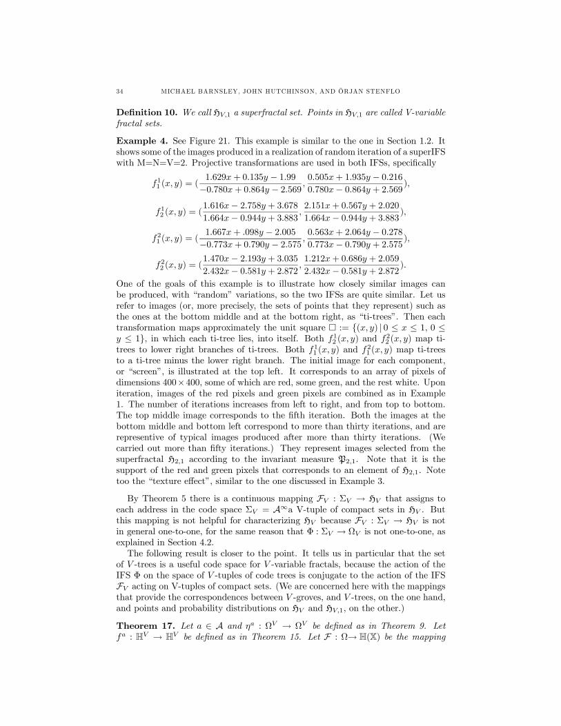
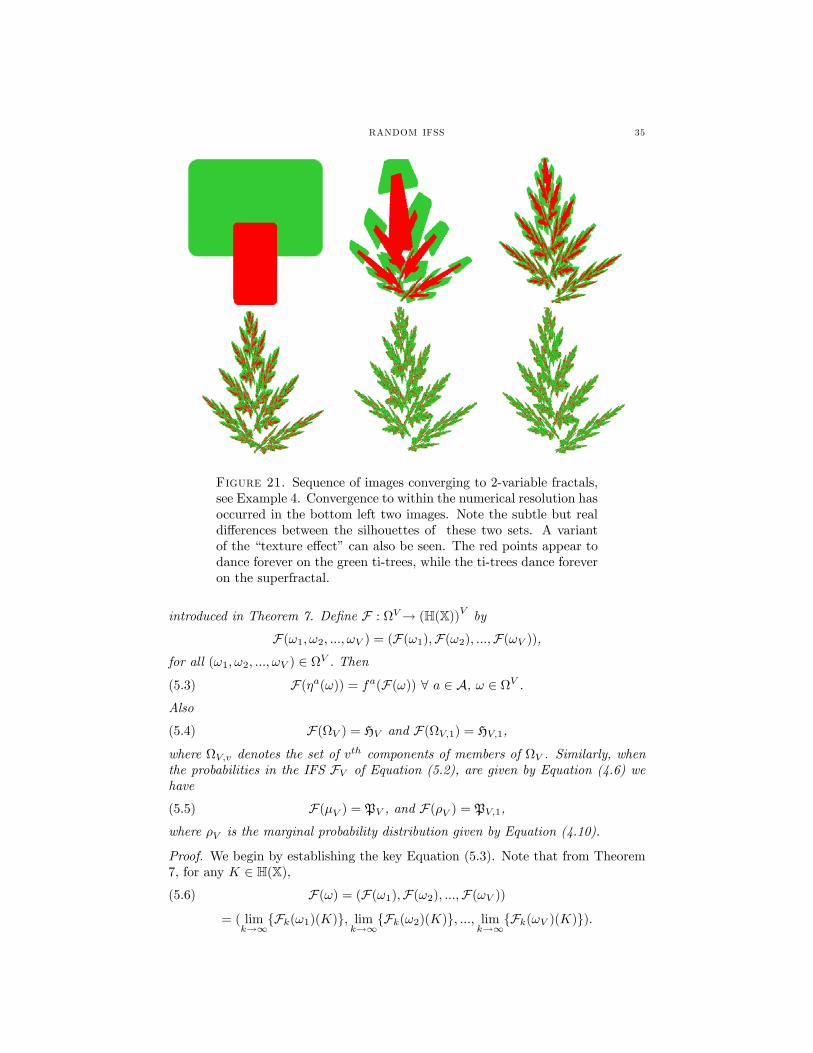
Example 4. See Figure 21. This example is similar to the one in Section 1.2. Itshows some of the images produced in a realization of random iteration of a superIFSwith M=N=V=2. Projective transformations are used in both IFSs, specifically
f11 (x, y) = (1.629x+ 0.135y − 1.99−0.780x+ 0.864y − 2.569 ,
0.505x+ 1.935y − 0.2160.780x− 0.864y + 2.569),
f12 (x, y) = (1.616x− 2.758y + 3.6781.664x− 0.944y + 3.883 ,
2.151x+ 0.567y + 2.020
1.664x− 0.944y + 3.883),
f21 (x, y) = (1.667x+ .098y − 2.005−0.773x+ 0.790y − 2.575 ,
0.563x+ 2.064y − 0.2780.773x− 0.790y + 2.575),
f22 (x, y) = (1.470x− 2.193y + 3.0352.432x− 0.581y + 2.872 ,
1.212x+ 0.686y + 2.059
2.432x− 0.581y + 2.872).One of the goals of this example is to illustrate how closely similar images canbe produced, with “random” variations, so the two IFSs are quite similar. Let usrefer to images (or, more precisely, the sets of points that they represent) such asthe ones at the bottom middle and at the bottom right, as “ti-trees”. Then eachtransformation maps approximately the unit square ¤ := (x, y) | 0 ≤ x ≤ 1, 0 ≤y ≤ 1, in which each ti-tree lies, into itself. Both f12 (x, y) and f22 (x, y) map ti-trees to lower right branches of ti-trees. Both f11 (x, y) and f21 (x, y) map ti-treesto a ti-tree minus the lower right branch. The initial image for each component,or “screen”, is illustrated at the top left. It corresponds to an array of pixels ofdimensions 400×400, some of which are red, some green, and the rest white. Uponiteration, images of the red pixels and green pixels are combined as in Example1. The number of iterations increases from left to right, and from top to bottom.The top middle image corresponds to the fifth iteration. Both the images at thebottom middle and bottom left correspond to more than thirty iterations, and arerepresentive of typical images produced after more than thirty iterations. (Wecarried out more than fifty iterations.) They represent images selected from thesuperfractal H2,1 according to the invariant measure P2,1. Note that it is thesupport of the red and green pixels that corresponds to an element of H2,1. Notetoo the “texture effect”, similar to the one discussed in Example 3.
By Theorem 5 there is a continuous mapping FV : ΣV → HV that assigns toeach address in the code space ΣV = A∞a V-tuple of compact sets in HV . Butthis mapping is not helpful for characterizing HV because FV : ΣV → HV is notin general one-to-one, for the same reason that Φ : ΣV → ΩV is not one-to-one, asexplained in Section 4.2.The following result is closer to the point. It tells us in particular that the set
of V -trees is a useful code space for V -variable fractals, because the action of theIFS Φ on the space of V -tuples of code trees is conjugate to the action of the IFSFV acting on V-tuples of compact sets. (We are concerned here with the mappingsthat provide the correspondences between V -groves, and V -trees, on the one hand,and points and probability distributions on HV and HV,1, on the other.)
Theorem 17. Let a ∈ A and ηa : ΩV → ΩV be defined as in Theorem 9. Letfa : HV → HV be defined as in Theorem 15. Let F : Ω→ H(X) be the mapping
RANDOM IFSS 35
Figure 21. Sequence of images converging to 2-variable fractals,see Example 4. Convergence to within the numerical resolution hasoccurred in the bottom left two images. Note the subtle but realdifferences between the silhouettes of these two sets. A variantof the “texture effect” can also be seen. The red points appear todance forever on the green ti-trees, while the ti-trees dance foreveron the superfractal.
introduced in Theorem 7. Define F : ΩV→ (H(X))V by
F(ω1, ω2, ..., ωV ) = (F(ω1),F(ω2), ...,F(ωV )),for all (ω1, ω2, ..., ωV ) ∈ ΩV . Then(5.3) F(ηa(ω)) = fa(F(ω)) ∀ a ∈ A, ω ∈ ΩV .Also
(5.4) F(ΩV ) = HV and F(ΩV,1) = HV,1,where ΩV,v denotes the set of vth components of members of ΩV . Similarly, whenthe probabilities in the IFS FV of Equation (5.2), are given by Equation (4.6) wehave
(5.5) F(µV ) = PV , and F(ρV ) = PV,1,
where ρV is the marginal probability distribution given by Equation (4.10).
Proof. We begin by establishing the key Equation (5.3). Note that from Theorem7, for any K ∈ H(X),(5.6) F(ω) = (F(ω1),F(ω2), ...,F(ωV ))
= ( limk→∞
Fk(ω1)(K), limk→∞
Fk(ω2)(K), ..., limk→∞
Fk(ωV )(K)).
36 MICHAEL BARNSLEY, JOHN HUTCHINSON, AND ÖRJAN STENFLO
The first component here exemplifies the others; and using Equation (3.4) it canbe written
(5.7) limk→∞
Fk(ω1)(K)
= limk→∞
[
i∈T | |i|=kfω1(∅)i1
fω1(i1)i2 ... fω1(i1i2...ik−1)ik
(K).
Since the convergence is uniform and all of the functions involved are continuous,we can interchange the lim with function operation at will. Look at
fa(F(ω)) = fa( limk→∞
Fk(ω1)(K), limk→∞
Fk(ω2)(K), ..., limk→∞
Fk(ωV )(K))= lim
k→∞fa(Fk(ω1)(K),Fk(ω2)(K), ...,Fk(ωV )(K)).
By the definition in Theorem 15, Equation 5.1, we have
fa(Fk(ω1)(K),Fk(ω2)(K), ...,Fk(ωV )(K))
= (M[m=1
fn1m (Fk(ωv1,m)(K)),M[m=1
fn2m (Fk(ωv2,m)(K)), ...,M[m=1
fnVm (Fk(ωvV,m)(K))).
By equation (3.4) the first component here isM[m=1
fn1m (Fk(ωv1,m)(K))
=M[m=1
fn1m ([
i∈T | |i|=kfωv1,m(∅)i1
fωv1,m(i1)i2 ... fωv1,m (i1i2...ik−1)ik
(K))
= Fk+1(ξn1(ωv1,1 , ωv1,2 , ..., ωv1,M ))(K),where we have used the definition in Equation (4.7). Hence
fa(F(ω)) = limk→∞
(fa(Fk(ω1)(K),Fk(ω2)(K), ...,Fk(ωV )(K)) =limk→∞
(Fk+1(ξn1(ωv1,1 , ωv1,2 , ..., ωv1,M ))(K),Fk+1(ξn2(ωv2,1 , ωv2,2 , ..., ωv2,M ))(K),...,Fk+1(ξnV (ωvV,1 , ωvV,2 , ..., ωvV,M ))(K)).
Comparing with Equations (5.6) and (5.7), we find that the right hand side hereconverges to F(ηa(ω)) as k →∞. So Equation (5.3) is true.Now consider the set F(ΩV ). We have
F(ΩV ) = F([a∈A
ηa(ΩV )) =[a∈A
F(ηa(ΩV )) =[a∈A
fa(F(ΩV )).
It follows by uniqueness that F(ΩV ) must be the set attractor of the IFS FV . HenceF(ΩV ) = HV which is the first statement in Equation (5.4). Now
F(ΩV,1) = F(ω1)|(ω1, ω2, ..., ωV ) ∈ ΩV = first component of (F(ω1),F(ω2), ...,F(ωV )) | (ω1, ω2, ..., ωV ) ∈ ΩV
= first component of F(ΩV ) = first component of HV = HV,1,which contains the second statement in Equation (5.4).In a similar manner we consider the push-forward under F : ΩV → HV of the
invariant measure µV of the IFS Φ = ΩV ; ηa,Pa, a ∈ A. F(µV ) is normalized,i.e. F(µV ) ∈ P(HV ), because F(µV )(HV ) = µV (F−1(HV )) = µV (Ω
V ). We now
RANDOM IFSS 37
show that F(µV ) is the measure attractor the IFS FV . The measure attractor ofthe IFS Φ obeys
µV =Xa∈A
Paηa(µV ).
Applying F to both sides (i.e. constructing the push-fowards) we obtain
F(µV ) = F(Xa∈A
Paηa(µV )) =Xa∈A
PaF(ηa(µV )) =Xa∈A
Pafa(F(µV )),
where in the last step we have used the key Equation (5.3). So F(µV ) is the measureattractor of the IFS FV . Using uniqueness, we conclude F(µV ) = PV which is thefirst equation in Equation (5.5). Finally, observe that, for all B ∈ B(H),
PV,1(B) = F(µV )(B,H,H, ...,H) = µV (F−1(B,H,H, ...,H))= µV ((F−1(B),F−1(H),F−1(H), ...,F−1(H))) (using Equation (5.6))
= µV ((F−1(B),Ω,Ω, ...,Ω)) (since F : Ω→ H)= ρV (F−1(B)) (by definition (4.10)) = F(ρV )(B).
This contains the second equation in Equation (5.5).In a similar way, we obtain the alternate proof of Theorem 16. Simply lift
Theorem 10 to the domain of the IFS FV using F : ΩV → HV . ¤The code tree Φ(a1a2a3...) is called a tree address of the V-variable fractal
F(a1a2a3...).The mapping F : ΩV,1 → HV,1 together with Theorem 11 provides a character-
ization of V-variable fractals as follows. At any “magnification”, any V-variablefractal set is made of V “forms” or “shapes”:
Theorem 18. LetM ∈ HV,1 be any V -variable fractal set. Let > 0 be given. ThenM is a finite union of continuous transformations of at most V distinct compactsubsets of X, and the diameter of each of these transformed sets is at most .
Proof. Choose n so that ln < . Note that
HV =[a∈A
fa(HV ) =[
(a1,a2,...,an)∈Afa1 fa2 ... fan(HV ).
Hence, since (M,M, ...,M) ∈ HV it follows that there exists (K1,K2, ...,KV ) ∈ HVsuch that
M ∈ first component of[
(a1,a2,...,an)∈Afa1 fa2 ... fan(K1,K2, ...,KV ).
Each set in the union has diameter at most . ¤Example 5. This example is similar to Example 4, with M=N=V=2. The goalis to illustrate Theorem 18. Figure 22 shows, from left to right, from top to bot-tom, a sequence of six successive images, illustrating successive 2-variable fractals,corresponding to a superIFS of two IFSs. Each IFS consists of two projective trans-formations, each mapping the unit square ¤ into itself. The images were obtainedby running the random iteration algorithm, as described in Section 1.2. The initialimage on each screen was a blue convex region contained in a 400×400 array repre-senting ¤, and the images shown correspond to one of the discretized screens afterforty, forty-one, forty-two, forty-three, forty-four, and forty-five iterations. The keyfeatures of the transformations can be deduced from the images. (For example,
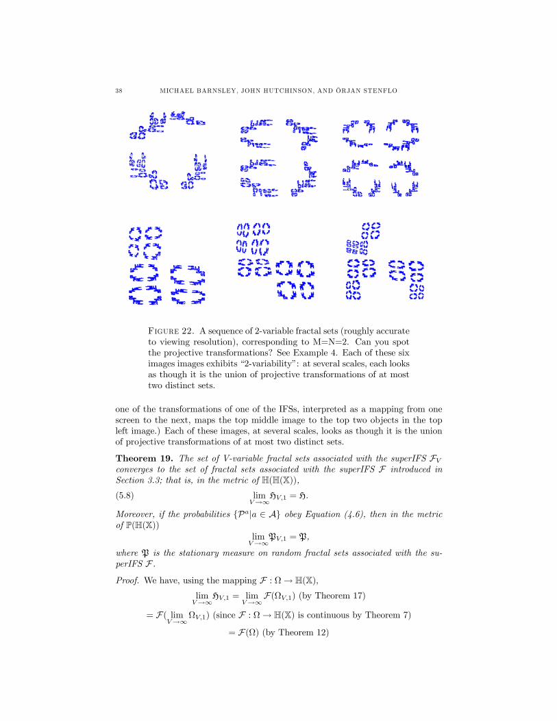
38 MICHAEL BARNSLEY, JOHN HUTCHINSON, AND ÖRJAN STENFLO
Figure 22. A sequence of 2-variable fractal sets (roughly accurateto viewing resolution), corresponding to M=N=2. Can you spotthe projective transformations? See Example 4. Each of these siximages images exhibits “2-variability”: at several scales, each looksas though it is the union of projective transformations of at mosttwo distinct sets.
one of the transformations of one of the IFSs, interpreted as a mapping from onescreen to the next, maps the top middle image to the top two objects in the topleft image.) Each of these images, at several scales, looks as though it is the unionof projective transformations of at most two distinct sets.
Theorem 19. The set of V-variable fractal sets associated with the superIFS FVconverges to the set of fractal sets associated with the superIFS F introduced inSection 3.3; that is, in the metric of H(H(X)),
(5.8) limV→∞
HV,1 = H.
Moreover, if the probabilities Pa|a ∈ A obey Equation (4.6), then in the metricof P(H(X))
limV→∞
PV,1 = P,
where P is the stationary measure on random fractal sets associated with the su-perIFS F .Proof. We have, using the mapping F : Ω→ H(X),
limV→∞
HV,1 = limV→∞
F(ΩV,1) (by Theorem 17)
= F( limV→∞
ΩV,1) (since F : Ω→ H(X) is continuous by Theorem 7)
= F(Ω) (by Theorem 12)
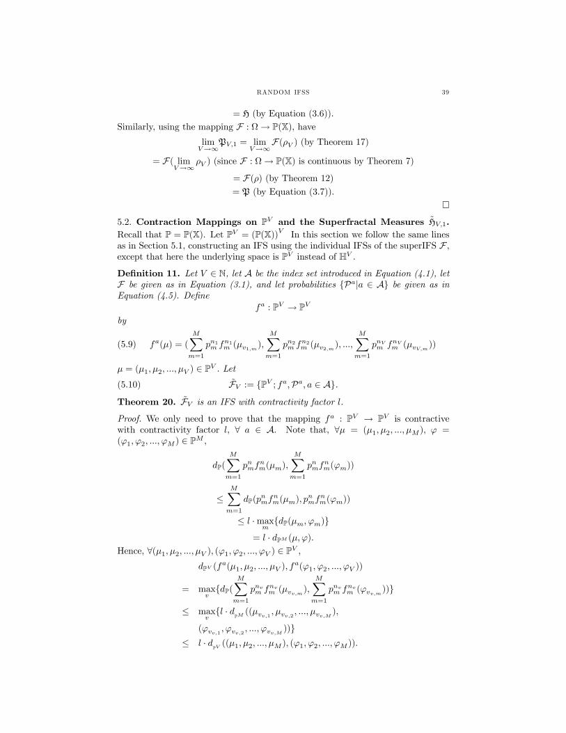
RANDOM IFSS 39
= H (by Equation (3.6)).Similarly, using the mapping F : Ω→ P(X), have
limV→∞
PV,1 = limV→∞
F(ρV ) (by Theorem 17)
= F( limV→∞
ρV ) (since F : Ω→ P(X) is continuous by Theorem 7)
= F(ρ) (by Theorem 12)
= P (by Equation (3.7)).¤
5.2. Contraction Mappings on PV and the Superfractal Measures HV,1.Recall that P = P(X). Let PV = (P(X))V In this section we follow the same linesas in Section 5.1, constructing an IFS using the individual IFSs of the superIFS F ,except that here the underlying space is PV instead of HV .
Definition 11. Let V ∈ N, let A be the index set introduced in Equation (4.1), letF be given as in Equation (3.1), and let probabilities Pa|a ∈ A be given as inEquation (4.5). Define
fa : PV → PV
by
(5.9) fa(µ) = (MXm=1
pn1m fn1m (µv1,m),MXm=1
pn2m fn2m (µv2,m), ...,MXm=1
pnVm fnVm (µvV,m))
µ = (µ1, µ2, ..., µV ) ∈ PV . Let(5.10) FV := PV ; fa,Pa, a ∈ A.Theorem 20. FV is an IFS with contractivity factor l.Proof. We only need to prove that the mapping fa : PV → PV is contractivewith contractivity factor l, ∀ a ∈ A. Note that, ∀µ = (µ1, µ2, ..., µM ), ϕ =(ϕ1, ϕ2, ..., ϕM ) ∈ PM ,
dP(MXm=1
pnmfnm(µm),
MXm=1
pnmfnm(ϕm))
≤MXm=1
dP(pnmf
nm(µm), p
nmf
nm(ϕm))
≤ l ·maxmdP(µm, ϕm)
= l · dPM (µ,ϕ).Hence, ∀(µ1, µ2, ..., µV ), (ϕ1, ϕ2, ..., ϕV ) ∈ PV ,
dPV (fa(µ1, µ2, ..., µV ), f
a(ϕ1, ϕ2, ..., ϕV ))
= maxvdP(
MXm=1
pnvm fnvm (µvv,m),MXm=1
pnvm fnvm (ϕvv,m))
≤ maxvl · d
PM((µvv,1 , µvv,2 , ..., µvv,M ),
(ϕvv,1 , ϕvv,2 , ..., ϕvv,M ))≤ l · d
PV((µ1, µ2, ..., µM ), (ϕ1, ϕ2, ..., ϕM )).
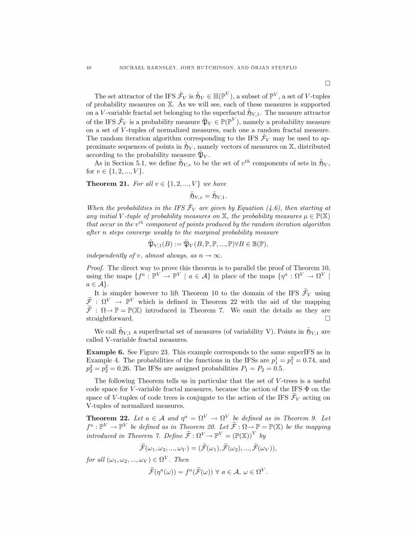
40 MICHAEL BARNSLEY, JOHN HUTCHINSON, AND ÖRJAN STENFLO
¤
The set attractor of the IFS FV is HV ∈ H(PV ), a subset of PV , a set of V -tuplesof probability measures on X. As we will see, each of these measures is supportedon a V -variable fractal set belonging to the superfactal HV,1. The measure attractorof the IFS FV is a probability measure PV ∈ P(PV ), namely a probability measureon a set of V -tuples of normalized measures, each one a random fractal measure.The random iteration algorithm corresponding to the IFS FV may be used to ap-proximate sequences of points in HV , namely vectors of measures on X, distributedaccording to the probability measure PV .As in Section 5.1, we define HV,v to be the set of vth components of sets in HV ,
for v ∈ 1, 2, ..., V .Theorem 21. For all v ∈ 1, 2, ..., V we have
HV,v = HV,1.
When the probabilities in the IFS FV are given by Equation (4.6), then starting atany initial V -tuple of probability measures on X, the probability measures µ ∈ P(X)that occur in the vth component of points produced by the random iteration algorithmafter n steps converge weakly to the marginal probability measure
PV,1(B) := PV (B,P,P, ...,P)∀B ∈ B(P),independently of v, almost always, as n→∞.Proof. The direct way to prove this theorem is to parallel the proof of Theorem 10,using the maps fa : PV → PV | a ∈ A in place of the maps ηa : ΩV → ΩV |a ∈ A.It is simpler however to lift Theorem 10 to the domain of the IFS eFV usingeF : ΩV → PV which is defined in Theorem 22 with the aid of the mappingeF : Ω→ P = P(X) introduced in Theorem 7. We omit the details as they are
straightforward. ¤
We call HV,1 a superfractal set of measures (of variability V). Points in HV,1 arecalled V-variable fractal measures.
Example 6. See Figure 23. This example corresponds to the same superIFS as inExample 4. The probabilities of the functions in the IFSs are p11 = p21 = 0.74, andp22 = p22 = 0.26. The IFSs are assigned probabilities P1 = P2 = 0.5.
The following Theorem tells us in particular that the set of V -trees is a usefulcode space for V -variable fractal measures, because the action of the IFS Φ on thespace of V -tuples of code trees is conjugate to the action of the IFS eFV acting onV-tuples of normalized measures.
Theorem 22. Let a ∈ A and ηa = ΩV → ΩV be defined as in Theorem 9. Letfa : PV → PV be defined as in Theorem 20. Let eF : Ω→ P = P(X) be the mappingintroduced in Theorem 7. Define eF : ΩV→ PV = (P(X))V byeF(ω1, ω2, ..., ωV ) = ( eF(ω1), eF(ω2), ..., eF(ωV )),for all (ω1, ω2, ..., ωV ) ∈ ΩV . TheneF(ηa(ω)) = fa( eF(ω)) ∀ a ∈ A, ω ∈ ΩV .

RANDOM IFSS 41
Figure 23. Three successive 2-variable fractal measures com-puted using the random iteration algorithm in Theorem 21 appliedto the superIFS in Example 6. The pixels in the support of eachmeasure are coloured either black or a shade of green, using a sim-ilar technique to the one used in Example 2. The intensity of thegreen of a pixel is a monotonic increasing function of the measureof the pixel.
Also eF(ΩV ) = eHV and eF(ΩV,1) = eHV,1,where ΩV,v denotes the set of vth components of members of ΩV . Similarly, whenthe probabilities in the IFS eFV of Equation (5.10), are given by Equation (4.6) wehave eF(µV ) = ePV , and eF(ρV ) = ePV,1,
where ρV is the marginal probability distribution given by Equation (4.10).
Proof. The proof is entirely parallel to the proof of Theorem 17, using eF in placeof F and is omitted. ¤
Definition 12. The code tree Φ(a1a2a3...) is called a tree address of the V-variablefractal measure FV (a1a2a3...).The mapping F : ΩV,1 → eHV,1 together with Theorem 11 allows us to charac-
terize V-variable fractals as follows:
Theorem 23. Let eµ ∈ eHV,1 be any V -variable fractal measure. Let > 0 begiven. Then eµ is a finite weighted superposition of continuous transformations ofat most V distinct normalized measures supported on compact subsets of X, and thediameter of the support of each of these transformed measures is at most .
Proof. Choose n so that ln < . Note thateHV = [a∈A
fa(eHV ) = [(a1,a2,...,an)∈A
fa1 fa2 ... fan(eHV ).Hence, since (eµ, eµ, ..., eµ) ∈ HV it follows that there exists ( 1, 2, ..., V ) ∈ HVsuch thateµ ∈ first component of
[(a1,a2,...,an)∈A
fa1 fa2 ... fan( 1, 2, ..., V ).
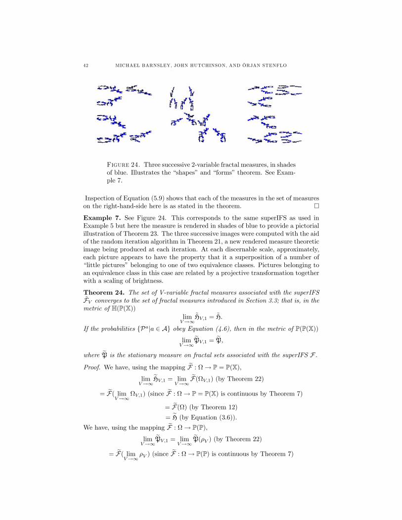
42 MICHAEL BARNSLEY, JOHN HUTCHINSON, AND ÖRJAN STENFLO
Figure 24. Three successive 2-variable fractal measures, in shadesof blue. Illustrates the “shapes” and “forms” theorem. See Exam-ple 7.
Inspection of Equation (5.9) shows that each of the measures in the set of measureson the right-hand-side here is as stated in the theorem. ¤Example 7. See Figure 24. This corresponds to the same superIFS as used inExample 5 but here the measure is rendered in shades of blue to provide a pictorialillustration of Theorem 23. The three successive images were computed with the aidof the random iteration algorithm in Theorem 21, a new rendered measure theoreticimage being produced at each iteration. At each discernable scale, approximately,each picture appears to have the property that it a superposition of a number of“little pictures” belonging to one of two equivalence classes. Pictures belonging toan equivalence class in this case are related by a projective transformation togetherwith a scaling of brightness.
Theorem 24. The set of V-variable fractal measures associated with the superIFSFV converges to the set of fractal measures introduced in Section 3.3; that is, in themetric of H(P(X))
limV→∞
HV,1 = H.
If the probabilities Pa|a ∈ A obey Equation (4.6), then in the metric of P(P(X))limV→∞
ePV,1 = eP,where eP is the stationary measure on fractal sets associated with the superIFS F .Proof. We have, using the mapping eF : Ω→ P = P(X),
limV→∞
eHV,1 = limV→∞
eF(ΩV,1) (by Theorem 22)
= eF( limV→∞
ΩV,1) (since eF : Ω→ P = P(X) is continuous by Theorem 7)
= eF(Ω) (by Theorem 12)
= eH (by Equation (3.6)).We have, using the mapping eF : Ω→ P(P),
limV→∞
ePV,1 = limV→∞
eP(ρV ) (by Theorem 22)
= eF( limV→∞
ρV ) (since eF : Ω→ P(P) is continuous by Theorem 7)
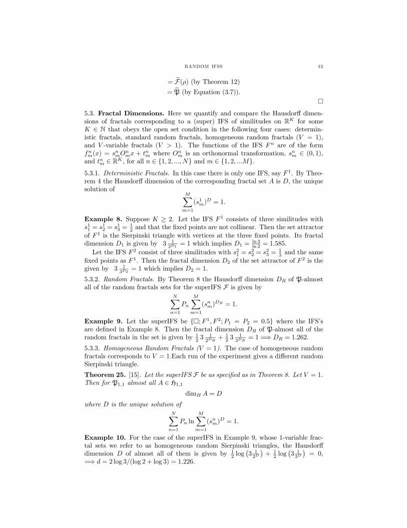
RANDOM IFSS 43
= eF(ρ) (by Theorem 12)
= eP (by Equation (3.7)).¤
5.3. Fractal Dimensions. Here we quantify and compare the Hausdorff dimen-sions of fractals corresponding to a (super) IFS of similitudes on RK for someK ∈ N that obeys the open set condition in the following four cases: determin-istic fractals, standard random fractals, homogeneous random fractals (V = 1),and V -variable fractals (V > 1). The functions of the IFS Fn are of the formfnm(x) = snmO
nmx + tnm where On
m is an orthonormal transformation, snm ∈ (0, 1),and tnm ∈ RK , for all n ∈ 1, 2, ...,N and m ∈ 1, 2, ...M.5.3.1. Deterministic Fractals. In this case there is only one IFS, say F 1. By Theo-rem 4 the Hausdorff dimension of the corresponding fractal set A is D, the uniquesolution of
MXm=1
(s1m)D = 1.
Example 8. Suppose K ≥ 2. Let the IFS F 1 consists of three similitudes withs11 = s12 = s13 =
12 and that the fixed points are not collinear. Then the set attractor
of F 1 is the Sierpinski triangle with vertices at the three fixed points. Its fractaldimension D1 is given by 3 1
2D1= 1 which implies D1 =
ln 3ln 2 = 1.585.
Let the IFS F 2 consist of three similitudes with s21 = s22 = s23 =13 and the same
fixed points as F 1. Then the fractal dimension D2 of the set attractor of F 2 is thegiven by 3 1
3D2= 1 which implies D2 = 1.
5.3.2. Random Fractals. By Theorem 8 the Hausdorff dimension DR of P-almostall of the random fractals sets for the superIFS F is given by
NXn=1
Pn
MXm=1
(snm)DR = 1.
Example 9. Let the superIFS be ¤;F 1, F 2;P1 = P2 = 0.5 where the IFS’sare defined in Example 8. Then the fractal dimension DR of P-almost all of therandom fractals in the set is given by 1
2 31
2DR+ 1
2 31
3DR= 1 =⇒ DR = 1.262.
5.3.3. Homogeneous Random Fractals (V = 1). The case of homogeneous randomfractals corresponds to V = 1.Each run of the experiment gives a different randomSierpinski triangle.
Theorem 25. [15]. Let the superIFS F be as specified as in Theorem 8. Let V = 1.Then for P1,1 almost all A ∈ H1,1
dimH A = D
where D is the unique solution ofNXn=1
Pn lnMXm=1
(snm)D = 1.
Example 10. For the case of the superIFS in Example 9, whose 1-variable frac-tal sets we refer to as homogeneous random Sierpinski triangles, the Hausdorffdimension D of almost all of them is given by 1
2 log¡3 12D
¢+ 1
2 log¡3 13D
¢= 0,
=⇒ d = 2 log 3/(log 2 + log 3) = 1.226.
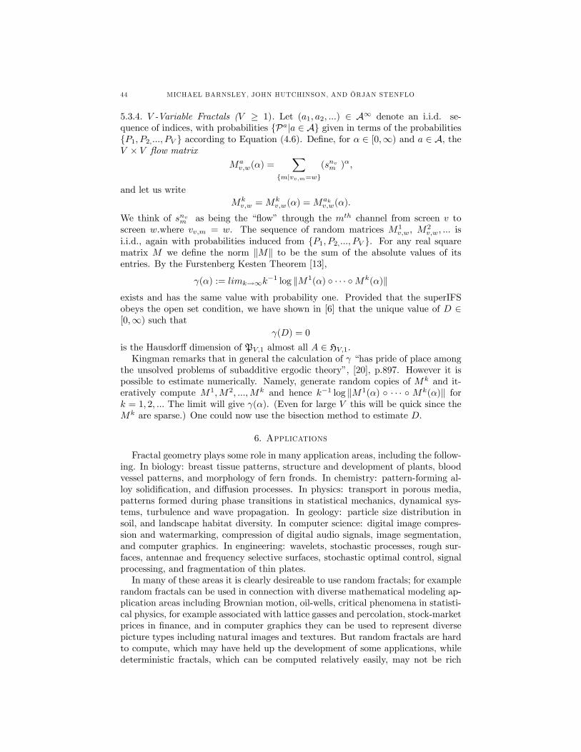
44 MICHAEL BARNSLEY, JOHN HUTCHINSON, AND ÖRJAN STENFLO
5.3.4. V -Variable Fractals (V ≥ 1). Let (a1, a2, ...) ∈ A∞ denote an i.i.d. se-quence of indices, with probabilities Pa|a ∈ A given in terms of the probabilitiesP1, P2,..., PV according to Equation (4.6). Define, for α ∈ [0,∞) and a ∈ A, theV × V flow matrix
Mav,w(α) =
Xm|vv,m=w
(snvm )α,
and let us writeMk
v,w =Mkv,w(α) =Mak
v,w(α).
We think of snvm as being the “flow” through the mth channel from screen v toscreen w.where vv,m = w. The sequence of random matrices M1
v,w, M2v,w, ... is
i.i.d., again with probabilities induced from P1, P2,..., PV . For any real squarematrix M we define the norm kMk to be the sum of the absolute values of itsentries. By the Furstenberg Kesten Theorem [13],
γ(α) := limk→∞k−1 log kM1(α) · · · Mk(α)kexists and has the same value with probability one. Provided that the superIFSobeys the open set condition, we have shown in [6] that the unique value of D ∈[0,∞) such that
γ(D) = 0
is the Hausdorff dimension of PV,1 almost all A ∈ HV,1.Kingman remarks that in general the calculation of γ “has pride of place among
the unsolved problems of subadditive ergodic theory”, [20], p.897. However it ispossible to estimate numerically. Namely, generate random copies of Mk and it-eratively compute M1,M2, ...,Mk and hence k−1 log kM1(α) · · · Mk(α)k fork = 1, 2, ... The limit will give γ(α). (Even for large V this will be quick since theMk are sparse.) One could now use the bisection method to estimate D.
6. Applications
Fractal geometry plays some role in many application areas, including the follow-ing. In biology: breast tissue patterns, structure and development of plants, bloodvessel patterns, and morphology of fern fronds. In chemistry: pattern-forming al-loy solidification, and diffusion processes. In physics: transport in porous media,patterns formed during phase transitions in statistical mechanics, dynamical sys-tems, turbulence and wave propagation. In geology: particle size distribution insoil, and landscape habitat diversity. In computer science: digital image compres-sion and watermarking, compression of digital audio signals, image segmentation,and computer graphics. In engineering: wavelets, stochastic processes, rough sur-faces, antennae and frequency selective surfaces, stochastic optimal control, signalprocessing, and fragmentation of thin plates.In many of these areas it is clearly desireable to use random fractals; for example
random fractals can be used in connection with diverse mathematical modeling ap-plication areas including Brownian motion, oil-wells, critical phenomena in statisti-cal physics, for example associated with lattice gasses and percolation, stock-marketprices in finance, and in computer graphics they can be used to represent diversepicture types including natural images and textures. But random fractals are hardto compute, which may have held up the development of some applications, whiledeterministic fractals, which can be computed relatively easily, may not be rich
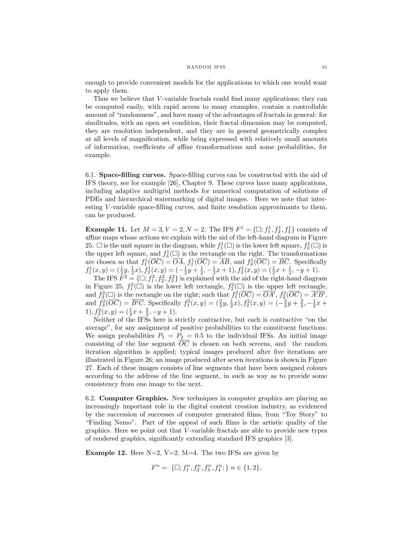
RANDOM IFSS 45
enough to provide convenient models for the applications to which one would wantto apply them.Thus we believe that V -variable fractals could find many applications; they can
be computed easily, with rapid access to many examples, contain a controllableamount of “randomness”, and have many of the advantages of fractals in general: forsimilitudes, with an open set condition, their fractal dimension may be computed,they are resolution independent, and they are in general geometrically complexat all levels of magnification, while being expressed with relatively small amountsof information, coefficients of affine transformations and some probabilities, forexample.
6.1. Space-filling curves. Space-filling curves can be constructed with the aid ofIFS theory, see for example [26], Chapter 9. These curves have many applications,including adaptive multigrid methods for numerical computation of solutions ofPDEs and hierarchical watermarking of digital images. Here we note that inter-esting V -variable space-filling curves, and finite resolution approximants to them,can be produced.
Example 11. Let M = 3, V = 2, N = 2. The IFS F 1 = ¤; f11 , f12 , f13 consists ofaffine maps whose actions we explain with the aid of the left-hand diagram in Figure25. ¤ is the unit square in the diagram, while f11 (¤) is the lower left square, f12 (¤) isthe upper left square, and f13 (¤) is the rectangle on the right. The transformationsare chosen so that f11 (OC) = OA, f12 (OC) = AB, and f13 (OC) = BC. Specificallyf11 (x, y) = (
12y,
12x), f
12 (x, y) = (−12y + 1
2 ,−12x+ 1), f13 (x, y) = ( 12x+ 12 ,−y + 1).
The IFS F 2 = ¤; f21 , f22 , f23 is explained with the aid of the right-hand diagramin Figure 25; f21 (¤) is the lower left rectangle, f22 (¤) is the upper left rectangle,and f23 (¤) is the rectangle on the right; such that f21 (OC) = OA0, f22 (OC) = A0B0,and f23 (OC) = B0C. Specifically f21 (x, y) = (
23y,
12x), f
22 (x, y) = (−23y + 2
3 ,−12x +1), f23 (x, y) = (
13x+
23 ,−y + 1).
Neither of the IFSs here is strictly contractive, but each is contractive “on theaverage”, for any assignment of positive probabilities to the constituent functions.We assign probabilities P1 = P2 = 0.5 to the individual IFSs. An initial imageconsisting of the line segment OC is chosen on both screens, and the randomiteration algorithm is applied; typical images produced after five iterations areillustrated in Figure 26; an image produced after seven iterations is shown in Figure27. Each of these images consists of line segments that have been assigned coloursaccording to the address of the line segment, in such as way as to provide someconsistency from one image to the next.
6.2. Computer Graphics. New techniques in computer graphics are playing anincreasingly important role in the digital content creation industry, as evidencedby the succession of successes of computer generated films, from “Toy Story” to“Finding Nemo”. Part of the appeal of such films is the artistic quality of thegraphics. Here we point out that V -variable fractals are able to provide new typesof rendered graphics, significantly extending standard IFS graphics [3].
Example 12. Here N=2, V=2, M=4. The two IFSs are given by
Fn = ¤; fn1 , fn2 , fn3 , fn4 ; n ∈ 1, 2,
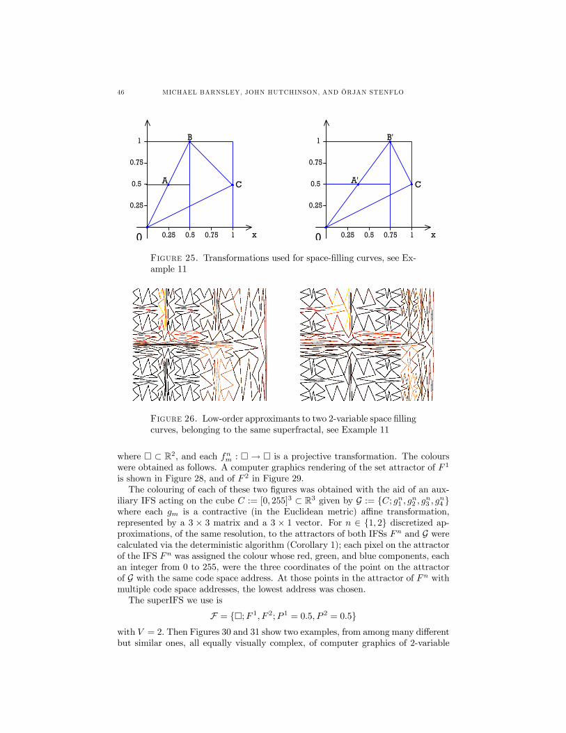
46 MICHAEL BARNSLEY, JOHN HUTCHINSON, AND ÖRJAN STENFLO
0.25 0.75 10.50
0.25
0.5
0.75
1
x 0.25 0.75 10.50
0.25
0.5
0.75
1 B'
CA'
x
A
B
C
Figure 25. Transformations used for space-filling curves, see Ex-ample 11
Figure 26. Low-order approximants to two 2-variable space fillingcurves, belonging to the same superfractal, see Example 11
where ¤ ⊂ R2, and each fnm : ¤ → ¤ is a projective transformation. The colourswere obtained as follows. A computer graphics rendering of the set attractor of F 1
is shown in Figure 28, and of F 2 in Figure 29.The colouring of each of these two figures was obtained with the aid of an aux-
iliary IFS acting on the cube C := [0, 255]3 ⊂ R3 given by G := C; gn1 , gn2 , gn3 , gn4 where each gm is a contractive (in the Euclidean metric) affine transformation,represented by a 3 × 3 matrix and a 3 × 1 vector. For n ∈ 1, 2 discretized ap-proximations, of the same resolution, to the attractors of both IFSs Fn and G werecalculated via the deterministic algorithm (Corollary 1); each pixel on the attractorof the IFS Fn was assigned the colour whose red, green, and blue components, eachan integer from 0 to 255, were the three coordinates of the point on the attractorof G with the same code space address. At those points in the attractor of Fn withmultiple code space addresses, the lowest address was chosen.The superIFS we use is
F = ¤;F 1, F 2;P 1 = 0.5, P 2 = 0.5with V = 2. Then Figures 30 and 31 show two examples, from among many differentbut similar ones, all equally visually complex, of computer graphics of 2-variable
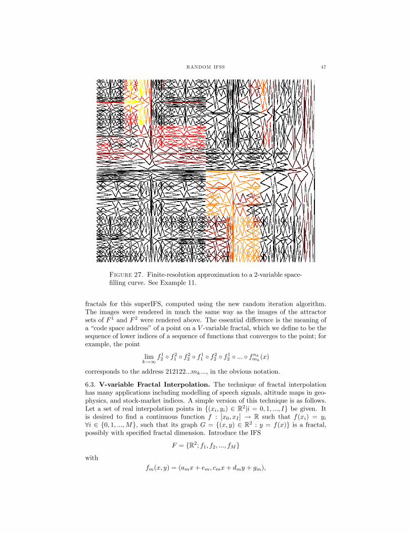
RANDOM IFSS 47
Figure 27. Finite-resolution approximation to a 2-variable space-filling curve. See Example 11.
fractals for this superIFS, computed using the new random iteration algorithm.The images were rendered in much the same way as the images of the attractorsets of F 1 and F 2 were rendered above. The essential difference is the meaning ofa “code space address” of a point on a V -variable fractal, which we define to be thesequence of lower indices of a sequence of functions that converges to the point; forexample, the point
limk→∞
f12 f21 f22 f11 f22 f12 ... fnkmk(x)
corresponds to the address 212122...mk..., in the obvious notation.
6.3. V-variable Fractal Interpolation. The technique of fractal interpolationhas many applications including modelling of speech signals, altitude maps in geo-physics, and stock-market indices. A simple version of this technique is as follows.Let a set of real interpolation points in (xi, yi) ∈ R2|i = 0, 1, ..., I be given. Itis desired to find a continuous function f : [x0, xI ] → R such that f(xi) = yi∀i ∈ 0, 1, ...,M, such that its graph G = (x, y) ∈ R2 : y = f(x) is a fractal,possibly with specified fractal dimension. Introduce the IFS
F = R2; f1, f2, ..., fMwith
fm(x, y) = (amx+ em, cmx+ dmy + gm),
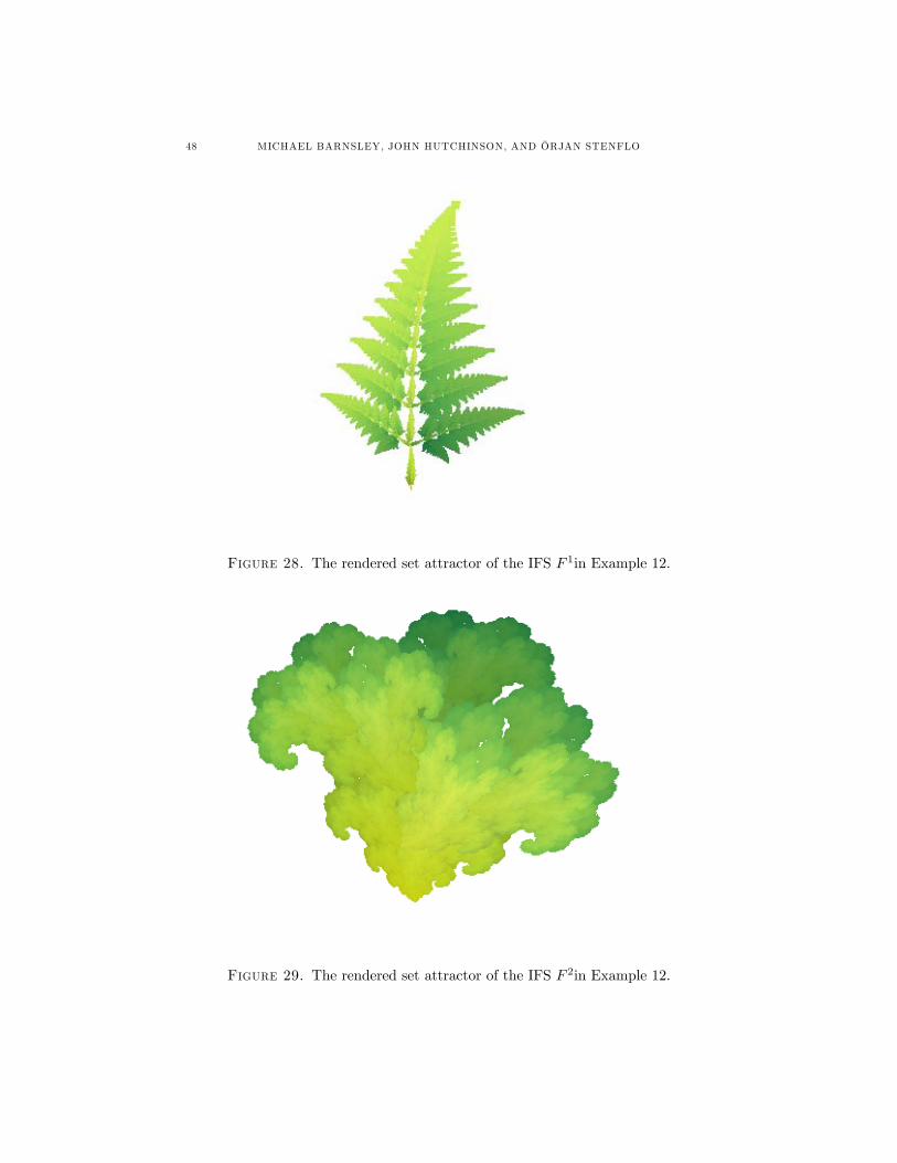
48 MICHAEL BARNSLEY, JOHN HUTCHINSON, AND ÖRJAN STENFLO
Figure 28. The rendered set attractor of the IFS F 1in Example 12.
Figure 29. The rendered set attractor of the IFS F 2in Example 12.
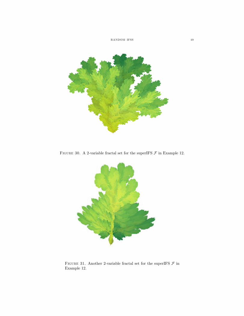
RANDOM IFSS 49
Figure 30. A 2-variable fractal set for the superIFS F in Example 12.
Figure 31. Another 2-variable fractal set for the superIFS F inExample 12.
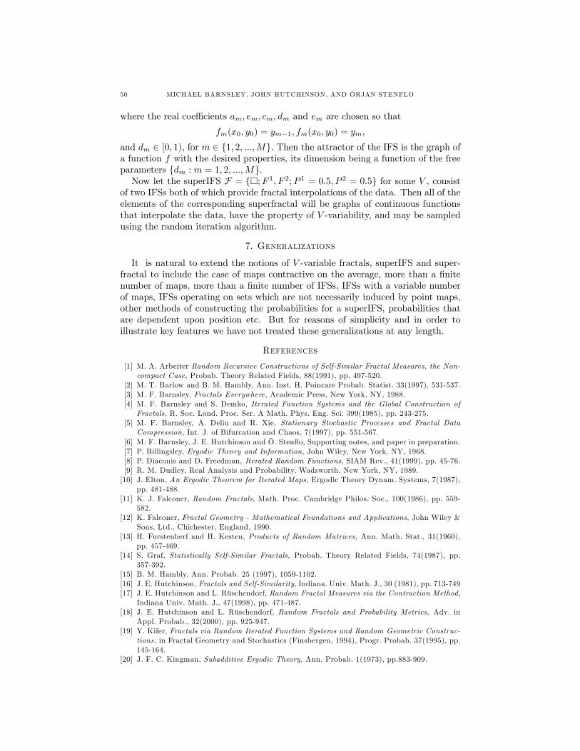
50 MICHAEL BARNSLEY, JOHN HUTCHINSON, AND ÖRJAN STENFLO
where the real coefficients am, em, cm, dm and em are chosen so that
fm(x0, y0) = ym−1, fm(x0, y0) = ym,
and dm ∈ [0, 1), for m ∈ 1, 2, ...,M. Then the attractor of the IFS is the graph ofa function f with the desired properties, its dimension being a function of the freeparameters dm : m = 1, 2, ...,M.Now let the superIFS F = ¤;F 1, F 2;P 1 = 0.5, P 2 = 0.5 for some V , consist
of two IFSs both of which provide fractal interpolations of the data. Then all of theelements of the corresponding superfractal will be graphs of continuous functionsthat interpolate the data, have the property of V -variability, and may be sampledusing the random iteration algorithm.
7. Generalizations
It is natural to extend the notions of V -variable fractals, superIFS and super-fractal to include the case of maps contractive on the average, more than a finitenumber of maps, more than a finite number of IFSs, IFSs with a variable numberof maps, IFSs operating on sets which are not necessarily induced by point maps,other methods of constructing the probabilities for a superIFS, probabilities thatare dependent upon position etc. But for reasons of simplicity and in order toillustrate key features we have not treated these generalizations at any length.
References
[1] M. A. Arbeiter Random Recursive Constructions of Self-Similar Fractal Measures, the Non-compact Case, Probab. Theory Related Fields, 88(1991), pp. 497-520.
[2] M. T. Barlow and B. M. Hambly, Ann. Inst. H. Poincare Probab. Statist. 33(1997), 531-537.[3] M. F. Barnsley, Fractals Everywhere, Academic Press, New York, NY, 1988.[4] M. F. Barnsley and S. Demko, Iterated Function Systems and the Global Construction of
Fractals, R. Soc. Lond. Proc. Ser. A Math. Phys. Eng. Sci. 399(1985), pp. 243-275.[5] M. F. Barnsley, A. Deliu and R. Xie, Stationary Stochastic Processes and Fractal Data
Compression, Int. J. of Bifurcation and Chaos, 7(1997), pp. 551-567.[6] M. F. Barnsley, J. E. Hutchinson and Ö. Stenflo, Supporting notes, and paper in preparation.[7] P. Billingsley, Ergodic Theory and Information, John Wiley, New York, NY, 1968.[8] P. Diaconis and D. Freedman, Iterated Random Functions, SIAM Rev., 41(1999), pp. 45-76.[9] R. M. Dudley, Real Analysis and Probability, Wadsworth, New York, NY, 1989.[10] J. Elton, An Ergodic Theorem for Iterated Maps, Ergodic Theory Dynam. Systems, 7(1987),
pp. 481-488.[11] K. J. Falconer, Random Fractals, Math. Proc. Cambridge Philos. Soc., 100(1986), pp. 559-
582.[12] K. Falconer, Fractal Geometry - Mathematical Foundations and Applications, John Wiley &
Sons, Ltd., Chichester, England, 1990.[13] H. Furstenberf and H. Kesten, Products of Random Matrices, Ann. Math. Stat., 31(1960),
pp. 457-469.[14] S. Graf, Statistically Self-Similar Fractals, Probab. Theory Related Fields, 74(1987), pp.
357-392.[15] B. M. Hambly, Ann. Probab. 25 (1997), 1059-1102.[16] J. E. Hutchinson, Fractals and Self-Similarity, Indiana. Univ. Math. J., 30 (1981), pp. 713-749[17] J. E. Hutchinson and L. Rüschendorf, Random Fractal Measures via the Contraction Method,
Indiana Univ. Math. J., 47(1998), pp. 471-487.[18] J. E. Hutchinson and L. Rüschendorf, Random Fractals and Probability Metrics, Adv. in
Appl. Probab., 32(2000), pp. 925-947.[19] Y. Kifer, Fractals via Random Iterated Function Systems and Random Geometric Construc-
tions, in Fractal Geometry and Stochastics (Finsbergen, 1994), Progr. Probab. 37(1995), pp.145-164.
[20] J. F. C. Kingman, Subadditive Ergodic Theory, Ann. Probab. 1(1973), pp.883-909.
RANDOM IFSS 51
[21] R. D. Mauldin and S. C. Williams, Random Recursive Constructions; Asymptotic Geomet-rical and Topological Properties, Trans. Amer. Math. Soc., 295(1986), pp. 325-346.
[22] P. A. P. Moran, Additive Functions of Intervals and Hausdorff Measure, Proc. CambridgePhilos. Soc., 42(1946), pp.15-23.
[23] L. Olsen, Random Geometrically Graph Directed Self-Similar Multifractals, Pitman ResearchNotes, 307(1994), Longman, Harlow.
[24] N. Patzschke and U. Zähle, Self-Similar Random Measures. IV. The Recursive ConstructionModel of Falconer, Graf, and Mauldin and Williams, Math. Nachr. 149(1990), pp. 285-302.
[25] M. Peruggia, Discrete Iterated Function Systems, A. K. Peters, Wellesley, MA, 1993.[26] H. Sagan, Space-Filling Curves, Springer-Verlag, New York, N.Y., 1994.[27] Ö. Stenflo, Markov Chains in Random Environments and Random Iterated Function Sys-
tems, Trans. Amer. Math. Soc. 353(2001), 3547-3562.[28] U. Zähle, Self-Similar Random Measures. I. Notion, Carrying Hausdorff Dimension, and
Hyperbolic Distribution, Probab. Theory Related Fields, 80(1988), pp. 79-100.
335 Pennbrooke Trace, Duluth,, GA 30097, USAE-mail address : [email protected]
Department of Mathematics, Australian National UniversityE-mail address : [email protected]
Department of Mathematics, Stockholm University, SE-10691 Stockholm, SwedenE-mail address : [email protected]


![FRACTAL KOCH MULTIBAND TEXTILE ANTENNA … · Koch fractal antenna is able to reduce size up to 7% for flrst iteration and up to 26% for series iteration [19]. Koch fractal-slotted](https://img.pdfslide.us/doc/110x75/5fb1830efc40811fac69fceb/fractal-koch-multiband-textile-antenna-koch-fractal-antenna-is-able-to-reduce-size.jpg)