A FORWARD/REVERSE AUCTION ALGORITHM FOR ASYMMETRIC ...dimitrib/For_Rev_Asym_Auction.pdf · January 1993 LIDS-P-2159 A FORWARD/REVERSE AUCTION ALGORITHM FOR ASYMMETRIC ASSIGNMENT PROBLEMS

January 1993 LIDS-P-2159

A FORWARD/REVERSE AUCTION ALGORITHM

FOR ASYMMETRIC ASSIGNMENT PROBLEMS1

by

Dimitri P. Bertsekas2 and David A. Castanon3

Abstract

In this paper we consider the asymmetric assignment problem and we propose a new auction algorithm

for its solution. The algorithm uses in a novel way the recently proposed idea of reverse auction, where in

addition to persons bidding for objects by raising their prices, we also have objects competing for persons by

essentially offering discounts. In practice, the new algorithm apparently deals better with price wars than the

currently existing auction algorithms. As a result it frequently does not require ε-scaling for good practical

performance, and tends to terminate substantially (and often dramatically) faster than its competitors.

1 This work was supported in part by NSF under Grant CCR-9108058, and in part by the BM/C3 Technol-

ogy branch of the United States Army Strategic Defense Command. It will be published also by the Journal

of Computational Optimization and its Applications.2 Department of Electrical Engineering and Computer Science, M. I. T., Cambridge, Mass., 02139.3 Department of Electrical Engineering, Boston University, and ALPHATECH, Inc., Burlington, Mass.,

01803.

1

1. Introduction

1. INTRODUCTION

We consider the classical asymmetric assignment problem where we want to match m persons

with m out of n objects (m < n). The benefit for matching a person with an object is given, and

we want to assign all the persons to distinct objects so as to maximize the total benefit. There

are a number of methods for solving this problem, including primal-simplex and primal-dual (or

sequential shortest path) methods [Ber91], [KeH80], [PaS82], [Roc84]. In this paper we will focus

on auction algorithms, first proposed in [Ber79] for both symmetric and asymmetric problems, and

subsequently developed in several other papers [Ber85], [Ber88], [BeE88], [BCT91]. The textbook

[Ber91] contains an extensive discussion of these methods and their extensions to other network

flow problems. Recent experimental evidence suggests that auction algorithms outperform their

competitors by a substantial margin, particularly for sparse assignment problems [BeE88], [Ber90],

[BCT91], and are also well suited for parallel computation [BeC89], [KKZ90], [PhZ88], [WeZ90],

[WeZ91], [Zak91].

In the original proposal of the auction algorithm there is a price for each object, and at each

iteration, one or more unassigned persons bid simultaneously for their “best” objects (the ones

offering maximum benefit minus price), thereby raising the corresponding prices. Objects are then

awarded to the highest bidder. The bidding increments must be at least equal to a positive parameter

ε, and are chosen so as to preserve an ε-complementary slackness condition. For good practical (as

well as theoretical) performance, it may be important to use ε-scaling, which consists of applying the

algorithm several times, starting with a large value of ε and successively reducing ε up to an ultimate

value that is less than some threshold (1/m when aij are integer). Each scaling phase provides good

initial prices for the next. The original proposal of the auction algorithm for asymmetric assignment

problems had a deficiency: it required that the initial object prices be zero, thereby precluding

the use of ε-scaling. As a result the method was susceptible to “price wars”, that is, protracted

sequences of small price rises resulting from groups of persons competing for a smaller number of

roughly equally desirable objects. Thus, in order to use auction algorithms to solve asymmetric

problems where price wars are likely, one had to convert the problem to a symmetric one by adding

n − m artificial persons that can be assigned to any object at zero cost. There are specialized

versions of the auction algorithm (the auction algorithm with similar persons [BeC89]) that can take

advantage of the structure induced by the artificial persons. However, the approach of converting

the problem to a symmetric problem introduces an undesirable increase in the problem’s dimension

and to our knowledge has not seen much use.

In part to address the difficulty with price wars of the original asymmetric auction algorithm,

2

2. Asymmetric Assignment Problems

an alternative algorithm, called reverse auction, was recently developed in [BCT91]. Here, roughly

speaking, the objects compete for persons by lowering their prices. In particular, objects decrease

their prices to a level that is sufficiently low to lure a person away from its currently held object. One

can show that forward and reverse auctions are mathematically equivalent, but their combination has

resulted in algorithms that can solve various assignment-like problems much faster than forward or

reverse auction can by themselves. In particular, an ε-scaled version of a combined forward/reverse

auction was developed for asymmetric problems that can deal effectively with price wars. This

method operates principally as a forward auction and uses reverse auction only near the end to

rectify violations in the optimality conditions. According to computational results given in [BCT91],

the solution times of this method for m× n asymmetric problems are quite reasonable and do not

exceed the solution times of the original (forward only) auction algorithm for similar symmetric

m×m problems by a factor larger than the natural ratio n/m.

However, as demonstrated in [BCT91], by frequently switching between forward and reverse

auction, a substantial performance improvement can be obtained for symmetric assignment problems.

A natural question therefore arises whether a similar improvement can be realized for asymmetric

assignment problems by similarly combining forward and reverse auctions. The purpose of this paper

is to develop such a method. Contrary to the method given in [BCT91], it is typically unnecessary

to resort to ε-scaling, involving the solution of several subproblems, to deal with price wars. Our

computational results show that ...

In Section 2, we define the asymmetric assignment problem, and we develop ε-complementary

slackness conditions in a form suitable for our purposes. In Section 3, we introduce the new combined

forward/reverse auction algorithm and we develop its basic properties. Finally, in Section 4 we

provide computational results.

2. ASYMMETRIC ASSIGNMENT PROBLEMS

In the asymmetric assignment problem there are m persons and n objects (m < n). The benefit

or value for assigning person i to object j is aij . The set of arcs of the underlying bipartite graph is

denoted by AA = {(i, j) | j ∈ A(i), i = 1, . . . ,m}.

The set of objects to which person i can be assigned is a nonempty set denoted A(i). The set of

persons to which object j can be assigned is assumed nonempty and is denoted by B(j) = {i | j ∈A(i)}. An assignment S is a (possibly empty) set of person-object pairs (i, j) such that j ∈ A(i)

3

3. A Forward/Reverse Auction Algorithm for Asymmetric Assignment Problems

for all (i, j) ∈ S; for each person i there can be at most one pair (i, j) ∈ S; and for every object j

there can be at most one pair (i, j) ∈ S. Given an assignment S, we say that person i is assigned if

there exists a pair (i, j) ∈ S; otherwise we say that i is unassigned . We use similar terminology for

objects. An assignment is said to be feasible if it contains m pairs, so that every person is assigned;

otherwise the assignment is called partial . The problem is said to be feasible if there exists at least

one feasible assignment. We want to find an assignment{(1, j1), . . . , (m, jm)

}with maximum total

benefit∑m

i=1 aiji .

A dual problem can be defined by introducing a price variable pj for each object j and a profit

variable πi for each person i. It was shown in [BCT91] (see also [Ber91]) that a corresponding dual

problem is

minimize

m∑

i=1

πi +

n∑

j=1

pj − (n−m) minj=1,...,n

pj

subject to πi + pj ≥ aij , ∀ (i, j) ∈ A. (1)

We denote by p the vector of prices (p1, . . . , pn), and by π the vector of profits (π1, . . . , πm). The

following condition was introduced in [BCT91] for an assignment S and a pair (π, p).

Definition 1: An assignment S and a pair (π, p) are said to satisfy ε-complementary slackness

(ε-CS for short) if

πi + pj ≥ aij − ε, ∀ (i, j) ∈ A, (2a)

πi + pj = aij, ∀ (i, j) ∈ S, (2b)

pj ≤ mink: assigned under S

pk, ∀ j : unassigned under S. (2c)

The following proposition, proved in [BCT91], clarifies the significance of ε-CS.

Proposition 1: If a feasible assignment S satisfies the ε-CS conditions (2a)-(2c) together with

a pair (π, p), then S is within mε of being optimal for the asymmetric assignment problem. In

particular, if the benefits aij are all integer and ε < 1/m, S is an optimal assignment.

3. A FORWARD/REVERSE AUCTION ALGORITHM FOR ASYMMETRIC ASSIGNMENT

PROBLEMS

In this section we consider algorithms that use a fixed ε > 0, and maintain an assignment S and a

pair (π, p) satisfying together with S the first two ε-CS conditions (2a) and (2b). They also maintain

a scalar λ such that

pj ≥ λ, ∀ j that are assigned under S. (3)

4


The algorithms terminate when S becomes feasible and in addition all unassigned objects j satisfy

pj ≤ λ. Thus upon termination, in view of Eq. (3), the third ε-CS condition (2c) is satisfied and by

Prop. 1, the assignment S is optimal if ε < 1/m and the benefits aij are all integer. The level λ may

be viewed as a profitability threshold below which we cannot drop the price of any assigned object.

In the course of the algorithm, λ may be adjusted downward if it is set initially so high that not all

persons can be assigned at prices above λ.

Note that we can initially select S to be empty, λ and p to be arbitrary, and πi to be sufficiently

large so that the conditions (2a) and (2b) are satisfied. Thus, in particular, we can try to use a

favorable price vector such as one obtained from a scaling phase corresponding to a larger value of

ε.

3.1 Forward and Reverse Auction Iterations

There are two types of iterations, forward and reverse. Forward iterations can be performed only as

long as there is an unassigned person and reverse iterations can be performed only as long as there

is an unassigned object j with pj > λ. Both types of iterations start with an assignment S, a pair

(π, p), and a scalar λ satisfying conditions (2a), (2b), and (3).

Forward Iteration

Find an unassigned person i, its best object ji

ji = arg maxj∈A(i)

{aij − pj}, (4)

the corresponding values

vi = maxj∈A(i)

{aij − pj}, (5)

and

wi = maxj∈A(i),j 6=ji

{aij − pj}. (6)

[If ji is the only object in A(i), we define wi to be −∞ or, for computational purposes, a number that is

much smaller than vi.] Set

pji := max{λ, aiji − wi + ε}, (7)

πi := wi − ε. (8)

If λ ≤ aiji −wi + ε, add (i, ji) to S and if ji was assigned to some i′ at the start of the iteration, remove

from S the pair (i′, ji).

5


Reverse Iteration

Find an unassigned object j with pj > λ, its best person ij

ij = arg maxi∈B(j)

{aij − πi}, (9)

the corresponding values

βj = maxi∈B(j)

{aij − πi}, (10)

and

γj = maxi∈B(j),i 6=ij

{aij − πi}. (11)

[If ij is the only object in B(j), we define γj to be ∞ or, for computational purposes, a number that is

much larger than βj .] Proceed according to the following two cases:

(1) βj ≥ λ + ε. In this case set

pj := max{λ, γj − ε}, (12)

πij := aij j −max{λ, γj − ε}, (13)

add (ij , j) to S, and if ij was assigned to some j ′ at the start of the iteration, remove from S the pair

(ij , j′).

(2) βj < λ + ε. In this case, set

pj := βj − ε (14)

and if the number of objects k with pk < λ is now more than n−m, set λ to the value

min{ξ | pk ≤ ξ for n−m or more objects k}. (15)

Note that λ remains unchanged in a forward iteration, and it can either decrease or stay unchanged

in a reverse iteration. Note also that the “bidding object” j in the reverse iteration may not be

assigned during the iteration; this happens when its “best value” βj is low relative to λ, in which

case its price pj is reduced below λ [cf. Eq. (14)], and the object cannot bid again until λ decreases

from its current level. Figure 1 illustrates the two cases that can arise in the reverse iteration.

The next proposition establishes a basic property of the forward and reverse iterations:

Proposition 2: Suppose that at the beginning of a forward or a reverse iteration, (π, p) satisfies

together with S the first two ε-CS conditions (2a) and (2b), and λ satisfies condition (3). The same

is true for (π, p), S, and λ at the end of the iteration.

Proof: Suppose that the iteration starts with S, (π, p), and λ satisfying Eqs. (2a), (2b), and (3).

Let S, (π, p), and λ be the corresponding quantities at the end of the iteration.

6


εεελ + ε

λ

λ + ελ + ε

λλ

(a) (b) (c)

β j

γ − εj

jp jpjp

β j

β jγ

j

γj

β − εj

Price change of object j



Object j gets assigned

Object j remains unassigned

Object j gets assigned

Figure 1: Illustration of the possible cases that can arise in the reverse iteration. These are:

(a) βj ≥ λ+ ε and γj − ε > λ. Then j gets assigned to ij , pj is set to γj − ε, and πij is set to aij j −γj + ε.

(b) βj ≥ λ + ε and γj − ε ≤ λ. Then j gets assigned to ij , pj is set to λ, and πij is set to aij j − λ.

(c) βj < λ + ε. Then j stays unassigned and pj is set to βj − ε, while πij remains unchanged.

Consider first a forward iteration and let i be the corresponding unassigned person that submits

the bid as per Eqs. (4)-(8). We will first verify that the pair (π, p) satisfies Eq. (2a) for each arc.

From Eqs. (4)-(6), we see that aiji −wi ≥ pji , so by Eq. (7), we have

pji≥ pji + ε. (16)

By adding this relation to the relation πk + pji ≥ akji− ε [cf. Eq. (2a)], and by using the fact πk = πk

for all k 6= ij , we obtain

πk + pji≥ akji − ε, ∀ k ∈ B(ji), k 6= i. (17)

On the other hand, since pj = pj for all j 6= ji, we have

πi = wi − ε ≥ aij − pj − ε = aij − pj − ε, ∀ j ∈ A(i), j 6= ji,

while from Eqs. (7) and (8), we have

πi = wi − ε ≥ aiji − pji − ε.

Combining the last two relations, we obtain

πi + pj ≥ aij − ε, ∀ j ∈ A(i). (18)

7


Finally, for arcs (k, j) with k 6= i, j 6= ji, we have πk = πk and pj = pj , so by Eq. (2a), we obtain

πk + pj ≥ akj − ε, ∀ (k, j) ∈ A, k 6= i, j 6= ji. (19)

By combining Eqs. (17)-(19), we see that

πk + pj ≥ akj − ε, ∀ (k, j) ∈ A,

that is, the ε-CS condition (2a) holds at the end of the iteration.

We next show that Eq. (2b) is preserved by the iteration, that is,

πk + pj = akj , ∀ (k, j) ∈ S. (20)

Note that if (k, j) ∈ S and j 6= ji, we must have k 6= i, (k, j) ∈ S, and πk = πk, pj = pj , so by using

the hypothesis [cf. Eq. (2b)], we see that Eq. (20) holds. If on the other hand (k, ji) ∈ S for some k,

we claim that k = i, since otherwise, by the rules of the iteration, we would have λ > aiji − wi + ε,

so that by Eqs. (7) and (16),

λ = pji≥ pji + ε,

contradicting the condition (3). Now if (i, ji) ∈ S, we must have by the rules of the iteration,

λ ≤ aiji − wi + ε and pji= aiji − wi + ε, so that

πi = wi − ε = aiji − pji. (21)

We see therefore that Eq. (20) holds for the case where j = ji as well.

Finally, to show that condition (3) is preserved by the iteration, note that λ = λ, that pj = pj for

all j 6= ji, and that pji≥ λ [cf. Eq. (7)]. Since the only object that can become assigned during the

iteration is ji, we see that

pj ≥ λ, ∀ j that are assigned under S.

The proof of the proposition for the case of a forward iteration is thus complete.

Consider next the case of a reverse iteration. Let j be the corresponding unassigned object that

submits the bid as per Eqs. (9)-(13).

In the case where βj ≥ λ + ε, we have by Eqs. (12) and (13)

πij = aijj −max{λ, γj − ε} ≥ aijj − βj + ε = πij + ε if βj ≥ λ + ε. (22)

By using also the relation πij + pj ≥ aijj − ε, we have

pj = max{λ, γj − ε} ≤ βj − ε = aijj − πij − ε ≤ pj if βj ≥ λ + ε. (23)

8


In the case where βj < λ+ ε we have γj ≤ βj < λ− ε and by using also the fact pj > λ, we obtain

pj = βj − ε < λ < pj if βj < λ + ε, (24)

πij = πij if βj < λ + ε. (25)

To prove that the ε-CS condition (2a) is preserved by the reverse iteration, consider first the arcs

(i, j) with i 6= ij . Since πi = πi and pj ≥ γj − ε, we have

πi + pj ≥ πi + γj − ε ≥ πi + aij − πi − ε = aij − ε, ∀ i ∈ B(j), i 6= ij . (26)

Consider next the arcs (ij , k) with k 6= j. We have πij + pk ≥ aijk− ε [cf. Eq. (2a)], and since pk = pk

for k 6= j, we obtain [cf. Eq. (22)]

πij + pk ≥ πij + ε + pk ≥ aijk if βj ≥ λ + ε, k 6= j, (27)

and [cf. Eq. (25)]

πij + pk = πij + pk ≥ aijk − ε if βj < λ + ε, k 6= j. (28)

Finally for the arc (ij , j), we have by Eq. (13),

πij + pj = aijk if βj ≥ λ + ε, (29)

and by Eq. (14),

πij + pj = πij + βj − ε = aijj − ε if βj < λ + ε. (30)

By combining Eqs. (26)-(30), we see that

πi + pk ≥ aik − ε, ∀ (i, k) ∈ A,

so the condition (2a) is preserved by the reverse iteration.

To show that Eq. (2b) is preserved by the reverse iteration, that is,

πi + pk = aik, ∀ (i, k) ∈ S, (31)

note that if (i, k) ∈ S and i 6= ij , we must have πi = πi, pk = pk, and (i, k) ∈ S, so by using the

hypothesis [cf. Eq. (2b)], we see that Eq. (31) holds. If on the other hand (ij , k) ∈ S for some k,

then either k = j in which case we must have πij + pj = aijj by Eqs. (12) and (13), or else k 6= j, in

which case (ij , k) ∈ S, πij = πij , and pk = pk , so by Eq. (2b) and the induction hypothesis we have

9


πij + pk = aijk . Thus Eq. (31) holds in all cases and the condition (2b) is preserved by the reverse

iteration.

Finally to show that Eq. (3) is preserved by the reverse iteration, note that λ ≥ λ, while the only

object that can become assigned during the iteration and whose price can change is j. On the other

hand if j becomes assigned, we must have pj ≥ λ by Eq. (12), so at the end of the iteration, we will

have pj ≥ λ, thereby preserving Eq. (3). Q.E.D.

As a corollary of the preceding proof, we obtain the following proposition.

Proposition 3: Suppose that S, (π, p), and λ satisfy conditions (2a), (2b), and (3). Then:

(a) In a forward iteration, pji increases by at least ε. Furthermore, either ji is assigned to i

during the iteration and pji is increased to a level no less than λ, or else pji is increased to

the level λ.

(b) In a reverse iteration, either πij increases by at least ε and j becomes assigned, or else j

remains unassigned and pj decreases to a level below λ.

(c) If all persons are assigned (S is feasible), the reverse iteration leaves λ unchanged.

Proof: (a) See Eqs. (7) and (16).

(b) See Eqs. (22) and (24).

(c) If all persons are assigned, the number of assigned objects k is m and all these objects satisfy

pk ≥ λ by Eq. (3). Therefore, the number of objects k with pk < λ cannot become more than n−m,

which is the only situation where λ can change. Q.E.D.

We will now use the results obtained so far to analyse several possible algorithms.

3.2 Purely Forward Algorithm

It is possible to consider a forward auction algorithm that consists exclusively of forward iterations.

In such an algorithm it is essential to choose initially λ ≥ pj for all unassigned objects j. Then, since

λ will remain unchanged, by using Prop. 3(a), it can be seen that in the course of the algorithm, we

will have

maxk: unassigned under S

pk ≤ λ ≤ mink: assigned under S

pk , ∀ j : unassigned under S, (32)

so by using also Prop. 2, we see that all three ε-CS conditions (2a)-(2c) will be satisfied. Furthermore,

by Prop. 3(a), the price pji is increased by at least ε at each forward iteration. Using this fact and

10


standard arguments (see e.g. [Ber88], [Ber91]), it can be shown that this forward algorithm will

terminate with a feasible assignment S that satisfies ε-CS together with (π, p) (and is optimal if

ε < 1/m and the problem data are integer). Unfortunately, even though this forward algorithm will

work with arbitrary initial prices, it is not suitable for use in conjunction with ε-scaling because of

the initial requirement that λ ≥ pj for all unassigned objects j. Since for an object to get assigned

its price must rise to at least the level λ, the advantage of approximately optimal initial prices that

ε-scaling attempts to carry from one ε-scaling phase to the next is largely diminished.

3.3 Purely Reverse Algorithm

It is also possible to consider a purely reverse auction algorithm that consists exclusively of reverse

iterations, provided that the initial assignment is feasible and the initial λ is such that condition (3)

is satisfied (λ ≥ pj for all assigned objects j). The following proposition establishes the validity of

the algorithm.

Proposition 4: For a feasible problem, the purely reverse algorithm starting from a feasible

assignment, a pair (π, p), and a scalar λ satisfying conditions (2a), (2b), and (3) terminates. The

assignment obtained satisfies ε-CS together with (π, p).

Proof: From Prop. 3(c), we have that λ will remain unchanged and that at each iteration there are

two possibilities: (1) πij will increase by ε and the selected unassigned object j will get assigned to

ij , or (2) The number of unassigned objects whose price exceeds λ will decrease by one. Therefore,

after some iteration, case (1) will occur exclusively. By Eq. (13) we have

πij = aijj −max{λ, γj − ε} ≤ aijj − λ, (33)

so πij cannot exceed max(i,k)∈A aik − λ. It follows that the algorithm cannot execute an infinite

number of iterations and must therefore terminate. Q.E.D.

The disadvantage of the purely reverse algorithm is that it requires an initial feasible assignment.

The reason is that if the current assignment S is infeasible, we may have pj ≤ λ for all unassigned

objects j, while we have pj < λ for no more than n − m unassigned objects. Then the purely

reverse algorithm will leave λ unchanged and will terminate without finding a feasible solution. A

possible remedy is to start with an arbitrary assignment but to reduce λ by some positive increment

whenever the difficulty just described occurs. Unfortunately, however, it is not easy to determine

the proper size of the increment for fast termination.

Another possibility to circumvent the need for an initial feasible assignment is to combine the

forward and reverse algorithms, so that the forward part guarantees that a feasible assignment will

11


be obtained, while the reverse part is capable of dealing with essentially arbitrary starting values

of λ. In particular, one may use the purely forward algorithm first to obtain a feasible assignment,

and then switch to the reverse algorithm after setting

λ = mink: assigned under S

.

This is the algorithm proposed in [BCT91]; it is suitable for ε-scaling but does not take advantage

of the beneficial effect of mixing the forward and the reverse algorithms that was demonstrated for

symmetric problems in [BCT91]. The following algorithm switches several times between the two

algorithms aiming at less reliance on ε-scaling and faster termination.

3.4 Combined Forward/Reverse Algorithm

The combined forward/reverse algorithm that we now introduce switches between forward and

reverse auction until all persons are assigned. Then it executes reverse iterations exclusively, aiming

to satisfy the final remaining optimality condition (pj ≤ λ for all unassigned objects j). The initial

S, (π, p), and λ must satisfy the ε-CS conditions (2a), (2b), and the condition λ ≤ pj for all assigned

objects j. Thus if the initial assignment is empty, any initial p and λ can be used. We assume

that initially there is at least one unassigned person (otherwise the forward part of the algorithm is

inapplicable and unnecessary).

Combined Forward/Reverse Auction Algorithm

Step 1: (Forward auction cycle) Execute iterations of the forward auction algorithm until at least

one more person becomes assigned. If there is an unassigned person left, go to Step 2; else go to Step 3.

Step 2: (Reverse auction cycle) Execute several iterations of the reverse auction algorithm until at

least one more object becomes assigned or until we have pj ≤ λ for all unassigned objects j. If there is

an unassigned person left, go to Step 1; else go to Step 3.

Step 3: (Reverse auction) Execute successive iterations of the reverse auction algorithm until the

algorithm terminates with pj ≤ λ for all unassigned objects j.

The following proposition establishes the validity of the algorithm.

Proposition 5: For a feasible problem, the combined forward/reverse algorithm terminates with

an optimal assignment.

Proof: We will assume that the algorithm does not terminate and will arrive at a contradiction.

When the algorithm obtains a feasible assignment, it gets reduced to the purely reverse algorithm

and terminates by Prop. 4. Assume therefore that the algorithm never obtains a feasible assignment.

12


Since the cardinality of the assignment must increase before switching from a forward to a reverse

cycle, there are two possibilities: (1) The algorithm will execute forward iterations exclusively after

some iteration, or (2) The algorithm will execute reverse iterations exclusively after some iteration,

and we will always have pj > λ for some unassigned object j.

In case (1) the algorithm will be reduced to the purely forward algorithm, and as discussed earlier,

it must terminate for a feasible problem. This contradicts our earlier hypothesis that the algorithm

does not terminate.

In case (2), since whenever a profit variable increases it increases by at least ε, there are two

possibilities:

(a) After some iteration, all πi stay constant and no object changes assignment.

(b) Some profit variable increases to ∞, in which case by the argument given in the proof of

Prop. 4 [cf. Eq. (33)], λ decreases to −∞.

In case (a), the variables βj stay constant after some iteration, so in view of Eq. (14), the object

prices cannot change after some iteration. This contradicts Prop. 3(b), which states that pj < pj at

each reverse iteration [see also Eq. (24)].

In case (b), let

J∞ = {j | pj → −∞}, J∞ = {j | j /∈ J∞},

I∞ = {i | πi →∞}, I∞ = {i | i /∈ I∞}.

By the ε-CS condition (2a), we must have

i ∈ I∞ ⇒ j ∈ J∞ ∀ (i, j) ∈ A, (34)

i ∈ I∞ ⇒ j ∈ J∞ ∀ (i, j) ∈ A. (35)

We claim that after some iteration, each of the objects in J∞ must be assigned at all times to

the same person from I∞. To see this, note that if some object j ∈ J∞ bids an infinite number of

times for some person ij , then πij will increase by at least ε an infinite number of times, in view of

Prop. 3(b), the definition of J∞, and the fact λ → −∞. On the other hand by Eq. (35), we must

have ij ∈ I∞, so πij must remain bounded and we have a contradiction.

Thus, I∞ contains the set of persons that are assigned to J∞ plus the nonempty set of persons

that are unassigned throughout the last reverse cycle (a person that becomes assigned in a reverse

cycle remains assigned for the duration of the cycle). Therefore, the number of persons in I∞ exceeds

the number of objects in J∞. In view of Eq. (35), this contradicts the hypothesis that the problem

is feasible. Q.E.D.

13


A careful examination of the preceding proof shows that there are other valid variations of the

combined/forward reverse algorithm, corresponding to variations of the reverse iterations and/or

the scheme for switching from a reverse to a forward cycle. What is important is that: (a) λ should

remain unchanged at all forward iterations and at all reverse iterations where the current assignment

is feasible, (b) λ should not increase during all reverse iterations (again here only unassigned objects

j with pj > λ should be allowed to bid), and (c) a mechanism is provided whereby the combined

method is guaranteed to eventually exit from a reverse cycle if the current assignment is not feasible.

Consider now what happens if the problem is infeasible. Then, eventually the number of unas-

signed persons will stop decreasing and the method will get caught in either a forward cycle (Step

1) or in a reverse cycle (Step 2). Infeasibility will then be detected in the standard way for auction

algorithms, that is, some price or some profit will exceed a certain precomputable upper bound, as

described in [Ber91]. It is also possible to deal with infeasibility by adding a sufficient number of

artificial arcs to convert the problem to a feasible problem. These arcs must have sufficiently small

values to guarantee that they are not part of an optimal assignment unless the original problem is

infeasible; see [Ber91].

3.5 An Alternative Reverse Iteration and Combined Forward/Reverse Algorithm

A variation of the reverse iteration is obtained if we keep λ constant, even if the number of

objects k with pk < λ becomes greater than n−m. Thus, this alternative iteration is defined to be

identical to the one given earlier except that we forego the change of λ in case (2) [cf. Eq. (15)]. For

this iteration, Props. 2 and 3 still hold, but the purely reverse algorithm may terminate with some

persons still unassigned because λ was set to a value so high that the number of unassigned objects

with price less or equal to λ exceeds n−m. Nonetheless, if the alternative iteration is combined with

the forward iteration as in the algorithm given earlier, the resulting combination is valid because

forward iterations will continue as long as there are some unassigned persons, even if no reverse

iterations can be executed.

Note that λ remains unchanged throughout this alternative combined forward/reverse algorithm,

and can only change at the beginning of each scaling phase. Thus, the choice of λ at each scaling

phase is critical for the algorithm’s performance. A reasonable scheme is to choose λ at the beginning

of each scaling phase except the first as

λ = minj: assigned under S

pj ,

where S is the assignment obtained at the end of the preceding scaling phase. At the first scaling

phase one may start with the empty assignment, zero object prices, and λ = 0. With these choices,

14

4. Computational Results

no reverse iterations will be executed in the first scaling phase, since the prices of the unassigned

objects as well as λ will remain at zero throughout the phase.

4. COMPUTATIONAL RESULTS

In order to evaluate the relative performance of the new forward/reverse auction algorithms, we

implemented both variations of the combined forward-reverse auction algorithms discussed previ-

ously and the auction algorithm for inequality constraints from [ BCT91]. The three algorithms

were evaluated on the following classes of inequality-constrained assignment problems:

1. Randomly generated problems, generated using the DIMACS assign.c problem generator [Cas92],

which also include a number of high-cost arcs.

2. Geometric matching problems, consisting of matching a list of two-dimensional points with a

randomly-perturbed copy of the same list.

3. Clustered geometric matching problems, consisting of matching a list of clustered two-dimensional

points with a randomly perturbed copy of the same list.

The last two classes are representative of an important class of applications which motivated this

research: data association in multi-object tracking. In these problems, new sensor measurements

at each time frame must be associated with the predicted p osition of existing tracks. Due to the

presence of false alarms (due to clutter or other effects), missed detections and sensor measurement

inaccuracies, the set of measurement values will be a random perturbation of the set of predicted

positions. The maximum likelihood problem of determining which measurement-track associations

are most likely is equivalent to an inequality-constrained assignment problem.

4.1 Results on Random Problems

Table 1 summarizes the results of our random experiments for inequality-constrained assignment

problems with 2000 persons. In these experiments, an initial random problem is generated with 8

arcs per person, with cost range [1,200]. Based on the results of [BCT91], purely random problems

are often easy to solve and require no scaling; in order to make scaling necessary, we modified the

problems to increase the costs of 20% of the arcs by a factor of 100. The resulting inequality-

constrained assignment problems have a difficult structure which requires scaled auction algorithms,

as discussed in [BCT91]. The AS algorithm is the forward-reverse algorithm of [BCT91] discussed

in Section 3.3, which uses a scaled forward auction algorithm to find a complet e assignment of

15


persons into objects and a set of dual prices satisfying conditons (2a), (2b) and (3), and then uses

a purely reverse algorithm to find an optimal assignment. The ASFR1 algorithm is the combined

forward-reverse algorithm of Section 3.4, a nd the ASFR2 is the combined forward-reverse algorithm

of Section 3.5.

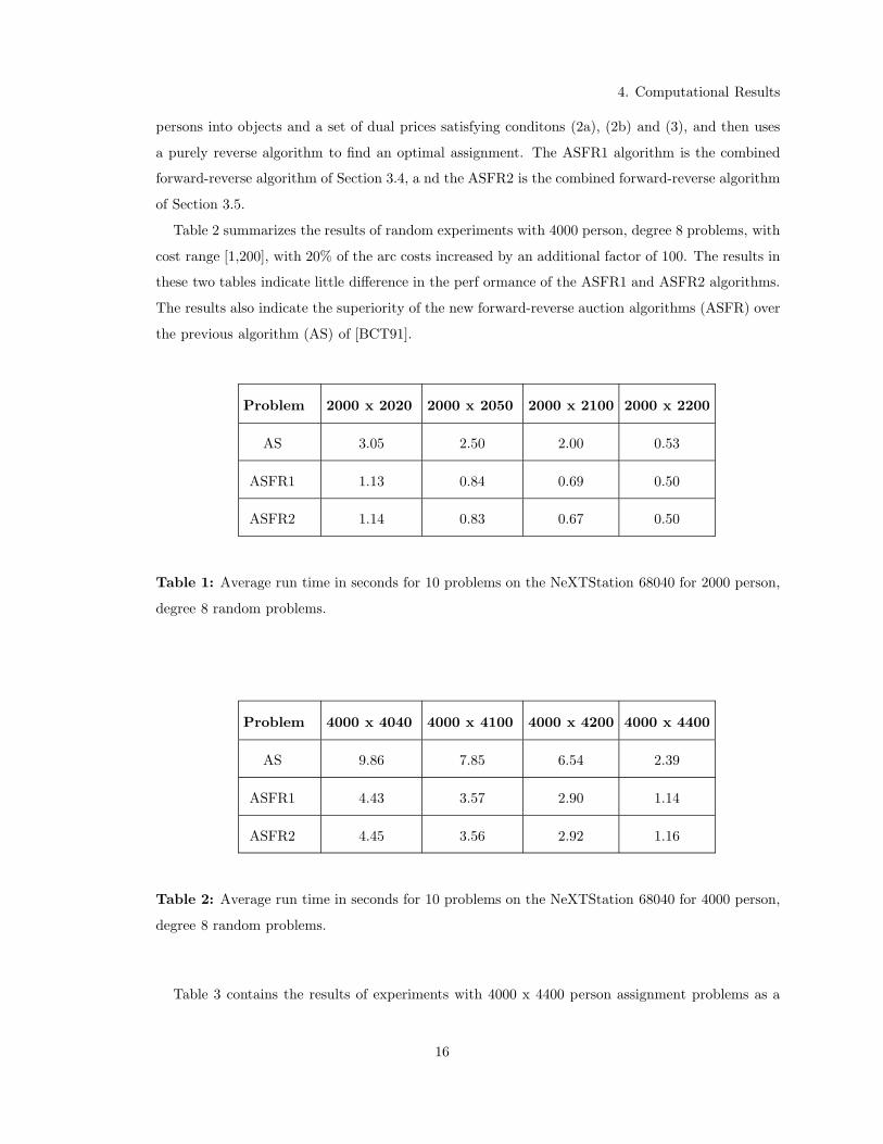
Table 2 summarizes the results of random experiments with 4000 person, degree 8 problems, with

cost range [1,200], with 20% of the arc costs increased by an additional factor of 100. The results in

these two tables indicate little difference in the perf ormance of the ASFR1 and ASFR2 algorithms.

The results also indicate the superiority of the new forward-reverse auction algorithms (ASFR) over

the previous algorithm (AS) of [BCT91].

Problem 2000 x 2020 2000 x 2050 2000 x 2100 2000 x 2200

AS 3.05 2.50 2.00 0.53

ASFR1 1.13 0.84 0.69 0.50

ASFR2 1.14 0.83 0.67 0.50

Table 1: Average run time in seconds for 10 problems on the NeXTStation 68040 for 2000 person,

degree 8 random problems.

Problem 4000 x 4040 4000 x 4100 4000 x 4200 4000 x 4400

AS 9.86 7.85 6.54 2.39

ASFR1 4.43 3.57 2.90 1.14

ASFR2 4.45 3.56 2.92 1.16

Table 2: Average run time in seconds for 10 problems on the NeXTStation 68040 for 4000 person,

degree 8 random problems.

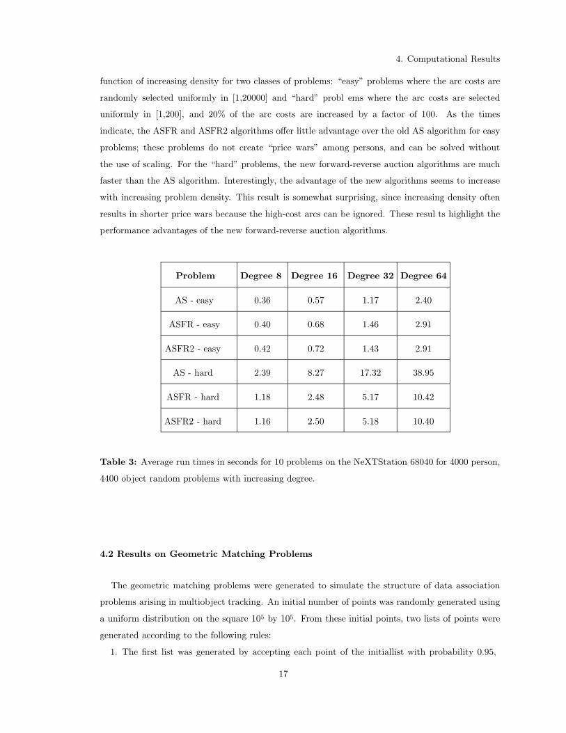
Table 3 contains the results of experiments with 4000 x 4400 person assignment problems as a

16


function of increasing density for two classes of problems: “easy” problems where the arc costs are

randomly selected uniformly in [1,20000] and “hard” probl ems where the arc costs are selected

uniformly in [1,200], and 20% of the arc costs are increased by a factor of 100. As the times

indicate, the ASFR and ASFR2 algorithms offer little advantage over the old AS algorithm for easy

problems; these problems do not create “price wars” among persons, and can be solved without

the use of scaling. For the “hard” problems, the new forward-reverse auction algorithms are much

faster than the AS algorithm. Interestingly, the advantage of the new algorithms seems to increase

with increasing problem density. This result is somewhat surprising, since increasing density often

results in shorter price wars because the high-cost arcs can be ignored. These resul ts highlight the

performance advantages of the new forward-reverse auction algorithms.

Problem Degree 8 Degree 16 Degree 32 Degree 64

AS - easy 0.36 0.57 1.17 2.40

ASFR - easy 0.40 0.68 1.46 2.91

ASFR2 - easy 0.42 0.72 1.43 2.91

AS - hard 2.39 8.27 17.32 38.95

ASFR - hard 1.18 2.48 5.17 10.42

ASFR2 - hard 1.16 2.50 5.18 10.40

Table 3: Average run times in seconds for 10 problems on the NeXTStation 68040 for 4000 person,

4400 object random problems with increasing degree.

4.2 Results on Geometric Matching Problems

The geometric matching problems were generated to simulate the structure of data association

problems arising in multiobject tracking. An initial number of points was randomly generated using

a uniform distribution on the square 105 by 105. From these initial points, two lists of points were

generated according to the following rules:

1. The first list was generated by accepting each point of the initial list with probability 0.95,

17


independent across points. This effect was chosen to simulate missed detections. Thus, the

first list is a reduction of the initial list of po ints.

2. The second list was generated by first accepting each point of the initial list with probability

0.95, independent across points and across the events used to generate the first list. This effect

was chosen to simulate false alarms in the data set. Then, the locations of all the points in

the second list were shifted by a constant bias, which was randomly generated from a bivariate

Gaussian distribution with a specified bias standard deviation. Subsequently, each point in the

second list was shifted by an independent bivariate Gaussian random variable, representing

measurement noise, with a specified measurement standard deviation.

3. The list with the least number of points was selected to be the persons in the inequality

assignment problem. The other list was selected to be the objects. Arcs were created between

each person-object pair for which the Euclidean distanc e between the corresponding points

was less than 3 times the measurement standard deviation. The costs assigned to each arc

were integers between 1 and 1000, proportional to the Euclidean distance of the corresponding

person-object pair.

4. In order to guarantee feasibility of the inequality assignment problem, an extra object node

was introduced for each person node, with a corresponding arc cost of 20000. This large cost

encouraged the problem to find a feasible assignment without using the extra nodes.

Table 4 summarizes our results with random geometric experiments corresponding to 2000 points

in the initial list. Four different combinations of bias/measurement standard deviation were tested.

For each combination, Table 4 lists the average run times across 10 different problems with similar

statistics for each of the three algorithms. For small bias/measurement standard deviations, the

points in the person lists and object lists are far appart, and thus the solution of the assignment

problem is triv ial. As the standard deviation increases, object-person groups form with an unbal-

anced number of persons or real objects in the group (because of the missed detection and false

alarm probability 0.95). This creates long price wars to determine which ext ra person in the group

will be assigned to an artificial object, or objects will remain unassigned. The size of these groups

increases with bias/measurement standard deviations, leading to longer price wars.

As the results in Table 4 indicate, the new forward-reverse algorithms are much more efficient than

the AS algorithm of [BCT91]. The reason for this efficiency is that forward and reverse iterations

are interleaved at each scaling step; in contrast, the AS algorithm performs only forward iterations

at most scales, and then switches to an unscaled reverse-only algorithm. Most of the computation

time (over 95 %) is spent in this unscaled reverse-only algorithm trying to enforce condition (2c) for

groups with more objects than persons. The new forward-reverse algorithms use scaling both for

forward and reverse iterations, resulting in more robust performance for this class of problems.

18


Bias/Measurement SD 5/50 10/100 15/150 20/200

AS 0.26 30.37 378.42 374.03

ASFR 0.32 1.67 3.78 9.34

ASFR2 0.34 1.62 3.04 5.99

Table 4: Average run times in seconds on the NeXTStation 68040 across 10 geometric problems

with 2000 points per list, probabilty of detection 0.95.

4.3 Results on Clustered Geometric Matching Problems

The clustered geometric matching problems were generated to simulate a different type of data

association problems arising in multiobject tracking: groups of objects moving close together, but

with significant distance among the groups. The principal dif ference between this class of problems

and the geometric class of problems is the location of the initial number of points, which are generated

as follows:

1. An initial number of cluster centers are generated with a uniform distribution on the square

105 by 105.

2. For each cluster center, a fixed number of points is generated by adding to the cluster center

an independent bivariate Gaussian random variable with a specified cluster spread standard

deviation.

Once the initial list of points is available, generation of the inequality constrained assignment problem

follows identically steps 1-5 of the geometric matching problems of the previous section.

Table 5 summarizes our results with random geometric experiments corresponding to 50 clusters of

40 points each in the initial list. Four different combinations of spread/measurement/bias standard

deviation were tested. For each combination, Table 5 li sts the average run times across 10 different

problems with similar statistics for each of the three algorithms. For small spread/measurement/bias

standard deviations, the assignment problem decouples by cluster, and thus corresponds to solution

of 50 sm all problems. As the spread standard deviation increases, the assignment problems become

coupled across clusters, and finding an optimal assignment becomes harder, and more susceptible to

long price wars.

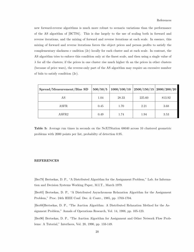
The results in Table 5 agree closely with the results from Table 4. The performance of the

19

References

new forward-reverse algorithms is much more robust to scenario variations than the performance

of the AS algorithm of [BCT91]. This is due largely to the use of scaling both in forward and

reverse iterations, and the mixing of forward and reverse iterations at each scale. In essence, this

mixing of forward and reverse iterations forces the object prices and person profits to satisfy the

complementary slackness c ondition (2c) locally for each cluster and at each scale. In contrast, the

AS algorithm tries to enforce this condition only at the finest scale, and then using a single value of

λ for all the clusters; if the prices in one cluster rise much higher th an the prices in other clusters

(because of price wars), the reverse-only part of the AS algorithm may require an excessive number

of bids to satisfy condition (2c).

Spread/Measurement/Bias SD 500/50/5 1000/100/10 2500/150/15 2000/200/20

AS 1.04 28.33 225.60 813.92

ASFR 0.45 1.70 2.21 3.68

ASFR2 0.49 1.74 1.94 3.53

Table 5: Average run times in seconds on the NeXTStation 68040 across 10 clustered geometric

problems with 2000 points per list, probabilty of detection 0.95.

REFERENCES

[Ber79] Bertsekas, D. P., “A Distributed Algorithm for the Assignment Problem,” Lab. for Informa-

tion and Decision Systems Working Paper, M.I.T., March 1979.

[Ber85] Bertsekas, D. P., “A Distributed Asynchronous Relaxation Algorithm for the Assignment

Problem,” Proc. 24th IEEE Conf. Dec. & Contr., 1985, pp. 1703-1704.

[Ber88] Bertsekas, D. P., “The Auction Algorithm: A Distributed Relaxation Method for the As-

signment Problem,” Annals of Operations Research, Vol. 14, 1988, pp. 105-123.

[Ber90] Bertsekas, D. P., “The Auction Algorithm for Assignment and Other Network Flow Prob-

lems: A Tutorial,” Interfaces, Vol. 20, 1990, pp. 133-149.

20

References

[Ber91] Bertsekas, D. P., Linear Network Optimization: Algorithms and Codes, M.I.T. Press, Cam-

bridge, MA., 1991.

[BCT91] Bertsekas, D. P., Castanon, D. A., and Tsaknakis, H., “Reverse Auction and the Solution

of Inequality Constrained Assignment Problems,” Alphatech Report, Burlington, MA, March 1991

(submitted for publication).

[BeC89] Bertsekas, D. P., and Castanon, D. A., “Parallel Synchronous and Asynchronous Imple-

mentations of the Auction Algorithm,” Alphatech Report, Burlington, MA, Nov. 1989; also Parallel

Computing, Vol. 17, 1991, pp. 707-732.

[BeE88] Bertsekas, D. P., and Eckstein, J., “Dual Coordinate Step Methods for Linear Network Flow

Problems,” Math. Progr., Series B, Vol. 42, 1988, pp. 203-243.

[Cas92] Castanon, D. A., “Reverse Auction Algorithms for Assignment Problems,” to appear in

DIMACS Seris in Discrete Mathematics and Computer Science.

[KKZ89] Kempa, D., Kennington, J., and Zaki, H., “Performance Characteristics of the Jacobi and

Gauss-Seidel Versions of the Auction Algorithm on the Alliant FX/8,” Report OR-89-008, Dept. of

Mech. and Ind. Eng., Univ. of Illinois, Champaign-Urbana, 1989.

[KeH80] Kennington, J., and Helgason, R., Algorithms for Network Programming, Wiley, N. Y.,

1980.

[PaS82] Papadimitriou, C. H., and Steiglitz, K., Combinatorial Optimization: Algorithms and Com-

plexity, Prentice-Hall, Englewood Cliffs, N. J., 1982.

[PhZ88] Phillips, C., and Zenios, S. A., “Experiences with Large Scale Network Optimization on the

Connection Machine,” Report 88-11-05, Dept. of Decision Sciences, The Wharton School, Univ. of

Pennsylvania, Phil., Penn., Nov. 1988.

[Roc84] Rockafellar, R. T., Network Flows and Monotropic Programming, Wiley-Interscience, N.

Y., 1984.

[WeZ90] Wein, J., and Zenios, S. A., “Massively Parallel Auction Algorithms for the Assignment

Problem,” Proc. of 3rd Symposium on the Frontiers of Massively Parallel Computation, Md., pp.

90-99, Nov. 1990.

[WeZ91] Wein, J., and Zenios, S. A., “On the Massively Parallel Solution of the Assignment Prob-

lem,” J. of Parallel and Distributed Computing, Vol. 13, 1991, pp. 228-236.

[Zak90] Zaki, H., “A Comparison of Two Algorithms for the Assignment Problem,” Report ORL

90-002, Dept. of Mechanical and Industrial Engineering, Univ. of Illinois, Urbana, Ill.

21

Documents

A FORWARD/REVERSE AUCTION ALGORITHM FOR ASYMMETRIC ...dimitrib/For_Rev_Asym_Auction.pdf · January 1993 LIDS-P-2159 A FORWARD/REVERSE AUCTION ALGORITHM FOR ASYMMETRIC ASSIGNMENT PROBLEMS