Mergers in symmetric and asymmetric noncooperative auction ... · Mergers in symmetric and asymmetric noncooperative auction ... with one-period proﬁt maximization. In ... can demand

International Journal of Industrial Organization18 (2000) 383–413

www.elsevier.com/ locate /econbase

Mergers in symmetric and asymmetric noncooperativeauction markets: the effects on prices and efficiency

a b c ,*Serdar Dalkir , John W. Logan , Robert T. MassonaMicra Microeconomic Consulting and Research Associates, Washington DC, USA

bAustralian National University, Canberra, AustraliacDepartment of Economics, Cornell University, 440 Uris Hall, Ithaca, New York 14853, USA

Received 22 July 1997; received in revised form 25 May 1998; accepted 25 May 1998

Abstract

United States antitrust merger analysis has recently focused on simulating the unilateraleffects of mergers. We develop a model to simulate the unilateral price increase from amerger in an auction market. We illustrate our results in the context of hospital mergers inthe U.S., and calibrate our simulations to known market parameters.

We compare the price increases in our model to those suggested by analytically simplermodels. The simulation results suggest that the unilateral price increases predicted by ourmodel are modest in general. We also simulate the merger cost savings that are needed tooffset the price effects. 2000 Elsevier Science B.V. All rights reserved.

Keywords: Antitrust; Auctions; Bidding; Calibration; Mergers; Simulation; Unilateral

JEL classification: D44-auctions; L41-horizontal anticompetitive practices

1. Introduction

We provide a model for the evaluation of mergers of firms in auction markets(markets with bids for a fixed quantity). We focus only on such markets for whichbid rigging (price fixing) is not likely. In game theoretic terms, we look atnoncooperative Nash equilibria in prices; in antitrust language we look for the‘‘unilateral effects’’ of a merger. Our model can be calibrated to provide insights

*Corresponding author. Tel.: 1607-255-6288; fax: 1607-255-2818.E-mail address: [email protected] (T. Masson)

0167-7187/00/$ – see front matter 2000 Elsevier Science B.V. All rights reserved.PI I : S0167-7187( 98 )00027-7

384 S. Dalkir et al. / Int. J. Ind. Organ. 18 (2000) 383 –413

into the price effects of mergers in markets for which some premerger parameter(s)are observable, whereas post merger parameters are not (premerger screening).While various papers look at related issues, Dalkir (1995) and Tschantz et al.(1997) are the only works that numerically simulate mergers under asymmetricfirst-price auctions with continuous cost distributions. Our methodology is relatedto the analysis of coalitions in first-price auction markets by Marshall et al. (1994).Waehrer (1997); Waehrer and Perry (1998); Thomas (1998) and Lebrun (1997)also present related analytical work.

Tschantz et al. (1997) compute the equilibrium pricing functions in a first-priceasymmetric auction and compare the merger effects in first-price and second-priceauctions; they report that the first-price asymmetric equilibrium inverse biddingfunctions have a singular critical value above which no bids are made. They use adistributional assumption that enables them to change the expected value of the

1 2cost signals for a subset of players while holding their variance constant. Whilethe uniform distribution that we use does not have this property, it yieldsequilibrium pricing functions that are well-behaved, and simplifies the analytics aswell as the computation. The uniform distribution also represents a ‘‘worst casescenario,’’ since any other distribution with thinner tails would result in a smallerpercentage price increase, our results are likely upper bounds on the merger priceeffects from other types of distributions (holding the coefficient of variationconstant across distributions).

We provide a proof of equilibrium existence in the auction; analyze efficiencyimplications of mergers; examine cases in which merger leads to symmetry; andcalibrate the model to demonstrate that explicit modeling of asymmetries is

3required for ‘‘realistic’’ predictions from such models.We give some background and motivation in Section 2, present the model in

Section 3, and present calibrated price and cost simulations in Section 4. Section 5focuses on compensating efficiencies. In Sections 6 and 7 we discuss possibleextensions and conclude.

2. Background

The emphasis on unilateral effects reflects concerns over mergers even when4preconditions for coordination are not evident. Such unilateral effects issues are

1 Alternatively, utility signals in a high-price auction.2 Tschantz et al. (1997) remark that the price effect of a merger that increases the level of asymmetry

in the market is directly proportional to the standard deviation of the firms’ cost distribution. They useextreme value distributions. In contrast, Riley and Li (1997) use uniform and truncated normaldistributions in their analysis of asymmetric auctions.

3 Our model is applicable to other examples such as ‘‘bidder preferences,’’ where there are two typesof bidders: subsidized and not subsidized, cf. Brannman and Froeb (1997).

4 See Dalkir and Warren-Boulton (1998) for a recent case study of antitrust action involvingestimation of unilateral effects.

S. Dalkir et al. / Int. J. Ind. Organ. 18 (2000) 383 –413 385

now an important part of the U.S. Department of Justice and the Federal TradeCommission (1992) Horizontal Merger Guidelines (hereinafter ‘‘Guidelines’’), adocument which describes how the government will address competitive issues inmerger analysis.

As a subset of unilateral effect analysis, we estimate auction models to bepotentially applicable to a third to a half of the mergers that concern the antitrust

5 6agencies. Our model is derived for use in such analyses. For a concreteapplication of the model, we discuss our results in the context of a single industry,hospitals. In hospital mergers, the U.S. antitrust agencies have been particularlyconcerned with the prices that will be paid in the ‘‘bidding markets,’’ such as the

7sale of services to Preferred Provider Organizations (PPOs) by hospitals. A PPO8provides health insurance coverage to individuals. It achieves discounts from

hospital list prices (e.g., 30 percent off list price) by asking local hospitals to bidfor long term contracts for its entire clientele base, announcing prior to the auctionthat it will select only one (or two) local providers for its clientele. Since in a localmarket a single PPO may control a significant fraction of all potential patients,hospitals may face a substantial swing in their patient bases depending upon

9success in the auction. This potential swing in patient base is a substantial

5 Private conversations with Kenneth C. Baseman and Frederick R. Warren-Boulton. The latter servedas the Deputy Assistant Attorney General for Economic Analysis, Antitrust Division, U.S. Departmentof Justice.

6 To reemphasize, we are analyzing mergers in markets that can reasonably be thought of as auctionmarkets, rather than just any market. In the real world, the size distribution of firms in any givenindustry is likely to be asymmetric (Gibrat’s law predicts a lognormal distribution: Scherer, 1980, pp.145–150), but the ordering of sizes may or may not be the same as the ordering of cost functions. Inour model there is a positive relationship between efficiency and size, but this is true of all stylizedmodels that assume noncooperative Nash profit-maximizing behavior. If two firms with nonidenticalconstant unit costs merge, we derive the cost distribution of the merger entity from the individual costdistributions of the merging firms’ in a way that is consistent with one-period profit maximization. Inour model, the most efficient (on average) firm is not necessarily the most likely acquirer of a lessefficient firm; we treat the decision to merge, and the choice of a merger partner, as exogenous. In thereal world likely the closest rivals would want to merge; but other characteristics play a significant role:a catholic hospital may be more likely to merge with another catholic hospital. The same is true for thetiming of a merger, it probably involves many exogenous, even noneconomic, factors.

7 When price discrimination is possible, the Guidelines (1992) state that the government will look at‘‘ . . . markets consisting of a particular use or uses by groups of buyers . . . ’’ (Subsection 1.12).

8 Aside from government insurance for the aged and some welfare clients, most hospitalization in theUnited States is provided through employer-provided insurance plans. These plans are of three primarytypes: indemnity insurance, PPO, and HMO. Under indemnity insurance, the insured can go to anyhospital and receive a percentage reimbursement. In a PPO or HMO, the insured must go to selected‘‘preferred’’ providers and typically has fully paid health care, though an HMO will have greatercontrol over the services a patient receives. An HMO may use an auction, but more than price isimportant in its contracts. We therefore focus on PPO’s here.

9 We roughly characterize one actual case. Suppose a PPO has 25 percent of the local populationfacing 6 local hospitals. It announces that it will select two hospitals as ‘‘winners.’’ With symmetry,winning hospitals will each have 25 percent of the population, the losers will each have 12.5 percent.


incentive to win the bidding. The long term nature of the contracts and the fact thata single PPO controls a significant fraction of the patient base also complicates bidrigging; it is hard to compensate designated losers for agreeing to bid high.

Having described the market, we outline an introductory example on hospitals,from Baker (1997). Assume each hospital is separately owned with different costs,producing an indivisible output. For this example, assume all hospitals’ costs areknown by each bidder (but not by the buyer) and that the buyer wants to have khospitals in its plan offering. Ordering hospitals, 1, . . . ,n, from the lowest cost tothe highest cost, there will be k winners, where k , n. The equilibrium bid will bethe cost level of hospital k 1 1. If two of the first k hospitals merge, the mergedhospital can demand an ‘‘all or nothing’’ bid price equal to the costs of hospital

10k 1 2.The assumption that each firm knows its rivals’ costs for serving any specific

buyer is very strong. In our context, a hospital’s costs depend upon thedemographics of, and vector of services demanded by, the members of anyparticular PPO (and one hospital may be better for a particular PPO). We apply theapproach used in standard private-value auction theory. We assume that each firm

11knows its own cost and the distribution from which its rivals’ costs are drawn.Following the antitrust analysis of Rule and Meyer (1990), we could treat

12hospitals as symmetric in what they refer to as ‘‘1 /N markets.’’ If we were to doso, at first glance it would appear that the calibration of an auction model couldproceed as follows: (i) select a model of N symmetric profit maximizing bidderseach with a cost drawn from a distribution; (ii) find the equilibrium to the auctiongame; (iii) calibrate the model to some known phenomena in the relevant market(e.g. the markup, or the mean and the range of unit costs); and (iv) using theparameters, simulate the merger by solving the identical model for the case ofN 2 1 symmetric bidders.

What we demonstrate herein is that this methodology, albeit simple, is highly13biased. This is in part a consequence of the difference between the first order

statistic on N draws from a cost distribution and the statistic from N 2 1 draws.This 1 /N methodology implicitly assumes that in expectation the most efficient

10 This argument is for one firm with multiple units. Masson et al. (1994) show that with known unitcost /value distributions for different units, oligopolists with multiple units may price some units ‘‘outof the market’’ (e.g., withhold units) in Bertrand–Nash equilibrium.

11 Although explicitly the model assumes a homogeneous product, uncertainty in perceived qualitycan create the same types of behavior.

12 Their concept relies on a priori equality of the marginal bids. E.g., a large firm may have costadvantages on infra marginal sales, but not on marginal sales.

13 In the context of U.S. antitrust this is important. The Guidelines concentrate on price increases onthe order of five percent. Furthermore, if one can show a small efficiency gain this may offset a smallincrease in margins (conditional upon no efficiency gains), leading to merger clearance. We address thisin Section 5.


hospital post merger [1 /(N 2 1)] is less efficient than premerger [1 /N]. As anothersimple alternative, one may use the best response functions for N 2 1 symmetrichospitals, applied to the order statistic from N cost draws. As we shall demon-strate, this too leads to a significant bias; the true best response functions lead tomuch lower expected prices.

While symmetric auctions are typically easily solved, asymmetric auction games14are not. But a merger is almost always a single bilateral agreement, creating

15asymmetry if a market is initially symmetric. In our methodology, we start withN symmetric firms each with a cost draw and calibrate this model to find themarkup predicted in the data. We then ‘‘merge’’ two firms in the sense of stillmodeling N cost draws, one draw by each of N 2 2 firms and two draws by thesingle merged firm.

The resulting N 2 1 firms take part in an asymmetric auction, which is notamenable to an analytic solution. Marshall et al. (1994) show that such a modelcan be solved using numerical methods, and provide a methodology for doing so.They interpret their results as a model of coalitions with equal rent sharing by eachcoalition participant. Independently we developed a different numerical meth-odology (cf., Dalkir, 1995) achieving similar solutions and additionally provide aproof that a unique equilibrium exists. We look explicitly at mergers in thenoncooperative model, in which the rent to the initial partners can be negotiated

16over a range of Pareto-improving bargains. Later we show some interestingproperties of starting from asymmetric firms prior to merger.

In what follows we develop the basic model described above. We study both theprice effects and efficiency effects which come from the violation of revenueequivalence in asymmetric auctions (cf., Maskin and Riley, 1996). In particular wedemonstrate how strategic considerations may lead to some loss of efficiency ifmergers make an initially symmetric auction asymmetric. We also examinemarkets which are initially asymmetric. In such cases mergers may lead tosymmetry. In these cases we demonstrate that the strategic bidding effects ofmergers may improve efficiency. In each case (symmetric to asymmetric orasymmetric to symmetric) we show that ignoring asymmetry (e.g., the 1 /N

14 Asymmetry here refers to the asymmetry between firms: one firm has more cost draws thananother and therefore it may adopt a different strategy when faced with the same bidding situation. Thisauction game is also one of asymmetric information; a firm knows its own cost but not the costs of itsrivals. We use the terms symmetry and asymmetry for the former.

15 In a calibrated auction market simulation of joint bidding for oil leases DeBrock and Smith (1983)start with 20 symmetric firms each with a single draw and contrast this with the symmetric case of 5firms with 4 draws each, 4 with 5, etc. But, when simulating a merger, the symmetry assumption isvery misleading.

16 Marshall et al. (1994) focus on the stability of a cartel agreement with equal profit sharing, a freerider problem. We focus instead on Pareto-improving (to the firms) mergers which are legally bindingon the merged entities.


treatment of mergers) can yield misleading predictions on prices and market17efficiency.

3. The model

Our methodology will be as follows. Suppose that each of M > 3 sellers hassome number of cost draws from a technology density function and each can selectto use its lowest cost draw. Premerger we define the number of draws by firm i ask . We model the merger of two firms, i and j, as a single firm with a total numberi

of cost draws k 5 k 1 k . If all firms have the same number of draws prior tomerger i j

merger, the post merger number of draws will differ among firms. This necessita-tes the analysis of asymmetric auctions. If asymmetric premerger, firms may besymmetric post merger.

We analyze a first price auction. Each seller will bid for the sale of its output,thand will hereinafter be called a bidder. The i bidder has unit cost c 5 m 1 ´ ,i i

where m reflects a cost component that is common to all bidders and ´ is ai

bidder-specific, random cost component independently and identically distributed(i.i.d.) uniformly over a common support [2D, D]. We assume m > D . 0. Onebuyer (e.g., a PPO), purchases a fixed quantity of services, normalized to one,from the lowest bidder. As is customary in the literature, we assume that the buyervalues the contract at v5m 1D and that this is common knowledge. Under thisassumption the range of potential equilibrium prices is [m 2D, m 1D].

We start with the number of bidders equal to the number of i.i.d. cost draws,which we call N. Mergers are modeled by ‘‘regrouping’’ the N cost draws amongstM bidders where M,N. Now different firms may have different numbers of drawsfrom the cost distribution, and the model becomes asymmetric. A firm withmultiple cost draws is assumed to use the lowest cost technology from its set of

18draws. For example in the typical two-firm merger, the merged firm with twocost draws faces N22 rivals each with a single cost draw.

To simplify the notation for the analytical work (though not the simulations), we1 1] ]normalize to m 5 and D5 . From this model it is simple to rescale for2 2

calibration.

17 The asymmetric models we numerically simulate include two types of bidders. While asymmetricauction models with more types of bidders may be interesting in themselves (cf. Froeb et al., 1997), ourresults are sufficient to demonstrate the implicit bias in symmetric approximations to asymmetricauction markets. Our calibration methodology is generalizable to an arbitrary number of types.

18 For a ‘‘common value’’ auction, e.g., estimating the value of an oil pool as in DeBrock and Smith(1983), combining firms involves averaging signals; in this ‘‘private value’’ auction it involvesselecting the most valuable ‘‘signal’’ or cost draw.


3.1. The symmetric model of the market

We review the symmetric case in detail to aid the exposition in the asymmetriccase. The equilibrium best-response price function of any player given its cost canbe written as

P (c ) 5argmax p ( p uc , N).[N ] i i i ipi

In words, P maximizes firm i’s expected profits p ( p uc , N) with respect to its[N ] i i i

price, p , given its costs, c , and the number of firms, N. The notation P is thei i [N ]

equilibrium best response (as a function of individual firm cost) of any seller in asymmetric auction with N bidders. With costs uniform on [0, 1] and N players thewell known equilibrium bid strategies are

P (c ) 5 [(N 2 1)c 1 1] /N.[N ] i i

To see this, momentarily dropping the subscript [N], the profits of any bidderare

p ( p) 5 Prob p ,min P(c ) [ p 2 c ],H Ji j ij±i

where the notation P(c ) for the best response function of player j, rather thanj

P (c ), exploits symmetry. P is strictly increasing in c, so we can define c( p) as thej j

inverse of P(c ). Then,i

p ( p) 5 Prob c( p) ,min c p 2 cf gH Ji j ij±i ,

5 1 2 F c( p) p 2 cs d f gf g[N21] i

N21where F (.)512[12F(.)] . For the uniform distribution over the unit[N21]

interval, F(c)5c, so

N21p ( p) 5 [1 2 c( p)] [ p 2 c ].i i

The first order condition for profit maximization is

≠pi N21N22]5 2 (N 2 1) 1 2 c( p) c9( p)[ p 2 c ] 1 [1 2 c( p)] 5 0s d i≠p⇒ 2 (N 2 1)c9( p)[ p 2 c ] 1 1 2 c( p) 5 0.i

Here we have a differential equation. First we apply a boundary condition, if c51then p51. That is, a firm will bid neither below its own costs nor above the


maximal willingness to pay of the buyer. Second, we apply linearity which leads19to the unique solution

c( p) 5 (Np 2 1) /(N 2 1) orp 5 [(N 2 1)c 1 1] /N ; P (c ).i [N ] i

While all results are dependent upon the realized cost draws, it is useful to studythe expected equilibrium conditions. The first order statistic for N draws fromcosts distributed uniformly on [0, 1] is E[min c ]51/(N11). Substituting into thej

¯above solution, the expected winning price is P52/(N11). Quite reasonably themonopoly price is 1, the maximal demand price, and the price as N goes to infinityis 0, the lowest possible cost given the normalization.

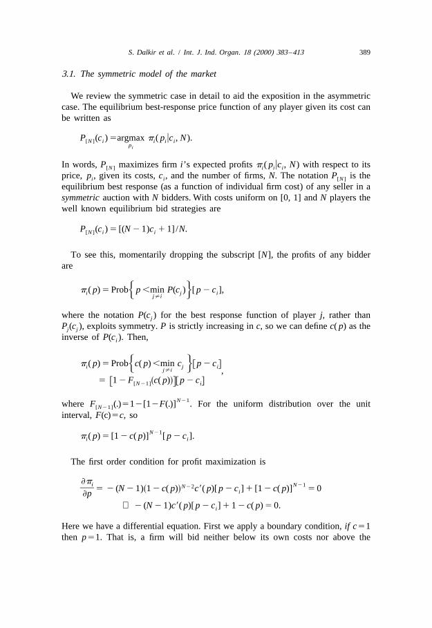
In Fig. 1, we illustrate the cases of N53 and N52, to provide some additionalinsight. Along the cost axis, one quarter is the expected value of the lowest cost inthree cost draws (triopoly). Since the bid is linear in costs, the expected lowestcost (the first order statistic), one quarter, maps directly to the expected triopolyprice, one half. One third is the duopoly expected lowest cost draw, and two thirds

Fig. 1. Equilibrium price functions in symmetric duopoly and symmetric triopoly with uniform costs.

19 This could be stated as a proof by (1) positing that the solution is linear, (2) solving the differentialequation for the above values, and (3) verifying that the first order conditions solve to zero for alladmissible c for these values. We show below that the solution is nonlinear in the asymmetric case.i


is the corresponding expected value of the winning duopoly price. If one were tolook at the price increase from moving from three to two firms in a 1/N symmetricmodel, one would overstate the expected price as two thirds, an increase of onesixth. This process implicitly assumes that the expected minimum cost increasesfrom one quarter to one third, whereas a merger should not be assumed to throwaway technologies leading to higher expected production costs. One might insteadconsider the effects of using the duopoly best responses with the three draw orderstatistic, projecting a postmerger price of five-eighths, an increase of one eighth.Although this does not ‘‘throw away’’ a technology, this too, vastly overstates thetrue price effect of a merger as firms ‘‘act as if’’ this technology were disposed of.To analyze the impact of the merger correctly, we next consider the asymmetricauction model.

3.2. The asymmetric model

In Appendix A we prove that an equilibrium within strictly increasing and20differentiable strategies both exists and is unique. The intuition underlying

existence, the nature of the equilibrium, and hence the nature of the simulation,can be illustrated by looking at the simple case of N53 cost draws, with M52bidders. We first need notation, for the ith firm, we define its number of cost drawsas k . For our example, suppose that draws are distributed with k 51 and k 52.i 1 2

Then, defining c as the ith bidder’s lowest cost draw (the technology it would usei

to fill an order),

(1)c | F (.) ; F(.) and1 1(1) 2c | F (.) ; 1 2 1 2 F(.)f g2 2

where the (superscript) on F denotes the first order statistic (expected lowest cost)for the cumulative distribution of firm i’s costs. The probability density function ofc when F(.) is the uniform distribution over the unit interval is given by2

f(c)5222c. Now the expected profit of bidder 2 is

p ( p ) 5 Prob p , P (c ) p 2 c 5 Prob c ( p ) , c p 2 cf g f gh j h j2 2 2 1 1 2 2 1 2 1 2 2

5 1 2 F c ( p ) p 2 c 5 1 2 c ( p ) p 2 c .f g f gf s dg f g1 2 2 2 1 2 2 2

Unlike in the symmetric case, it is important to use firm subscripts on the bestresponse functions, e.g., P (c ) and its inverse applied to firm 2’s price, c ( p ).1 1 1 2

20 With discontinuous payoffs, a Nash equilibrium in pure strategies need not exist (Dasgupta andMaskin, 1986). To see the discontinuity suppose that, of two bidders, bidder 1 sets price p , where1

p .c . Then bidder 2 gets profits equal to ( p 2c ) if p ,p . Profits increase by increasing p toward1 2 2 2 2 1 2

p from below. But, at p 5p its profits are not equal to ( p 2c ); there is a discontinuity in payoffs.1 2 1 1 2


The final step above simplifies using F(c)5c, the uniform distribution over theunit interval, or U [0, 1].

The expected profit of bidder 1 is

p ( p ) 5 Prob p , P (c ) p 2 c 5 Prob c ( p ) , c p 2 cf g f gh j h j1 1 1 2 2 1 1 2 1 2 1 1(1) 25 1 2 F c ( p ) p 2 c 5 1 2 c ( p ) p 2 c ,f gf g f gs d f g2 2 1 1 1 2 1 1 1

(1)where F is the two draw cumulative distribution function defined above with2

F;U [0, 1].The first order necessary conditions simplify to

9c ( p) 5 (1 2 c ( p)) /( p 2 c ( p))1 1 2

9c ( p) 5 (1 2 c ( p)) /2( p 2 c ( p))2 2 1

with boundary conditions c (a)5c (a)50 for some a[[0, 1) and c (1)5c (1)51 2 1 2

1.Assuming differentiability and exploiting the property that c ,P (c ),1 for alli i i

c ,1, we obtain price functions that are monotonically increasing.i

The boundary conditions imply that for the best response functions and somepoint a, P (0)5P (0)5a (the common vertical intercept), and that P (1)5P (1)51 2 1 2

1 in the upper right corner of the unit square (as in Fig. 2 below). The secondboundary condition implies that if c51 then p51. That is, a firm will bid neitherbelow its own costs nor above the maximal willingness to pay of the buyer. The

Fig. 2. Equilibrium price functions in asymmetric duopoly.


first boundary condition is also intuitive. Suppose that P (0),P (0). Then if firm ii j

has costs c 50, it could raise its price slightly while maintaining certainty of beingi

the winner. Hence P (0),P (0) cannot be a best response price for i, andi j

P (0)5P (0);a must be a boundary condition. Knowing the conditions for an1 2

equilibrium, if one exists, we state our main theorem informally:

Theorem 1: The above problem has an equilibrium and the equilibrium is unique.21A formal statement of the theorem and its proof are in Appendix A.

Given that a unique solution exists, numerical solution techniques can be usedto calculate the expected winning price for any number of bidders with differentnumbers of cost draws. There is known to be a solution to this system of equationsfor some a, so one need only search across solutions satisfying ( p, c)5(a, 0) tofind the unique one which also satisfies ( p, c)5(1, 1). The simulations wereproduced using a fourth-order Runge–Kutta method (Ixaru, 1984; Ascher et al.,1995), and graphical solutions were obtained via functional programming usingMathematica. For details, see Appendix B.

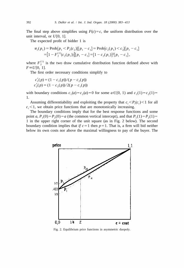
In Fig. 2, we illustrate the best response functions for the case outlined above:two of three firms (each with a single cost draw) merge and the merged firm (firm2) has two cost draws. This is superimposed on the illustration of the symmetricsingle cost draw duopoly and triopoly results. Along the vertical axis, the interceptis a50.421875. Along the cost axis, one quarter is the expected value of thelowest cost draw given three draws from the cost distribution. Unlike thesymmetric case there is no graphical depiction of the expected value of thewinning bid for two reasons: the best response functions are neither linear norcoincident.

Following our example, the expected triopoly price premerger is, as noted¯above, P 50.5. In a duopoly in which firm 2 is the merged firm with two cost[3]

¯draws and firm 1 has one cost draw, the expected duopoly price is P 5merger220.573. These are prices based on the normalization of c[[0, 1]; our calibration to

more ‘‘realistic’’ cost distributions illustrates more modest price effects of merger.

21 Lebrun (1996) provides a fairly general proof of existence in related auctions, and our auction maybe a special case of those that he analyzes. Our proof, albeit a special case, is far more compact.Marshall et al. (1994) recognize the equilibrium existence difficulties and by simulation suggest that anequilibrium both exists and is unique, but do not prove this. They numerically calculate best responsefunctions, stating that ‘‘within numerical accuracy of . . . there is one and only one . . . ’’ solution tothese first order conditions and boundaries.

22 Dalkir (1995) shows that the expected price can be written in terms of the inverse equilibriumprice functions. This expression is numerically integrated across the price range to estimate theexpected price.


Having characterized the solution for an example, we turn to some efficiencyresults.

3.3. Contrasting asymmetric and symmetric auction efficiency

A first-price auction mechanism with symmetric independent private valuesexhibits the revenue equivalence property. It generates the same expected revenueand allocation as a second-price auction mechanism, the highest-revenue direct-revelation auction for the independent private-values model. The bidder with the

23highest valuation (lowest cost) receives the good (contract). Revenue equivalencedoes not hold for asymmetric auctions (Maskin and Riley, 1996). Simply put, withsymmetric auctions all first price auction response functions are identical so thatthe firm with the lowest cost draw bids the lowest price. But, in the asymmetricauction, the first price auction firms’ reaction functions are not coincident. Thegood might not go to the bidder with the lowest cost in the first price auction(whereas it would go to the lowest cost bidder in the second price auction).

This implies a cost inefficiency may arise in the asymmetric first price auction.Using Fig. 2 above, if c 50.25 and Z.c .0.25, firm 1, despite higher costs,2 1

wins the auction. The first impression is that mergers lower efficiency in auctionmarkets. But this is solely because we suppose that the merger creates asymmetry.One might consider an initially asymmetric auction in which a merger creates asymmetric auction and the potential for cost-inefficient bid winning is eradicatedby the merger.

3.4. An asymmetric auction with a merger to symmetry

Since we have characterized the asymmetric auction, we look at the solution to asymmetric auction created by the merger of asymmetric firms. In our context, thisinvolves a symmetric auction with each firm having k>2 cost draws.

Suppose that post merger R>3 firms each have k cost draws: Rk5N, where Nis the total number of cost draws. The best response functions for a game with Rfirms each with k cost draws are identical to the best response functions for thegame with N2k11 firms, each with a single cost draw. (A proof appears inAppendix C.) The intuition for this result is straightforward. In the former gameeach bidder faces R21 rivals with (R21)k cost draws. The first order statistic on(R21)k cost draws determines the expected lowest cost held by a rival. In thelatter game each bidder faces N2k rivals each with a single cost draw. Theexpected lowest cost of a rival comes from the first order statistic from N2k costdraws. Then note that (R21)k5N2k. The rest of the intuition is immediate.Suppose that the best response rule followed by one firm’s rivals in the formergame is identical to that in the latter game. Then clearly the first order condition

23 See, for example, McAfee and McMillan (1987).


for this firm in the former game will be equal to that in the latter game (samemarginal probability of losing as price increases) so it will select the same bestresponse rule as well. From here it is simple to obtain the equilibrium expectedprice, it being the mapping of the first order statistic from N cost draws into thebest response function for the N2k11 single cost draw best response function.

To illustrate briefly, consider a triopoly with two firms each with a single costdraw and one firm with two draws. Merging the first two firms leads to asymmetric duopoly; each firm has two draws. For the uniform c[[0, 1] theasymmetric premerger price is 0.430, and post merger it is 0.467.

We turn now to calibrated models simulating potential biases in merger analysis.

4. Application to merger analysis

There are three issues we wish to address: (1) the profitability of merger, (2) thecalibration of the model and ‘‘realistic’’ price increases from mergers and (3) thesensitivity of the model to our distributional assumptions. We deal with these inorder.

4.1. Is merger profitable?

One question is whether the mergers we model would be profitable to undertake.For policy modeling of mergers one should not use a model which predictsmergers which would not be privately chosen as optimal by the firms involved (cf.,Salant et al., 1983).

Modeling the merger incentive prior to the cost draw, the answer to thisquestion is ‘‘Yes,’’ as all of our simulations demonstrated. While proof wouldrequire several steps, the logic can be expressed simply by looking at one case.Firm i supposes the following. ‘‘If I am the lowest cost firm I will win the auctionat a profit, and if I am not I will earn zero’’ (which is correct in the symmetricpremerger case). Now, suppose that i merges with some other firm (which changesthe possession of the cost draws but not their distribution). The expected value ofthe merged entity would be exactly double the expected value of the unmergedentity if nothing changes (i’s best response or its rivals’). But, if it merges, itrealizes that with some positive probability it has eliminated the second lowestcost firm, leading to a higher best response price as a function of the lower of itstwo cost draws. By definition of a best response, firm expected profitability of themerged entity must hence exceed the profitability of the sum of the two entities ifthere were no merger. Hence i’s (with a partner) expected price rises. This in turnmeans that the M22 firms with a single cost draw each will find it profitable toraise their best responses above the M firm symmetric best responses. This onlymakes it more profitable for firm i (and its partner). Next, suppose that for somerivals’ (symmetric / identical) best response rule the merged entity were to have


lower profits than the sum of the premerger profits of the two entities. Then themerged entity could select instead to bid the premerger best response rule for itslowest cost draw and its expected profits would be greater if its rivals had higherbest response rules, and no lower if they had their initial best response rules. If thiswere to lead to higher expected profits then this must dominate a best responseprice which exceeds this, a contradiction. The best response would then be theinitial best response (or lower).

We now only need to eliminate this counterfactual, that prices would instead belower. Suppose the ith firm were to bid its initial best response rule. Its profitswould be lower only if its rivals were to bid lower prices due to the merger. Forthe rivals to bid lower prices their expectations must be that the merger would leadto a lower price best response rule for the lower cost draw of the two draws for themerged firm i. Firm i would never have an incentive to bid a lower price unless itsrivals independently had an incentive to do so, and in our context firm i couldnever ‘‘credibly commit’’ to do so. Hence it is clear that mergers are profitable.

In contrast, Marshall et al. (1994) find that while coalitions are sustainable andprofitable for small M, they are not sustainable for large M. With M5101, and acoalition of 100 equally sharing coalition profits, they demonstrate that the 101stfirm would not wish to join the coalition. With a coalition of 101 firms, one firmcould leave the coalition and earn greater profits. In their coalitions, all firmsequally share in the profits. For merger analysis, however, an acquiring firm canchoose how much profits to offer to a potential merger partner, which can in turndecide whether to accept the merger proposal. For a merger one can calculate fromtheir table that for one firm with 100 cost draws and one firm with only one costdraw a Pareto-preferable merger exists. Following a merger logic, the 100 drawsare not separate firms in a coalition capable of withdrawing and free-riding.Bribing a firm to join, i.e., paying a purchase price in excess of opportunity costs,leads to no free-rider problem as that final ‘‘plant’’ or ‘‘draw’’ becomes part of a

24single legal entity.

4.2. Calibration and simulation of merger price effects

Calibration of such a model depends upon the available data. When possible,econometric analysis of the market can yield estimates of marginal costs, demand

24 We have not dealt with the ‘‘hold out’’ problem. That is, we do not prove that there exists a seriesof mergers that would lead 101 firms to merge sequentially, only that at the margin one merger isprofitable. Waehrer (1997), for example, demonstrates that one would prefer to free ride others’ mergersin such models.


25elasticities and the like. Here, we proceed by calibrating the model via market26shares and the coefficient of spread (spread/mean ratio).

There are two elements to calibrate: (1) market shares prior to merger and (2)the range of the density function of costs, [m 2D, m 1D] or [m(12d), m(11d)]where d;D /m is the coefficient of spread. For an example, start with a symmetricmarket. Then, normalizing cost draws from the range c[[0, 1] to c[[100(12d),100(11d)], we can calibrate the model to the coefficient of spread for a singlebidder. In actual merger cases reasonable estimates of d can be elicited from thetechnical staff (‘‘engineers’’) or from the administrators who are informed about

¯costs. The premerger expected winner’s price is P5100[4d /(N11)112d] and¯the premerger expected winner’s cost is c5100[2d /(N11)112d].

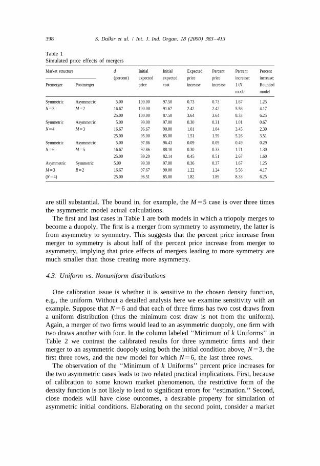
Suppose that d is between 5% and 25%, in the real world d is unlikely to exceed25%. Then one can derive the normalized premerger price and cost for a given Nto simulate the effects of merger. We illustrate with mergers of symmetric firms, inmarkets with N53, N54, and N56, in Table 1 below. Similarly, it is possible tocalibrate the price increase from asymmetric firms merging to become symmetric.To demonstrate, consider the merger of three asymmetric firms (M53) into twosymmetric firms, as in the above section. The results are shown in Table 1.

Despite the small numbers of firms, the simulations suggest that the unilateraleffects from a merger (using the true model) are modest at worst. For example, theGuidelines often focus on a five percent price increase as ‘‘significant.’’ None ofthe simulated price increases is greater than five percent. This may be a convincingbasis for approval of a merger, especially if moderate efficiency gains are likely(cf., Willig, 1997).

From Table 1, the percent increase predicted by the ‘‘naive’’ 1 /N formula isslightly higher than M times (resp. N times) the true increase for an asymmetric(resp. symmetric) merger. This provides a rough rule of thumb for inferring thetrue price increase from the 1/N formula. We also mentioned that we could boundprice effects by looking at price increases from mergers using the 1/N and1/(N21) best response functions, but using the limit statistic for N cost draws.This is used in the final column in Table 1. This roughly eliminates half of the biasfrom using the 1/N rule, but with such a huge bias from the 1/N rule, the biases

25 In individual markets these bids are few and contracts are of long duration. Hence standard timeseries cannot be of much use. To use cross sections to calibrate one must assume that all of the marketshave the same technologies and demands. Furthermore, if one has the cross section information tocalibrate this model and one is willing to assume that each market has the same technological anddemand conditions, then one should have sufficient data to predict the effects of market structure onprice directly through regression simulation without imposing this theoretical structure.

26 Alternatively, we could have chosen to calibrate using the coefficient of variation, s /m, which, for]Œthe uniform distribution, is equal to d / 3. Calibration could also start from premerger Price Cost

Margins or other data.


Table 1Simulated price effects of mergers

Market structure d Initial Initial Expected Percent Percent Percent

(percent) expected expected price price increase: increase:

Premerger Postmerger price cost increase increase 1 /N Bounded

model model

Symmetric Asymmetric 5.00 100.00 97.50 0.73 0.73 1.67 1.25

N53 M52 16.67 100.00 91.67 2.42 2.42 5.56 4.17

25.00 100.00 87.50 3.64 3.64 8.33 6.25


N54 M53 16.67 96.67 90.00 1.01 1.04 3.45 2.30

25.00 95.00 85.00 1.51 1.59 5.26 3.51


N56 M55 16.67 92.86 88.10 0.30 0.33 1.71 1.30

25.00 89.29 82.14 0.45 0.51 2.67 1.60

Asymmetric Symmetric 5.00 99.30 97.00 0.36 0.37 1.67 1.25

M53 R52 16.67 97.67 90.00 1.22 1.24 5.56 4.17

(N54) 25.00 96.51 85.00 1.82 1.89 8.33 6.25

are still substantial. The bound in, for example, the M55 case is over three timesthe asymmetric model actual calculations.

The first and last cases in Table 1 are both models in which a triopoly merges tobecome a duopoly. The first is a merger from symmetry to asymmetry, the latter isfrom asymmetry to symmetry. This suggests that the percent price increase frommerger to symmetry is about half of the percent price increase from merger toasymmetry, implying that price effects of mergers leading to more symmetry aremuch smaller than those creating more asymmetry.

4.3. Uniform vs. Nonuniform distributions

One calibration issue is whether it is sensitive to the chosen density function,e.g., the uniform. Without a detailed analysis here we examine sensitivity with anexample. Suppose that N56 and that each of three firms has two cost draws froma uniform distribution (thus the minimum cost draw is not from the uniform).Again, a merger of two firms would lead to an asymmetric duopoly, one firm withtwo draws another with four. In the column labeled ‘‘Minimum of k Uniforms’’ inTable 2 we contrast the calibrated results for three symmetric firms and theirmerger to an asymmetric duopoly using both the initial condition above, N53, thefirst three rows, and the new model for which N56, the last three rows.

The observation of the ‘‘Minimum of k Uniforms’’ percent price increases forthe two asymmetric cases leads to two related practical implications. First, becauseof calibration to some known market phenomenon, the restrictive form of thedensity function is not likely to lead to significant errors for ‘‘estimation.’’ Second,close models will have close outcomes, a desirable property for simulation ofasymmetric initial conditions. Elaborating on the second point, consider a market


Table 2Calibrated price increases: uniform cost distribution vs. nonuniform cost distributions

Market structure Percent Percent Percent pricespread d coefficient increase

Premerger Postmerger of the of variationuniform Minimum Extreme

of k valueuniforms

Symmetric Asymmetric 5.00 2.89 0.73 0.54Triopoly Duopoly 16.67 9.62 2.42 1.83k51 k 52 25.00 14.43 3.64 2.76merger

k 51nonmerger

Symmetric Asymmetric 5.00 2.40 0.66 0.54Triopoly Duopoly 16.67 8.32 2.31 1.92k52 k 54 25.00 12.86 3.58 3.01merger

k 52nonmerger

with three firms with asymmetric market shares. One could simulate shares usingthe uniform distribution on [0, 1] by varying cost draws, k 1k 1k 5N. If one1 2 3

had a similar market in terms of shares, one might require a significantly differentN (e.g., 9 /32 is very close to 1 /4) to simulate the initial shares. The stability of thecalibrated results (not those on [0, 1]) with respect to N implies that for ouralgorithm similar starting shares yield similar results on merger consequences.

Our distributional assumption is likely closer to being an upper bound on theextent of the merger price increase, over different types of distributions. Forfurther sensitivity analysis with respect to the type of the distribution, we

27compared our results with those from an extreme value distribution, as in28Tschantz et al. (1997). In the above section we used the spread parameter d to

calibrate the price increases under the uniform; we do the same in Table 2. Inorder to hold the coefficient of variation constant across the two distributions, weneed to calibrate the extreme value distribution to the coefficient of variationimplied by d. Each value of the spread parameter d implies a different value forthe standard deviation s, and hence a different coefficient of variation, s /m. Thecoefficient of variation (s /m) of a uniform distribution can be expressed as a

]Œsimple function of its spread parameter d, as s /m 5d / 3.On the first set of rows of Table 2 (premerger k51), the expected price

increases under ‘‘the minimum of k uniforms’’ are equivalent to those on the firstrow of Table 1 under the true model with uniform costs (minimum of one uniformrandom variable is equivalent to the uniform random variable itself). On the samerow, the price increases under ‘‘extreme value’’ are coming from an extreme valuedistribution with the same coefficient of variation s /m corresponding to each d.

27 The extreme value density is f(x)5exp[2(x2a) /b] exph2exp[2(x2a) /b]j /b for 2`,x,1`2 2with mean5a1(0.57721)b and variance5b p /6.

28 We would like to thank Luke Froeb for assistance in this calibration.


On the second set of rows of Table 2 (premerger k52), the expected priceincreases under ‘‘the minimum of k uniforms’’ are from a merger between two outof three symmetric firms, each with two cost draws; each cost draw is distributeduniformly with m 5100 and spread parameter d. Now the minimum of twouniform costs does not have a uniform distribution, and its mean and variance aredifferent than those of the underlying uniform distribution. The coefficient ofvariation (s*/m*) of the minimum cost is related to the spread parameter d of each

]Œof the two uniform costs, as s*/m*52dm /(3 2m*). The expected price increasesunder ‘‘extreme value’’ are coming from an extreme value distribution with acoefficient of variation s*/m*.

We display the percent price increases for the two types of distributions in Table2. For the asymmetric merger case with uniform costs (premerger k51), thepercent price effect from the extreme value distribution is approximately three-quarters of our prediction. For the nonuniform case (premerger k52), it isapproximately 83% of ours.

Some variation is shown to alternative choices of the distribution used in thecalibration, but the results changed little. And, for whatever variation does existacross distributions, it appears that the uniform, with its ‘‘fat tails’’ tends torepresent a ‘‘worst case’’ scenario in terms of merger price effects.

5. Compensating merger efficiencies

Welfare effects in auction markets are usually small because of the perfectlyinelastic demand; the only welfare loss occurs in a first price auction when the‘‘wrong’’ firm wins the auction, not because the buyers turn away from theproduct. Enforcement agencies may ask how much the expected cost of themerging parties would have to go down (i.e. the size of the ‘‘merger-specificefficiencies’’) in order to counteract the price effect of the merger.

To get an idea about the magnitude of the merger-specific cost savings thatwould exactly offset the merger’s price effect, we first calibrated the merger firm’scost distribution such that the postmerger price is the same as the premerger pricein the absence of efficiencies. Technically, we redefined the merger firm’s cost

(1) 21edistribution as F (.)512[12F(.)] where F(c)5c is the uniform distribution,2

while keeping the nonmerger firm’s distribution as the uniform. This has the effectof lowering the mean and the variance of the distribution, while holding its

29support. We increased ´ until the postmerger equilibrium price (from new bestresponse price functions for both firms based on the new set of distributions) was

29 (1:z) zThe distribution F (.)512[12F(.)] has the nice interpretation of being the distribution of theminimum of z independent draws from distribution F, where z is an integer. With merger-specificefficiencies, we can model this as if the firm had an additional (fractional) draw from the distribution.

(1:z) (1:z)The mean of F when F is the uniform over [0, 1] is m 51/(z11). Accordingly, if prior tomerger we have z51 and post merger we treat this as z52, we can model efficiencies by simply usingthe fractional form, z521´ which has a lower mean cost.


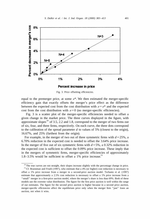
Fig. 3. Price offsetting efficiencies.

equal to the premerger price, at some ´*. We then estimated the merger-specificefficiency gain that exactly offsets the merger’s price effect as the differencebetween the expected cost from the cost distribution with ´5´* and the expectedcost from the cost distribution with ´50 (no merger-specific efficiencies).

Fig. 3 is a scatter plot of the merger-specific efficiencies needed to offset agiven change in the market price. The three curves displayed in the figure, with

30approximate slopes of 3.5, 2.2 and 1.8, correspond to the merger of two firms outof six, four, and three firms, respectively. On each curve, the three dots correspondto the calibration of the spread parameter d to values of 5% (closest to the origin),16.67%, and 25% (farthest from the origin).

For example, in the merger of two out of three symmetric firms with d525%, a6.70% reduction in the expected cost is needed to offset the 3.64% price increase.In the merger of five out of six symmetric firms with d55%, a 0.32% reduction inthe expected cost is sufficient to offset the 0.09% price increase. These imply thatin the mergers of symmetric firms, merger-specific efficiencies of approximately

311.8–3.5% would be sufficient to offset a 1% price increase.

30 The true curves are not straight, their slopes increase slightly with the percentage change in price.31 Cf. Brannman and Froeb (1997), who estimate that a 4% (or higher) cost reduction is necessary to

offset a 1% price increase from a merger in a second-price auction model. Tschantz et al. (1997)estimate that approximately a 2.5% cost reduction is necessary to offset a 1% price increase from a‘‘small’’ merger in a first-price auction model, where the merger’s share is less than 69%. Both of thesemodels use the extreme value distribution. The figure for the first price auction is well within the rangeof our estimates. The figure for the second price auction is higher because in a second price auction,merger-specific efficiencies affect the equilibrium price only when the merger firm ‘‘just’’ loses anauction, not when it wins.


Williamson (1968) showed that welfare gains from merger efficiencies canoffset the losses due to a higher price. We assume that a merger’s expected cost islower than either of the merging parties’ premerger expected cost; simultaneouslythere is an increase in the expected price due to the change in the number of firms.Consequently, the merger has to aim for additional efficiencies if it wants tobalance off the price effect. Our results confirm the basic Williamsonian insight ina specific equilibrium oligopoly equilibrium model.

6. Extensions

Market-specific issues may arise in a particular application. To explore these,we return to the application to hospital mergers. Hospitals may provide a vector ofservices, e.g., services A and B (cardiac and obstetrics). In the context of the abovemodel this leads to another implication for mergers (cf., Dalkir, 1995 for a formaltreatment). Suppose that for a PPO, a hospital must bid for the vector of hospitalservices (which is what we observe in practice). Each hospital receives a cost draw

32for each service, A and B. A merged hospital selects the lower cost of twosignals for procedure A and for procedure B. It is then simple to demonstrate thatfor PPO bids, a merged hospital has a lower expected cost for the combined sale ofA and B than the expected costs of the two nonmerged entities. Hence, hospitalmergers are likely to yield cost savings since only one bid winner provides thecomplete vector of services to the PPO.

In an application Dalkir (1995) demonstrates that for i.i.d. cost draws, initialcalibrations, and some market structures, this cost advantage from the combinationof services may be substantial. Merger price increases from such a model will beless than in the corresponding single service model and the efficiency gains mayeven outweigh price effects. This could not be demonstrated using either the naiveor bounded models. In particular for such market structures the importance ofusing the asymmetric auction model for merger simulation establishes a presump-tion for a merger that could not be established by use of an analytically simplersymmetric auction model.

7. Concluding remarks

Despite the new trend towards use of unilateral effects models for mergeranalysis, still most merger cases, even ones for which the presumption is one of

32 For the effects noted, one must assume that the cost draws are not linearly dependent, e.g., the costof A is not a times the cost of B for both hospitals.


unilateral action, are decided using ‘‘structural indices.’’ That is, concentration(HHI) levels and changes play an important role, whereas modeling does not playa big role in most cases. As this is shifting to more use of explicit unilateral effectsmodeling, our modeling approach may be useful for calibration in more caseswhen they involve auction sales. As we demonstrate, the analytically tractable 1 /Nmodels would lead to misleadingly huge calibrated unilateral effects of mergers inauction markets. Our method of solution for the asymmetries implied by mergersshow that these are important to understand when predicting price effects ofmergers and that, when unilateral effects, rather than collusion, are the concerns ofthe antitrust agencies, that price effects in auction mergers appear to be quitemodest relative to what one would expect from application of these simplermodels.

Having a model is also useful for other considerations. For example, theprospects for entry post merger will change with a merger. Indeed, we can see thisby looking at the first two cases in Table 1 (using d516.67 for simplicity). If thereare N53 symmetric firms, the initial expected price is 100, entry of one more(identical) firm would lead to four firms and a price of 96.67. If there were amerger from N53 to M52, and no efficiency effects, then price would be 102.42,and entry would lead to the case labeled M53 below, with expected price of97.68, entry is more likely post merger. With predictions like these and knowledgeof industry characteristics, profitability, potential entrants and the like, antitrustagencies can assess with greater accuracy the likelihood of entry in the absence ofefficiency gains from the merger.

This type of ‘‘entry’’ information is particularly important to know for auctionmarkets in which bid preparation is costly. In some cases the cost of bidpreparation substantial. (E.g., it may involve costly exploration or significant Rand D simply to respond to a request for a proposal.) In such cases there may bemore producers of the product than there will be bidders in a two stage game inwhich firms must first ‘‘prepare the bid’’ and then there is ‘‘bidding by those firmswhich prepared a bid.’’ But, it may be that there is very little change inprofitability of entry (preparing the bid) before an additional firm would enter intothe auction. These and other factors can be used to increase the power of themodel in actual application.

Acknowledgements

We would like to acknowledge input from Kenneth C. Baseman, DavidEisenstadt, and Frederick R. Warren-Boulton of Micra, Luke M. Froeb ofVanderbilt University, Robert J. Reynolds of Competition Economics, RamseyShehadeh of Cornell University, and two anonymous referees. The viewsexpressed do not necessarily reflect those of the employers.


Appendix A

33Proof of the main theorem

The asymmetric first-order equilibrium conditions derived in the text assume34that the equilibrium strategies are strictly increasing, hence invertible. Addition-

ally, the proof rests upon the following two arguments: (i) that the set of possiblesolutions for the asymmetric first-order conditions is connected, and (ii) that thestrategies of the two asymmetric players do not cross in the interior of theprice3cost space.

The equilibrium requires solving the differential-equation first order conditionswith two boundary conditions, a common initial point, a, where c50 and acommon terminal point of value 1 where c51. Although one is assured of asolution to a system like our first order conditions with one boundary condition(cf., Theorem 11.1 in Ross, 1964), there is no general proof for the existence, oruniqueness, for the solution of two differential equations with two boundaryconditions. Using standard differential equations notation, we provide a proofherein. In this notation, y(t) is our inverse best response function (c( p) in the text),and t is the initial condition (a in the text).0

With this notation, our first order conditions are the inverse price functions

9 9y 5 (1 2 y ) /(t 2 y ), y 5 (1 2 y ) /2(t 2 y )1 1 2 2 2 1

which satisfy for an initial value t [(0, 1], the initial condition and t51, the0

terminal condition. Denote, using vector notation, y;( y , y ), f(t, y);( f (t, y),1 2 1

f (t, y)), where f (t, y);(12y ) /(t2y ) and f (t, y);(12y ) /2(t2y ). We then2 1 1 2 2 2 1

have the Boundary Value Problem

y9 5 f(t, y)y(t ) 5 (0, 0)(BVP) 05y(1) 5 (1, 1)

Then ask whether there is any t [(0, 1] such that when t 5t , the solution of the* 0 *

Initial Value Problem

y9 5 f(t, y)(IVP) Hy(t ) 5 (0, 0)0

33 We thank Kevin Hockett of The George Washington University, Jerrold E. Marsden of Caltech andLars Wahlbin of Cornell University for their comments on this proof.

34 We can justify a priori that the equilibrium strategies must be nondecreasing, but strictmonotonicity is verified by the actual shape of the numerically-estimated equilibrium strategies.


t t t0 0 0is also a solution of (BVP). Let y 5 ( y , y ) be the notation for the pair of1 2

functions that solve (IVP). Formally our goal is to prove:

tTheorem. There is a unique t [(0, 1] such that the solution y of (IVP)**t tsatisfying y (t )5(0,0) is also a solution of (BVP), satisfying y (1)5(1, 1).* **

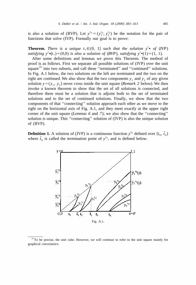
After some definitions and lemmas we prove this Theorem. The method ofproof is as follows. First we separate all possible solutions of (IVP) over the unit

35square into two subsets, and call these ‘‘terminated’’ and ‘‘continued’’ solutions.In Fig. A.1 below, the two solutions on the left are terminated and the two on theright are continued. We also show that the two components y and y of any given1 2

solution y5( y , y ) never cross inside the unit square (Remark 2 below). We then1 2

invoke a known theorem to show that the set of all solutions is connected, andtherefore there must be a solution that is adjoint both to the set of terminatedsolutions and to the set of continued solutions. Finally, we show that the twocomponents of that ‘‘connecting’’ solution approach each other as we move to theright on the horizontal axis of Fig. A.1, and they meet exactly at the upper rightcorner of the unit square (Lemmas 6 and 7 ); we also show that the ‘‘connecting’’solution is unique. This ‘‘connecting’’ solution of (IVP) is also the unique solutionof (BVP).

t0 ˜Definition 1. A solution of (IVP) is a continuous function y defined over [t , t )0 0t0˜where t is called the termination point of y , and is defined below.0

Fig. A.1.

35 To be precise, the unit cube. However, we will continue to refer to the unit square mainly forgraphical convenience.


t0Remark 1. (IVP) has a unique solution y for any t [(0, 1] on any interval over0

which f satisfies the Lipschitz condition, by ‘‘The Basic Existence Theorem’’ forODEs (Ross, 1964). This theorem holds for (IVP) because f is differentiable, anddifferentiability implies that the Lipschitz condition is satisfied.

t0Definition 2. The termination point, or limit fixed point, if any, of y such thatt0 ˜ ˜y (t) → t as t → t .1 0 0

t t0 0˜Definition 3. If y (t) has a termination point t ,1 then y is called a terminated1 0t0˜ ˜solution defined over [t , t ). If y (t) does not have a termination point t ,1 then0 0 1 0

t t0 0y is called a continued solution defined over [t , 1]. If y is a continued solution,0˜then we let t 51 for notational convenience.0

t0Definition 4. An extension of a terminated solution y ist t0 0 ˜y (t) 5 y (t) over [t , t ),0 0

t t0 0 ˜˜y (t) 5 y at t ,0

t t t t0 0 0 0˜˜ ˆ 9where y is defined as lim y (t). We also define (y (t ) as lim ( y )9(t),˜ ˜t→ t 0 t→t 0

which needs not be finite.

t0Lemma 1. There exists some separation point s[(0, 1] such that for t ,s,y is a0t0terminated solution of (IVP) and for t .s, y is a continued solution of (IVP).0

Proof. It is easy to show that the second derivatives can be written as

99 9 9 99 9 9y 5 y ( y 2 2) /(t 2 y ) and y 5 y ( y 2 3/2) /(t 2 y ).1 1 2 2 2 2 1 1

One can then write

99 9 99 9y . 0⇔y . 2 , y . 0⇔y . 3/2 ,h j h j1 2 2 1

9 9 9 9since y .0 and y .0. Given those, and y 5(12y ) /(t2y ) and y 5(12y ) /1 2 1 1 2 2 2t t1 20 0

] ]2(t2y ), we claim that for all t , , y is terminated and for all t . , y is1 0 04 3

continued. Therefore we claim that both types of solutions actually exist.t1 0

]For all t , , y is terminated because not only are y and y ‘‘steep’’ (their0 1 24

slopes exceed 4 and 2 respectively at t ), but also convex ( y is convex because0 1

the slope of y is greater than 2, and y is convex because the slope of y is greater2 2 1

than 3/2), therefore they become even steeper (reinforcing each other’s convexity)˜for greater values of t; y intercepts the diagonal at some t ,1. Similarly, for all1 0

t2 0]t . , y is continued because not only are y and y ‘‘flat’’ (their slopes are0 1 23

smaller than 3/2 and 3/4 respectively at t ), but also concave ( y is concave0 1

because the slope of y is less than 2, and y is concave because the slope of y is2 2 1

less than 3/2), therefore they become even flatter (reinforcing each other’s


concavity) for greater values of t, and remain below the diagonal for all values oft<1. We conclude that both types of solutions exist.

Now suppose that Lemma 1 is not correct, then there must exist initial points t ,1t t t t1 2 3 4t , t , t such that y , y are terminated and y , y are continued (see Fig. A.1),2 3 4

t5and such that one can find t in the open interval (t , t ) with y continued, or t in5 1 2 6t0the open interval (t , t ) with y terminated, or both. This contradicts the3 4

uniqueness of the solution to (IVP) at some point. From Remark 1 above,uniqueness in (IVP) implies that solutions starting from different initial pointscannot cross, but this is exactly what would happen if the set of solutions was notseparated. QED

Definition 5. Let S(I) define the set of all solutions of (IVP) defined over interval1I,(0, 1] and let S be the notation for the set of solutions of (IVP) with initial

points in the interval J,(0, 1]. Then define

S (I) 5 y [ S(I), y is terminatedh jT

S (I) 5 y [ S(I), y is continued .h jC

J J JS and S are defined for y[S similarly.T C

Remark 2. The strategies of the two asymmetric players do not cross in theinterior of the price3cost space, that is, y (t) and y (t) do not cross at any t,11 2

for any solution y(t) of (IVP). Indeed, observe that y .y in some neighborhood1 2

9 9of t because y (t ).y (t ). Then let t .t be the first point at which y and y0 1 0 2 0 1 0 1 2

cross (but are not equal to one, which is what we are trying to prove). To this end,9let y (t )5y (t )5a ,1 for some a .0. Then y (t )5(12a) /(12a)51 and1 1 2 1 1 1

9y (t )5(12a) /2(12a)51/2, i.e., at t , y is steeper than y , a contradiction.2 1 1 1 2

Since y .y at all points to the left of t , y has to be steeper than y at t .1 2 1 2 1 1

˜ ˜ ˜ ˜Remark 3. It follows that y ±y implies y ,y because y <y for all y over [t ,2 1 2 1 2 1 0

t ) ( from Remark 2 ).0

Lemma 2. Let ht j be a sequence in the open interval (0, 1), with limit t . Over ann 0t t t tn 0 n 0interval on which the solutions of (IVP) y , y exist, y → y uniformly as

t →t .n 0

Proof. Follows from the continuous dependence of the solutions with respect tothe initial values as stated and proven by, for example, Pontryagin (Pontryagin,1962, Theorem 15, pp. 179–181).

t t t t t tn 0 n 0 0 0˜ ˜ˆ ˆ ˆ ˆLemma 3. If y → y on [t , t ) then y →y and (y )9→(y )9 on [t , t ].0 0 0 0

ˆ ˆProof. Follows from Lemma 2 and the continuity of y and y 9.


J JLemma 4. S (I) is connected for any I. Moreover, if J is compact then S (I) iscompact.

JProof. Let G be the mapping, G :J→S (I) for arbitrary subintervals I, J of (0, 1]tnsuch that G(t )5y on I. From Lemma 2, G is continuous. Since J is connected,n

J JS (I) is connected. If J is compact, so is S (I). QED

ˆ ˜ ˜Lemma 5. Let S(I) be the set of solutions over I extended from [t , t ) to [t , t ]0 0 0 0ˆby taking limits. Then S(I) is connected.

Proof. Follows from Lemmas 3 and 4.

˜ ˜Lemma 6. There is no solution such that y ,y 51.2 1

˜ ˜Proof. Suppose y[S satisfies y ,y 51. As above, we can write2 1

99 9 9 99 9 9y 5 y ( y 2 2) /(t 2 y ) and y 5 y ( y 2 3/2) /(t 2 y ),1 1 2 2 2 2 1 1

hence

99 9 99 9y . 0⇔y . 2 , y . 0⇔y . 3/2 .h j h j1 2 2 1

Moreover, it can be shown that299 9 99 99 9( y ) y y 1 y ( y 2 1)2 2 1 2 1

]] ]]]]]]999y 5 1 .2 9y t 2 y2 1

9If y ,1 and y →1 as t→1 then y 5(12y ) /2(t2y )→1`. Now we will first2 1 2 2 1

99prove that y .0 as t→1, and then show that there is a contradiction.2

9 9There is some t ,1 at which y is finite. Since y goes from a finite value to1 2 2

infinity, we can find some t at which it is both large and increasing. It follows that2

99 999y .0 at t . Now look at y at t , its first term is clearly positive. Its second term2 2 2 2

9 99 99is positive because y is large, implying y .0. Furthermore, y .0 at t implies2 1 2 2

9 99y .3/2, therefore the third term is also positive at t . We conclude that y is1 2 2

9monotonically increasing not only at t but at all t.t , which implies y .3/2 for2 2 1

9all t.t . This contradicts y ↓0, given y ,1 and y →1 as t→1, from its definition2 1 2 1

9y 5(12y ) /(t2y ). QED1 1 2

˜ ˜ ˜ ˜Lemma 7. If for y[S, y <y 51 then y 5y 51.2 1 2 1

Proof. Consequence of Lemma 6.Now we prove the main Theorem on the existence and uniqueness of

equilibrium.

Proof. Above we showed that a separation point s exists between the initial points


for S (that lie to the left of s) and the initial points for S (that lie to the right ofT C

s). Clearly, s is in the closures of both intervals (0, s) and (s, 1]. From Lemmas 2s sând 3, y is a limit solution for both S and S , and y is a limit solution for bothT C

s sˆ ˆ ˜S and S . Suppose y does not solve (BVP). Specifically, assume y 5d ,1 forT C 1s s ˆ ˜ˆsome d .0, then clearly y does not solve (BVP). If y is in S , let s be itsT

tn˜termination point. Now ask whether there exists a sequence y in (0, 1] that1t t sn nˆ ˜ ˜ ˜ˆcorresponds to the sequence y in S such that (1, y →(s, y ). The answer isC 1 1

s˜ ˜clearly ‘‘No’’ since s5y 5d ,1. Therefore such a sequence does not exist. This1ˆviolates the connectedness of S.

s ˆ ˆ ˜Îf y is not in S then by definition it is in S , with s51. We ask whether thereT Ct tn n˜ ˜˜ îs a sequence (t , y ) in (0, 1]3(0, 1] that corresponds to the sequence (t , y ) inn 1 n

t s tn nˆ ˜ ˜˜ ˜ ˜(0, 1]3S such that (t , y )→(1, y ). The answer is ‘‘No’’, since t 5y andT n 1 1 n 1sy 5d ,1. Therefore such a sequence does not exist. Again, this violates the1

ˆconnectedness of S.s s˜ ˜We conclude that the assumption was wrong and y 51. From Lemma 7, y 51.1 2

s s 36ˆMoreover, at t51, ( y )953/2 and ( y )952, using l’Hopital’s Rule. Therefore1 2s s s s( y )(1)5f(1, y (1)) with y (1)5(1, 1) is bounded, and y (1) is well-defined.

sUniqueness of y , i.e. uniqueness in (BVP), follows from uniqueness in (IVP)(Remark 1 ). Setting t 5s completes the proof of the main Theorem.*

Appendix B

The numerical solution

This appendix contains a Mathematica program to numerically solve andgraphically display any system of two ordinary differential equations g (t) and1

g (t), whose derivatives are represented by functions f (t, g (t), g (t)) and f (t,2 1 1 2 2

g (t), g (t)) respectively. The estimation technique is ‘‘explicit fourth-order1 2

Runge–Kutta.’’ For further details see Ixaru (1984) pp. 133–34 and Ascher et al.(1995) pp. 68–72 and 210–17. We tried uniform step sizes ranging from order of

23 2510 to 10 , the solutions of the boundary value problem identified by using37different step sizes were reasonably close to each other. A fourth-order Runge–

36 9 9 9Taking the derivative of each numerator and denominator separately, y 52y /(12y ) and1 1 2

9 9 9y 52y /2(12y ) gives the result.2 2 137 thA q -order Runge–Kutta method is a numerical solution algorithm which uses the values of the

n nfunctions and their derivatives at point t to evaluate the value of the function at point t 1h (where h isthe step size) by running q consecutive approximations and taking their weighted average at each step.

n nSince the approximation at t 1h depends on the data at t only, Runge–Kutta is a one-step method.For q51, the method is identical to the Euler algorithm (linear extrapolation).


38Kutta method with a uniform step size is consistent of order 4, the maximum39 40order of consistency attainable by Runge–Kutta.

The program logic

1. At an arbitrary initial point the values of the functions and the derivatives aren n n n nknown analytically. Let this point be t , and let g (t )5g and g (t )5g . If there1 1 2 2

is any other function p related to g (t) and g (t) that needs to be evaluated (e.g.1 2n n n np5expected price), let p(t , g , g )5p be its initial value. Defining h as step size1 2

n n n n n n2. Estimate: k 5hf (t , g , g ), l 5hf (t , g , g ), the increments to g and g1 1 1 2 1 2 1 2 1 2

by linear extrapolation, using the derivatives at the initial point.n n n n3. Estimate: k 5hf ((t 1h /3), ( g 1k /3), ( g 1l /3)), l 5hf ((t 1h /3),2 1 1 1 2 1 2 2

n n( g 1k /3), ( g 1l /3)), repeat starting at initial value plus a third of the first1 1 2 1

estimate, at one-third of the step length.n n n n4. Estimate: k 5hf ((t 12h /3), ( g 2k /31k ), ( g 2l /31l )), l 5hf ((t 13 1 1 1 2 2 1 2 3 2

n n2h /3), ( g 2k /31k ), ( g 2l /31l )), again average now first two estimates, at1 1 2 2 1 2

two-thirds of the step length.n n n n5. Estimate: k 5hf ((t 1h), ( g 1k 2k 1k ), ( g 1l 2l 1l )), l 5hf ((t 14 1 1 1 2 3 2 1 2 3 4 2

n nh), ( g 1k 2k 1k ), ( g 1l 2l 1l )), averaging first three estimates, at the end1 1 2 3 2 1 2 3

of the step.m n6. Evaluate the functions g and g at the end of the step (at t 5t 1h) as the1 2

nvalue in the beginning of the step (at t ) plus a weighted average of the first fourm m nstep estimates k , . . . ,k or l , . . . ,l . That is, g 5g (t )5g 1(k 13k 13k 11 4 1 4 1 1 1 1 2 3

m m nk ) /8 and g 5g (t )5g 1(l 13l 13l 1l ) /8.4 2 2 2 1 2 3 4m n m m m7. Evaluate, for further use, p 5p 1p(t , g , g ).1 2

m m m8. Go to the beginning of the algorithm, repeat the steps substituting t , g , g1 1n n nfor t , g , g , n50, 1, 2, . . . , m5n11.1 2

9. Repeat until the maximum number of steps is reached.n n n n10. Save consecutive pairs (t , g ), (t , g ) in lists list , list , later, plot these1 2 1 2

lists.11. Print the last values obtained before stopping, including the final value of p.

If the solutions have gone over the 458-line or they are not ‘‘close enough’’ to the

38 In numerical solution parlance, a numerical solution method is consistent of order p if the localtruncation error (the difference between the true solution and the estimated solution at one step only) is

pat most of order h where h is the step size. In contrast, a method is convergent of order p if the globalperror (accumulated local errors) is at most of order h . For one-step methods, including Runge–Kutta,

a method is consistent if and only if it is convergent (Ascher et al., 1995, p. 71). In general, the globalp21 perror is at most of order h if the local order is at most of order h . This conveniently provides an

upper bound on the size of the truncation error in our estimates.39 That is, a Runge–Kutta algorithm that uses q.4 separate approximations at each step is consistent

of order 4 only (Ixaru, 1984, p. 135).40 For estimation algorithms alternative to ours, see Riley and Li (1997) and Bajari (1996).


0boundary values g (1)5g (1)51 then change the value of the starting point t1 20 0 0(but keep the starting values of g , g , p because they must hold at any starting1 2

point) by moving it to the right or to the left on the [0, 1] interval. In our problemthese initial values were all zero.

The program

-

Appendix C

Symmetric multiple draw auctions

In this appendix we show that the symmetric profit function for N draws and Rfirms, each with k5N /R>2 cost draws is identical to the symmetric profitfunction for N2k11 firms, each with a single cost draw.

First we will show that the multiple cost draw leads to an equivalent expectedprofit function to a corresponding single cost draw game. Firm i’s expected profits

˜in the multidraw game as a function of its price p , for any value of its lowest costi

˜draw c , isi


˜˜ ˜ ˜ ˜ ˜ ˜p (p ) 5 Prob p ,min P (c ) [p 2 c ].H Ji i i j j i ij±i

˜ ˜ ˜By symmetry, the function P ;P for all j. Exploiting P being positively sloped inj

˜ ˜c and defining its inverse as c(p )

˜ ˜ ˜ ˜ ˜ ˜ ˜p (p ) 5 Prob c(p ) ,min c [p 2 c ].H Ji i i j i ij±i

˘Denote i’s rivals as 2i, their lowest cost as c with N total cost draws, k by firm2i

i, then the distribution of rivals’ minimum cost is

(1) N2k˘ ˘ ˘F (c ) 5 1 2 F(c )f g2i 2i 2i

so

N2k˜ ˜ ˜ ˜ ˜ ˜p (p ) 5 1 2 F c(p ) [p 2 c ].f s dgi i i i i

where F;U [0, 1], the uniform distribution over [0, 1].We now turn to the game where each player has a single cost draw. Recall in

this game, if there are N9 firms (and hence draws) the first order conditions aregiven by

(1)p ( p) 5 Prob c( p) ,min c [ p 2 c ] 5 1 2 F c( p) [ p 2 c ]f s dgH Ji j i 2i i

j±i

(1) N 921where F (c)512[12F(c)] . Again, F;U [0, 1]. So if one selects N95N22i

k11 the two first order conditions are identical. What this implies is that the bestresponse function used by all R firms, each with k cost draws where N5Rk, isidentical to the best response function used by all N2k11 firms in the symmetricsingle cost draw model.

References

Ascher, U.M., Mattheij, R.M.M., Russell, R.D., 1995. Numerical Solution of Boundary Value Problemsfor Ordinary Differential Equations. Prentice-Hall, Englewood Cliffs, NJ.

Baker, J.B., 1997. Unilateral competitive effects theories in merger analysis. Antitrust 11, 21–26.Bajari, P., 1996. Properties of the first price sealed bid auction with asymmetric bidders. Unpublished

manuscript, University of Minnesota.Brannman, L., Froeb L., 1997. Mergers, cartels, set-asides and bidding preferences in asymmetric

second-price auctions. Unpublished manuscript, Vanderbilt University.Dalkir, S., 1995. Competition and Efficiency in the U.S. Managed Healthcare Industry. Ph.D.

Dissertation, Cornell University.Dalkir, S., Warren-Boulton, F.R., 1998. Prices, market definition, and the effects of merger: Staples-

Office Depot. In: Kwoka, J.E., White, L.J. (Eds.), The Antitrust Revolution: Economics, Competi-tion, and Policy, 3rd ed. Oxford University Press, New York, in press.


Dasgupta, P., Maskin, E., 1986. The existence of equilibrium in discontinuous economic games, I:Theory. Review of Economic Studies 53, 1–26. Reprinted, 1986, in: Binmore, K., Dasgupta, P.(Eds.) Economic Organizations as Games. Blackwell, New York, pp. 49–81.

DeBrock, L.M., Smith, J.L., 1983. Joint bidding, information pooling, and the performance ofpetroleum lease auctions. Bell Journal of Economics 14, 395–404.

Froeb, L., Tschantz, S., Crooke, P., 1997. Mergers among asymmetric bidders: a logit second-priceauction model. Unpublished manuscript, Vanderbilt University.

Ixaru, L., 1984. Numerical Methods for Differential Equations and Applications. D. Reidel, Boston.Lebrun, B., 1996. Existence of an equilibrium in first price auctions. Economic Theory 7, 421–443.Lebrun, B., 1997. First price auctions in the asymmetric N bidder case. International Economic Review,

in press.Marshall, R.C., Meurer, M.J., Richard, J.-F., Stromquist, W., 1994. Numerical analysis of asymmetric

first price auctions. Games and Economic Behavior 7, 193–220.Maskin, E., Riley, J., 1996. Asymmetric auctions. Unpublished manuscript, UCLA.Masson, R.T., Mudambi, R., Reynolds, R.J., 1994. Oligopolistic product withholding in ricardian

markets. Bulletin of Economic Research 46, 71–79.McAfee, P.R., McMillan, J., 1987. Auctions and bidding. Journal of Economic Literature XXV,

699–738.Pontryagin, L.S., 1962. Ordinary Differential Equations. Addison-Wesley, MA.Riley, J., Li, H., 1997. Auction choice, a numerical analysis. Unpublished manuscript, UCLA.Ross, S.L., 1964. Differential Equations. Blaisdell, Waltham, MA.Rule, C.F., Meyer, D.L., 1990. Toward a merger policy that maximizes consumer welfare: enforcement

by careful analysis, not by numbers. Antitrust Bulletin 35, 251–295.Salant, S.W., Switzer, S., Reynolds, R.J., 1983. Losses from horizontal merger: the effects of exogenous

changes on Cournot–Nash equilibrium. Quarterly Journal of Economics 98, 185–199.Scherer, F.M., 1980. Industrial Market Structure and Economic Performance, 2nd ed. Rand McNally,

Chicago.Thomas, C., 1998. The competitive effects of mergers between asymmetric firms. Unpublished

manuscript, The Federal Trade Commission.Tschantz, S., Crooke, P., Froeb, L., 1997. Mergers in sealed vs. oral asymmetric auctions. Unpublished

manuscript, Vanderbilt University.U.S. Department of Justice and the Federal Trade Commission, 1992. Horizontal Merger Guidelines.Waehrer, K., Perry, M., 1998. The effects of mergers in open auction markets. Unpublished manuscript,

The U.S. Bureau of Labor Statistics.Waehrer, K., 1997. Asymmetric private values auctions with application to joint bidding and mergers.

International Journal of Industrial Organization, in press.Williamson, O., 1968. Economies as an antitrust defense: the welfare tradeoffs. American Economic

Review 58, 18–36.Willig, R.D., 1997. Interview with economist Robert D. Willig. Antitrust 11, 11–15.

Documents

Mergers in symmetric and asymmetric noncooperative auction ... · Mergers in symmetric and asymmetric noncooperative auction ... with one-period proﬁt maximization. In ... can demand