*Author to whom correspondence should be addressed.

1. INTRODUCTION

(Received March 30, )997)(Revised September 25, 1997)

shear, torsion, and axial fo~ces. From a design point ofview, there is considerable in­terestin developing a beam theory including torsion that results in simple equationssimilar to those avaHable for beams made ofa single isotropic and homogeneous ma­terial. Beam theories attempting to address the case of generally laminated sectionwith arbitrary geometry result in complex fonnulations for which solutions can be ob­tained only in a limited number ofsimple cases. A general formulation is presented inReference [2], and the equations are solved for a solid rectangular layered section.Analytical solutions exist for the case oftwo-layer isotropic [3], symmetric sandwichisotropic [4], homogeneous anisotropic [5], and laminated bars [6,7]; with all these so­lutions limited to rectangular solid sections.

Introducing approximations regarding the kinematics of deformation in thelaminate, it is possible to obtain simpler solutions to more general cases, _~lthoughthe accuracy may suffer for cases of strong material coupling. Approximate for­mulations are developed in Reference [8], separately for the cases of rectangu lar,tubular, and open sections. An approximate formulation for rectangular beams ispresented in Reference [9] and closed form solutions are derived for the speciallyorthotropic laminated beam. Using first order shear deformation theory (FSDT) tomodel'the kinematics of the laminate, a closed form solution to a general ortho­tropic laminate is developed in Reference [I OJ for rectangular solid geometry.FSDT was also used in Reference [11] to develop the differential equations gov­erning the beam behavior ofthin-walled laminated sections which are then solvedfor the case of circular cylindrica.1 shells. A simple formulation was presented inReference [28] to compute the bending and shear stiffness ofTimoshenko's beamtheory for thin-walled laminated beams without torsion. Fortunately, many practi­cal engineering applications exist for which the approximations made in thesetheories are reasonable. These include the cases of pultruded structural shapeswidely used in civil infrastructure applications, and most laminated beams wherethick laminates, very dissimilar materials, or severely unsymmetrical, unbalancedlay-ups are excluded to avoid the undesirable effects that those configurations pro­duce, including warping due to curing residual stresses. etc.

Ofcourse, special applications do exist, such as helicopter rotor blades [12], andswept forward aircraft wings [13], were strong coupling effects are desirable. Noattempt is made in this work to address these complex situations. Solutions are alsoavailable for special geometries, specially cylindrical shells [14]. Contour analy­ses for aeroelastically tailored composite rotor blades are presented in References[15-17]. Direct solution ofthe governing differential equations was accomplishedfor the case ofsingle-cell closed section in Reference [18] and [16]. Reduced platemodels have been used for composite box beams [19,20].

Experimental results for laminated circularpipe are presented in Reference [21 Jalong with analysis ofthe results. Experimental results for rectangular tubes madeofGraphite-Epoxy are reported in Reference [22]. Analysis and comparison withthe experimental results is presented in Reference [23]. Both papers deal with

Materials FormulationjorThin Wa//edComposite Beams with Torsion 1561

Journal oj COMPOSITE MATERIALS, Vol. 32, No. 17/1998

0021-9983/98/17 1560-36 $10.00/0© 1998 Technomic Publishing Co.~ Inc.

1560

ABSTRACT: A simple methodology for the analysis of thin \valled composite beams sub­jected to bending, torque, shear, and axial forces is developed. Members with open or closedcross section are considered. The cross section is modeled as a collection of flat, arc-circular,and concentrated area segments. Each laminated segment is modeled with the constitutiveequations ofclassical lamination theory accounting for a linear distribution ofnormal and shearstrains through the thickness ofthe walls, thus allowing for greater accuracy than classical thinwalled theory when the \valls are moderately thick. The geometric properties used in classicalbeam theory such as area, first moment of area, center of gravity, etc., are no longer used be­cause of the variability of the materials properties in the cross section. Instead. mechanicalproperties such as axial sti ffness. rncchanical first nloment ofarea. rnechanical center ofgrav­ity, ctc., arc defined to incorporate both the georlletry and the rnatcrial properties. Warping, re­striction to warping, and secondary stresses are considered. Failure predictions are made withcustomary failure criteria. Comparison with experitnental results are presented.

JULIO c. MASSA

. National University ofCordoba. . Argentina

EVE~\:j'. BARBERO*

Department ofMechanical and Aeronautic Engineering315 Engineering Science Building

Wkst Virginia UniversityMorgantown, WV 26506

A Strength.ofMaterials Formulationfor Thi~ Walled Composite Beams

with Torsion

COMPOSITE MATERIALS ARE b6ing used in all types ofstructural applications, fromaircraft structures to civil infrastructure [I]. Beams, which constitute the most

common structural component, ar~ subjected to combined loading including bending,

1563

x

11

Torsion

r

s

X

'0I

CDr lL-.~. SF4

5 0 7

(b)(a)

2

s

CD1

~

CD

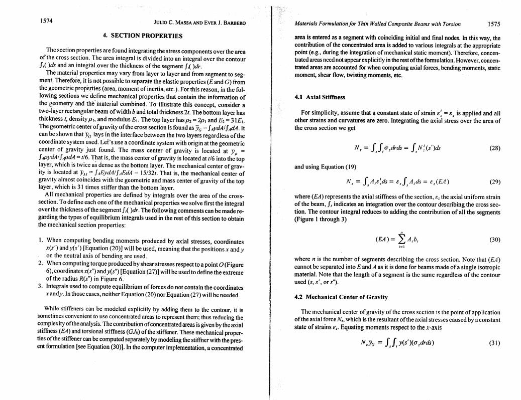
Figure 3. Definition of principal axes of bending for a general open section.

Figure 2. Definition of the local coordinate system, node and segment numbering for (a) aclosed section, (b) and open section.

JULIO C~MASSAAND,EvER J. BARBERO

fMY

tOY,Y

2 1~3I

CD s1 10 I X ax Mx- ---..---.....

zNz~

~44 ,.

1562

The cross section is described by the contour, which is a line going through themidsurface ofall the panels that form the cross section (Figure 1). Each panel is de­scribed by one or more segments. One segment is used for each panel in Figure 2a.Two segments or more are necessary for each flange in Figure 2b because a nodemust be placed at the flange-web connection. From now on we will refer to seg-

Figure 1. Definition of the globaland local coordinate systems, andnode andsegmentnum­bering for a symmetric, closed section.

2. DESCRIPTI(~l~i OF THE CROSS SECTION

box-beams exhibiting bending-torsion 1 coupling, extension-shear' coupling,extension-torsion coupling, and bending-shear coupling,' typical ofhelicopter ro.tor blades. While strong coupled behavior is common in helicopter rotor blades, itis not common in most stn~ctural applications such as civil construction, automo·tive, etc., because coupling leads to undesirable residual stresses and warping dur­ing manufacturing. " '

The objective of this. inve~tigation is to develop simple equations that can beused for design of open ~r closed sections of arbitrary shape. In order to arrive atpractical equations, the off-ply layers should be arranged in a balanced symmetricconfiguration. The laminate can be unsymmetrical as a result oforthotropic layers(isotropic, unidirectional, or random reinforced layers) that are not symmetricallyarranged with respect to the·middle surface.

• *The current computer implementation allows for up to three predefined segments to converge to the initial node"iof any segment (see Table 1 and 2). \

Table 2. Contour definition for Figure 2b.

Segment Number n/ n, Segments Converging to n,

1 1 2 0 0 02 3 4 0 0 03 4 2 2 0 04 2 5 1 3 05 6 7 ..0 0 06 5 7 4 5 0

,1565

NIZ{+)

"

4+,./" .1it.J~~r~

~

s

Thin Walled Composite Beams with Torsion

Figure 4. Definition of stress resultants in the laminate.

Di

NIS<Y

Segment 4 is defined with the common node (node 2) as the initial node. Segments1and 3 must be defined as converging to segment 4, so that the contour integral forthe static moment will accumulate the contribution of the previous segments. Asegment with a free edge can be defined at any time with the free edge as the firstnode (n;) with the exception of segment 6 where the free edge is the final node ofthe segment to complete the contour integral. Note that the local coorqinates areoriented from nj to nj, resulting in opposite orientation in segments 1 and 2. Thishas an important implication in the way the laminate is defined because the firstlayer is always at the surface with negative r-coordinate.

The coordinates of each node are given in terms of an arbitrarily selectedglobal coordinate system. The global coordinate system is shown in Figure 1and Figure 3, with axes z, x,y. In Figure 3, the coordinate system fj,~, rotatedand angle {) with respect to the global coordinate system, describes the princi-

, pal axes of bending.Each segment also has its own local coordinate system (Figure 2). The contour

coordinate s is oriented from the initial node to the final node. The other two localcoordinates are the global z-axis a~d the r-axis that is obtained as the cross productofz tirnes s, or r :::: Z Xs, in such a way that the r-coordinate spans the thickness ofthe segment.

The fiber orientation of layer k is given by the angle <jJk (Figure 4) which is posi­tive counterclockwise around the r-axis and starting from the z-axis. While the

JULIO C. fvIASSAANDEvERJ. BARBERO,

", ", Segments Converging to",

1 2 0 0 02 3 1 0 0

'3 4 2 0 04 ' 1 3 0 0

Table 1. Contour definition' for Figure 2a.

1234

Segment Number

1564

ments instead of pa'nels to' describe each flat or curve wall composing the thinwalled beam because the term panel is used in many engineering disciplines to de­scribe such things as,stiffened panels in ship or aircraft construction, bridge pan­els, etc. The segments can be flat:or curved in the shape ofan arc ofcircle (Figure3). Concentrated areas can be a~ded to represent the contributions ofattachmentsthat we do not choose to mode}, ~"plicitly. Arc segments are divided in a largenumber of flat segments for analysis.

The definition of each segment is done in terms of the nodes, which can benumbered arbitrarily. All. s.~gments are defined by an initial node nj and a finalnode nj. Arc-circular segments need a third mid-node to define the geometry.For a closed section, the segments and the nodes are numbered consecutively.Reference must be made to all the segments converging to the initial node ofeach segment**. Table 1 summarizes the description of the contour shown inFigure 2a. Table 2 summarizes the description of the contour shown in Figure2b.

'-fhe contour integrals are done segment by segment, accumulating the contrib,u­tion ofall the segments. The order in which segments are defined and the orienta­tion ofthe s-coordinate in each segment must allow for the correct accumulation ofcontour integrals such as first moment ofarea, which must start at a free end. Tak­ing Figure 2b and Table 2 as an example, note that the definition ofthe segments 1and 2 start at a free edge with the s-coordinate oriented towards the common node.

z-axis always coincides with the axis ofthe beam, the r-axis orientation dependson the nodes n; and nf. Thefirst layer (k =1), ofthickness r, is located at the bottomofthe laminate, on the ne,gative r-axis. It is important to emphasize that ifone seg­ment orientation is chahged; a) the order of the laminas in that segment must bechanged and b) theisigri of f?ach lamina orientation angle lj>k in that segment must

also be changed. <

1566JULIOC. MASSA AND EVER J. BARBERO Materials Fornzulationfor Thin Walled Composite Beams' with Torsion 1567

-e~ a t6 ,Pit Pt2 PI6 N~all a l2

ei a 22 a 26 PI2 P22 /326 N~ = 0s

y~s a 66 {316 {326 f366 N;s} (2)=

IC~ all 012 016 M:IC: 022 026 M~ = 0

lC~s sym. °66 M:.{

e~ all a l6 fJlI PI6 N:y~... (l16 U 66 fJI6 f366 N:~ ~ (4)=IC~ PII PI6 d 11 d l6 A1;

IC~ ... fJI6 fJ66 d l6 (~ 66 IvfL

which is an approximation. This assumption was also used in Reference [28] to de­velop a theory for laminated thin walled beams ofsymmetric cross-section subjectto bending only. The results of such theory compare favorably with experimentaldata [29] and finite element results [28, 30, 31]. Then, by virtue of Equation (3),the second and fifth column ofthe compliance matrix [Equation (2)] are not used,and retaining only the terms that are of interest we get

Ifthe laminate has off-axis plies that are balanced symmetric, then al6 = f3J6 = o.The term d 16 is zero for laminates made with specially orthotropic layers. When theoff-axis plies are made with intermingled or stitched ±() I~yersoffabric, each layeroffabric is specially orthotropic and l5 16 =0 for the laminate. To reduce manufac­turing costs, 111any cOlnposites are now made with stitched fabrics that contain hvointer-mingled ±9layers in one layer instead ofstacking two layers ofprepreg tape.Then, the laminate is usually made symmetric to avoid warping due to residual

Equations 1 and 2 contain the plane stress assumption ar = O. Next, the unde­formability of the contour is used, as in classical thin walled theory, to further re­duce the complexity ofthe problem. Tsai [26] used the elements ofthe compliancematrix in Equation (2) to define inplane and flexural engineering constants for alaminate, effectively setting all but one ofthe stress resultants in the right hand sideof Equation (2) to define each coefficient. Wu and Sun [27] showed that using theassumption N ~ =M.: =0 for slender, thin-walled laminated beams yields more ac­curate results than the alternative plane strain assumption e~ = IC~ = O. Therefore,we assume

(3)N i = M~ = 0.'1 .'1

Ni All A I2 A t6 B lI B t2 Bt6 e l:

Ni A 22 A 26 B I2 B22 B26 ei

s s

N~s A66 Bt6 B26 B66 y~ ~ (1)=

M~ Dtl Dt2 Dt6 IC':

M i D22 D26 "Is

s

M;s sym. D66 ,,~s

where the superscript (y indicates the segment number, Apq are the inplane stiff­ness, 8

pqare the coupling stiffnesses, and Dpq are the out-of-plane stiffnesses (see

References [24,25]), with p, q = 1, 2, 6.In Equation (1 ), N; ,N.:, and N;s are the tensile and shear forces per unit length

along the boundary ofthe plate (Figure 4) with units [N/m], M:, M:, M~ are themoments per unit length on the sides, with units [N]. The bending moments arepositive when they produce a concave deformation looking from the negativer-axis. The mid-plane strains are e~, e~, and y~." and the curvatures are IC~, IC~, andlC~s . Note that from equilibrium as: = a zs• Therefore, only Mz., will be used in the restof this paper, with the orientation given in Figure 4.

The superscript ( Yis used not only to indicate the segment number but also todifferentiate the plate quantities N:, N;, N:s ' M:, M.:, M:s ' e~, e~, Y~s' IC~, IC~, andIC~ (which vary along the contour, see Figure 4) from the constant beam quantities*N" Q,/, Q~, M

z, Mq, M~, e"" ICq, IC~, andp (see Figure 1) to be defined later. Plate

stress resultants (forces and moments per unit length) and strains are function ofthe contour coordinate s and must be interpreted as N ;(s), N.: (s), e~(s), e~ (s), etc.,

in the rest of the paper.The stiffness equations (Le., ABD matrix) are inverted to get the compliance

equations

,I,

3. SEGMENT STIFFNESS

Each segment of the cross seotion is modeled initially as a thin plate using theconstitutive equations ofalaminated plate, neglecting transverse shear deforma-tion ",~

MiJt~1'ials Formulationfor Thin Walled Composite Beams with Torsion 1569

stresses created during curing of the material. If the laminate needs to be unsym­metrical, it is usually b~cause ofthe addition ofisotropic or 0/90 pairoflayers. Un­der these condition~ O,i6= o. Otherwise, 0)6 decreases rapidly in magnitude whenthe number ofoff-ax:fs, balanced symmetric layers increases [24]. Then, assuminguncoupling bet'reen' norrnal'and shearing effects, the compliance equation [Equa-tion (4)] can be wri~en as

where E; is the equivalent elastic modulus of layer k along the z-direction. Al­though the equivalent modulus E; 'can be computed [24], it is not necessary tocompute this value in order to perform the analysis described here because it issimpler to use Equation (1) through (6) or the static condensation procedure de­scribed previously. Performing the integration we obtain

1568 JULIO C.' MASSA AND EVER J. BARBEROa: = E:(e ~ - r,,;) (8)

Here, D; is the bending stiffness ofthe segment under bending M;, Fi is the in­plane shear stiffness under shear N:s ' Hi. is the twisting stiffness under twistingmomentM~s' and C, is the coupling between the twisting curvature lC~s and theshear force per unit length N~s [see Equation (6)] also called shear flow q. A simple

t~ all PII 0 0 N:"i PII °Il 0 0 M; t: (5)

; =Y.;j' 0 0 a 66, {366 H' , I with

I:s

,,~s 0 0 1366 ~66 M:s""1''.,

Inverting Equation (5) we 'obtain a reduced constitutive equation for the i-th seg­

ment

Taking into account that the behavior ofeach layer (denoted by the superscriptk) in the laminate is elastic, we can write

(9)

(11 )

(10)

N; = A;e~ + B,IC~

1/2 N

A. = f E~dr = " E~tkI -112" .LJ ..

k=)N

f 112 LB. = rE~dr = E~tkrkI -112" ..

k=1

D. = I'12 r2E~dr = ~ E~ [<tk )3 + tk {i;k )2]

I -112" .LJ.. 12k=1

N

f l12 k "k kF; = -112 G;:... dr = .L.J G=..J

k=)

H. = f'/2 r2G~ dr = f G~ [<tk )3 + tk (;Ok )2]

I -112 -" k=)"s 12N

f '12 k ~ k Ie-kc; = -1/2 rGzsdr = .L.J Gzst rk=)

where N is the number oflayers in segment i, t k is the thickness oflayer k, r is the thick­ness coordinate, and rIt is the distance from the middle surface ofthe segment to themiddle surface of layer k (see Reference [24] exercise 4.2.3). Clearly, Ai is the axialstiffuess per unit length ofthe segment. The term B; represents the coupling betweenbending curvature lC~and extensional force per unit length N: that appears when thelaminate is not symmetric with respect to the midsurface ofthe segment. Using the ex­pressions for the remaining stress resultants, it can be shown that

(7). f112N~ = a ~dr

.. -112"

" .

N: A; B; 0 0 e;

M; B; D; 0 0 K.~ ~z

N~= (6)

0 0 F; c; Y~

M:s0 0 c; Hi lC~s

The reduced constitutive equation [Equation (6)] is very important in this work.The segment stiffhesses A;, B;, D;, F;, C;, and H; allow for the detennination ofall thesection properties needed to solve the general problem of bending and torsion. Notethat the beam theory assumptions N.~ = M.: = 0 do not preclude the deformations e~and IC ~ which can be computed from the second and fifth equations in Equation (2).

A convenient numerical procedure to obtain directly the coefficients in Equa­tion (6) is to statically condensate the second and fifth columns of Equation (1)(see Reference [32] pp. 450). A simple and efficient way is to reorder the rows andcolumns in Equation (1) so that the second and fifth rows and columns occupy thefirst two rows and columns. Then, interrupt the Gauss elimination process after thefirst two elements of the diagonal are equal to one.

A simple physical interpretation for the coefficients in Equation (6) can be ob-tained by using the expr~ssion for the stressr~s~ltants. Fore~ample,consider theinplane force per unit length .

3.1 Principal Ax.is o( Bending of the Segment

where E, G, t, b, arid 1 are the elastic modulus, shear modulus, thickness, width,moment of inertia, and JR = bf/3 for the isotropic material.

To investigate the physica~;significanceofthe term Bi, we propose a state ofde­formation E: ¢ 0 with all the ,other strains and curvatures equal to zero. Then, thefirst two of Equation (6) become

(19)

(18)

(17)

1571

(Eli, ) = D.h.s I I

- 2Dj = Dj - ebA;

{:D=[Ad ;J{:]

and the bending stiffness of the segment as

Note that we have multiplied by the segment width hi so that the units of (El) are[Nm2

]. Also note that (El) cannot be separated into E and 1as it is done for homoge­neous isotropic materials.

The symbol (El) indicates a single value (the bending stiffness), not a product ofE times I. Two letters in parenthesis have been chosen instead of defining anewsymbol so that the analogy between the present fonnulation and the case of iso­tropic materials discussed in classical textbooks [33,34] is apparent.

Therefore, the first two constitutive equations in Equation (6) become uncoupled

and using Equation (15), we can write the bending stiffness per unit length ofthesegment as .

: Materials Formulation for Thin Walled Composite Beams with Torsion

(13)

(12)

N~ = AiE~

M~ = BiE~

Ai = Et = EA/b,~,

D; = £t 3/12 =EI/bF; = Gt = GA/b

, 3 1H. =Gt /12 = -GJR/b, 4

that can be solved to give

analogy with isotropic materials indicates that

1570

where

. Bi · .M' = -N' = e N ': Ai z b z

(14)

when N ~, M:, E ~ and K~ ar~efinedwith respect to s' -axis (neutral surface ofbending in Figure 6), with D; given by Equation (17).

Theresultant force corresponding to a strain E: constant through the thickness ofthe segment acts along the axis s' (which is on neutral surface of bending) on apoint with coordinates (see Figure 6)

B ieb =T

I

(15) x(s') = x(s) - eb sin a~

y(s') = y(s) + eb cos a~(20)

gives the location ofthe neutral surface of bending for the segment i. A force N~acting with eccentricity r = eh (axis s') respect to the midsurface (contour s) in Fig­ures 5 and 6, produces no bending curvature K~.

Once the location of the neutral axis of bending is known, the bending stiffnessof the segment is computed with respect to the principal axis s' of the segment(Figure 5 and 6). Assuming that N ~ = 0 and replacing the first equation in Equation(6) into the second equ"tion, we obtain

where a ~ is the angle of the segment with respect to axis x.

3.2 Principal Axis of Torsion of the Segment

To investigate the physical significance ofthe terms C; we propose a state ofde­formation y~.'I ¢ 0 and all other strain and curvatures equal to zero, the last twoequations in Equation (6) also become uncoupled

M: = (n. _(B;)2}..I ---- IA . z

;

(16) N~s = FiY~S; -c ;M:s - iY:...

(21)

that gives the location ofthe neutral axis oftorsion for the segment i. A shear force N :.'iacting with eccentricity r=eq(axiss") respect to the midsurface (contour s) in Figure 6,produces only shear strain which is constant through the thickness. No twisting curva­ture K~s is induced by the lack of symmetry of the laminate in that segment.

Once the location ofthe neutral axis of torsion is known, the torsional stiffness ofthe segment is computed with respect to the principal axis ofthe segment s" (Figure 5).Assuming that N ~s = 0 and replacing the third equation in Equation (6) into the fourthequation, We obtain the torsional stiffuess per unit length of the segment as

1572

Y .YG

XI

XG

G

YG

JULIOC~ MASSA AND EVER J. BARBERO

Y.I IY.

a~!1 I XG

x

Materials Formulationfor Thin Walled ~omposite Beams with Torsion

that can be solved to give

M I- N I

:s - eq :s

with

c/elf = F

I

1573

(22)

(23)

Figure 5. Cross section of segment i showing the definition of the various variables.

y

Hi = Hi - e~Fi

and the torsional stiffness of the segment as

(24)

~henN~s' M~s' Y~s' andK~s are defined with respecttos"-axis (the neutral surfaceof torsion in Figures 5 and 6), with Hi given by Equation (24).

The shear flow corresponding to a shear strain Y~s constant through the thick­ness acts on the neutral surface oftorsion (axis s") on a point with coordinates [seeFigure (6)]

ax'

s'

x

(GJ~ ) = 4Hi b j

where the factor 4 is explained in Section 4.4.1 [see Equation (46)].Therefore, the last two equations of Equation (6) reduce to

{N:; }= [F; ~] {y~}M:s 0 H, K:s

(25)

(26)

Figure 6.. Cross section of segment i showing the definition of the radius R.

x(s") = x(s) - eq sin a~

y(s") = y(s)+eqcosa~(27)

1. When computing bending moments produced by axial stresses, coordinatesx(s') andy(s') [Equation (20)] will be used, meaning that the positions x andyon the neutral axis of bending are used.

2. When computing torque produced by shear stresses respect to a point 0 (Figure6), coordinatesx(s") andy(s") [Equation (27)] will be used to define the extremeof the radius R(s") in Figure 6.

3. Integrals used to compute equilibrium offorces do not contain the coordinatesx andy. In those cases, neither Equation (20) nor Equation (27) will be needed.

The section properties are found integrating the stress components over the areaof the cross section~ The area integral is divided into an integral over the contourIs< )ds and an integral ,oyer the thickness of the segment 1,( )dr.

The material properties may vary from layer to layer and from segment to seg­ment. Therefore, it' is not possible to separate the elastic properties (£ and G) fromthe geometric propextie~ (area, moment of inertia, etc.). For this reason, in the fol­lowing sections we define mechanical properties that contain the information ofthe geometry and the'material combined. To illustrate this concept, consider atwo-layer rectan,gular beam ofwidth b and total thickness 2/. The bottom layer hasthickness I, density pt,;and modulus £1. The top layer hasp2 = 2pI and £2 = 31£1.The geometric center ofgrav'ity ofthe cross section is found as Ya =I A)ldA/f AdA. Itcan be shown that Yo lays in the interface between the two layers regardless ofthecoordinate system used. Let's use a coordinate system with origin at the geometriccenter of gravity just found. The mass center of gravity is located at Yp =

I A{JydA/I A{JdA == 1/6. That is~ the mass center ofgravity is located at t/6 into the toplayer, which is twice as dense as the bottom layer. The mechanical center ofgrav­ity is located at YM ~-= I AEydA/IAEdA = 15/321. That is, the mechanical center ofgravity allnost coincides with the geometric and mass center ofgravity of the toplayer, which is 31 times stiffer than the bottom layer.

All mechanical properties are defined by integrals over the area of the cross­section. To define each one ofthe mechanical properties we solve first the integralover the thickness ofthe segment It( )dr. The following comments can be made re­garding the types ofequilibrium integrals used in the rest ofthis section to obtainthe mechanical section properties:

4.1 Axial Stiffness

(30)

(29)

(28)

1575

(EA)= !Aib;;=1

N. = ffa.drds= fN~(s')ds• s'· s ..

and using Equation (19)

N: = fsA;E~ds = E:f.. A;ds = E:(EA)

where (EA) represents the axial stiffness ofthe section, E: the axial uniform strainof the beam, Is indicates an integration over the contour describing the cross sec­tion. The contour integral reduces to adding the contribution of all the segments(Figure. 1 through 3)

4.2 Mechanical Center of Gravity

where n is the number of segments describing the cross section. Note that (EA)cannot be separated into £ and A as it is done for beams made ofa single isotropicmaterial. Note that the length of a segment is the same regardless of the contourused (s, s', or s").

For simplicitY,assume that a constant state of strain e~ =e;: is applied and.allother strains and curvatures are zero. Integrating the axial stress over the area ofthe cross section we get

area is entered as a segment with coinciding initial and fmal nodes. In this way, thecontribution of the concentrated area is added to various integrals at the appropriatepoint (e.g., during the integration ofmechanical static mOlnent). TIlereforc, concen­trated areas need not appear explicitly in the rest ofthe formulation. However, concen­trated areas are accounted for when computing axial· forces, bending moments, staticmoment, shear flow, twisting moments, etc.

Materials Formulationfor Thin Walled Composite Beams with TorsionJULIOC. MASSA AND EVER J. BARBERO

4. SECTION PROPERTIES

1574

The mechanical center ofgravity of the cross section is the point ofapplicationofthe axial force N:, which is the resultant ofthe axial stresses caused by a constantstate of strains E:. Equating moments respect to the x-axis

While stiffeners can be modeled explicitly by adding them to the contour, it issometimes convenient to ~se concentrated areas to represent them; thus reducing thecomplexity ofthe analysis. The contribution ofconcentrated areas is given by the axialstiffuess (EA) and torsional stiffness (GJR) ofthe stiffener. These mechanical proper­ties ofthe stiffener can be computed separately by modeling the stiflher with the pres­ent fonnulation [see Equation (30)]. In the computer implementation, a concentrated

N;:YG = Is I, y(s')(a :drds) (31)

:',E:(EA)YG = Ez!s(y(s)+eh cosa~)Aids (32)

1576

and using Equation

JULIO C~MASSA AND EVER J.BAlWERO. . . . . . . .. ,·.·Mat~rials Formulationfor Thin Walled Composite Beams with Torsion

(E/:,) == (EI~, )cos2a~+ (E/:, )sin 2 a:(£1~,)= (E1~, )sin 2 a: + (£1:, )cos 2 a~

(£1;,/ ) = [(EI:, ) - (£1.:, )] sin a~ cos a~

1577

(36)

Finally, using the parallel axis theorem and adding the contributions of all thesegments, we obtain the mechanical moments of inertia and the mechanical prod­uct of inertia with respect to axes XG, YG,

where Xi, Yi are the coordinates of the center of segment i (point P in Figure 5)over the contour s (r =0) with respect to the global system XG,YG. The systelTI Xc,

YG has its origin at the mechanical center ofgravity ofthe section and it is paral­lel to the global system x,y. In Equation (37), (Xi - eh sin a~) and (y; + eh cos a~)are the coordinates of the center of the segment (point P' in Figure 5) over theaxis s' (r = eh).

The rotation it locating the principal axes of bending 'YJ, ~, with respect to theaxes xG, YG, is found as usual by imposing the condition (EI,,~) = 0

Solving fQr Yc and repeating the same procedure for xG

we obtaini .,

(ES x )

YG = (EA)

(ES), )

xa = (EA)

where (ESx) and (ESy ) ar~. Hie mechanical static moments defined as

.. (ES x )= !,Y(s')A/ds= fy/A/b j

i=)II

(ES y ) = !o;x(s')Aids = LxiAibi;=)

and Xi' Yi' are the coordinates of the point P' (Figure 5) where s =b;/2.

4.3 Principal Axes of Bending of the Beam

(33)

(34)

(El xc; ) = I [(EI;. ) + Aib/ (y/ + eh cos a~)2];=1

(El yG )= I[(E/~.')+A/b;(Xj- eh sina~)2]i=1

(EIX(iYr, ) = f [(EI:.... ) + A jbj (Yj + eh cos a~ )(x/ - eh sin a~)];=1

(37)

The product of the modulus of elasticity E times the moments of inertia !y, I)',and the product of inertia Ixy ofclassical beam theory are replaced by the Inechani­cal properties of each segment defined as

tan 2i} = (38)

Note that the bending stiffness (EI.:,) was derived before [Equation (18)] andthat the mechanical product ofinertia (El :'.~' ) van ishes because the s'r' are the prin­cipal axes ofbending ofthe segment (Figure 5). The mechanical moments ofiner­tia and the mechanical product of inertia of a segment with respect to axes x'y'(Figure 5) are obtained by a rotation-a~ around Z, as Taking into account the uncoupling between shearing and torsional effects in

and the maximum and minimum bending stiffness with respect to the principalaxes 'of bending are

(EI.:' ) = D;bi

. b~(El', ) = A. -!-.

r , 12

(El:,s') = 0

(35)

.. _ (ElxG)+(EIYG)+J(ElxG)+(EIYG))2 . 2(EI" ), (£1 f: ) - - + «Elx )" »

s 2 2 G&

4.4 Torsional Stiffness

(39)

Energy balance implies that the work done by external torque equals the strain en-ergy due to she,ar " '

(46)

1579

(GJR ) = 4t Hlb,; .... 1

Wal/ed,~o",posite.Beams with Torsion

TIp is the torsional stiffness (GJR), we have

For the isotropic case, Equation (46) leads to JR = 1/3~b;t:.

4.4.2 SINGLE-CELL CLOSED SECTIONIn this case IC::s = 0 and Equations (40) reduce to

(40)

l, JULIO,C.',MAsSAAND"EVER,J.BARBERQ'"

qJ = F,,,~,v

M:s = HiIC~.<;

1578

Equ'ation (26) when using prinqipalaxis of t()rsi011, S"tan~noting thatshear flow qi we have ' ," " '

4.4.1 OPEN SECTION:For the open section, the shear flow vanishes{q =0), so Equ8tions (40) reduce to

where pis the rate oftwist.' Ffum Equation (40) and (41), it is possible to derive thetorsional stiffness for botli' t~e open and closed section using the kinematic as­sumptions of the classical theory.

Note that the superscript i has been dropped from ICzs because the twisting curva­ture is unique for the section while the twisting moment varies from segment tosegment. For the open section, the twisting curvature of classical plate theory istwice the twist rate p

(47)

(49)

(48)

(50)Tf3 = q2~ ds·~Fj

qi = F;y~s

M:s = 0

Tp = gssY~sqids

The energy balance [Equation (41)] reduces to

Equilibrium ofmoments can be used to obtain an expression for the torque Tbyintegrating the shear flow' over the contour s"

Replacing Equation (47) in Equation (49) and taking into account that for aclosed cell q is constant along the contour, we have(42)

(41)

q' = 0

M~,~ = HjIC zS

1 Lf" .."2 TP~ ="2 s("~sq' + M~K~ )<Is

where wis the transverse deflection ofthe laminate. The energy balance [Equation(41)] can be written

The torsional stiffness is obtained dividing Equation (51) by Equation (52)

T = ~ (qR(s"))ds = q[2fs.] (51)

q ~ dsf3=-~- (52)

E s• F;

(53)T [2f

Jo ]2

(GJR)q = P= ~:' !!.!..LJ,=lF;

where r.~.. is the area enclosed by the contour s".The rate of twist f3 is determined dividing Equation (50) by Equation (51)

(45)

(43)

(44)

d 2W

K =2- = 2{3zs dZdS

TP= 4Is H I ds

Tf3 = Is H;IC;sds = IC;s Is H;ds

and using Equation (43). we have

1580 JULIO C. MASSA AND EVER J. BARBERO Materials Formulation/or Thin Walled Composite Beams with Torsion 1581

The expression above can be improved to account for the nonunifonn distributionof shear through the thickness of the laminate. This is done by adding the torsionalstiffhess ofthe open cell affected by a correction factor equal to 3/4 (see Appendix)

The analysis ofshear stiffness, sectorial properties, shear center and restrainedwarping, must be considered separately for open and closed sections. To obtainthese expressions, we must consider the shear flow caused by shear forces. As inthe case of homogeneou~111aterials, the shear flow caused by shear forces is ob­tained as an equilibrium condition using Jourawski's fonnula. But in the case ofinhomogeneous materials, according to Equation (15) and (23), the resultant ofax­ial forces that causes no bending curvature, and the resultant of shear flow thatcauses no twisting curvature act on different local axis. The same situation occursin the case of restrained warping.

Note that consistently with classical thin wall beam theory, eccentricity ef­fects eh and eq could be ignored, assuming the wall to be very thin. However, us­ing eh and eq along with a linear variation of all the strains through the thick­ness, as provided by classical lamination theory [Equation (1 )], it is possible toimprove upon classical thin walled theory, modeling the thickness effects formoderately thick walls. Therefore, we will use the notation 1](s'), ~(s'), r(s"),etc., [Equation (20) and Equation (27)] to indicate on what local axis the globalcoordinate is measured.

(ES ~ (s» = f;1](s')A j ds = f:(1](s) - eh sin a~, )A ids (56)

Equation (58) is used to compute the consistent bending stiffness to be used inJourawski's formula [Equation (57)]

(59)

(58)

(57)

(EI;)* = - fs(ES~ (s» cos a~/ds

q,/ (s) = -Qq (ES~ (s)(El ~ ) *

f . -Q" f .Q" = (q" (s)ds)cos a:, =--- (ES~. (s» cos a;,dss (EI ~ ) * s

Integrating the forces originated by the shear flow we have

Similarly

where a~, is the angle ofthe segment with respect to the principal axis 1]. This inte­gral must start at the free end where s = O. Note that the mechanical static moment(ES~(s» defined in Equation (56) is variable along the contour,while the values de­fined in Equation (34) are the total values for the beam cross section.

Integrating the shear flow caused by Q", and using Equation (55), we do not re­cover exactly Q". The difference grows with the thickness. A better approximationto q,,(s) can be obtained by defining a consistent bending stiffness (EI;)* to be usedin Equation (55) so that equilibrium is satisfied

(54)',", (OJ ) = [2I"s' ]2 + ~ [4~ H.b.], . R ~11 b. 4 LJ ", LJ -!- ;=1

. /=JF/

4.5 Shear of Ope~Sections

4.5.1 SHEAR FLOW CA USED BY SHEAR FORCESUsing principal axes ~, 1] (Figure 3), the shear flow caused by a shear force Q" is

given by Jourawski' s fonnula (Reference [33] pp. 361) adapted for non homogeneoussections by replacing geometric properties by the mechanical properties used in thiswork. The first moment ofthe area at one side ofthe point where shear is evaluated isreplaced by the mechanical static moment (ES~(s». The moment ofinertia is replacedby the bending stiffuess (Eh), defined in Equation (39). Then, the shear flow is

where

q/J~) = -Q~ (ES 11 (s»)(EI )*

'I

(ES" (s» = f:(~(s) + eh cos a~ )A;ds

(60)

(61)

qq(S)= -Qq(ES~(s»(EI; )

(55) (El" )* = - f (ES" (s»sin a~/ds.f

(62)

where Q" is the shear force applied in the direction 1] (Figure 3) and (ES;(s» is themechanical static moment which is variable along the contour

Equations (59) and (62) are used to compute a consistent bending stiffness toimprove Jourawski's formulas [Equation (57) and (60)]. This correction is gener-

(70)

(69)

(68)

(71)

(Ew) = Is w(s)A;ds

(Elw) = fs[W(S)]2 A;ds

(ESw~)= Is (7](S) - eb sin a~ )w(s)Aids

(ESw,,) = fs(~(s)+ eb cos a~ )w(s)A;ds

The mechanical sectorial linear moments

The. mechanical sectorial moment of inertia

1583

4.5.4 MECHANICAL SHEAR CENTERThe coordinate ~c ofthe mechanical shear center is calculated by equilibrium of

moments (with respect to the mechanical center of gravity), caused by the shearforce Q'1 and its associated shear flow qq(s) [defined in Equation (57)]

SH because dw(s) will be used to define twisting moment caused by shear flow (act­ing on sIt) in Equation (72) through Equation (76).

In the case ofopen sections, Equation (67) may require to treat the segments in adifferent order ofthat used initially to define the contour (Table 2), because we canstart to compute a segment only if the value of w(s) in either extreme is alreadyknown. InFigure 2(b), we add sequentially the static moment ofsegments 1,2,...,6.To compute sectorial area the order is 1, 3, 2, 4 ...6.t

The sectorial area w(s) is used in the,definition ofthe mechanical sectorial prop­,erties, which are defined as follows:

The mechanical sectorial static moment

(65)

(63)

(GAq

) = [(Elq )*]2

IJ(ESq (s»f ds (66)F,

(GA~ ) = [(El~ )*]2

IJ<ES ~ (s»]2 dsF i

, . , 2

, 1" ,'., 1 Q" 1I I I I I

2. Qq'Ydz =2. (GA ) dz =2. s(M.,J':s + q 'Y:s ) dsdz. ~

Similarly

. qi -Q'1(ES~(s))

'Y~s = F; = F;(El~)*

Replacing into Equation (63) with K~ == 0, owe obtain the shear ,stiffness ofthe ,section as

While the straineriergy is computed as an integral over the volume, it must benoted that the integra'l ov:er the thickness has already been computed in Equation(6). Taking into account Q111y the shear deformations (IC~. == 0), and using the third'of Equation (6) and Equatio~ (57) we have .

4.5.2 SHEAR S·rlFFNESS OF THE SECTIONFor an infinitesimal segment dz ofthe beam subject to shear Q", the balance be­

tween the external ~ork and the strain energy is

ally overlooked in the literaturefor:the;isotropi~case~butjt is necessary tor thecase of beams with moderately thick walls.

1582

tThe current computer implementation reorders segments automatically.

where the initial point I is at the free end and F is the final point(Figure 2). UsingEquation (57) and (56) into (72) we have

4.5.3 SECTORIAL PROPERTIESThe sectorial area is defined in the usual fonn (Reference [33] pp. 307)

w(s) = I:R(s")ds (67)

using arbitrary points for the pole and for the initial point where w(s) =0 (Figure2). The radius R in Equation (67) (see Figure 6) must be evaluated on the local axis

l: fF "Q,/r; C = J R(s )q,/ (s)ds (72)

where w(s) is the principal sectorial area as will be shown in the next section. Equi­librium of forces requires a secondary shear flow

The pole ofthe sectorial area w(s) is the mechanical center ofgravity because inEquation (72) the moments are taken respect to the point (xG, YG). Similarly

(82)

(80)

(83)

(81)

(84)

(79)

(85)

J585

Is "w1(s)= R(s )dsJ -

Is w(s)A;ds = 0

N: = f .. N:(s)ds = 0

(Elw) = fs[W(S)]2 Aids

d 4() 2 d 2

(} 2 T'--k -=-k -dz 4

dz2 (GJ R )

Is (1](S) - eh sin a~ )w(s)A;cb' = 0

Is (~(s) + eb cos a~1 )w(s)A;ds = 0

The angle of twist () is computed solving the general equation for torsion

The bending moments Me and M,I caused by the secondary axial forces must alsovanish. Using Equation (77), the conditions M~ = 0 and A1'I = 0 lead to

These equations can be satisfied, using an arbitrary initial point, ifthe mechani­cal shear center is used as a pole. As it was seen at the end ofSection 4.5.4, the lefthand side of Equation (83) and (84), which are nlechanical sectorial linear mo­ments [Equation (69) and (70)] will vanish. To satisfy Equation (82) the initialpoint is changed, which is equivalent to subtracting a constant. To obtain the prin­cipal sectorial area w(s), a sectorial area Wl(S) with an arbitrary initial point is cal­culated first. The mechanical shear center is used as the pole to also satisfy Equa­tion (83) and (84)

and using Equation (77)· leads to

where T' = dT/dz, and fil = (GJR)/(EIW), and (EIW) is the mechanical warping stiff­ness defined as in (Reference [33] pp. 320) which is computed as in Equation (71)but using principal sectorial area

Materials Formulationfor Thin Walled Composite Beams with Torsion

Principal Sectorial Area Diagram. In the case oftorsion Tacting alone, the sec­ondary axial forces integrated in the contour s' must vanish because no axial forceN: is applied

(78)

(77)

(76)

(75)

(73)

(ESw'/)

1] c =- (EI'I ) *

(ESwe)~c = - (EI~)*

d 2(}N;:(s) = - dz 2 w(s)A J

d 3(J sqw (s) = dz3 Iow(s)A/ds

~ _ - 1 fF "[fS ]_ c - (EI~) * I R(s) /7(s')A/dsJds

JULIO C. MASSA AND EVER.). BARBERO

-1 IF [Is] -1 IF=-- s'A. dwds= s'A.wsds 74~ C (EI) * J 1/( ), J (EI ) * J 1/( ) , () ()~ " e

4.5.5 RESTRAINED WARPINGSecondary Forces. When free warping due to torsion is restrained, axial secon-

dary forces appear. They can be computed (Reference [33] Section 8.11) as

It is important to note that ifwe use the mechanical shear center as pole, then ~c =

oand 1]c = o. Therefore, by Equation (75) and (76), the mechanical sectorial linearmoments are zero.

and using Equation (69) ~\'~., ,

Recognizing tn~t.[ft(s")ds] is the differential 'of sectorial area dw(s) and that[1](s')A;ds] i~ th~ differential of mechanical static moment d(ES~(s)), the order ofintegration can be changed (integration by parts). Since the mechanical static mo­ment is zero atthe end points we have

1584

where, as in Equation (67) the end ofthe radius Rls located on the axis s" (Figure6). Then, the principal sectorial area w(s) is defined as

where theconsttult'·~o.is obtained after introducing Equation (86) into Equation(82), or r·· .. .

4.6 Shear of Single Cell Closed Section

4.6.1 SHEAR FLOW QAUSED BY SHEAR FORCESFor closed sections, the point at which q(s) =0 is not known a priori. Therefore, to

use Jourawski' s fonnula. [Equation (57)], it is necessary to proceed in two steps. First,consider the shear force Q" acting on the mechanical shear center which does not pro­duce shear flow by torsion, and apply Equation (57) using an arbitrary initial point.

(95)

(94)

(93)

(92)

1587

q~ (s) = q~ (s) + qo~

q~(s)= _ Q~(ES'/(S»(El )*

'1

~ ds jA\ dsqo~ =-~~qr~(s)F. "JJsF

I I

Q,,~C ='~q'l(s)R(s")ds

··Similarly, the shear flow caused by Q~ can be obtained as

4.6.2 MECHANICAL SHEAR CENTERThe coordinate ~c ofthe mechanical shear center is calculated by equilibrium of

moments (with respect to the mechanical center of gravity), caused by the shearforce Q" and its associated shear flow q,,(S) (Figure 6)

and

where

..··,····(;:·Malertals Formulationfor Thin Walled Composite Beams with Torsion

(88)

(86)

(87)

JULIO C. MASSA AND EVERJ. BARBERO

w(s) = w1(s)- Wo

qlq (s) = _ Q~ (ES ~ (s»(EI~ ) *

w - I fo-(EA) .fW, (s)A;ds

1586

To change the initial point is equivalent to add a constant qo" such that

q" (s) = qltl (s) + qo" (89)or using Equation (89)

where qrll(s) is given by Equation (88) and qO/' is given by Equation (91). Similarly

Since the shear load was applied at the mechanical shear center, the constant qOllmust be such that the section does not rotate due to torsion. The rate oftwist due totorsion is given by Equation (52). Since the shear flow due to shear [Equation (89)]is not constant, we have (see Reference [33] pp. 371)

~C = QI ~,(qbl(S)+qOII)R(s")ds'I

(96)

4.6.3 SHEAR STIFFNESS OF THE SECTIONThe derivation is similar to that ofEquation (63-66). However, for the closed sec-tion, the point where the mechanical static moment is zero is not known a priori.This problem is addressed similarly to Section 4.6.2. For the case ofa unit appliedshear load Q" = 1, Equation (63) leads to

Settingp=0 leads to

1 ~ dsP= 2f ~ ~(qb1(s)+qo,,) F.

s I

~ dS/~dSqOll = -~qltl(S) F. "JJsF.

I I

(90)

(91)

117 C = -Q ~(qr~ (s) + qo~ )R(s")ds

~

(97)

where it was assumed that lC~s = 0 and y~s = q/F; as it was done in Equation (64),q,,(s) is defined 'in Equation (89), and q~(s) is defined in Equation (92)~

where (GJR) is given by Equation (54), (GJR)q is given by Equation (53), (GJR)svisgiven by Equation (46) and the correction factor 3/4 for a circular tube is used as inEquation (54). Introducing Equation (101) into Equation (100) yields

Equation (99) applies for very small thickness. When the thickness is not that small,a better resu It can be obtained recognizing that part ofthe moment is in equilibrium be­cause ofthe Saint Venant stresses, like in the open section. The total torsional moment(1) is distributed among shear flow (Tq) and the Saint Venant stresses (Tsv)

1589

(104)

N:E: = (EA)

M"IC" = (EI,,)

M~

IC~ = (EI~)

rf3 = (GJR)

where the last term correspond to restrained warping [Equation (77)] for an open

. N. M"

M~ d 2(Je~(s) =_. + ~(s)-- -,,(s)-- - -2 w(s) (105)• (EA) - (EI" ) (E/~ ) dz

6. SEGMENT DEFORMATIONS AND STRESSES

5. BEAM DEFORMATIONS

The axial strain in the midsurface at any point can be computed in terms of thebeam deformations [Equation (104)]

Ifthe beam is a component ofa structural system (indeterminate or not), the me­chanical properties (EA), (EI,,), (EI~), (GA,,), (GA~), and (GJR), can be easily trans­formed into equivalent geometrical properties (dividing by arbitrary equivalentmodulus E and G). The nodal displacements ofthe structure and stress resultants atany section can be obtained using the equivalent properties as input for any struc­tural analysis program, either a beam finite element analysis or a matrix structuralanalysis program. Later on, these stress resultants can be used in Equation (104) tocompute the beam deformations at any section ofthe structure. The proposed the­ory and its computer implementation can be used as a pre- and post-processor forany standard matrix structural analysis program.

It is important to note that in.the case ofan isotropic circular tube, the theory de­veloped here [Equation (54), (103),{107), etc.) gives the exact result for stiffnessand strength regardless of the thickness.

The deformations of the beam are now computed using the classical formulasreferred to the principal axes. Therefore, the axial strain E;, the two curvatures IC",

IC~, and the twist ratio f3 are computed as follows

, Materials Formulationfor Thin Walled Composite Beams with Torsion

(98)

(99)

(100)

(101)

(102)

(103)

Tqr = 2f II

S

JULIO C.' MASSA AND, EVER,]., BARBERO

(GA~ ) =1/~ [qq (S)]2,\' F ds

;

(GA,,) = I/~ [q~ (sW.'1 F. ds,

_.I-[ _,_3 (GJR)SV]qr-2f.

14(GJ

R)

s

J\ '~

T=Tq +T.5V

T TsvT q_--= - 3(GJR ) (GJR)q "4(GJ

R)SI'

J:, = T - T."tv = r[l- ~ (GJ R )sr]4 (OJ/()

Recognizing that Tq produces qr in Equation (99), we have

The distribution is proportional to the respective stiffness, according to

1588

4.6.4 SHEAR FLOW CAUSED BY TORSIONThe shear flow due t~ torsion is obtained from Equation (51)

wherea:, is the angie ~e~een the segmentwith i orientation and the principal axis1].

The twisting curvatute, constant for all segments, is calculated from the twist ratep

where the minus sign is .introduced to account for the definition of the positivetorque Tin Figure'l"and the positive twisting moment M~ in Figure 4.

To detennine the shear strain ,,~s (s~ we need first to obtain the total shear flowfrom shear, torsion, and restrained warping, acting in the local sIt axis

section. Note that E~(s) changes point to point because ~(s) and rJ(s) are the coordi­nates in principal axis of a point in the contour s, and w(s) also changes with s.

The bending cu~ature,which is unique for each segment, can also be computedin terms of the ~~,am deformations [Equation (104)]

1591

(110)N~s = q(s)

M:... = eqq(s) + HilC~,..

7. NUMERICAL RESULTS

Numerical results obtained using the procedure developed in this paper arecompared in this section to experimental results from the literature. Experimentalresults for rectangular tubes made of Graphite-Epoxy are reported in Reference[22] and analyzed in Reference [23]. They present results for a box beam of lengthL = 76.2 Cln, clamped at one end and with a tip torque T= 0.113 Nm applied at theother end. The external dimensions of the cross section were: height d = 26.035mIn and width c =:= 52.324 mm. The lanlinate ofall walls \-vas a cross-ply with 6 lay­ers, each 0.127 mm thick, in a [0/90]3 configuration, with a total thickness of 0.762mm. The elastic properties ofeach plywereEL = 141.865 GPa, Er = 9.784 GPa, GLr

=5.994 GPa, and VI,T= 0.42. Note that the laminate is not symmetric but the crosssection is symmetric since the interior layer has the same angle in all walls ofthecross section. While, the reported experimental angle of twist at the tip was 0~420

10-3 rad., the model developed in this paper predicts 0.426 10-3 rad., with a 1.4°A,difference.

Experimental results for lam inated circular pipe are presented in Reference [21 ]along with analytical and finite element analysis ofthe circular pipe. The pipe wasconstructed of 30 layers, each 0.254 mm thick, of hand lay-up fiberglass and ar­ranged in a cross-ply unsymmetricconfiguration [0/90]15. The material propertieswere reported as EL = 16.605 GPa, Er = 7.028 GPa, GLr = 2.315 GPa, and VLr =

Equation (1) is derived under the assumption of linear strain distribution throughthe thickness. While classical thin walled beam theory can account for bending ef­fects, the shear strain caused by torsion in closed cells is constant through the thick­ness, which limits the formulation to thin walls. On the other hand, the present fonnu­lation provides a better approximation by using a linear distribution ofshear throughthe thickness. Therefore, it is possible to analyze moderately thick walls, which are notso thick as to require the inclusion of transverse shear effects. However, the shearstress distribution in the walls due to shear forces [q,,(s) + q~(s) in Equation (108)] arestill considered constant through the thickness.

Materials Formulation for Thin Walled Composite Beams with Torsion

the failure criteria. Three failure criteria were implemented in this work: the maxi­mum stress, maximum strain, and Tsai-Wu quadratic interaction criteria. Thesecomputations are repeated for as many points in each segment of the contour asnecessary to verify that the stresses do not exceed the allowable values.

It is interesting to note that using Equation (107) and (109) in the third andfourth equation of Equation (6) we get as expected(106)

(107)

(108)

(109)

JULIO C. MASSA AND EVER J. BARBERO

IC~ = lC 'I cos a:,+ ICg sin a:,

q(s) = q" (s) + q~ (s) + qr + qw (s)

, i ",. {-2TI(GJR ) open.· section}" c=, .

:~. ,w -T/(GJR) closed section

. N!s - C;,,~ q(s) i i,,' (s) =. = -. - e ".

zs F; F; q.5

1590

where the last term in Equation (108) correspond to a restrained warping [Equa­tion (78)]. The shear flow q'I(S) due to shear forces Q" is given by Equation (57) andEquation (89) for open and closed sections respectively. The shear flow q~(s) dueto shear force Q~ is given by Equation (60) for open sections and Equation (92) forclosed sections. The constant flow due to torsion qT is given by Equation (103) forclosed sections and qr = 0 for open sections.

The shear strain y~.~(s) in the midsurface can be calculated from the third equa­tion in Equation (6)

where q(s) is given by Equation (108) and lC~s is given by Equation (107). Note thatthe shear flow acting ~n s" does not produce curvature; the curvature in Equation(109) is due to torsion only.

Finally, the stress resultants are computed at each point by Equation (6). Thefour stress resultants are complemented withN.: == 0 and M: =0, reordered, and in­troduced in a standard laminate analysis program [using Equation (I)] to evaluate

0.2403. The mean radius ofthe pipe was R= 5.334 em and the length L == 1.219 m.It should be noted that nonlinear behavior was observed for high values oftorque.However, with an applied torque of 1356 Nm the material remained in the linearrange. Under these conditions, a twist' angle of 5.77 degrees was Ilteasured and5.60 degrees was 'predicted using the theory in this paper, with a 3% difference.Also for 13.56 Nmof applied torque, a shear strain of 3675 microstrain (mi­crostrain = '10-6mm/mm) was measured on the surface of the pipe. The analysispresented in· Ref~rence [21] predicted a shear strain of 4316 microstrain while4278 microstrain' was. predicted at the mid-surface using the theory in this paper.The strain at the outer surface can be computed as Y:s + lC:s 1/2 =4580 microstrain.The discrepat:lcy between experimental and theoretical strains may be caused byuncertainties in the J;l1aterjal properties.

1592 JULIO C. MASSA AND EVER J. BARBERO Materials Formulation/or Thin Walled Composite Beams with Torsion

n 2 2(GJR )exacl =4 Dt(D + t )G

with the result for a thin walled tube obtained using Bredt fonnula [33,34]

n· 2(OJR )Bredl = - Dt(D )0

4

and the formula for a tube with a longitudinal slit (open section)

4 [1r 2](GJR )ope" = 3" 4 Dt(t )G

1593

,Il

, 8. CONCLUSIONS

The concept of mechanical properties was introduced in this paper to substitutethe product of the modulus of elasticity times the geometrical properties used inclassical textbooks. With certain care to model the laminated structure ofthe mate­rial, it was shown that it is possible to follow closely the theory ofbeams presentedin classical strength ofmaterials textbooks. This has the advantage that thin-walledcomposite beam theory becomes accessible to a large number ofengineers that arefamiliar with the subject. By transforming the mechanical properties into equiva­lent geometrical properties (dividing by arbitrary values of E and G), the presentformulation can be used as a pre- and post-processor ofany matrix structural analy­sis program. All the contour integrals are reduced to summations over the numberofsegments, allowing for a general solution for any geometry of the cross section,open or closed, without the need for specialized evaluation of contour integrals.Comparisons with experimental data show good correlation, consistent with the as­sumptions of the theory. The formulation presented in this paper can be easily ex­tended to multicell sections and closed cells with fins. Finally, constrained warpingof closed cells can be easily added, although it is usually negligible.

APPENDIX. CORRECTION TERM IN EQUATION (54)

In Equation (49), the shear str~iny:,f is constant through the thickness because ofthe assumptions ofclassical plate theory [24]. For an isotropic section. this trans­lates into i:s :=: constant, which is conltnOn Iy accepted in til in \valled theory. For theparticular case ofa tubular section, the exact solution oftorsion is available, and itreveals a linear variation of'l':.~ through the thickness. Comparing the exact solutionfor the tubular section of mean diameter D and thickness t

it is clear that the thin walled solution for closed tube is missing 3/4 ofthe open sec­tion solution to reach the exact solution for the tube.

REFERENCES

I. Barbero, E. J., Applications: Construction, in Lubin's Handbook of Composites, 2nd. Ed., StanPeters, Editor, Van Nostrand, Reinhold, N. Y., 1998.

2. Savoia, M. and Tul1ini, N., Torsional Response of Inhomogeneous and Multilayered CompositeBeams. Composite Structures, 25(1993) 587-594.

3. Muskhelishvili, N. J., Some Basic Problems ofthe Theory ofElasticity, 4th Ed., Noordhoff, TheNetherl ands, 1963.

4. Cheng, S., Wei, X., and Jiang, T., Stress Distribution and Deformation of Adhesive-BondedLaminated Composite Beams, J. Eng. Mech., ASCE, 115 (1989) 1150-1162.

5. Lekhnitskii, S. T., Theory ofElasticity ofAnisotropic Elastic Body, Holden-Day, San Francisco,CA,1963.

6. Whitney, J. M. and Kurtz, R. D., Analysis of Orthotropic Laminated Plates Subjected to Tor­sional Loading, Composites Engineering, Vol. 3, No I, pp. 83-97, 1993.

7. Whitney, J. M., Analysis ofAnisotropic Laminated Plates Subjected to Torsional Loading, Com­posites Engineering, Vol. 3, No 6, pp. 567-582, 1993.

8. Skudra, A. M., Bulavs, F., Va., Gurvich, M. R. and Kruklinsh, A. A., Structural Analysis ofCom­posite Beam Systems, Technomic, Lancaster, PA, 1991.

9. Sankar, B. V., Beam Theory for Laminated Composites dnd Application to Torsion Problems, J.Appl. Mech., ASME, 60 (1993) 246-249.

10., Tsai, C. L., Daniel, I. M., and Yaniv, G., Torsional Response of Rectangular Composite Lami­nates, 1. AppI.Mech., ASME, 57 (1990) 383-387.

II. Vasiliev~V. V., 1993, Mechanics ofComposite Structures, Taylor and Francis~ Bristol, PA.

12. Hong. C-I-I. and Chopra. I.. Acroelastic Stahility Analysis ora Composite Rotor Bladc~ 1. Amcr.Ilclicoptcr Soc. 30(2), 1985.

13. Librescu, L. and Kehdir, A. A., Aeroelastic Divergence ofSwept-Forward Composite Wings In­cluding Warping Restraint Effects, AIAA Journal, 26(11), 1988.

14. Reissner, E. and Tsai, W. T., Pure Bending, Stretching, and Twisting ofAnisotropic CylindricalShells, J. Appl ied Mechanics, 1972.

15. Mansfield, E. H. and Sobey, A. J., The Fibre Composite Helicopter Blade; Part I: Stiffness Prop­erties; Past II: Prospects for Aeroelastic Tailoring, AeronauticalQuarterly, 30(2), 1979.

16. Rehfield, L. W., Altigan, A. R., and Hodges, D. H., Non-Classical Behavior of Thin-WalledComposite Beams .~i~h Closed Cross Sections, 1 Amer. Helicopter Society, 35(2), 1990.

17. Bachau, O. A., A Beam ~heory for Anisotropic Materials, J. Appl. Mech., Vol. 52, 1985.18. Libove, C., Stresses' and Rate of Twist in Single-Cell Thin-Walled Beams with Anisotropic

Walls, AI¥ l~' Vot 26, '1988.19. Bicos, A. S. and Springer, G. S., Design ofaComposite Box Beam, J. Compo Mater., Vol. 20, 1986.

20. Minguet, P. and'Duguridji, J., Experiments and Analysis for Composite Blades Under Large De-flections; Part I: Staties;Part II: Dynamics, AIAA J., 28(9), 1990. "

21. Zhao, Y. and Pang;S; S., i995, Stress-Strain and Failure Analyses ofComposite Pipe Under Tor­sion, 1 Pressure Vessel Technology, 117 (August), 273-278.

22. Chandra, R.,.Stemple, A. D. and Chopra, I., 1990, Thin-Walled Composite Beams Under Bend­ing, Torsional, and ~xtensional Loads, Journal of Aircraft, 27(7).

23. Smith, E. C. and Chopra, I., 1991, Formulation and Evaluation ofan Analytical Models for Com­posite Box-Beams, J. of Amer; Helicopter Society, 23-35, (7).

24. Jones, R. M., 1975, Mechnnics of Composite Materials, Taylor and Francis, Bristol, PA.25. Barbero, E. J., 1999, Introdu~tion to Composite Materials Design, Taylor and Francis, Bristol,

PA.26. Tsai, S. W., 1988, Composites Design, Think Composites, Dayton, OH.27. Wu, X. X. and Sun, C. T., 1990, Vibration Analysis ofLaminated Composite Thin Walled Beams

Using Finite Elements, AIAA Journal, 29,736-742.28. Barbero, E. J., Lopez-Anido, R., and Davalos, J. F., Mechanics ofLaminated Beams, J. Compos­

ite Materials, 28(8), 806-829, (1993).29. Lopez-Anido, R., Davalos, 1 F. and Barbero, E. 1 "Experimental Evaluation of Stiffness of

Laminated Composite Beam Elements under Flexure," 1 Reinforced Plastics and Composites,14(4),349-361, (1995). I

30. Davalos, J. F., Salim, H. A., Qiao, P., Lopez-Anido, R. and Barbero, E. 1, "Analysis and DesignofPultruded FRP Shapes under Bending," Composites Part B, 27B, 295-305, 1996.

31. Davalos,l F., Qiao, P., and Barbero, E. 1, Muitiobjective Materials Architecture OptimizationofPultruded FRP I-Beams, Composite Structures, 35(3),271-281, 1996.

32. Bathe, K-1, 1982, Finite Element Procedures in Engineering Analysis, Prentice Hall, New Jer­sey.

33. Cook, R. D. and Young W. C., 1985, Advanced Mechanics ofMaterials, Macmillan, New York.34. Boresi, A. P., R. J. Schmidt, and Sidebottom, O. M., 1993, Advanced Strength of Materials, 5th

Ed., Wiley, New York.35. Young, W. C., Roark's Formulas for Stress and Strain, McGraw Hill, N. Y., 1989.

1. INTRODUCTION

(Recieved October 24, 1997)(Revised March 28, 1998)

1595Journal of COMPOSITE MATERIALS. Vol. 32, iVO. 1711998

0021-9983/98/17 1595-22 $10.00/0© 1998 Technomic Publishing Co., Inc.

• Author to whom correspondence should be addressed.

Experimental Evaluation of RepairEfficiency of Composite Patching by ESPI

TSANN-BIM CHIOU

National Nano Device LaboratoriesNational Science CouncilHsinchu, Taiwan 30043

Republic ofChina

KEY WORDS: electronic speckle pattern interferometry, stress intensity factor, compos­ite patching.

ofmanufacturing or applications, damages are occasionally pro­~uu"''''u in structures or structural components. When the damages appear in apart ofstructure or an important componentofa structure while the structure or the

WEI-CHUNG W ANG*

Department ofPower Mechanical EngineeringNational Tsing Hua University

Hsinchu, Taiwan 30043Republic o/China

ABSTRACT: In this paper, the electronic speckle pattern interferometry (ESPI) tech­nique was first used to investigate repair efficiency ofpatching by using composite materi­als on aluminum alloy plates containing a central crack. The effect of single-sided anddouble-sided patchings \vith same total thickness and four different fiber orientations ofthepatchings \vas discussed. A self-developed computer program for analyzing mode I stressintensity factor (SIF), Kf, \vas performed to evaluate the repair efficiency. To verify the cor­rectness ofthe experimental results, recontruction technique was employed. Well-matchedcondition behveen the experimentally obtained and reconstructed fringes indicates the cor­rectness of the experimental results.

JULIO C. MASSA AND EVER J. BARBERO1594

I:I:III1:1I::(