Stat BiosciDOI 10.1007/s12561-014-9110-8

A Formal Treatment of Sequential Ignorability

A. Philip Dawid · Panayiota Constantinou

Received: 28 November 2012 / Revised: 17 December 2013 / Accepted: 3 February 2014© The Author(s) 2014. This article is published with open access at Springerlink.com

Abstract Taking a rigorous formal approach, we consider sequential decision prob-lems involving observable variables, unobservable variables, and action variables. Wecan typically assume the property of extended stability, which allows identification(by means of “G-computation”) of the consequence of a specified treatment strat-egy if the “unobserved” variables are, in fact, observed—but not generally otherwise.However, under certain additional special conditions we can infer simple stability(or sequential ignorability), which supports G-computation based on the observedvariables alone. One such additional condition is sequential randomization, where theunobserved variables essentially behave as random noise in their effects on the actions.Another is sequential irrelevance, where the unobserved variables do not influencefuture observed variables. In the latter case, to deduce sequential ignorability in fullgenerality requires additional positivity conditions. We show here that these positivityconditions are not required when all variables are discrete.

Keywords Causal inference · G-computation · Influence diagram ·Observational study · Sequential decision theory · Stability

1 Introduction

We are often concerned with controlling some variable of interest through a sequence ofconsecutive actions. An example in a medical context is maintaining a critical variable,

A. P. Dawid (B)Statistical Laboratory, Centre for Mathematical Sciences, University of Cambridge,Wilberforce Road, Cambridge CB3 0WB, UKe-mail: apd@statslab.cam.ac.uk

P. ConstantinouDepartment of Mathematics, University of Bristol,University Walk, Clifton, Bristol BS8 1TW, UKe-mail: nayia.constantinou@bristol.ac.uk

123

Stat Biosci

such as blood pressure, within an appropriate risk-free range. To achieve such control,the doctor will administer treatments over a number of stages, taking into account,at each stage, a record of the patient’s history, which provides him with informationon the level of the critical variable, and possibly other related measurements, as wellas the patient’s reactions to the treatments applied in preceding stages. Consider, forinstance, practices followed after events such as stroke, pulmonary embolism or deepvein thrombosis [18,19]. The aim of such practices is to keep the patient’s prothrombintime (international normalized ratio, INR) within a recommended range. Such effortsare not confined to a single decision and instant allocation of treatment, marking theend of medical care. Rather, they are effected over a period of time, with actions beingdecided and applied at various stages within this period, based on information availableat each stage. So the patient’s INR and related factors will be recorded throughout thisperiod, along with previous actions taken, and at each stage all the information so farrecorded, as well, possibly, as other, unrecorded information, will form the basis uponwhich the doctor will decide on allocation of the subsequent treatment.

A well-specified algorithm that takes as input the recorded history of a patient at eachstage and gives as output the choice of the next treatment to be allocated constitutesa dynamic decision strategy. Such a strategy gives guidance to the doctor on howto take into account the earlier history of the patient, including reactions to previoustreatments, in allocating the next treatment. There can be an enormous number of suchstrategies, having differing impacts on the variable of interest. We should like to havecriteria to evaluate these strategies, and so allow us to choose the one that is optimalfor our problem [11].

In this paper we develop and extend the decision-theoretic approach to this problemdescribed by Dawid and Didelez [9]. A problem that complicates the evaluation of astrategy is that the data we possess were typically not generated by applying that strat-egy, but arose instead from an observational study. We thus seek conditions, which weshall express in decision-theoretic terms, under which we can identify the componentswe need to evaluate a strategy from such data. When appropriate conditions are satis-fied, the G-computation algorithm introduced by Robins [13,16] allows us to evaluatea strategy on the basis of observational data. Our decision-theoretic formulation ofthis is closely related to the seminal work of Robins [13–15,17], but is, we consider,more readily interpretable.

The plan of the paper is as follows. In Sect. 2 we detail our notation, and describe theG-recursion algorithm for evaluating an interventional strategy. We next discuss theproblem of identifiability, which asks when observational data can be used to evaluatea strategy. Distinguishing between the observational and interventional regimes, wehighlight the need for conditions that would allow us to transfer information acrossregimes, and thus support observational evaluation of an interventional strategy.

In Sect. 3 we describe the decision-theoretic framework by means of which wecan formulate such conditions formally in a simple and comprehensible way, andso address our questions. In particular, we show how the language and calculus ofconditional independence supply helpful tools that we can exploit to attack the problemof evaluating a strategy from observational data.

In Sect. 4 we introduce simple stability, the most straightforward condition allowingus to evaluate a strategy, by means of G-recursion, from observational data. However,

123

Stat Biosci

in many problems this condition is not easily defensible, so in Sect. 5 we explore otherconditions: in particular, conditions we term sequential randomization and sequentialirrelevance. We investigate when these are sufficient to induce simple stability (andtherefore observational evaluation of a strategy), and discuss their limitations. In par-ticular, we show that, when all variables are discrete, we can drop the requirement ofpositivity that is otherwise required to deduce simple stability when sequential irrel-evance holds. Counter-example 5.5, as well as Counter-example A.1 and A.2 in theAppendix, shows the need for positivity in more general problems. Section 7 presentssome concluding comments.

2 A Sequential Decision Problem

We are concerned with evaluating a specified multistage procedure that aims to affect aspecific outcome variable of interest through a sequence of interventions, each respon-sive to observations made thus far. As an example we can take the case of HIV disease.We consider evaluating strategies that, aiming to suppress the virus and stop diseaseprogression, recommend when to initiate antiretroviral therapy for HIV patients basedon their history record. This history will take into account the CD4 count [19], as wellas additional variables relevant to the disease.

2.1 Notation and Terminology

We consider two sets of variables: L, a set of observable variables, and A, a set ofaction variables. We term the variables in L ∪ A domain variables. An alternatingordered sequence I := (L1, A1, . . . , Ln, An, Ln+1 ≡ Y ) with Li ⊆ L and Ai ∈ Adefines an information base, the interpretation being that the specified variables areobserved in this time order. We shall adopt notational conventions such as (L1, L2)

for L1 ∪ L2, Li for (L1, . . . , Li ), etc.The observable variables L represent initial or intermediate symptoms, reactions,

personal information, etc., observable between consecutive treatments, over which wehave no direct control; they are perceived as generated and revealed by Nature. Theaction variables A represent the treatments, which we could either control by externalintervention, or else leave to Nature to determine. Thus at each stage i we shall havea realization of the random variable or set of random variables Li ⊆ L, followed bya value for the variable Ai ∈ A. After the realization of the final An ∈ A, we observethe outcome variable Ln+1 ∈ L, which we also denote by Y .

A configuration hi := (l1, a1, . . . , ai−1, li )of the variables (L1, A1, . . . , Ai−1, Li ),for any stage i , constitutes a partial history. A clearly described way of specifying,for each action Ai , its value ai as a function of the partial history hi to date defines astrategy: the values (li , ai−1) of the earlier domain variables (Li , Ai−1) can thus betaken into account in determining the current and subsequent actions.

In a static, or atomic, strategy, the sequence of actions is predetermined, entirelyunaffected by the information provided by the Li ’s. In a non-randomized dynamicstrategy we specify, for each stage i and each partial history hi , a fixed value ai ofAi , that is then to be applied. We can also consider randomized strategies, where for

123

Stat Biosci

each stage i and associated partial history hi we specify a probability distribution forAi , so allowing randomization of the decision for the next action. In this paper weconsider general randomized strategies, since we can regard static and non-randomizedstrategies as special cases of these. Then all the Li ’s and Ai ’s have the formal status ofrandom variables. We write e.g. E(Li | Ai−1, Li−1 ; s) to denote any version of theconditional expectation E(Li | Ai−1, Li−1) under the joint distribution Ps generatedby following strategy s, and “a.s. Ps” to denote that an event has probability 1 under Ps .

2.2 Evaluating a Strategy

Suppose we want to identify the effect of some strategy s on the outcome variableY : we then need to be able to assess the overall effect that the action variables haveon the distribution of Y . An important application is where we have a loss L(y)

associated with each outcome y of Y , and want to compute the expected loss E{L(Y )}under the distribution for Y induced by following strategy s. We shall see in Sect. 4below that, if we know or can estimate the conditional distribution, under this strategy,of each observable variable Li (i = 1, . . . , n + 1) given the preceding variables inthe information base, then we would be able to compute E{L(Y )}. Following thisprocedure for each contemplated strategy, we could compare the various strategies,and so choose that minimizing expected loss.

In order to evaluate a particular strategy of interest, we need to be able to mimic theexperimental settings that would give us the data we need to estimate the probabilisticstructure of the domain variables. Thus suppose that we wish to evaluate a specifiednon-randomized strategy for a certain patient P , and consider obtaining data undertwo different scenarios.

The first scenario corresponds to precisely the strategy that we wish to evaluate:that is, the doctor knows the prespecified plan defined by the strategy, and at each stagei , taking into account the partial history hi , he allocates to patient P the treatment thatthe strategy recommends. The expected loss E{L(Y )} computed under the distributionof Y generated by following this strategy is exactly what we need to evaluate it.

Now consider a second scenario. Patient P does not take part in the experimentdescribed above, but it so happens he has received exactly the same sequence oftreatments that would be prescribed by that strategy. However, the doctor did not decideon the treatments using the strategy, but based on a combination of criteria, that mighthave involved variables beyond the domain variables L ∪ A. For example, the doctormight have taken into account, at each stage, possible allergies or personal preferencesfor certain treatments of patient P , variables that the strategy did not encompass.

Because these extra variables are not recorded in the data, the analyst does notknow them. Superficially, both scenarios appear to be the same, since the variablesrecorded in each scenario are the same. However, without further assumptions thereis no reason to believe that they have arisen from the same distribution.

We call the regime described in the first scenario above an interventional regime, toreflect the fact that the doctor was intervening in a specified fashion (which we assumeknown to the analyst), according to a given strategy for allocating treatment. We callthe regime described in the second scenario an observational regime, reflecting the

123

Stat Biosci

fact that the analyst has just been observing the sequence of domain variables, butdoes not know just how the doctor has been allocating treatments.

Data actually generated under the interventional regime would provide exactly theinformation required to evaluate the strategy. However, typically the data available willnot have been generated this way—and in any case there are so many possible strategiesto consider that it would not be humanly possible to obtain such experimental data forall of them. Instead, the analyst may have observed how patients (and doctors) respond,in a single, purely observational, regime. Direct use of such observational data, as ifgenerated by intervention, though tempting, can be very misleading. For example,suppose the analyst wants to estimate, at each stage i , the conditional distributionof Li given (Li−1, Ai−1) in the interventional regime (which he has not observed),using data from the observational regime (which he has). Since all the variables inthis conditional distribution have been recorded in the observational regime, he mightinstead estimate (as he can) the conditional distribution of Li given (Li−1, Ai−1) in theobservational regime, and consider this as a proxy for its interventional counterpart.However, since the doctor may have been taking account of other variables, whichthe analyst has not recorded and so can not adjust for, this estimate will typically bebiased, often seriously so. One of the main aims of this paper is to consider conditionsunder which the bias due to such potential confounding disappears.

For simplicity, we assume that all the domain variables under consideration canbe observed for every patient. However, the context in which we observe these vari-ables will determine if and how we can use the information we collect. The decision-theoretic approach we describe below takes into account the different circumstancesof the different regimes by introducing a parameter to identify which regime is underconsideration at any point. In order to tackle issues such as the potential for bias intro-duced by making computations under a regime distinct from that we are interested inevaluating, we need to make assumptions relating the probabilistic behaviours underthe differing regimes. Armed with such understanding of the way the regimes inter-connect, we can then investigate whether, and if so how, we can transfer informationfrom one regime to another.

2.3 Consequence of a Strategy

We seek to calculate the expectation E{k(Y ) ; s} (always assumed to exist) of somegiven function k(·) of Y in a particular interventional regime s; for example, k(·) couldbe a loss function, k(y) ≡ L(y), associated with the outcome y of Y . We shall usethe term consequence of s to denote the expectation E{k(Y ) ; s} of k(Y ) under thecontemplated interventional regime s.

Assuming (L1, A1, . . . , L N , AN , Y ) has a joint density in interventional regime s,we can factorize it as:

p(y, l, a ; s) ={

n+1∏i=1

p(li | li−1, ai−1 ; s)

}×

{n∏

i=1

p(ai | li , ai−1 ; s)

}(1)

with ln+1 ≡ y.

123

Stat Biosci

2.3.1 G-recursion

If we knew all the terms on the right-hand side of (1), we could in principle computethe joint density for (Y, L, A) under strategy s, hence, by marginalization, the densityof Y , and finally the desired consequence E{k(Y ); s}. However, a more efficient wayto compute this is by means of the G-computation formula introduced by Robins [13].Here we describe the recursive formulation of this formula, G-recursion, as presentedin Dawid and Didelez [9].

Let h denote a partial history of the form (li , ai−1) or (li , ai ) (0 ≤ i ≤ n + 1). Wedenote the set of all partial histories by H. Fixing a regime s ∈ S, define a function fon H by:

f (h) := E{k(Y ) | h ; s}. (2)

Note: When we are dealing with non-discrete distributions (and also in the discretecase when there are non-trivial events of Ps-probability 0), the conditional expectationon the right-hand side of (2) will not be uniquely defined, but can be altered on a setof histories that has Ps-probability 0. Thus we are in fact requiring, for each i :

f (Li , Ai ) := E{k(Y ) | Li , Ai ; s} a.s. [Ps] (3)

(and similarly when the argument is (Li , Ai−1)). And we allow the left-hand side of(2) to denote any selected version of the conditional expectation on the right-handside.

For any versions of these conditional expectations, applying the law of repeatedexpectation yields:

f (Li , Ai−1) = E{

f (Li , Ai ) | Li , Ai−1 ; s)}

a.s. [Ps] (4)

f (Li−1, Ai−1) = E{

f (Li , Ai−1 | Li−1, Ai−1 ; s)}

a.s. [Ps]. (5)

For h a full history (ln, an, y), we have f (h) = k(y). Using these starting values, bysuccessively implementing (4) and (5) in turn, starting with (5) for i = n + 1 andending with (5) for i = 1, we step down through ever shorter histories until we havecomputed f (∅) = E{k(Y ) ; s}, the consequence of regime s. Note that this equalityis only guaranteed to hold almost surely, but since both sides are constants they mustbe the same constant. In particular, it can not matter which version of the conditionalexpectations we have chosen in conducting the above recursion: in all cases we willexit with the desired consequence E{k(Y ) ; s}.

2.4 Using Observational Data

In order to compute E{k(Y ) ; s}, whether directly from (1) or using G-recursion, (4)and (5), we need (versions of) the following conditional distributions under Ps :

(i) Ai | Li , Ai−1, for i = 1, . . . , n.(ii) Li | Li−1, Ai−1, for i = 1, . . . , n + 1.

123

Stat Biosci

Since s is an interventional regime, corresponding to a well-defined (possibly ran-domized) treatment strategy, the conditional distributions in (i) are fully specified bythe treatment protocol. So we only need to get a handle on each term of the form (ii).However, since we have not implemented the strategy s, we do not have data directlyrelevant to this task. Instead, we have observational data, arising from a joint distri-bution we shall denote by Po. We might then be tempted to replace the desired butnot directly accessible conditional distribution, under Ps , of Li | Li−1, Ai−1, by itsobservational counterpart, computed under Po, which is (in principle) estimable fromobservational data. This will generally be a dangerous ploy, since we are dealing withtwo quite distinct regimes, with strong possibilities for confounding and other biasesin the observational regime; however, it can be justifiable if we can impose suitableextra conditions, relating the probabilistic behaviours of the different regimes. Wetherefore now turn to a description of a general “decision-theoretic” framework thatis useful for expressing and manipulating such conditions.

3 The Decision-Theoretic Approach

In the decision-theoretic approach to causal inference, we proceed by making suitableassumptions relating the probabilistic behaviours of stochastic variables across a vari-ety of different regimes. These could relate to different locations, time-periods, or, inthis paper, contexts (observational/interventional regimes) in which observations canbe made. We denote the set of all regimes under consideration by S. We introducea non-stochastic variable σ , the regime indicator, taking values in S, to index theseregimes and their associated probability distributions. Thus σ has the logical statusof a parameter, rather than a random variable: it specifies which (known or unknown)joint distribution is operating over the domain variables L ∪ A. Any probabilisticstatement about the domain variables must, explicitly or implicitly, be conditional onsome specified value s ∈ S for σ .

We focus here on the case that we want to make inference about one or moreinterventional regimes on the basis of data generated under an observational regime.So we take S = {o} ∪ S∗, where o is the observational regime under which data havebeen gathered, and S∗ is the collection of contemplated interventional strategies withrespect to a given information base (L1, A1, . . . , L N , AN , Y ).

3.1 Conditional Independence

In order to address the problem of making inference from observational data we needto assume (and justify) some relationships between the probabilistic behaviours of thevariables in the differing regimes, interventional and observational. These assumptionswill typically relate certain conditional distributions across different regimes. Thenotation and calculus of conditional independence (CI) turn out to be well-suited toexpress and manipulate such assumptions.

3.1.1 Conditional Independence for Stochastic Variables

Let X, Y, Z , . . . be random variables defined on the same probability space (Ω,A, P).We write X ⊥⊥ Y | Z [P], or just X ⊥⊥ Y | Z when P is understood, to denote

123

Stat Biosci

that X is independent of Y given Z under P: this can be interpreted as requiring thatthe conditional distribution, under P , of X , given Y = y and Z = z, depends only ony and not further on the value z of Z . More formally, we require that, for any boundedreal measurable function h(X), there exists a measurable function w(Z) such that

E{h(X) | Y, Z} = w(Z) a.s. [P]. (6)

Stochastic CI so defined has various general properties, of which the most importantare the following—which can indeed be used as axioms of an independent “calculusof CI” [3,7,12].

Theorem 3.1P1 (Symmetry) X ⊥⊥ Y | Z ⇒ Y ⊥⊥ X | ZP2 X ⊥⊥ Y | XP3 (Decomposition) X ⊥⊥ Y | Z and W � Y ⇒ X ⊥⊥ W | ZP4 (Weak Union) X ⊥⊥ Y | Z and W � Y ⇒ X ⊥⊥ Y | (W, Z)

P5 (Contraction) X ⊥⊥ Y | Z and X ⊥⊥ W | (Y, Z) ⇒ X ⊥⊥ (Y, W ) | Z

(Here W � Y is used to denote that W = f (Y ) for some measurable function f ).These properties can be shown to hold universally for random variables on a commonprobability space [1] [Theorem 3.2.29].

3.1.2 Extended Conditional Independence

We can generalize the property X ⊥⊥ Y | Z by allowing either or both of Y, Z to beor contain non-stochastic elements, such as parameters or regime indicators [3,5,6]:in this case we talk of extended conditional independence. Thus let σ denote the non-stochastic regime indicator. Informally, we interpret X ⊥⊥ σ | Z as saying that theconditional distribution of X , given Z = z, under regime σ = s, depends only on z andnot further on the value s of σ ; that is to say, the conditional distribution of X given Z isthe same in all regimes. Note that this is exactly the form of “causal assumption”, allow-ing transfer of probabilistic information across regimes, that we might wish to apply.

More formally, let {Ps : s ∈ S} be a family of distributions, and X, Y, Z ,…randomvariables, on a measure space (Ω,A). We introduce the non-stochastic regime indi-cator variable σ taking values in S, and interpret conditioning on σ = s to mean thatwe are computing under distribution Ps .

Definition 3.1 We say that X is (conditionally) independent of Y given (Z , σ ) andwrite X ⊥⊥ Y | (Z , σ ), if for any bounded real measurable function h(X), thereexists a function w(σ, Z), measurable in Z , such that, for all s ∈ S,

E{h(X) | Y, Z ; s} = w(s, Z) a.s. [Ps].Definition 3.2 We say that X is (conditionally) independent of (Y, σ ) given Z , andwrite X ⊥⊥ (Y, σ ) | Z , if for any bounded real measurable function h(X), thereexists a measurable function w(Z) such that, for all s ∈ S,

E{h(X) | Y, Z ; s} = w(Z) a.s. [Ps]. (7)

123

Stat Biosci

Remark 3.1

(1) Note the similarity of (7) to (6). In particular the function w(Z) must not dependon the regime s ∈ S operating.

(2) When X, Y and Z are discrete random variables, X ⊥⊥ (Y, σ ) | Z if and only ifthere exists a function w(X, Z) such that, for any s ∈ S,

P(X = x | Y = y, Z = z ; s) = w(x, z)

whenever P(Y = y, Z = z ; s) > 0.(3) For each s ∈ S, the equality in (7) is permitted to fail on a set As , which may

vary with s, that has probability 0 under Ps .(4) The requirement of (7) is that there exist a single function w(Z) that can serve as

the conditional expectation of h(X) given (Y, Z) in every distribution Ps ; but thisdoes not imply that any version of this conditional expectation under one valueof s will serve for all values of s: see Counter-example A.1 in the Appendix for acounter-example, and Dawid [4] for cases where a lack of understanding of similarproblems associated with null events has led to serious errors. However we cansometimes escape this problem by imposing an additional positivity condition—see Sect. 4.1 below.

3.1.3 Connexions

In this section we impose the additional condition that the set S of possible regimesbe finite or countable, and endow it with the σ -field F of all its subsets.

We can construct the product measure space (Ω∗,A∗) := (Ω × S,A ⊗ F), andregard all the stochastic variables X, Y, Z , . . . as defined on (Ω∗,A∗); moreover σ

can also be considered as a random variable on (Ω∗,A∗).Let � be a probability measure on S, arbitrary subject only to giving positive

probability π(s) > 0 to each point s ∈ S; and define, for any A∗ ∈ A∗:

P∗(A∗) =∑s∈S

π(s)Ps(As) (8)

where As = {ω ∈ Ω : (ω, s) ∈ A∗}. Under P∗ the marginal distribution of σ is �,while the conditional distribution over Ω , given σ = s, is Ps . It is then not hard toshow [1] [Theorem 3.2.5] that X ⊥⊥ Y | (Z , σ ) holds in the extended sense ofDefinition 3.1 if and only if the purely stochastic interpretation of the same expressionholds under P∗; and similarly for Definition 3.2. It follows that, for the interpretationsof extended conditional independence given in Sect. 3.1.2, we can continue to applyall the properties P1–P5 of Theorem 3.1. Any argument so constructed, in which all thepremisses and conclusions are so interpretable, will be valid—even when some of theintermediate steps are not so interpretable (e.g., they could have the formσ ⊥⊥ X | Y ).

For the purposes of this paper we will only ever need to compare two regimes at atime: the observational regime o and one particular interventional regime s of interest.Then the properties P1–P5 of conditional independence can always be applied, andequip us with a powerful machinery to pursue identification of interventional quantitiesfrom observational data.

123

Stat Biosci

3.1.4 Graphical Representations

Graphical models in the form of influence diagrams (IDs) can sometimes be usedto represent collections of conditional independence properties among the variables(both stochastic and non-stochastic) in a problem [2,8,10]. We can then use graphicaltechniques (in particular, the d-separation, or the equivalent moralization, criterion) toderive, in a visual and transparent way, implied (extended) conditional independenceproperties that follow from our assumptions. We emphasize that the arrows in such anID represent causality only indirectly, through these implied conditional independenceproperties, and are not otherwise to be interpreted as carrying causal meaning. In anycase, a graphical representation is not always possible and never essential: all that canbe achieved through the graph-theoretic properties of IDs, and more, can be achievedusing the calculus of conditional independence (properties P1–P5).

4 Simple Stability

We now use CI to express and explore some conditions that will allow us to performG-recursion for the strategy of interest on the basis of observational data.

Consider first the conditional distribution (i) of Ai | Li , Ai−1 ; s as needed for (4).This term requires knowledge of the mechanism that allocates the treatment at stagei in the light of the preceding variables in the information base. We assume that, foran interventional regime s ∈ S∗, this distribution (degenerate for a non-randomizedstrategy) will be known a priori to the analyst, as it will be encoded in the strategy.In such a case we call s ∈ S∗ a control strategy (with respect to the information baseI = (L1, A1, . . . , L N , AN , Y )).

Next we consider how we might gain knowledge of the conditional distribution(ii) of Li | Li−1, Ai−1 ; s, as required for (5). This distribution is unknown, and weneed to explore conditions that will enable us to identify it from observational data.As different distributions for the random variables in the information base apply inthe different regimes, the distribution of Li given (Li−1, Ai−1) will typically dependon the regime operating.

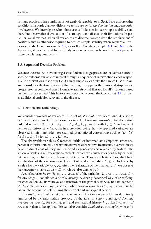
Definition 4.1 We say that the problem exhibits simple stability1 with respect to theinformation base I = (L1, A1, . . . , Ln, An, Y ) if, for each s ∈ S∗, with σ denotingthe non-random regime indicator taking values in {o, s}:

Li ⊥⊥ σ | (Li−1, Ai−1) (i = 1, . . . , n + 1). (9)

Formally, simple stability requires that, for any bounded measurable function f (Li ),there exist a single random variable W = w(Li−1, Ai−1) that serves as a versionof each of the conditional expectations E{ f (Li ) | (Li−1, Ai−1) ; o} and E{ f (Li ) |

1 This definition is slightly weaker than that of Dawid and Didelez [9], as we are only requiring a commonversion of the corresponding conditional expectations between each single control strategy and the obser-vational regime. We do not require that there exist one function that can serve as common version acrossall regimes simultaneously.

123

Stat Biosci

Fig. 1 Stability

A1L1 A2L2 Y

σ

(Li−1, Ai−1) ; s}. This property then extends to conditional expectations of functionsof the form f (Li , Ai−1). In particular, this apparently2 supports identification of theright-hand side of (5) with its observational counterpart, so allowing observationalestimation of this expression.

Simple stability is a very strong assumption, and will be tenable only in veryspecial cases. It will be satisfied if, in the observational regime, the action variablesare physically sequentially randomized: then all unobserved potential confoundingfactors will, on average, be balanced between the treatment groups. Alternatively, wemight accept simple stability if, in the observational regime, the allocation of treatmentis decided taking into account only the domain variables in the information base andnothing more: for example, if we are observing a doctor whose treatment decisions arebased only on the domain variables we are recording, and no additional unrecordedinformation.

An ID describing simple stability (9) for i = 1, 2, 3 is shown in Fig. 1. The specificproperty (9) is represented by the absence of arrows from σ to L1, L2, and L3 ≡ Y .

4.1 Positivity

We have indicated that simple stability might allow us to identify the consequenceof a control strategy s on the basis of data from the observational regime o. How-ever, while this condition ensures the existence of a common version of the relevantconditional expectation, valid for both regimes, deriving this function from the obser-vational regime alone might be problematic, because versions of the same conditionalexpectation can differ on events of probability 0, and we have not ruled out that anevent having probability 0 in one regime might have positive probability in another.Thus we can only obtain the desired function from the observational regime on a setthat has probability 1 in the observational regime; and this might not have probability1 in the interventional regime—see Counter-example A.1 in the Appendix for a simpleexample of this.

To evade this problem, we can impose a condition requiring an event to have zeroprobability in the interventional regime whenever it has zero probability in the obser-vational regime:

2 but see Sect. 4.1 below.

123

Stat Biosci

Definition 4.2 We say the problem exhibits positivity or absolute continuity if, forany interventional regime s ∈ S∗, the joint distribution of (Ln, An, Y ) under Ps isabsolutely continuous with respect to that under Po, i.e.:

Ps(E) > 0 ⇒ Po(E) > 0 (10)

for any event E defined in terms of (Ln, An, Y ).

Suppose we have both simple stability and positivity, and consider a bounded functionh(Li ). Let W = w(Li−1, Ai−1) be any variable that serves both as a version ofE{h(Li ) | Li−1, Ai−1 ; o} and as a version of E{h(Li ) | Li−1, Ai−1 ; s}; such avariable is guaranteed to exist by (9). Let V = v(Li−1, Ai−1) be any version ofE{h(Li ) | Li−1, Ai−1 ; o}. Since W too is a version of E{h(Li ) | Li−1, Ai−1 ; o},V = W, a.s. [Po]. Hence, by (10), V = W, a.s. [Ps]. But since W is a version ofE{h(Li ) | Li−1, Ai−1 ; s}, so too must be V . So we have shown that any version of aconditional expectation calculated under Po will also serve this purpose under Ps . Inparticular, when effecting the G-computation algorithm of Sect. 2.3.1, in (5) we arefully justified in replacing the conditional expectation under Ps by (any version of) itscounterpart under Po—which we can in principle estimate from observational data.

4.1.1 Difficulties with Continuous Actions

When all variables are discrete, positivity will hold if and only if every partial historythat can occur with positive probability in the interventional regime also has a positiveprobability in the observational regime. In particular, this will hold for every interven-tional regime if every possible partial history can occur with positive probability inthe observational regime.

Even in this case we might well need vast quantities of observational data to getgood estimates of all the probabilities needed for substitution into the G-recursionalgorithm—that is the reason for our qualification “in principle” at the end of Sect. 4.1.In practice, even under positivity we would generally need to impose some smoothnessor modelling assumptions to get reasonable estimates of the required observationaldistributions. However we do not explore these issues here, merely noting that, givenenough data to estimate these observational distributions, positivity allows us to trans-fer them to the interventional regime.

When however we are dealing with continuous action variables—as, for example,the dose of a medication—the positivity condition may become totally unreasonable.For a very simple example, consider a single continuous action variable A and responsevariable Y . We might want to transfer the conditional expectation E(Y | A) from theobservational regime o, in which A arises from a continuous distribution, to an inter-ventional regime s, in which it is set to a fixed value, A = a0. However, if we takeany version of E(Y | A; o) and change it, to anything we want, at the single pointA = a0, we will still have a version of E(Y | A; o). So we are unable to identify thedesired E(Y | A; s) This is due to the failure of positivity, since the 1-point interven-tional distribution of A is not absolutely continuous with respect to the continuousobservational distribution of A. Positivity here would require that there be a positive

123

Stat Biosci

probability of observing the exact value a0 in the observational regime. But it wouldnot generally be reasonable to impose such a condition, and quite impossible to do sofor every value a0, that we might be potentially interested in setting for A.

In such a case we might make progress by imposing further structure, such as amodel for E(Y | A; o) that is a continuous function of A, so identifying a preferredversion of this. Here however we shall avoid such problems by only considering prob-lems in which all action variables are discrete. Then we shall have positivity wheneverevery action sequence a having positive interventional probability also has positiveobservational probability, and the (uniquely defined) conditional interventional dis-tribution of all the non-action variables, given A = a, is absolutely continuous withrespect to its observational counterpart. This will typically not be an unreasonablerequirement. We note that this set-up is still more general than usual formulations ofG-recursion, which explicitly or implicitly assume that all variables are discrete.

5 Sequential Ignorability

As we have alluded, simple stability will often not be a compelling assumption, forexample because of the suspected presence of unmeasured confounding variables, andwe might not be willing to accept it without further justification. Here we considerconditions that might seem more acceptable, and investigate when these will, after all,imply simple stability—thus supporting the application of G-recursion.

5.1 Extended Stability and Extended Positivity

Let U denote a set of variables that, while they might potentially influence actionstaken under the observational regime, are not available to the decision maker, and soare not included in his information base I := (L1, A1, . . . , Ln, An, Ln+1 ≡ Y ). Wedefine the extended information base I ′ := (L1, U1, A1, . . . , Ln, Un, An, Ln+1), withUi denoting the variables in U realized just before action Ai is taken. However, whilethus allowing Ui to influence Ai in the observational regime, we still only considerinterventional strategies where there is no such influence—since the decision makerdoes not have access to the (Ui ). This motivates an extended formal definition of“control strategy” in this context:

Definition 5.1 (Control strategy) A regime s is a control strategy if

Ai ⊥⊥ Ui | (Li , Ai−1 ; s) (i = 1, . . . , n) (11)

and in addition, the conditional distribution of Ai , given (Li , Ai−1), under regime s,is known to the analyst.

We again denote the set of interventional regimes corresponding to the control strate-gies under consideration by S∗.

Definition 5.2 We say that the problem exhibits extended stability (with respect tothe extended information base I ′) if, for any s ∈ S∗, with σ denoting the non-randomregime indicator taking values in {o, s}:

123

Stat Biosci

Fig. 2 Extended stability

A1 A2

U1 U2

L2L1

σ

Y

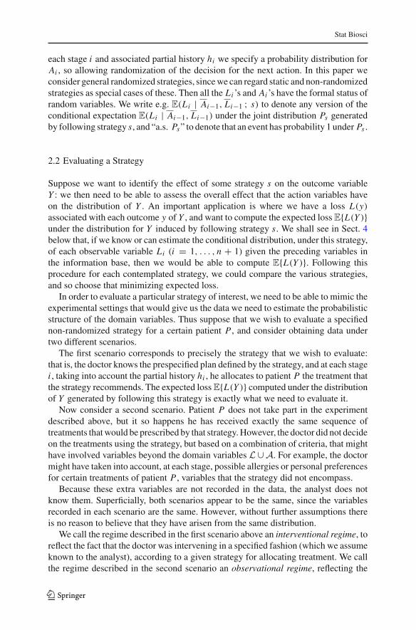
(Li , Ui ) ⊥⊥ σ | (Li−1, Ui−1, Ai−1) (i = 1, . . . , n + 1). (12)

Extended stability is formally the same as simple stability, but using a differentinformation base, where Li is expanded to (Li , Ui ). The real difference is that theextended information base is not available to the decision maker in the interventionalregime, so that his decisions can not take account of the (Ui ). An ID faithfully rep-resenting property (12) for i = 1, 2, 3 is shown in Fig. 23. The property (12) isrepresented by the absence of arrows from σ to L1, U1, L2, U2 and Y . However, thediagram does not explicitly represent the additional property (11), which implies that,when σ = s, the arrows into A1 from U1 and into A2 from U1 and U2 can be dropped.

To evade problems with events of zero probability, we can extend Definition 4.2:

Definition 5.3 We say the problem exhibits extended positivity if, for any s ∈ S∗, thejoint distribution of (U n, Ln, An, Y ) under Ps is absolutely continuous with respectto that under Po, i.e.

Ps(E) > 0 ⇒ Po(E) > 0 (13)

for any event E defined in terms of (Ln, U n, An, Y ).

5.2 Sequential Randomization

Extended stability represents the belief that, for each i , the conditional distribution of(Li , Ui ), given all the earlier variables (Li−1, U i−1, Ai−1) in the extended informationbase, is the same in the observational regime as in the interventional regime. This willtypically be defensible if we can argue that we have included in L∪U all the variablesinfluencing the actions in the observational regime.

However extended stability, while generally more defensible than simple stability,typically does not imply simple stability, which is what is required to support G-

3 Note that the IDs in this paper differ from those in Dawid and Didelez [9].

123

Stat Biosci

Fig. 3 Sequentialrandomization

A1 A2

U1 U2

L2L1

σ

Y

recursion. But it may do so if we impose additional conditions. Here and in Sect. 5.3below we explore two such conditions.

Our first is the following:

Condition 5.3 (Sequential randomization)

Ai ⊥⊥ Ui | (Li , Ai−1 ; o) (i = 1, . . . , n). (14)

Taking account of (11), we see that (14) is equivalent to:

Ai ⊥⊥ Ui | (Li , Ai−1 ; σ) (i = 1, . . . , n) (15)

where σ takes values in S = {o} ∪ S∗.Under sequential randomization, the observational distribution of Ai , given the ear-

lier variables in the information base, would be unaffected by further conditioning onthe earlier unobservable variables, Ui . Hence the (Ui ) are redundant for explaining theway in which actions are determined in the observational regime. While this conditionwill hold under a control strategy, in the observational regime it requires that the onlyinformation that has been used to assign the treatment at each stage is that suppliedby the observable variables. For example, sequential randomization will hold if theactions are physically sequentially randomized within all levels of the earlier variablesin the information base. The following result is therefore unsurprising.

Theorem 5.1 Suppose we have both extended stability, (12) and sequential random-ization, (15). Then we have simple stability, (9).

An ID faithfully representing the conditional independence relationships assumed inTheorem 5.1, for i = 1, 2, 3, is shown in Fig. 3. Figure 3 can be obtained from Fig. 2on deleting the arrows into A1 from U1 and into A2 from U1 and U2, so representing(15). (However, as we shall see below in Sect. 5.3, in general such “surgery” on IDscan be hazardous.)

The conditional independence properties (9) characterizing simple stability cannow be read off from Fig. 3, by applying the d-separation or moralization criteria.

123

Stat Biosci

Fig. 4 Sequential irrelevance?

A1 A2

U1 U2

L2L1

σ

Y

For a formal algebraic proof of Theorem 5.1, using just the axioms of conditionalindependence as given in Theorem 3.1, see Theorem 6.1 of Dawid and Didelez [9]4.

Corollary 5.1 Suppose we have extended stability, sequential randomization, andsimple positivity. Then we can apply G-recursion to compute the consequence of astrategy s ∈ S∗.

5.3 Sequential Irrelevance

Consider now the following alternative condition:

Condition 5.4 (Sequential Irrelevance)

Li ⊥⊥ Ui−1 | (Li−1, Ai−1 ; σ) (i = 1, . . . , n + 1). (16)

Under sequential irrelevance, in both regimes the conditional distribution of theobservable variable(s) at stage i is unaffected by the history of unobservable variablesup to the previous stage i − 1, given the domain variables in the information baseup to the previous stage. In contrast to (15), (16) permits the unobserved variablesthat appear in earlier stages to influence the next action Ai (which can only happenin the observational regime)—but not the development of the subsequent observablevariables (including the ultimate response variable Y ). This will hold when at eachstage i the unobserved variable Ui does not affect the development of future L’s: forexample, Ui might represent the inclination of the patient to take the current treatmentAi . In general, the validity of this assumption will have to be justified in the contextof the problem under study.

By analogy with the passage from Figs. 2 to 3, we might attempt to represent theadditional assumption (16) by removing from Fig. 2 all arrows from U j to Li ( j < i).This would yield Fig. 4. On applying d-separation or moralization to Fig. 4 we could

4 Note that, in either of these approaches, we can restrict σ to the two values o and s, so fully justifyingtreating the non-stochastic variable σ as if it were stochastic.

123

Stat Biosci

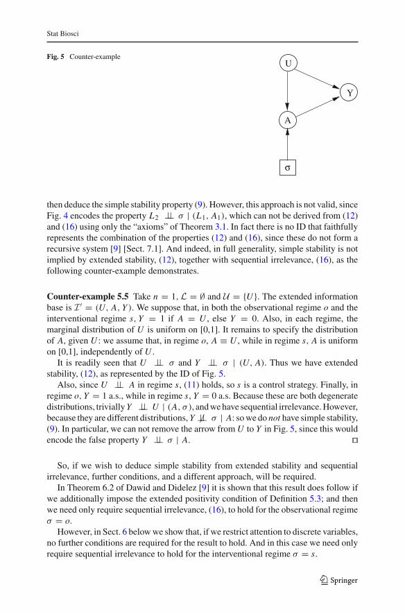
Fig. 5 Counter-example

A

σ

Y

U

then deduce the simple stability property (9). However, this approach is not valid, sinceFig. 4 encodes the property L2 ⊥⊥ σ | (L1, A1), which can not be derived from (12)and (16) using only the “axioms” of Theorem 3.1. In fact there is no ID that faithfullyrepresents the combination of the properties (12) and (16), since these do not form arecursive system [9] [Sect. 7.1]. And indeed, in full generality, simple stability is notimplied by extended stability, (12), together with sequential irrelevance, (16), as thefollowing counter-example demonstrates.

Counter-example 5.5 Take n = 1,L = ∅ and U = {U }. The extended informationbase is I ′ = (U, A, Y ). We suppose that, in both the observational regime o and theinterventional regime s, Y = 1 if A = U , else Y = 0. Also, in each regime, themarginal distribution of U is uniform on [0,1]. It remains to specify the distributionof A, given U : we assume that, in regime o, A ≡ U , while in regime s, A is uniformon [0,1], independently of U .

It is readily seen that U ⊥⊥ σ and Y ⊥⊥ σ | (U, A). Thus we have extendedstability, (12), as represented by the ID of Fig. 5.

Also, since U ⊥⊥ A in regime s, (11) holds, so s is a control strategy. Finally, inregime o, Y = 1 a.s., while in regime s, Y = 0 a.s. Because these are both degeneratedistributions, trivially Y ⊥⊥ U | (A, σ ), and we have sequential irrelevance. However,because they are different distributions, Y �⊥⊥ σ | A: so we do not have simple stability,(9). In particular, we can not remove the arrow from U to Y in Fig. 5, since this wouldencode the false property Y ⊥⊥ σ | A. ��

So, if we wish to deduce simple stability from extended stability and sequentialirrelevance, further conditions, and a different approach, will be required.

In Theorem 6.2 of Dawid and Didelez [9] it is shown that this result does follow ifwe additionally impose the extended positivity condition of Definition 5.3; and thenwe need only require sequential irrelevance, (16), to hold for the observational regimeσ = o.

However, in Sect. 6 below we show that, if we restrict attention to discrete variables,no further conditions are required for the result to hold. And in this case we need onlyrequire sequential irrelevance to hold for the interventional regime σ = s.

123

Stat Biosci

6 Discrete Case

In this section we assume all variables are discrete, and denote P(A = a, L = l) byp(a, l), etc.

To control null events, we need the following lemma:

Lemma 6.1 Let all variables be discrete. Suppose that we have extended stability,(12), and let s be a control strategy, so that (11) holds. Then, for any (uk, lk, ak) suchthat

Ak: p(lk, ak ; s) > 0, andBk: p(uk, lk, ak ; o) > 0, we haveCk: p(uk, lk, ak ; s) > 0.

Proof Let Hk denote the assertion that Ak and Bk imply Ck. We establish Hk byinduction.

To start, we note that H0 holds vacuously.Now suppose Hk−1 holds. Assume further Ak and Bk. Together these conditions

imply that all terms appearing throughout the following argument are positive.We have

p(uk, lk, ak ; s) = p(uk | lk, ak ; s) p(lk, ak ; s)

= p(uk | lk, ak−1 ; s) p(lk, ak ; s) (17)

= p(uk, lk, ak−1 ; s)

p(lk, ak−1 ; s)p(lk, ak ; s)

= p(uk, lk | uk−1, lk−1, ak−1 ; s)

× p(uk−1, lk−1, ak−1 ; s) p(lk, ak ; s)

p(lk, ak−1 ; s)

= p(uk, lk | uk−1, lk−1, ak−1 ; o)

× p(uk−1, lk−1, ak−1 ; s) p(lk, ak ; s)

p(lk, ak−1 ; s)(18)

= p(uk, lk, ak−1 ; o)

p(uk−1, lk−1, ak−1 ; o)

× p(uk−1, lk−1, ak−1 ; s) p(lk, ak ; s)

p(lk, ak−1 ; s)> 0.

Here (17) holds by (11) and (18) holds by (12). The induction is established. ��Theorem 6.1 Suppose the conditions of Lemma 6.1 apply, and, further, that we havesequential irrelevance in the interventional regime s:

Li ⊥⊥ Ui−1 | (Li−1, Ai−1 ; s) (i = 1, . . . , n + 1). (19)

123

Stat Biosci

Then the simple stability property (9) holds.

Proof The result will be established if we can show that, for any li , we can find afunction w(Li−1, Ai−1) such that, for both σ = o and σ = s,

p(li | li−1, ai−1 ; σ) = w(li−1, ai−1)

whenever p(li−1, ai−1 ; σ) > 0.This is trivially possible if either regime gives probability 0 to (li−1, ai−1). So

suppose p(li−1, ai−1 ; σ) > 0 for both regimes. Then

p(li | li−1, ai−1 ; o) =∑ui−1

′p(li | ui−1, li−1, ai−1 ; o) × p(ui−1 | li−1, ai−1 ; o)

(20)

where∑′ denotes summation restricted to terms for which p(ui−1, li−1, ai−1 ; o) >

0—and so, by Lemma 6.1, p(ui−1, li−1, ai−1 ; s) > 0. Then by (12),

p(li | li−1, ai−1 ; o) =∑ui−1

′p(li | ui−1, li−1, ai−1 ; s) × p(ui−1 | li−1, ai−1 ; o)

=∑ui−1

′p(li | li−1, ai−1 ; s) × p(ui−1 | li−1, ai−1 ; o) (21)

= p(li | li−1, ai−1 ; s)

where (21) holds by (19). Thus we can take

w(li−1, ai−1) := p(li | li−1, ai−1 ; s)

to conclude the proof. ��Counter-example A.2 in the Appendix demonstrates that, even in this discrete case,

to deduce simple stability under the conditions of Lemma 6.1 it is not sufficient toimpose sequential irrelevance only for the observational regime o.

We summarise our findings on sequential irrelevance in the following corollary:

Corollary 6.1 Suppose we have extended stability, sequential irrelevance, andextended positivity. Then we can apply G-recursion to compute the consequence of astrategy s ∈ S∗. In the special case that all variables in the extended information baseare discrete, we can replace the condition of extended positivity by simple positivity.

7 Conclusion

The decision-theoretic approach to causal inference focuses on the possibilities fortransferring probabilistic information between different stochastic regimes. In this

123

Stat Biosci

paper we have developed a formal underpinning for this approach, based on an exten-sion of the axiomatic theory of conditional independence to include non-stochasticvariables. This formal foundation now supplies a rigorous justification for variousmore informal arguments that have previously been presented [3,8,9].

By applying this theory to the problem of dynamic treatment assignment, we haveshown how, and under what additional conditions, the assumptions of sequential ran-domization or sequential irrelevance can support observational identification of theconsequence of some treatment strategy under consideration. Specifically, in orderto identify the consequence of a control strategy directly from observational data bymeans of G-recursion, we should like to establish the properties of simple positivityand simple stability. Simple positivity will often be a reasonable assumption to imposedirectly, at any rate when all the action variables are discrete. However, simple stabilitymay be harder to justify. Instead, we might begin with the weaker and more readily jus-tifiable assumption of extended stability. We have investigated when, in combinationwith appropriate additional conditions, extended stability will imply simple stability.

Our first additional condition is sequential randomization. Extended stability andsequential randomization together imply simple stability, even without imposing anypositivity assumption. (However, for the purposes of complete identification of a con-trol strategy from observational data using G-recursion, we still need to require simplepositivity, in order to guarantee that any version of the desired conditional expectationthat can be recovered from the observational regime can simultaneously serve as aversion for the interventional regime.)

The second condition studied is sequential irrelevance. However, extended stabilitytogether with sequential irrelevance are not in general sufficient to imply simple sta-bility, and a further assumption of extended positivity is typically also needed. Sinceextended positivity implies simple positivity, these conditions are jointly sufficient toenable identification of a control strategy from observational data using G-recursion.However, since the property of extended positivity involves unobservable variables,justifying this assumption can be problematic. We have shown that, in the special casethat all the random variables involved are discrete, we can dispense with this additionalassumption. (Of course, we will still need the weaker assumption of simple positivityto support G-recursion.) In the presence of continuous random variables, we haveshown, by means of a counterexample, that the assumption of extended positivity maybe indispensible.

In the light of our analysis, we offer the following advice to the analyst who wishesto use observational data in order to evaluate a control strategy: Examine carefullywhich of the assumptions enabling application of G-recursion can be sensibly justifiedin the context of the problem under study. In particular, can simple stability reasonablybe assumed? — since otherwise (as we discussed in Sect. 2.2) a naïve analysis maysuffer from bias.

Whereas for data obtained from a randomized control trial the assumption of simplestability may be robustly defensible, for more typical observational regimes the analystwould need to be able to present a good argument for assuming simple stability. Ourconditions of sequential randomization and sequential irrelevance, together with theadditional supporting conditions we have identified, supply a possible route to makingsuch an argument.

123

Stat Biosci

Appendix: The Need for Positivity

Counter-example A.1 The following counter-example illustrates what can go wrongwhen we do not have positivity: even when a property such as (7) holds, we can notuse just any version of the conditional expectation in one regime to serve as a versionof this conditional expectation in another regime.

Consider a sequential decision problem of n = 2 stages with domain variablesL1, A and L2, where A is a binary variable with A = 0 denoting no treatment andA = 1 denoting treatment. In the observational regime o, the treatment is never given:Po(A = 0) = 1; while in the interventional regime s, the treatment is always given:Ps(A = 1) = 1. We thus have failure of the positivity requirement of Definition 4.2.

Suppose that,in both regimes, L1 = 0 or 1 each with probability 1/2, and L2 =L1 + A. Then, with σ denoting the regime indicator taking values in S = {o, s}, wetrivially have L2 ⊥⊥ σ | (L1, A).

Now consider the variables

Wo ={

L1 if A = 00 if A = 1

and

Ws ={

2 if A = 0L1 + 1 if A = 1.

Then Wo = L2 a.s. [Po], so Wo serves as a version of E(L2 | L1, A ; o); alsoWs = L2 a.s. [Ps], so Ws serves as a version of E(L2 | L1, A ; s). However, almostsurely under both Po and Ps , Wo �= Ws , and neither of these variables supplies aversion of E(L2 | L1, A) simultaneously valid in both regimes. ��

Counter-example A.2 In Sect. 6 we have seen that, when all random variables arediscrete and the conditions of Lemma 6.1 are satisfied, in order to be able to deducesimple stability it is sufficient to require sequential irrelevance only for the interven-tional regime. However, without the positivity assumption simple stability does not

Table 1 Sequential irrelevancein the observational regime

σ = o σ = s

P(U1 = 0, A1 = 0, Y = 0) 0 98

P(U1 = 0, A1 = 0, Y = 1) 0 77

P(U1 = 0, A1 = 1, Y = 0) 315 252

P(U1 = 0, A1 = 1, Y = 1) 560 448

P(U1 = 1, A1 = 0, Y = 0) 50 25

P(U1 = 1, A1 = 0, Y = 1) 200 100

P(U1 = 1, A1 = 1, Y = 0) 135 180

P(U1 = 1, A1 = 1, Y = 1) 240 320

123

Stat Biosci

follow if, additionally to the requirements of Lemma 6.1, we instead require sequentialirrelevance only for the observational regime.

Consider a sequential decision problem of n = 2 stages with extended infor-mation base I ′ := (U1, A1, L2 = Y ); L1 and U2 are trivial and so absent.The joint distribution of the variables in I ′ in the two regimes σ = o or s issupposed given by Table 1, where the probabilities are to be taken over 1500(

e.g.P(U1 = 0, A1 = 1, Y = 0 ; s) = 2521500

).

The reader may check that extended stability, (12), holds, and that s is a controlstrategy: (11) holds. Also, sequential irrelevance, (16), holds for the observationalregime, though not the interventional regime. But simple stability, (9), does not hold.

��Acknowledgments PC acknowledges funding by the Engineering and Physical Sciences Research Coun-cil (EPSRC).

Open Access This article is distributed under the terms of the Creative Commons Attribution Licensewhich permits any use, distribution, and reproduction in any medium, provided the original author(s) andthe source are credited.

References

1. Constantinou P (2013) Conditional independence and applications in statistical causality. Ph.D. Dis-sertation, University of Cambridge

2. Cowell RG, Dawid AP, Lauritzen SL, Spiegelhalter DJ (2007) Probabilistic networks and expertsystems: exact computational methods for Bayesian networks. Springer, New York

3. Dawid AP (1979) Conditional independence in statistical theory. J R Stat Soc Ser B 41(1):1–314. Dawid AP (1979) Some misleading arguments involving conditional independence. J R Stat Soc Ser

B 41(2):249–2525. Dawid AP (1980) Conditional independence for statistical operations. Ann Stat 8(3):598–6176. Dawid AP (1998) Conditional independence. In: Kotz S, Read CB, Banks DL (eds) Encyclopedia of

statistical sciences, update vol 2. Wiley, New York, pp 146–155. doi:10.1002/0471667196.ess0618.pub2

7. Dawid AP (2001) Separoids: a mathematical framework for conditional independence and irrelevance.Ann Math Artif Intell 32:335–372. doi:10.1023/A:1016734104787

8. Dawid AP (2002) Influence diagrams for causal modelling and inference. Int Stat Rev 70(2):161–189.doi:10.1111/j.1751-5823.2002.tb00354.x

9. Dawid AP, Didelez V (2010) Identifying the consequences of dynamic treatment strategies: a decision-theoretic overview. Stat Surv 4:184–231. doi:10.1214/10-SS081

10. Lauritzen SL, Dawid AP, Larsen BN, Leimer HG (1990) Independence properties of directed Markovfields. Networks 20(5):491–505. doi:10.1002/net.3230200503

11. Murphy SA (2003) Optimal dynamic treatment regimes. J R Stat Soc Ser B 65:331–355. doi:10.1111/1467-9868.00389

12. Pearl J (1988) Probabilistic reasoning in intelligent systems: networks of plausible inference. MorganKaufmann Publishers Inc., San Francisco

13. Robins J (1986) A new approach to causal inference in mortality studies with a sustained exposureperiod–application to control of the healthy worker survivor effect. Math Model 7:1393–1512. doi:10.1016/0270-0255(86)90088-6

14. Robins J (1987) Addendum to “A new approach to causal inference in mortality studies with sustainedexposure periods–application to control of the healthy worker survivor effect”. Comput Math Appl14:923–945

15. Robins J (1989) The analysis of randomized and nonrandomized AIDS treatment trials using a newapproach to causal inference in longitudinal studies. In: L Sechrest HF, Mulley A (eds) Health serviceresearch methodology: a focus on AIDS, NCSHR, U.S. Public Health Service, pp 113–159

123

Stat Biosci

16. Robins J (1992) Estimation of the time-dependent accelerated failure time model in the presence ofconfounding factors. Biometrika 79:321–324

17. Robins J (1997) Causal inference from complex longitudinal data. In: Berkane M (ed) Latent variablemodeling and applications to causality. Lecture Notes in Statistics, vol 120. Springer, New York, pp69–117

18. Rosthøj S, Fullwood C, Henderson R, Stewart S (2006) Estimation of optimal dynamic anticoagulationregimes from observational data: a regret-based approach. Stat Med 25(24):4197–4215. doi:10.1002/sim.2694

19. Sterne JAC, May M, Costagliola D, de Wolf F, Phillips AN, Harris R, Funk MJ, Geskus RB, GillJ, Dabis F, Miro JM, Justice AC, Ledergerber B, Fatkenheuer G, Hogg RS, D’Arminio-MonforteA, Saag M, Smith C, Staszewski S, Egger M, Cole SR (2009) Timing of initiation of antiretroviraltherapy in AIDS-free HIV-1-infected patients: a collaborative analysis of 18 HIV cohort studies. Lancet373:1352–1363. doi:10.1016/S0140-6736(09)60612-7

123