A Forecasting system for the Southern California Current

Emanuele Di LorenzoArthur Miller

Bruce Cornuelle

Scripps Institution of Oceanography, UCSD

Forecast the mesoscale eddies

Understand the physics that control their generation and evolution

Assess the biological response

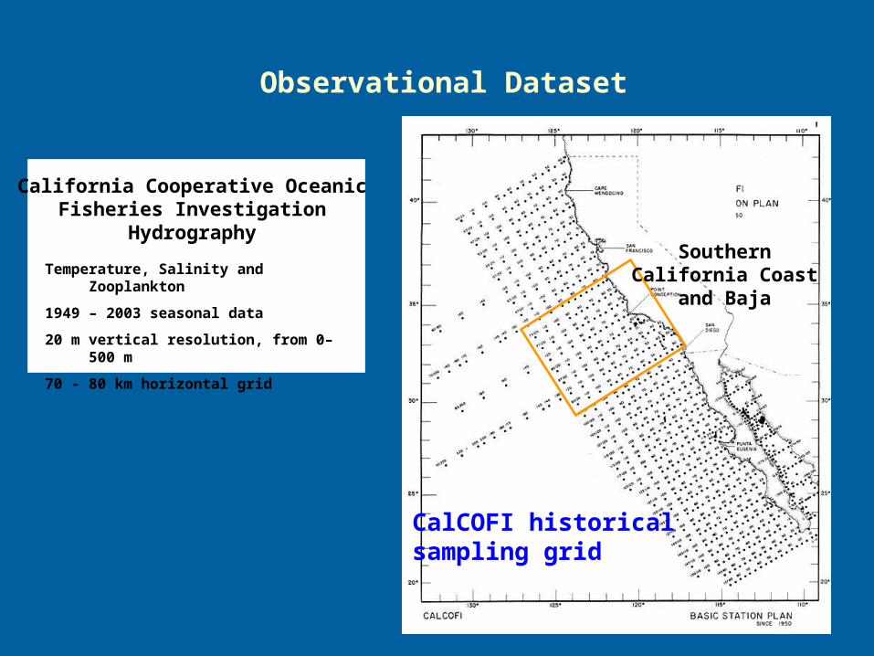
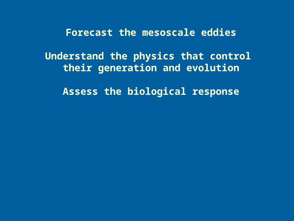
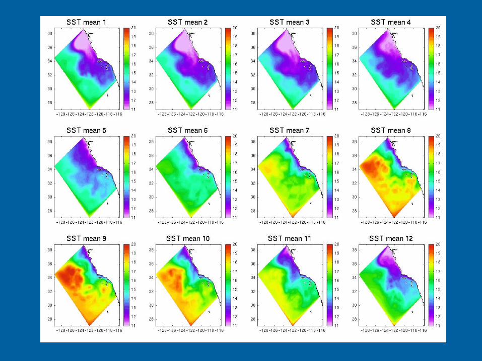
Observational Dataset

SouthernCalifornia Coast

and Baja

Temperature, Salinity and Zooplankton

1949 – 2003 seasonal data

20 m vertical resolution, from 0– 500 m

70 - 80 km horizontal grid

CalCOFI historicalsampling grid

California Cooperative OceanicFisheries Investigation

Hydrography

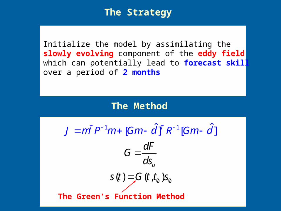
The Strategy

Initialize the model by assimilating the slowly evolving component of the eddy fieldwhich can potentially lead to forecast skill over a period of 2 months

The Strategy

The Method

1

0 0

1ˆ ˆ

( ) (

[ ]

, )

[ ]

o

T T

dFG

ds

s t

J m P m Gm

G

d R

t

G

t

m d

s

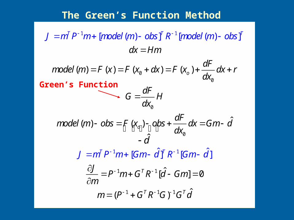
The Green’s Function Method

Initialize the model by assimilating the slowly evolving component of the eddy fieldwhich can potentially lead to forecast skill over a period of 2 months

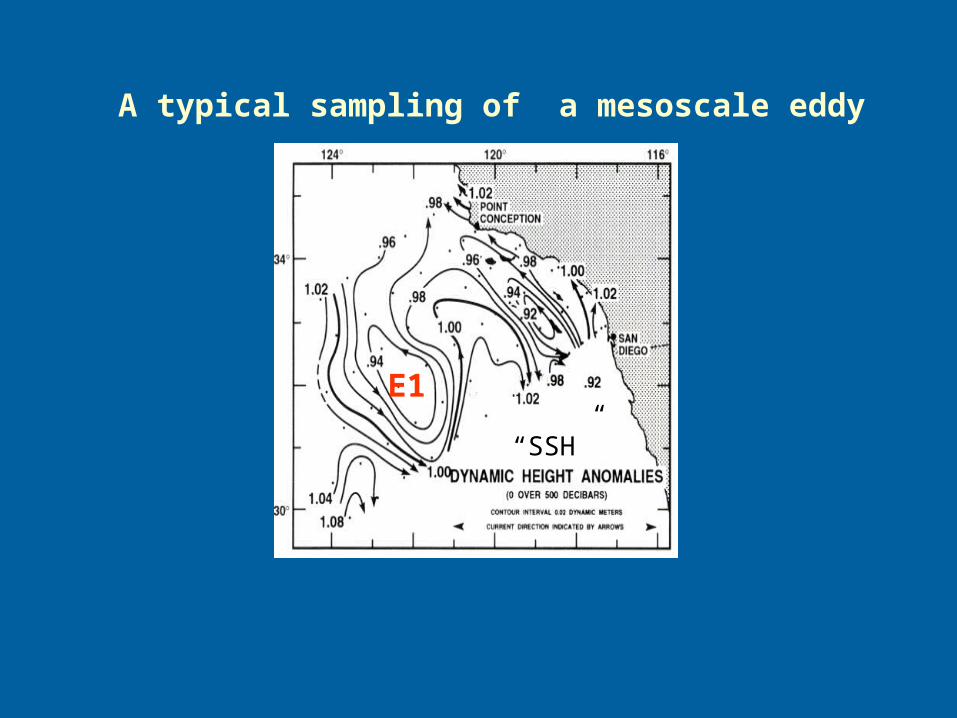
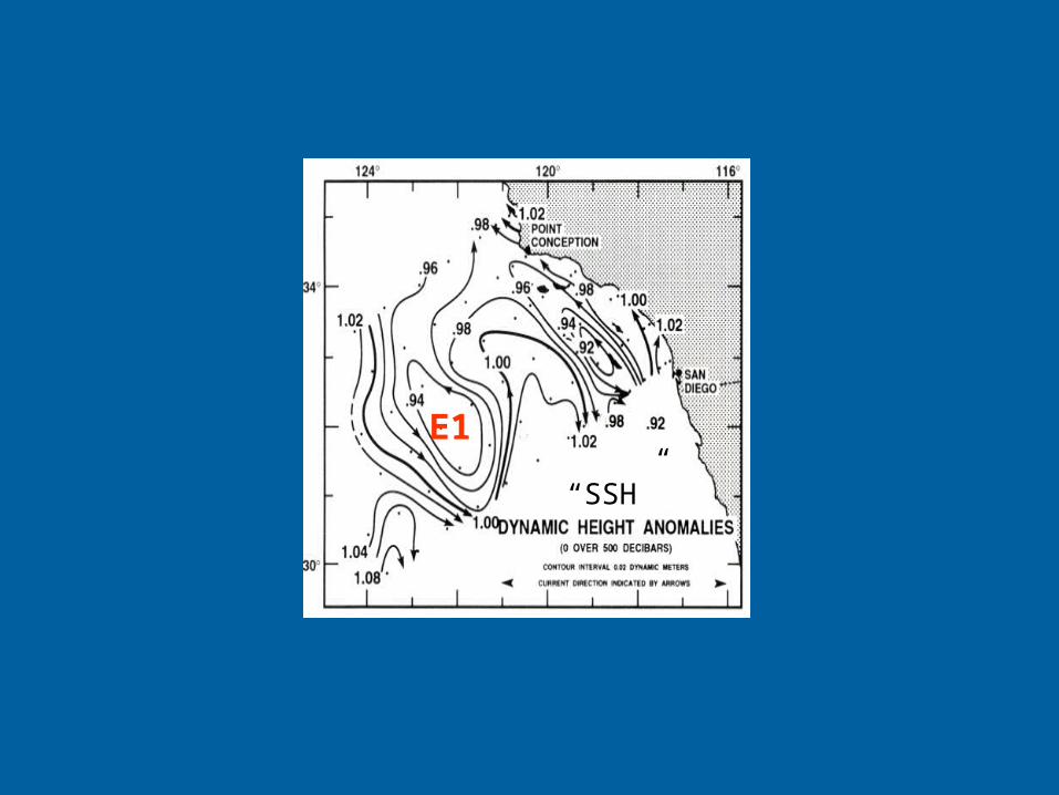
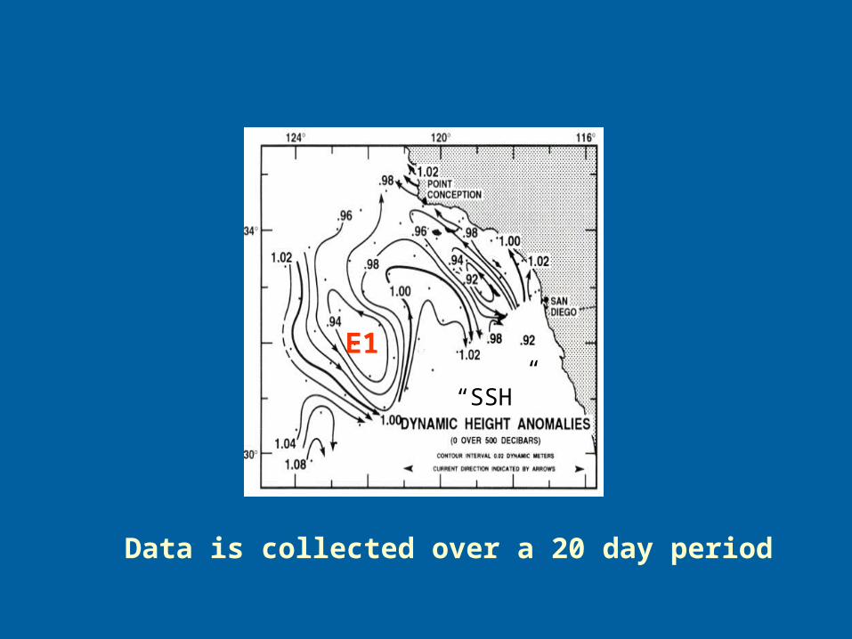
A typical sampling of a mesoscale eddy

E1

“SSH”

AVVISO TOPEX/ERS

[m]

E1

E2SSH

E1

E2

E1

“SSH”

SSH

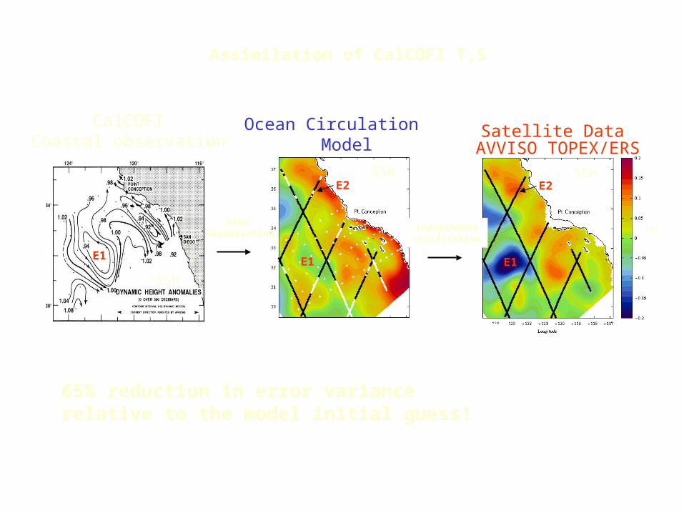
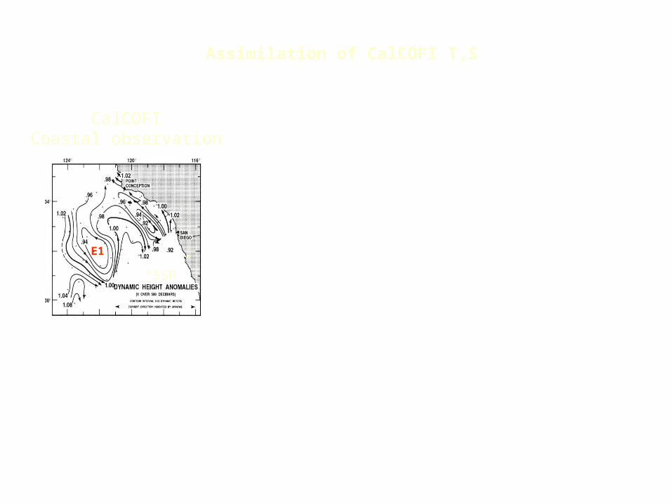
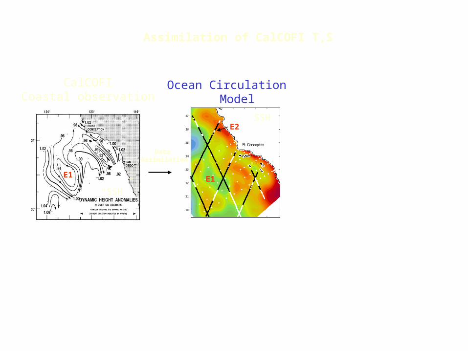
CalCOFICoastal observation

Data Assimilation

Ocean CirculationModel

Satellite Data

Independentverification

Assimilation of CalCOFI T,S

65% reduction in error variancerelative to the model initial guess!

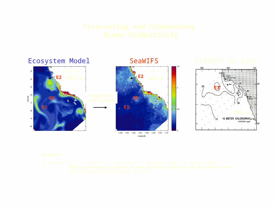
SeaWIFS [M N/m3]

E2

E1

E3

Chl-a

[M N/m3]

E1

E2

E3

Chl-a

E3

Chl-a

Ecosystem Model

Forecasting and Hindcasting Ocean Productivity

Independentverification

CalCOFI in Situ

REFERENCE:

Di Lorenzo, E., A. J. Miller, D. J. Neilson, B. D. Cornuelle, and J. R. Moisan, 2003: Modeling observed California Current mesoscale eddies and the ecosystem response. International Journal of Remote Sensing, in press.

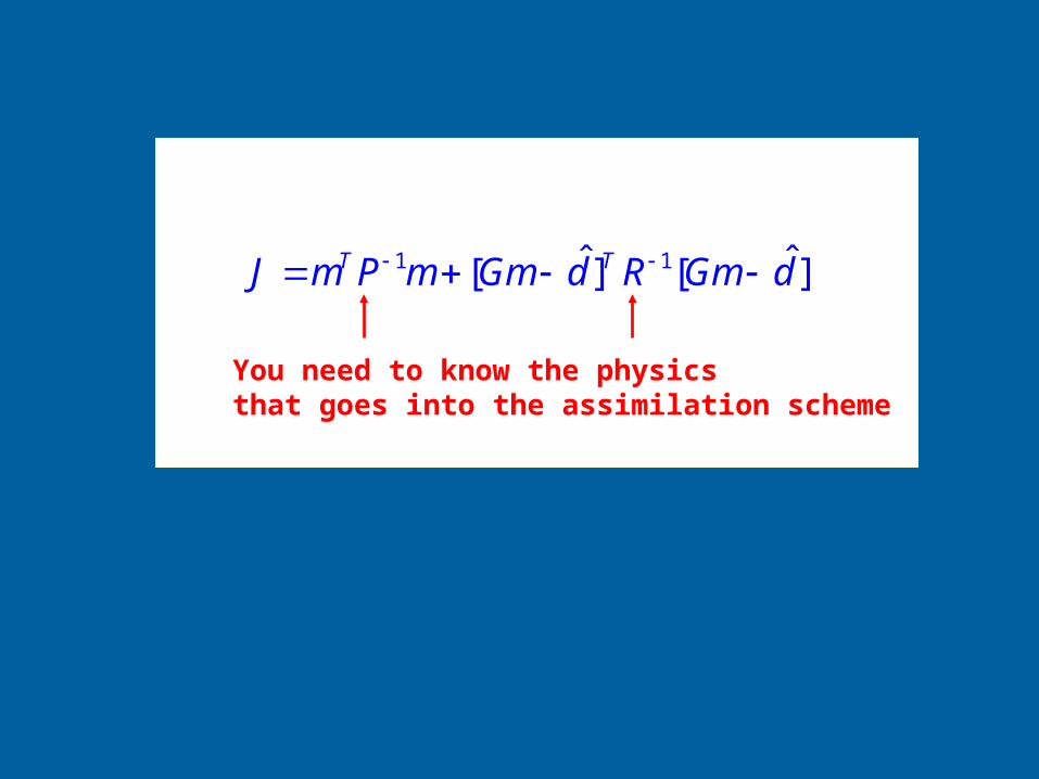
1 1ˆ ˆ[ ] [ ]T TJ m P m Gm d R Gm d

You need to know the physics that goes into the assimilation scheme

E1

“SSH”

1

0JAN APR JUL OCT JAN APR JUL OCT JAN APR JUL OCT

30

60

40

50

10

20

30

60

40

50

10

20

30

60

40

50

10

20

0.5

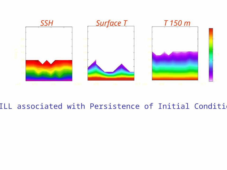
SKILL associated with Persistence of Initial Condition

SSH Surface T T 150 mda

ys

E1

“SSH”

Data is collected over a 20 day period

JAN APR JUL OCT

1

0JAN APR JUL OCT JAN APR JUL OCT

30

60

40

50

10

20

30

60

40

50

10

20

30

60

40

50

10

20

0.5

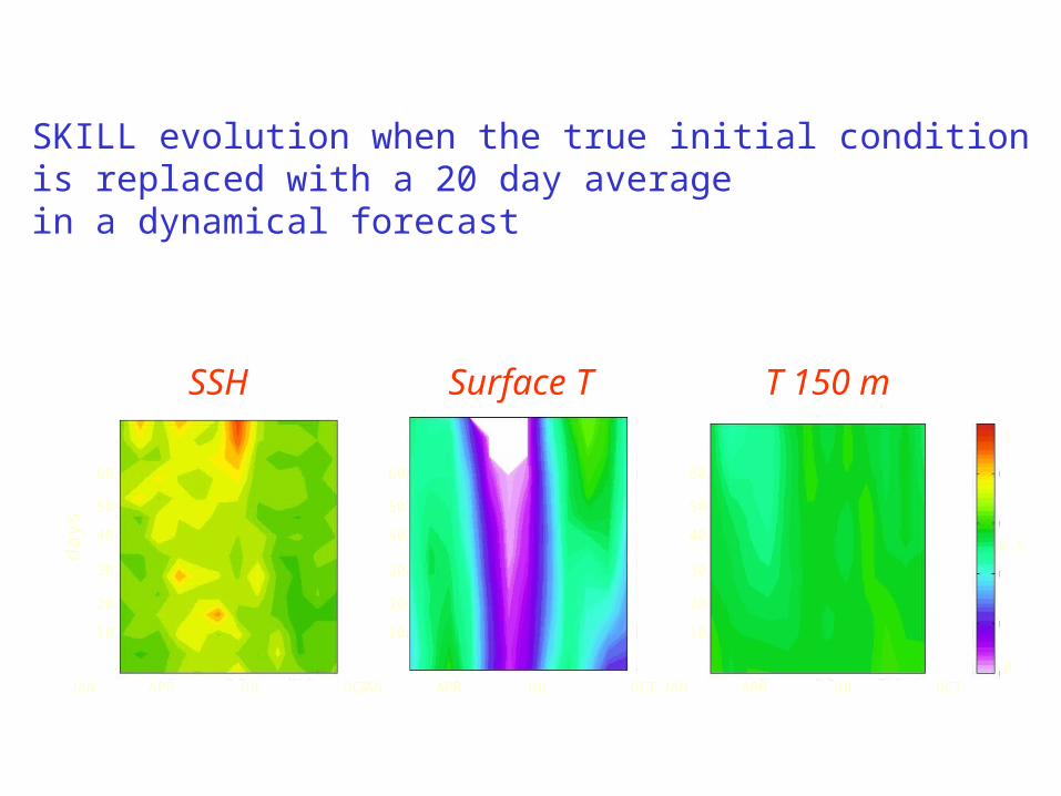
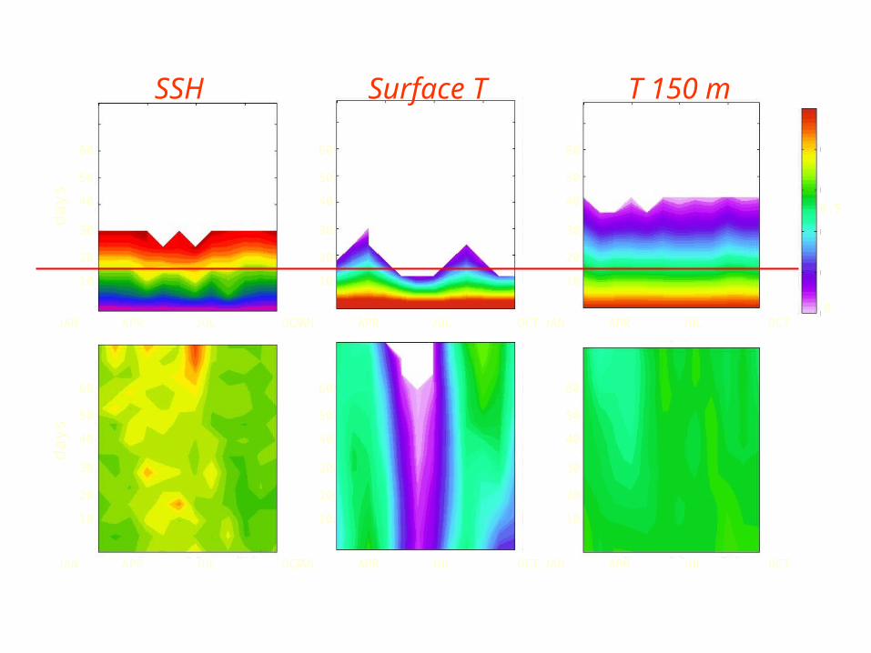
SSH Surface T T 150 m

days

SKILL evolution when the true initial condition is replaced with a 20 day averagein a dynamical forecast

JAN APR JUL OCT

1

0

JAN APR JUL OCT

JAN APR JUL OCT JAN APR JUL OCT JAN APR JUL OCT

JAN APR JUL OCT

30

60

40

50

10

20

30

60

40

50

10

20

30

60

40

50

10

20

30

60

40

50

10

20

30

60

40

50

10

20

30

60

40

50

10

20

0.5

SSH Surface T T 150 mda

ysda

ys

How about the uncertainties in Forcing Functions?

1

0JAN APR JUL OCT JAN APR JUL OCT

30

60

40

50

10

20

30

60

40

50

10

20

0.5

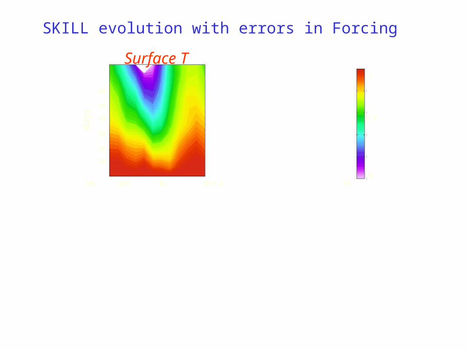
SKILL evolution with errors in Forcing

Surface T T 150 m

days

JAN APR JUL OCT

1

0JAN APR JUL OCT JAN APR JUL OCT

JAN APR JUL OCT

30

60

40

50

10

20

30

60

40

50

10

20

30

60

40

50

10

20

30

60

40

50

10

20

0.5

SKILL evolution with errors in Forcing (and Open BC)

Surface T T 150 m

days

days

SKILL evolution with errors in initial conditionJUNE

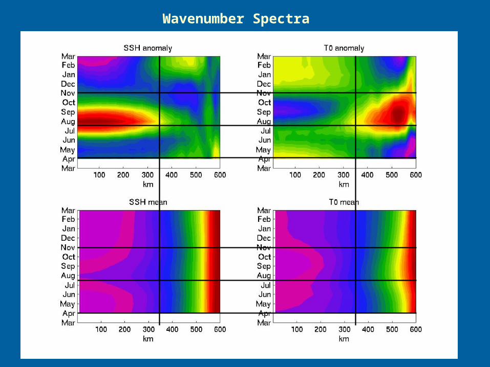
Wavenumber Spectra

Forecast the mesoscale eddies

Real time forecast of CalCOFI in April 2003SCCOOS nowcast-forecast with UCLA and JPL

Understand the physics that control their generation and evolution

Error CovariancesSeasonal dependence

Assess the biological response

In progress….

Concluding remarks:

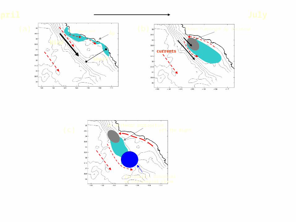
ΔρEkman Pumping Δρ increase

Δh westward propagation off the Bight

Wind

P. Conception

Shelf

(a)

Instability processeson continental slope

currents

(b)

(c)

April July

Ocean Temperature

ZooplanktonLoge Tot. Vol.

5

7

6

4

Anomalies

199019701950 200019801960

C

-1

1

0

Observationsalong the California Coast

Assimilation Method

E1

“SSH”

CalCOFICoastal observation

Assimilation of CalCOFI T,S

E1

E2

E1

“SSH”

SSH

CalCOFICoastal observation

Data Assimilation

Ocean CirculationModel

Assimilation of CalCOFI T,S

What have we learned about the mesoscale dynamics?

What have we learned about the mesoscale dynamics?

00

0

0

1 1

1

1 1

1 1

1

( ) ( ) ( ) ( )

ˆ( )

[ ( ) ] [ ( ) ]

( )

ˆ[ ] 0

(

ˆ ˆ[ ] [ ]

ˆ

o

o

T

T

T T T

T T

J m P m m

dx Hm

dFmodel m F x F x dx F x dx r

dx

dFG H

dx

dFmodel m obs F x obs dx Gm d

dx

JP m G R d Gm

m

m P

odel m obs R model m obs

J m P m Gm d R G

R

m d

G

d

1 ˆ) TG G d

The Green’s Function Method

Green’s Function

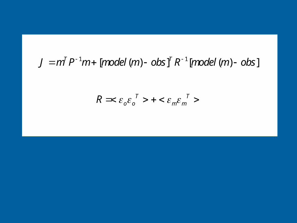
1 1[ ( ) ] [ ( ) ]T TJ m P m model m obs R model m obs

T To o m mR

JAN APR JUL OCT

1

0JAN APR JUL OCT JAN APR JUL OCT

JAN APR JUL OCT

30

60

40

50

10

20

30

60

40

50

10

20

30

60

40

50

10

20

30

60

40

50

10

20

0.5

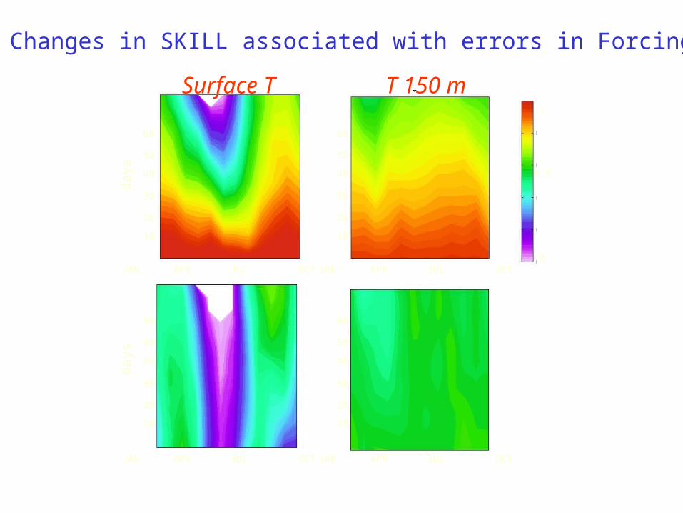
Changes in SKILL associated with errors in Forcing

Surface T T 150 m

days

days