Embed Size (px)
Citation preview

A Flexible New Technique A Flexible New Technique for Camera Calibrationfor Camera CalibrationZhengyou ZhangZhengyou Zhang
Sung HuhCSPS 643 Individual Presentation 1February 25, 2009
1

OutlineOutlineIntroductionEquations and ConstraintsCalibration and ProcedureExperimental ResultsConclusion
2
OutlineOutlineIntroductionEquations and ConstraintsCalibration and ProcedureExperimental ResultsConclusion
3

IntroductionIntroductionExtract metric information from
2D imagesMuch work has been done by
photogrammetry and computer vision community◦Photogrammetric calibration◦Self-calibration
4
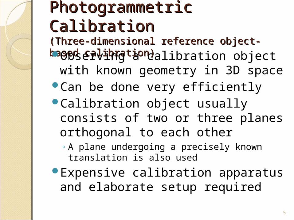
Photogrammetric CalibrationPhotogrammetric Calibration(Three-dimensional reference object-based (Three-dimensional reference object-based calibration)calibration)Observing a calibration object
with known geometry in 3D spaceCan be done very efficientlyCalibration object usually consists
of two or three planes orthogonal to each other◦ A plane undergoing a precisely known
translation is also used
Expensive calibration apparatus and elaborate setup required
5
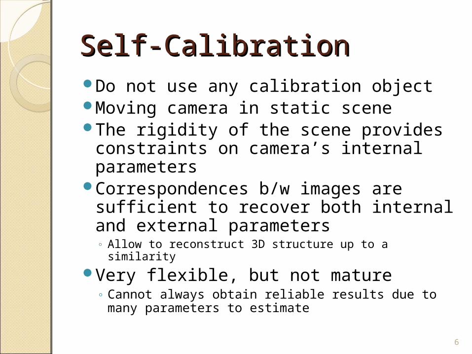
Self-CalibrationSelf-CalibrationDo not use any calibration objectMoving camera in static sceneThe rigidity of the scene provides
constraints on camera’s internal parameters
Correspondences b/w images are sufficient to recover both internal and external parameters◦ Allow to reconstruct 3D structure up to a similarity
Very flexible, but not mature◦ Cannot always obtain reliable results due to
many parameters to estimate
6

Other TechniquesOther TechniquesVanishing points for orthogonal
directionsCalibration from pure rotation
7

New Technique from New Technique from AuthorAuthorFocused on a desktop vision system
(DVS)Considered flexibility, robustness,
and low costOnly require the camera to observe
a planar pattern shown at a few (minimum 2) different orientations◦ Pattern can be printed and attached on planer surface◦ Either camera or planar pattern can be moved by hand
More flexible and robust than traditional techniques◦ Easy setup◦ Anyone can make calibration pattern
8

OutlineOutlineIntroductionEquations and ConstraintsCalibration and ProcedureExperimental ResultsConclusion
9

NotationNotation2D point,3D point,Augmented Vector,Relationship b/w 3D point M and
image projection m
,T
u vm
, ,T
X Y ZM
, ,1 , , , ,1T T
u v X Y Z m M
s m A R t M0
00
0 0 1
u
v
A
10
(1)

NotationNotations: extrinsic parameters that relates
the world coord. system to the camera coord. System
A: Camera intrinsic matrix(u0,v0): coordinates of the principal
pointα,β: scale factors in image u and v
axesγ: parameter describing the skew of
the two image11

Homography b/w the Model Homography b/w the Model Plane and Its ImagePlane and Its ImageAssume the model plane is on Z = 0Denote ith column of the rotation
matrix R by ri
Relation b/w model point M and image m
H is homography and defined up to a scale factor
1 2 3 1 201 1
1
Xu X
Ys v Y
A r r r t A r r t
s m HM 1 2H A r r t
12
(2)
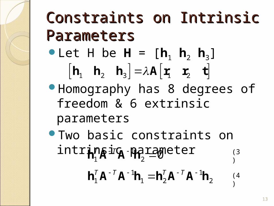
Constraints on Intrinsic Constraints on Intrinsic ParametersParametersLet H be H = [h1 h2 h3]
Homography has 8 degrees of freedom & 6 extrinsic parameters
Two basic constraints on intrinsic parameter
1 2 3 1 2h h h A r r t
11 2 0T T h A A h
1 11 1 2 2T T T T h A A h h A A h
13
(3)
(4)

Geometric InterpretationGeometric InterpretationModel plane described in camera
coordinate system
Model plane intersects the plane at infinity at a line
3
3
00,
1
T
T
x
y w
z w
w
r
r t
1 2,0 0
r r
14

Geometric InterpretationGeometric Interpretation
x∞ is circular point and satisfy , or
a2 + b2 = 0Two intersection points
This point is invariant to Euclidean transformation
1 2
0 0a b
r rx
0T x x
1 2
0
ia
r rx
15

Geometric InterpretationGeometric InterpretationProjection of x∞ in the image plane
Point is on the image of the absolute conic, described by A-TA-1
Setting zero on both real and imaginary parts yield two intrinsic parameter constraints
1 2 1 2i i m A r r h h
m
11 2 1 2 0
T Ti i h h A A h h
16
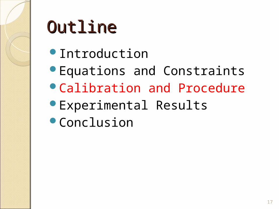
OutlineOutlineIntroductionEquations and ConstraintsCalibration and ProcedureExperimental ResultsConclusion
17

CalibrationCalibrationAnalytical solutionNonlinear optimization technique
based on the maximum-likelihood criterion
18

Closed-Form SolutionClosed-Form SolutionDefine B = A-TA-1 ≡
B is defined by 6D vector b
11 21 31
12 22 32
13 23 33
B B B
B B B
B B B
0 02 2 2
220 0 0
2 2 2 2 2 2 2
22 20 0 0 00 0 0 0
2 2 2 2 2 2 2
1
1
1
v u
v u v
v u v uv u v v
11 12 22 13 23 33
TB B B B B Bb
19
(5)
(6)

Closed-Form SolutionClosed-Form Solutionith column of H = hi
Following relation hold
1 2 3
T
i i i ih h hh
T Ti j ijh Bh v b
1 1 1 2 2 1 2 2 3 1 1 3 3 2 2 3 3 3
ij
T
i j i j i j i j i j i j i j i j i jh h h h h h h h h h h h h h h h h h
v
20
(7)

Closed-Form SolutionClosed-Form SolutionTwo fundamental constraints, from
homography, become
If observed n images of model plane
V is 2n x 6 matrixSolution of Vb = 0 is the eigenvector
of VTV associated w/ smallest eigenvalue
Therefore, we can estimate b
12
11 22
0T
T
vb
v v
0Vb
21
(8)
(9)

Closed-Form SolutionClosed-Form SolutionIf n ≥ 3, unique solution b defined
up to a scale factorIf n = 2, impose skewless
constraint γ = 0If n = 1, can only solve two camera
intrinsic parameters, α and β, assuming u0 and v0 are known and γ = 0
22
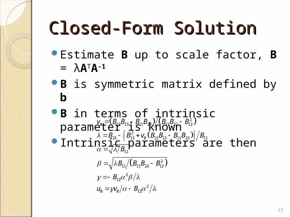
Closed-Form SolutionClosed-Form SolutionEstimate B up to scale factor, B =
λATA-1
B is symmetric matrix defined by bB in terms of intrinsic parameter is
knownIntrinsic parameters are then
20 12 13 11 23 11 22 12
233 13 0 12 13 11 23 11
11
211 11 22 12
212
20 0 13
v B B B B B B B
B B v B B B B B
B
B B B B
B
u v B
23

Closed-Form SolutionClosed-Form SolutionCalculating extrinsic parameter from
Homography H = [h1 h2 h3] = λA[r1 r2 t]
R = [r1 r2 r3] does not, in general, satisfy properties of a rotation matrix because of noise in data
R can be obtained through singular value decomposition
11 1 r A h 1
2 2 r A h 3 1 2 r r r 13 t A h
1 11 21 1 A h A h
24

Maximum-Likelihood Maximum-Likelihood EstimationEstimationGiven n images of model plane with m
points on model planeAssumption
◦ Corrupted Image points by independent and identically distributed noise
Minimizing following function yield maximum likelihood estimate
2
1 1
ˆ , , ,n m
ij i i ji j
m m
A R t M
25
(10)

Maximum-Likelihood Maximum-Likelihood EstimationEstimation is the projection of point
Mj in image iR is parameterized by a vector of three
parameters◦ Parallel to the rotation axis and magnitude is
equal to the rotation angleR and r are related by the Rodrigues
formulaNonlinear minimization problem solved
with Levenberg-Marquardt AlgorithmRequire initial guess
ˆ , , ,i i jm A R t M
26
, , t | 1..i i i nA R

Calibration ProcedureCalibration Procedure1. Print a pattern and attach to a planar
surface2. Take few images of the model plane
under different orientations3. Detect feature points in the images4. Estimate five intrinsic parameters
and all the extrinsic parameters using the closed-form solution
5. Refine all parameters by obtaining maximum-likelihood estimate
27

OutlineOutlineIntroductionEquations and ConstraintsCalibration and ProcedureExperimental ResultsConclusion
28
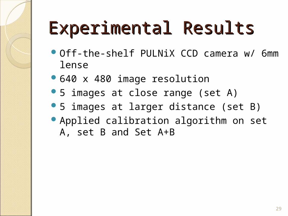
Experimental ResultsExperimental ResultsOff-the-shelf PULNiX CCD camera w/ 6mm
lense640 x 480 image resolution5 images at close range (set A)5 images at larger distance (set B)Applied calibration algorithm on set A, set B
and Set A+B
29

Experimental ResultExperimental Result
Angle b/w image axes
30

Experimental ResultExperimental Resulthttp://research.microsoft.com/en-us/um/people/zhahttp://research.microsoft.com/en-us/um/people/zhang/calib/ng/calib/
31
OutlineOutlineIntroductionEquations and ConstraintsCalibration and ProcedureExperimental ResultsConclusion
32
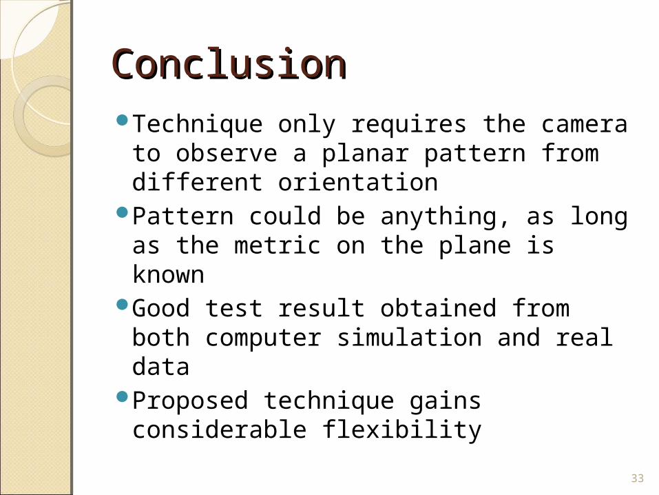
ConclusionConclusionTechnique only requires the camera
to observe a planar pattern from different orientation
Pattern could be anything, as long as the metric on the plane is known
Good test result obtained from both computer simulation and real data
Proposed technique gains considerable flexibility
33

AppendixAppendixEstimating Homography b/w the Model Plane and Estimating Homography b/w the Model Plane and its Imageits ImageMethod based on a maximum-
likelihood criterion (Other option available)
Let Mi and mi be the model and image point, respectively
Assume mi is corrupted by Gaussian noise with mean 0 and covariance matrix Λmi
34

AppendixAppendixMinimizing following function
yield maximum-likelihood estimation of H
where with = ith row of H
35
1ˆ ˆi
T
i i m i ii
m m m m
1
3 2
1ˆ
T
ii T T
i i
h Mm
h M h Mih

AppendixAppendixAssume for all iProblem become nonlinear least-
squares one, i.e. Nonlinear minimization is
conducted with Levenberg-Marquardt Algorithm that requires an initial guess with following procedure to obtain
36
2
imΛ I
2ˆmin i ii
H m m
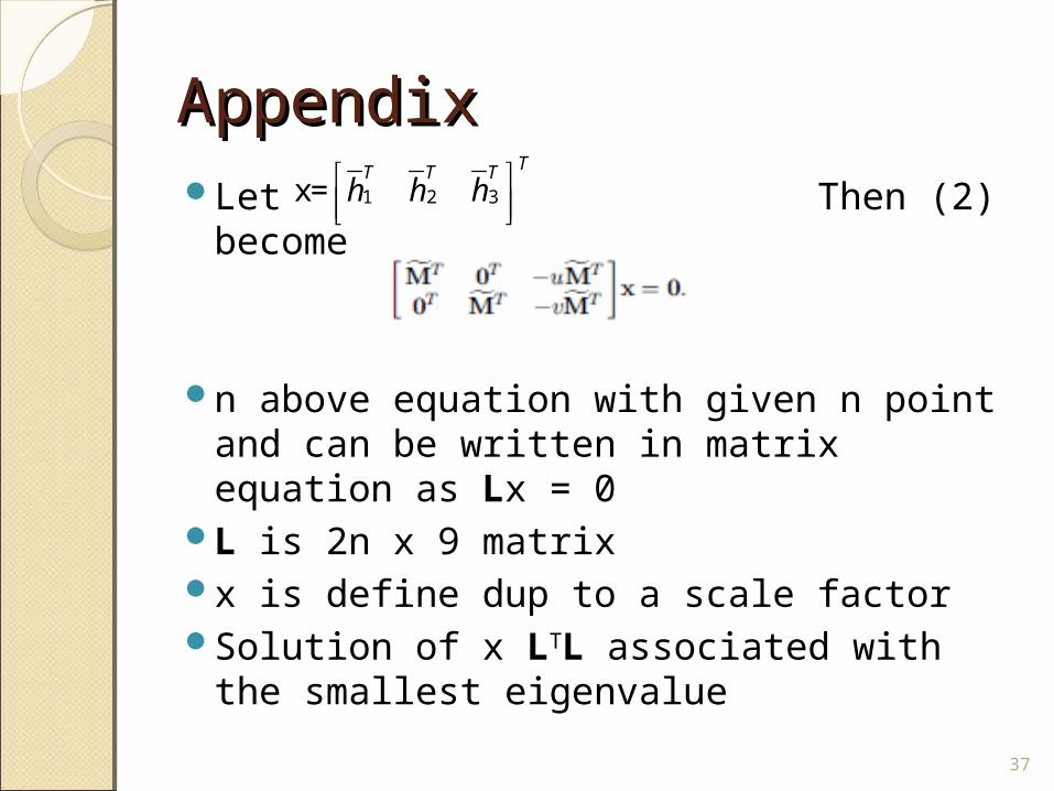
AppendixAppendixLet Then (2) become
n above equation with given n point and can be written in matrix equation as Lx = 0
L is 2n x 9 matrixx is define dup to a scale factorSolution of x LTL associated with the
smallest eigenvalue
37
1 2 3x=TT T T
h h h

AppendixAppendixElements of L
◦Constant 1◦Pixels◦World coordinates◦Multiplication of both
38

Possible Future WorkPossible Future WorkImproving distortion parameter
caused by lens distortion
39

Question?Question?
40