lable at ScienceDirect

Energy 98 (2016) 50e63

Contents lists avai

Energy

journal homepage: www.elsevier .com/locate/energy

A finite line source model with Cauchy-type top boundary conditionsfor simulating near surface effects on borehole heat exchangers

Jaime A. Rivera a, *, Philipp Blum b, Peter Bayer a

a ETH Zurich, Department of Earth Sciences, Sonneggstrasse 5, 8092 Zurich, Switzerlandb Karlsruhe Institute of Technology (KIT), Institute for Applied Geosciences (AGW), Kaiserstraße 12, 76131 Karlsruhe, Germany

a r t i c l e i n f o

Article history:Received 26 June 2015Received in revised form16 November 2015Accepted 12 December 2015Available online xxx

Keywords:Ground heat exchangeGround surface temperatureShallow geothermal energyFinite line sourceGround source heat pump

* Corresponding author. Tel.: þ41 44 6332594; fax:E-mail address: jaime.rivera@erdw.ethz.ch (J.A. Ri

http://dx.doi.org/10.1016/j.energy.2015.12.1290360-5442/© 2016 Elsevier Ltd. All rights reserved.

a b s t r a c t

BHEs (borehole heat exchangers) are the most common shallow geothermal applications. By approxi-mating the BHE as a line source, semi-analytical models can describe the heat exchange within theground. These models though always assume prescribed temperature at the ground surface. This workpresents a formulation which expands existing finite line source models by implementing a more generalCauchy-type top boundary condition and in this way, a better estimation of the heat fluxes at the groundsurface. The new formulation is numerically verified and examined in a dimensionless analysis. It isdemonstrated that the discrepancy to prescribed temperature settings is significant near to the groundsurface, and it propagates deeper when groundwater flow is absent and when strong decoupling be-tween the thermal regimes interacting at the land surface is assumed. The new approach shows to besuited especially for short BHEs, both for more flexible and accurate prediction of the ground thermalregime as well as for long-term analysis of technological performance.

© 2016 Elsevier Ltd. All rights reserved.

1. Introduction

The utilization of low-enthalpy geothermal energy focuses onthe shallow subsurface of some hundreds of metres depth. Mostcommonly, so-called ground heat exchangers or BHEs (boreholeheat exchangers) are installed. These exchange heat with theground by circulating a fluid through tubes installed in verticalboreholes. BHEs are usually connected to heat pumps defining theso-called GSHPs (ground source heat pump systems). During thelast decade, the number of BHEs has significantly grown, especiallyin cities of central and northern Europe, the USA and China [1,2]. In2015, worldwide annual utilization of GSHPs is estimated to reach325 PJ [3].

With their number and density growing, there is also risinginterest in improved simulation techniques to characterize andpredict the thermal response in the ground. The most elementarysimulation techniques are based on Kelvin's line source [4,5]. Forexample, the semi-analytical, infinite line-source solution is suit-able formodelling seasonal energy exchange. It treats the ground asan initially isothermal, homogeneous medium, where heat is

þ41 44 6331108.vera).

transported by conduction only. The BHE is approximated as avertical line of infinite length embedded in the ground. Dependingon the net thermal load on the system (net balance betweenheating and cooling loads), the line source creates a radial andexpanding temperature gradient during system operation. After atypical operational life span (between 30 and 50 years), the extentcan be up to tens of metres. On the long term, this may also affectneighbouring geothermal systems [6e10].

By approximating the ground as infinite conductive system, anyfurther processes and boundary conditions are neglected. These,however, have often shown to be crucial, and thus advanced linesource solutions have been proposed. Recent advancements inanalytical BHE modelling focus on improved expressions for moreefficient computer-based implementation, short term simulationand high time-resolution of operation with discontinuous heatextraction or injection [11e14]. Li and Lai [15,16] develop tech-niques to deal with anisotropy and heterogeneity of the sur-rounding mediumwith analytical models. One process is advectiveheat flux stimulated by horizontal groundwater flow. In fact, manyBHEs are installed in dynamic aquifers, so that even in aconduction-dominated environment, advection may have aremarkable influence on the evolution of ground temperaturesaround BHEs [17]. Thermal anomalies are deformed to heat or coldplumes elongated in downstream groundwater flow direction

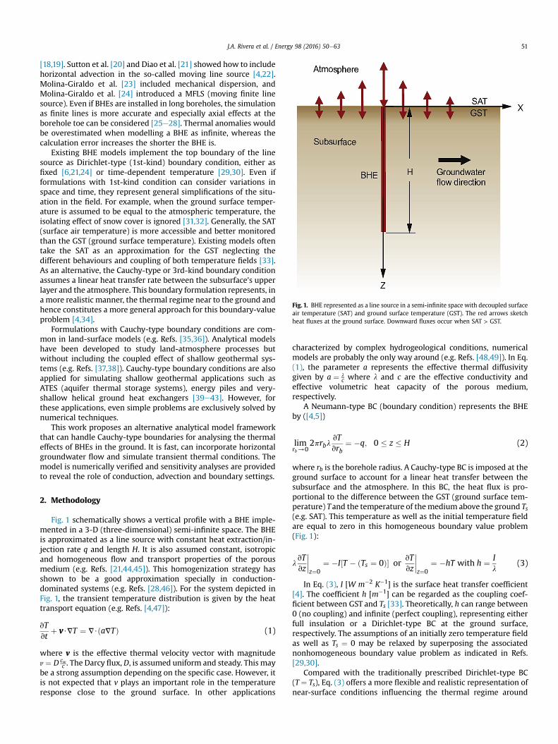
Fig. 1. BHE represented as a line source in a semi-infinite space with decoupled surfaceair temperature (SAT) and ground surface temperature (GST). The red arrows sketchheat fluxes at the ground surface. Downward fluxes occur when SAT > GST.

J.A. Rivera et al. / Energy 98 (2016) 50e63 51

[18,19]. Sutton et al. [20] and Diao et al. [21] showed how to includehorizontal advection in the so-called moving line source [4,22].Molina-Giraldo et al. [23] included mechanical dispersion, andMolina-Giraldo et al. [24] introduced a MFLS (moving finite linesource). Even if BHEs are installed in long boreholes, the simulationas finite lines is more accurate and especially axial effects at theborehole toe can be considered [25e28]. Thermal anomalies wouldbe overestimated when modelling a BHE as infinite, whereas thecalculation error increases the shorter the BHE is.

Existing BHE models implement the top boundary of the linesource as Dirichlet-type (1st-kind) boundary condition, either asfixed [6,21,24] or time-dependent temperature [29,30]. Even ifformulations with 1st-kind condition can consider variations inspace and time, they represent general simplifications of the situ-ation in the field. For example, when the ground surface temper-ature is assumed to be equal to the atmospheric temperature, theisolating effect of snow cover is ignored [31,32]. Generally, the SAT(surface air temperature) is more accessible and better monitoredthan the GST (ground surface temperature). Existing models oftentake the SAT as an approximation for the GST neglecting thedifferent behaviours and coupling of both temperature fields [33].As an alternative, the Cauchy-type or 3rd-kind boundary conditionassumes a linear heat transfer rate between the subsurface's upperlayer and the atmosphere. This boundary formulation represents, ina more realistic manner, the thermal regime near to the ground andhence constitutes a more general approach for this boundary-valueproblem [4,34].

Formulations with Cauchy-type boundary conditions are com-mon in land-surface models (e.g. Refs. [35,36]). Analytical modelshave been developed to study land-atmosphere processes butwithout including the coupled effect of shallow geothermal sys-tems (e.g. Refs. [37,38]). Cauchy-type boundary conditions are alsoapplied for simulating shallow geothermal applications such asATES (aquifer thermal storage systems), energy piles and very-shallow helical ground heat exchangers [39e43]. However, forthese applications, even simple problems are exclusively solved bynumerical techniques.

This work proposes an alternative analytical model frameworkthat can handle Cauchy-type boundaries for analysing the thermaleffects of BHEs in the ground. It is fast, can incorporate horizontalgroundwater flow and simulate transient thermal conditions. Themodel is numerically verified and sensitivity analyses are providedto reveal the role of conduction, advection and boundary settings.

2. Methodology

Fig. 1 schematically shows a vertical profile with a BHE imple-mented in a 3-D (three-dimensional) semi-infinite space. The BHEis approximated as a line source with constant heat extraction/in-jection rate q and length H. It is also assumed constant, isotropicand homogeneous flow and transport properties of the porousmedium (e.g. Refs. [21,44,45]). This homogenization strategy hasshown to be a good approximation specially in conduction-dominated systems (e.g. Refs. [28,46]). For the system depicted inFig. 1, the transient temperature distribution is given by the heattransport equation (e.g. Refs. [4,47]):

vTvt

þ v$VT ¼ V$ aVTð Þ (1)

where v is the effective thermal velocity vector with magnitudev ¼ D cw

c . The Darcy flux, D, is assumed uniform and steady. This maybe a strong assumption depending on the specific case. However, itis not expected that v plays an important role in the temperatureresponse close to the ground surface. In other applications

characterized by complex hydrogeological conditions, numericalmodels are probably the only way around (e.g. Refs. [48,49]). In Eq.(1), the parameter a represents the effective thermal diffusivitygiven by a ¼ l

c where l and c are the effective conductivity andeffective volumetric heat capacity of the porous medium,respectively.

A Neumann-type BC (boundary condition) represents the BHEby ([4,5])

limrb/0

2prblvTvrb

¼ �q; 0 � z � H (2)

where rb is the borehole radius. A Cauchy-type BC is imposed at theground surface to account for a linear heat transfer between thesubsurface and the atmosphere. In this BC, the heat flux is pro-portional to the difference between the GST (ground surface tem-perature) Tand the temperature of themedium above the ground Ts(e.g. SAT). This temperature as well as the initial temperature fieldare equal to zero in this homogeneous boundary value problem(Fig. 1):

lvTvz

����z¼0

¼ �I½T � ðTs ¼ 0Þ� orvTvz

����z¼0

¼ �hT with h ¼ Il

(3)

In Eq. (3), I [W m�2 K�1] is the surface heat transfer coefficient[4]. The coefficient h [m�1] can be regarded as the coupling coef-ficient between GST and Ts [33]. Theoretically, h can range between0 (no coupling) and infinite (perfect coupling), representing eitherfull insulation or a Dirichlet-type BC at the ground surface,respectively. The assumptions of an initially zero temperature fieldas well as Ts ¼ 0 may be relaxed by superposing the associatednonhomogeneous boundary value problem as indicated in Refs.[29,30].

Compared with the traditionally prescribed Dirichlet-type BC(T ¼ Ts), Eq. (3) offers a more flexible and realistic representation ofnear-surface conditions influencing the thermal regime around

J.A. Rivera et al. / Energy 98 (2016) 50e6352

BHEs. However, it needs to be emphasized that the new parameterh for specifying the Cauchy-type BC serves as surrogate of complexland-atmosphere processes, and so the obtained formulation is stillstrongly simplifying (e.g. Refs. [36,50]).

BCs as defined in Eq. (3) are common in numerical heat trans-port simulations to account for the effect of a rather thin layer thatrepresents the transition between the domain of interest (i.e. theground) and another medium with known temperature (i.e. theatmosphere) [51]. These known conditions can be transferred tothe boundary of a model by assigning a surface heat transfer co-efficient, I¼ lo/do, where lo is the thermal conductivity and do is thethickness of the transition layer. One shortcoming of this approachis that the thermal inertia of the transition layer is neglected. Still, itis a valuable model for approximating the effect of thin media suchas slabs and pavements within large scale models. These thin layersreach steady state thermal conditions relatively early, and thus theydo not need to be resolved as layers in the model.

Other near surface conditions such as an unsaturated zone couldbe accounted for in a similar way if its capacity to store and releaseheat is negligible. In this case, a sufficiently approximate approachmay be to resolve the temperature field in this zone assumingsaturated conditions (homogenization), since the thermal diffu-sivity does not change drastically with water content in porousmedia. Palmer et al. [40] for instance, based on the experimentalwork presented in Refs. [52], argued that thermal effects of anunsaturated zone are not appreciable for water contents between20% and 100%. More recently, Simms et al. [53] implemented nu-merical models to evaluate the effect of soil's thermal propertiesheterogeneity on the performance of horizontal ground heat ex-changers. For these very shallow systems, their results support thehomogenization approach since the impact of this heterogeneity isminimal compared with uncertainty of soils' mean thermal prop-erties. In general, close to the ground surface, the imposed BC islikely more dominant than potential effects induced by changes inwater content [54].

The problem posed in Eqs. (1)e(3) can be solved analytically bylinear superposition in space and time of unitary-instantaneousheat pulses according to the problem-specific Green's function.This is a common procedure for simulating BHEs with simple andcomplex Dirichlet-type BCs (e.g. Refs. [29,30,55,56]). In contrast,Cauchy-type BCs have been implemented only for simulating heattransfer at the borehole wall but not at the ground surface (e.g. Ref.[57]). The new analytical solution builds on a line source model andincorporates Eq. (3) as BC at the ground surface. For the systemshown in Fig. 1 it reads (see also Appendix A, Eq. (A11)):

Tðx; x0; tÞ ¼ TMFLSðx; x0; tÞ þ DThðx; x0; tÞ (4)

where TMFLS is the temperature calculated by the standard MFLS(moving finite line source) [24], and DTh is the contribution asso-ciated with Cauchy-type BC effects given by

DThðx; x0; tÞ ¼q

4lpexp�x� x0

2av

� Z∞r2d

4at

14exp�� 4�

�rdv4a

�214

�

�(exp

hzþ

�hrd2

�214

!�erfc

�zffiffiffi4

prd

þ hrd2ffiffiffi4

p�

� expðhHÞerfc�zþ Hrd

ffiffiffi4

p þ hrd2ffiffiffi4

p�)

d4

(5)

where r2d ¼ ðx� x0Þ2 þ ðy� y0Þ2.

Depending on the specific combination of parameters (x,x',t,h,a),the factor enclosed within the curly brackets in Eq. (5) can generatearithmetic overflow while evaluating the integral. One way aroundis to include the exponential factors within the complementary erfc(error function) through the following substitution (see alsoAppendix B, Eq. (B3)):

kðh;m; z; rdÞ ¼2rd

ffiffiffi4

p

r Z∞0

exp

"� hε� 4

�zþ mþ ε

rd

�2#dε (6)

which leads to reformulate Eq. (5) as

DThkðx; x0; tÞ ¼q

4lpexp�x� x

0

2av

� Z∞r2d

4at

14exp�� 4�

�rdv4a

�214

�

� ½kðh;0; z; rdÞ � kðh;H; z; rdÞ�d4(7)

The dimensionless forms of Eq. (4) can be written as

q X;X0;R; Pe; Fo

� �¼ qMFLS X;X

0;R; Pe; Fo

� �þ Dqh X;X

0;R; Pe; Fo;Hh

� �(8)

where q refers to dimensionless temperature. Alternatively, Dqh canbe expressed as Dqhk to avoid arithmetic overflow, and both for-mulations are included in the Appendix C (Eqs. (C1)e(C3)). In Eq.(8), the indicated dimensionless numbers including the P�ecletnumber Pe and the Fourier number Fo, are defined as follows

Pe ¼ vHa; Fo ¼ at

H2;�X;X

0� ¼�<X; Y ; Z > ; <X

0; Y

0; Z0 >

�

¼ 1H

�< x; y; z> ; < x

0; y

0; z

0>�; R ¼ rd

H; Hh ¼ hH

(9)

Eqs. (8)e(9) are employed in the next chapter to examine theeffect of the two boundary formulations on thermal plume evolu-tion around a BHE (i.e. on Dqh and qMFLS). Additionally, potentialimplications of simulation with Cauchy-type BC on optimal BHEsizing are addressed. For this, it is necessary to estimate the bore-hole wall temperature, which can be expressed through so-called‘g-functions’ as introduced by Eskilson [28,44] and thoroughlydiscussed in Refs. [58,59]. For single BHEs, an accepted metric forthis temperature is the mean borehole wall temperature (calcu-latedwith the finite line sourcemodel) as defined by Zeng et al. [45]and reformulated by Lamarche and Beauchamp [60]. Here, it isproposed an alternative formulation for the mean borehole walltemperature TMFLS which is based on the approach presented inRefs. [29,61]:

TMFLS ¼1

2prbH

Z2p0

ZH0

TMFLSrbdzdd ¼1

2pH

Z2p0

ZH0

TMFLSdzdd (10)

where dd is the differential angle in cylindrical coordinates andTMFLS is evaluated at the borehole radius. This alternative formu-lation reads:

J.A. Rivera et al. / Energy 98 (2016) 50e63 53

TMFLS ¼q

8lpI0

�RbPe2

� Z∞R2b

4Fo

14exp

"� 4�

�RbPe4

�214

#(4erf

� ffiffiffi4

pRb

�

� 2erf�2ffiffiffi4

pRb

�þ Rbffiffiffiffiffiffi

p4p

"4exp

� 4

R2b

!� exp

� 44

R2b

!

� 3

#)d4

(11)

where Rb ¼ rbH and I0 is the modified Bessel function of first kind and

of order zero. Since our interest is to quantify the net effect of Eq. (3)in the mean borehole temperature, Eq. (11) will be compared withan analogous expression derived from DTh (Eq. (5)):

DTh ¼ 12prbH

Z2p0

ZH0

DThrbdzdd ¼1

2pH

Z2p0

ZH0

DThdzdd (12)

DTh ¼ q4lp Hh

I0� rb2a

v� Z∞

r2b

4at

14exp�� 4�

�rbv4a

�214

�jðh;H; rb;4Þd4

(13)

jðh;H; rb;4Þ ¼ 2erf�Hrb

ffiffiffi4

p �� erf

�2Hrb

ffiffiffi4

p �þ exp

"�hrb2

�214

#

��expðhHÞerfc

�Hrb

ffiffiffi4

p þ hrb2ffiffiffi4

p�� erfc

�hrb2ffiffiffi4

p�

� expð2hHÞerfc�2Hrb

ffiffiffi4

p þ hrb2ffiffiffi4

p�

þ expðhHÞerfc�Hrb

ffiffiffi4

p þ hrb2ffiffiffi4

p�

(14)

Alternatively, the function jðh;H; rb;4Þ in Eq. (14) can beexpressed in terms of kðh;m; z; rdÞ (Eq. (6)) as follows:

jkðh;H; rb;4Þ ¼ 2erf�Hrb

ffiffiffi4

p �� erf

�2Hrb

ffiffiffi4

p �þ kðh;H;0; rbÞ

� kðh;0;0; rbÞ � kðh;H;H; rbÞ þ kðh;0;H; rbÞ(15)

In Eqs. 13e15, the dimensionless groups shown in Eq. (9) canalso be identified. The corresponding dimensionless forms Dqh, Jand JΚ are listed in Appendix C (Eqs. (C4)e(C6)).

In order to compare Dqh with the dimensionless form of Eq. (11)(qMFLS), we have qMFLS ¼ 4lpTMFLS=q.

Finally, a comparison between Dirichlet- and Cauchy-type BCs iscarried out by inspecting their effect on the overall ground energybalance during BHE operation. Following the analysis in Rivera at al.[62], the time-dependent power supplied and loss through the topboundary, pðz ¼ 0; tÞ; is obtained by integrating the vertical heatfluxes over the entire top surface:

pðz ¼ 0; tÞ ¼Z∞�∞

Z∞�∞

l

�vTvz

�z¼0

dxdy ¼Z∞�∞

Z∞�∞

IðDThÞz¼0dxdy

(16)

where Eqs. (3) and (4) are merged taking into account that TMFLS isalways zero at the top surface, and the assumption Ts ¼ 0 (homo-geneous boundary-value problem). The triple integral in Eq. (16)can be simplified as follows [62]:

pðz ¼ 0; tÞ ¼ hqH2

4

Z∞H24at

142 exp

"�hH2

�214

#�erfc

�hH2ffiffiffi4

p�

� expðhHÞerfc� ffiffiffi

4p þ hH

2ffiffiffi4

p�

d4 (17)

or alternatively in terms of the function k (Eq. (6)):

pðz ¼ 0; tÞ ¼ hqH2

4

Z∞H24at

142 ½kðh;0;0;HÞ � kðh;H;0;HÞ�d4 (18)

The dimensionless form of the total power is thenP(Fo, Hh) ¼ p(z ¼ 0,t)/qH where Fo (appearing in the lower limit ofthe integral) and Hh are defined in Eq. (9).

In the next chapter, the proposed analytical framework isnumerically verified and its role elucidated via a sensitivity analysisbased on the identified dimensionless groups. For this, focus is seton thermal plumes, mean borehole temperatures (g-functions) andpower supplied to the BHE through the top boundary.

3. Results and discussion

3.1. Numerical verification

A fundamental first step for proving the correctness of theproposed model is its numerical verification. For this, the syntheticsetup shown in Fig. 1 is simulated using a finite element heattransport model (FEFLOW version 6.2 [51]). Temperature depthprofiles (TDPs) are taken at different locations and times, and theseare compared to analytical results obtained by Eqs. (4)e(7).

The physical and thermal properties of the porous medium arechosen so that they represent typical values for sandy aquifers [17]:effective porosity ne ¼ 0.25, bulk thermal conductivityl ¼ 2.4 W m�1 K�1, and volumetric heat capacity of the porousmedium c ¼ 2.7 MJ K�1 m�3. For this verification, the heat rate atthe borehole is set to q ¼ �30 W m�1 (heating) with a lengthH ¼ 50 m. The BHE is simulated in FEFLOW via a linear (vertical)DFE (discrete feature element) that connects multiple nodal sour-ces with equal heat rate (4th kind BC).

FEFLOW allows the implementation of Cauchy-type BC at theground surface by assigning an input/output heat transfer coeffi-cient to the upper most numerical layer. In this exercise, this co-efficient is I ¼ 1 W m�2 K�1 which implies a heat exchange rateh ¼ I/l ¼ 0.4 m�1. Additionally, in the numerical model it isnecessary to assign the known temperature of the medium abovethe ground to the grid nodes constituting the uppermost numericalslice (i.e. the ground surface). This temperature, as well as the initialtemperature in the domain, are set equal to zero according to themodel assumptions (Fig. 2). The size of the numerical model ischosen so that lateral and bottom boundary effects are negligible. Inthe vertical direction, the 100 m depth synthetic aquifer is dis-cretised in 142 layers with varying thickness. For the first 55 m, thelayers are 0.5 m thick in order to resolve properly the top boundaryeffects. Then the thickness of the layers is increased to 1 m fordepths between 55 m and 70 m, and to 2 m thickness onwards. Inthe horizontal plane, an area of 200 m � 100 m is discretised in

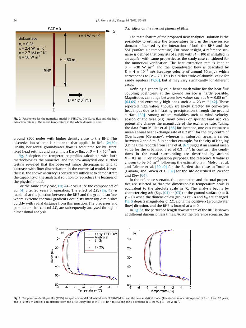
Fig. 2. Parameters for the numerical model in FEFLOW. D is Darcy flux and the heatextraction rate is q. The initial temperature in the whole domain is zero.

J.A. Rivera et al. / Energy 98 (2016) 50e6354

around 8500 nodes with higher density close to the BHE. Thisdiscretization scheme is similar to that applied in Refs. [24,30].Finally, horizontal groundwater flow is accounted for by lateralfixed head settings and assuming a Darcy flux of D ¼ 1 � 10�7 m/s.

Fig. 3 depicts the temperature profiles calculated with bothmethodologies, the numerical and the new analytical one. Furthertesting revealed that the observed minor discrepancies tend todecrease with finer discretization in the numerical model. Never-theless, the shown accuracy is considered sufficient to demonstratethe capability of the analytical solution to reproduce the features ofthe physical model.

For the same study case, Fig. 4aec visualize the components ofEq. (4) after 20 years of operation. The effect of DTh (Fig. 4a) ismaximal at the junction between the BHE and the ground surface,where extreme thermal gradients occur. Its intensity diminishesquickly with radial distance from this junction. The processes andparameters that control DTh are subsequently analysed through adimensional analysis.

Fig. 3. Temperature-depth profiles (TDPs) for synthetic model calculated with FEFLOW (dotsand (a) at 0.5 m and (b) 1 m distance from the BHE; Darcy flux is D ¼ 1 � 10�7 m/s (along

3.2. Effect on the thermal plumes of BHEs

The main feature of the proposed new analytical solution is thepossibility to estimate the temperature field in the near-surfacedomain influenced by the interaction of both the BHE and theSAT (surface air temperature). For more insight, a reference sce-nario is defined that consists of a BHE with H ¼ 100 m installed inan aquifer with same properties as the study case considered forthe numerical verification. The heat extraction rate is kept atq ¼ �30 W m�1 and the groundwater flow is described byD ¼ 4 � 10�7 m/s (seepage velocity of around 50 m/y), whichcorresponds to Pe ¼ 70. This is a rather “rule-of-thumb” value forsandy aquifers [17,63], but it may vary significantly for differentcases.

Defining a generally valid benchmark value for the heat fluxcoupling coefficient at the ground surface is hardy possible.Magnitudes can range between low values such as h z 0.05 m�1

[64,65] and extremely high ones such h ¼ 23 m�1 [42]. Thosereported high values though are likely affected by convectiveheat input due to infiltrating precipitation through the groundsurface [39]. Among others, variables such as wind velocity,season of the year (e.g. snow cover) or specific land use canpotentially change the magnitude of the exchange rate. Takingthe data from Müller et al. [66] for instance, one can estimate amean annual heat exchange rate of 0.2 m�1 for the city centre ofOberhausen (Germany), whereas in suburban areas, h rangesbetween 2 and 8 m�1. In another example, for the city of Nanjing(China), the records from Tang et al. [67] suggest an annual meanvalue for the urbanized area of 0.3 m�1. In contrast, the condi-tions in the rural surrounding are described by aroundh ¼ 0.1 m�1. For comparison purposes, the reference h value ischosen to be 0.5 m�1 following the estimations in Molson et al.and Palmer et al. [39,40] for the Borden site close to Toronto(Canada) and Güven et al. [37] for the site described in Wernerand Kley [64].

In the reference scenario, the parameters and thermal proper-ties are selected so that the dimensionless temperature scale isequivalent to the absolute scale in �C. The analysis begins bycharacterizing Dqh (Eqs. (C1) or (C3)) at the ground surface (z ¼ 0,y ¼ 0) when the dimensionless groups Pe, Fo and Hh are changed.Fig. 5 depicts magnitudes of Dqh along the positive x (groundwaterflow) direction, and the BHE is located at x ¼ 0.

In Fig. 5a, the perturbed length downstream of the BHE is shownat different dimensionless times, Fo. For the reference scenario, the

) and the new analytical model (lines) after an operation period of t ¼ 1, 2 and 20 years,the x direction), H ¼ 50 m, q ¼ �30 W m�1.

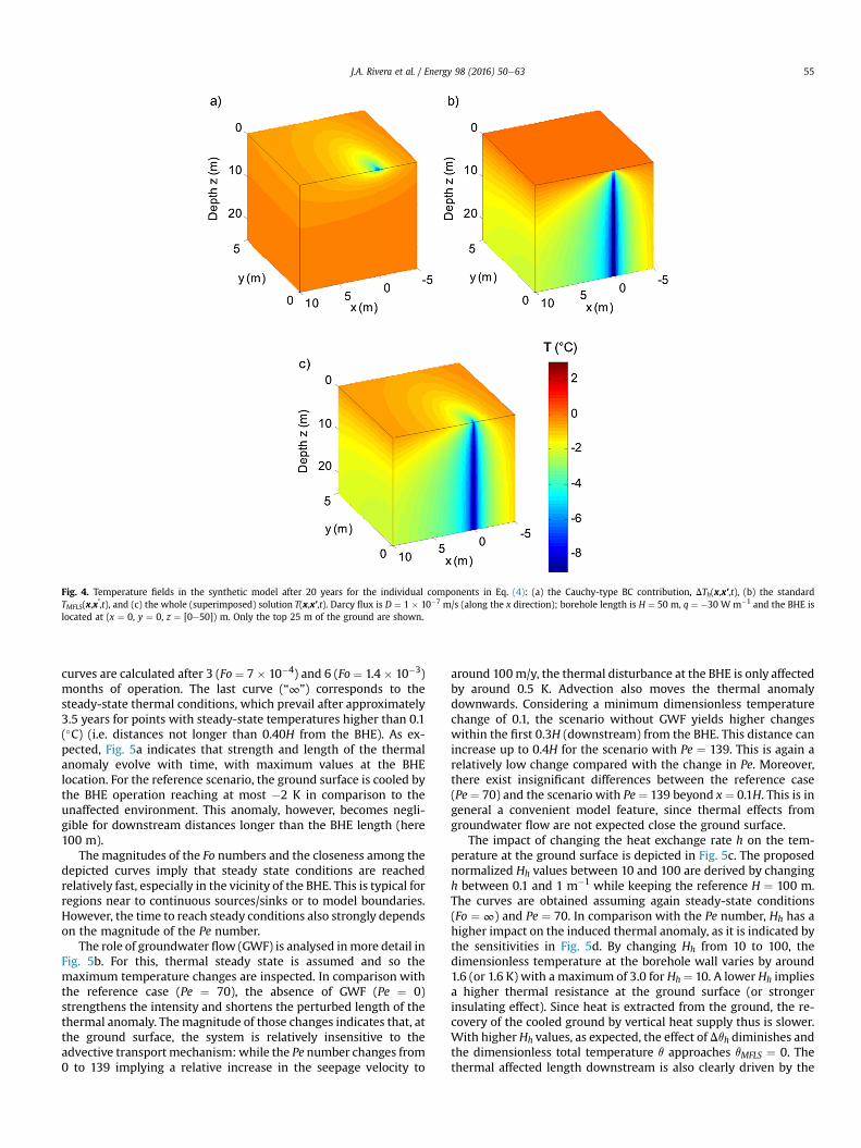
Fig. 4. Temperature fields in the synthetic model after 20 years for the individual components in Eq. (4): (a) the Cauchy-type BC contribution, DTh(x,x',t), (b) the standardTMFLS(x,x',t), and (c) the whole (superimposed) solution T(x,x',t). Darcy flux is D ¼ 1 � 10�7 m/s (along the x direction); borehole length is H ¼ 50 m, q ¼ �30 W m�1 and the BHE islocated at (x ¼ 0, y ¼ 0, z ¼ [0e50]) m. Only the top 25 m of the ground are shown.

J.A. Rivera et al. / Energy 98 (2016) 50e63 55

curves are calculated after 3 (Fo¼ 7 � 10�4) and 6 (Fo ¼ 1.4 � 10�3)months of operation. The last curve (“∞”) corresponds to thesteady-state thermal conditions, which prevail after approximately3.5 years for points with steady-state temperatures higher than 0.1(�C) (i.e. distances not longer than 0.40H from the BHE). As ex-pected, Fig. 5a indicates that strength and length of the thermalanomaly evolve with time, with maximum values at the BHElocation. For the reference scenario, the ground surface is cooled bythe BHE operation reaching at most �2 K in comparison to theunaffected environment. This anomaly, however, becomes negli-gible for downstream distances longer than the BHE length (here100 m).

The magnitudes of the Fo numbers and the closeness among thedepicted curves imply that steady state conditions are reachedrelatively fast, especially in the vicinity of the BHE. This is typical forregions near to continuous sources/sinks or to model boundaries.However, the time to reach steady conditions also strongly dependson the magnitude of the Pe number.

The role of groundwater flow (GWF) is analysed inmore detail inFig. 5b. For this, thermal steady state is assumed and so themaximum temperature changes are inspected. In comparison withthe reference case (Pe ¼ 70), the absence of GWF (Pe ¼ 0)strengthens the intensity and shortens the perturbed length of thethermal anomaly. Themagnitude of those changes indicates that, atthe ground surface, the system is relatively insensitive to theadvective transport mechanism: while the Pe number changes from0 to 139 implying a relative increase in the seepage velocity to

around 100m/y, the thermal disturbance at the BHE is only affectedby around 0.5 K. Advection also moves the thermal anomalydownwards. Considering a minimum dimensionless temperaturechange of 0.1, the scenario without GWF yields higher changeswithin the first 0.3H (downstream) from the BHE. This distance canincrease up to 0.4H for the scenario with Pe ¼ 139. This is again arelatively low change compared with the change in Pe. Moreover,there exist insignificant differences between the reference case(Pe¼ 70) and the scenario with Pe¼ 139 beyond x ¼ 0.1H. This is ingeneral a convenient model feature, since thermal effects fromgroundwater flow are not expected close the ground surface.

The impact of changing the heat exchange rate h on the tem-perature at the ground surface is depicted in Fig. 5c. The proposednormalized Hh values between 10 and 100 are derived by changingh between 0.1 and 1 m�1 while keeping the reference H ¼ 100 m.The curves are obtained assuming again steady-state conditions(Fo ¼ ∞) and Pe ¼ 70. In comparison with the Pe number, Hh has ahigher impact on the induced thermal anomaly, as it is indicated bythe sensitivities in Fig. 5d. By changing Hh from 10 to 100, thedimensionless temperature at the borehole wall varies by around1.6 (or 1.6 K) with a maximum of 3.0 for Hh ¼ 10. A lower Hh impliesa higher thermal resistance at the ground surface (or strongerinsulating effect). Since heat is extracted from the ground, the re-covery of the cooled ground by vertical heat supply thus is slower.With higher Hh values, as expected, the effect of Dqh diminishes andthe dimensionless total temperature q approaches qMFLS ¼ 0. Thethermal affected length downstream is also clearly driven by the

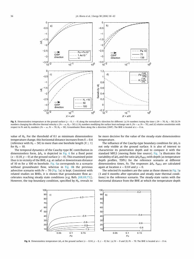
Fig. 5. Dimensionless temperature at the ground surface (y ¼ 0, z ¼ 0) along the normalized x direction for different: (a) Fo numbers tuning the time t, (Pe ¼ 70, Hh ¼ 50) (b) Penumbers changing the effective thermal velocity v, (Fo ¼∞, Hh ¼ 50) (c) Hh numbers modifying the surface heat exchange rate h, (Fo ¼∞, Pe ¼ 70), and (d) relative sensitivities withrespect to Pe and Hh numbers (Fo ¼ ∞, Pe ¼ 70, Hh ¼ 50). Groundwater flows along the x direction (GWF). The BHE is located at x ¼ 0 m.

J.A. Rivera et al. / Energy 98 (2016) 50e6356

value of Hh. For the threshold of 0.1 as minimum dimensionlesstemperature change, this horizontal distance increases from X¼ 0.4(reference with Hh ¼ 50) to more than one borehole length (X � 1)for Hh ¼ 10.

The temporal dynamics of the Cauchy-type BC contribution indimensionless form, Dqh, is depicted in Fig. 6 for a fixed point(x¼ 0.1H, y¼ 0) at the ground surface (z¼ 0). This examined pointthus is in vicinity of the BHE, e.g. at radial or downstream distanceof 10 m for a 100 m borehole. Fig. 6a corresponds to a scenariowithout groundwater flow, whereas in Fig. 6b the previousadvective scenario with Pe ¼ 70 (Fig. 5a) is kept. Consistent withrelated studies on BHEs, it is shown that groundwater flow ac-celerates reaching steady state conditions (e.g. Refs. [68,69,73]).However, the top boundary condition, specified by Hh, reveals to

Fig. 6. Dimensionless temperature Dqh at the ground surface (x ¼ 0.1H, y ¼

be more decisive for the value of the steady-state dimensionlesstemperature.

The influence of the Cauchy-type boundary condition for Dqh isnot only visible at the ground surface. It is also of interest tocharacterize its penetration depth and to compare it with thestandard MFLS (moving finite line source). Fig. 7a illustrates thevariability ofDqh and the ratioDqh/qMFLSwith depth (as temperaturedepth profiles, TDPs) for the reference scenario at differentdimensionless times, Fo. The responses Dqh, qMFLS are calculatedagain at location x ¼ 0.1H and y ¼ 0.

The selected Fo numbers are the same as those shown in Fig. 5a(3 and 6 months after operation and steady state thermal condi-tions) in the reference scenario. The steady-state varies with thehorizontal distance from the BHE at which the temperature depth

0, z ¼ 0) for: (a) Pe ¼ 0 and (b) Pe ¼ 70. The BHE is located at x ¼ 0 m.

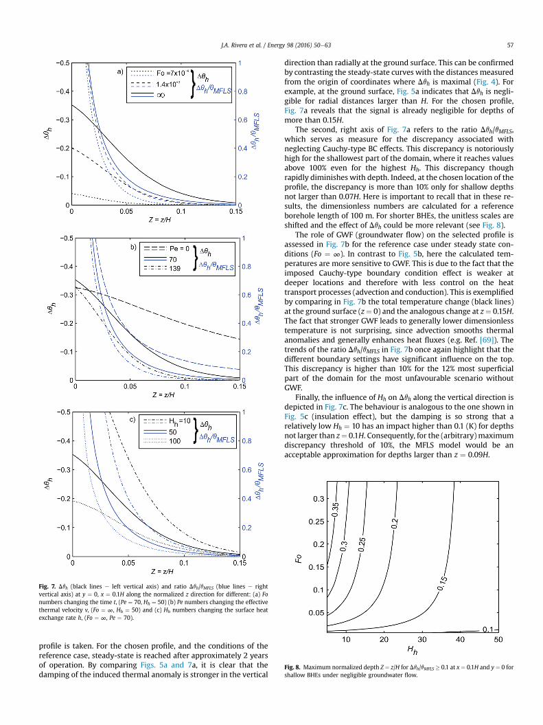
Fig. 7. Dqh (black lines e left vertical axis) and ratio Dqh/qMFLS (blue lines e rightvertical axis) at y ¼ 0, x ¼ 0.1H along the normalized z direction for different: (a) Fonumbers changing the time t, (Pe ¼ 70, Hh ¼ 50) (b) Pe numbers changing the effectivethermal velocity v, (Fo ¼ ∞, Hh ¼ 50) and (c) Hh numbers changing the surface heatexchange rate h, (Fo ¼ ∞, Pe ¼ 70).

Fig. 8. Maximum normalized depth Z ¼ z/H for Dqh/qMFLS � 0.1 at x ¼ 0.1H and y ¼ 0 forshallow BHEs under negligible groundwater flow.

J.A. Rivera et al. / Energy 98 (2016) 50e63 57

profile is taken. For the chosen profile, and the conditions of thereference case, steady-state is reached after approximately 2 yearsof operation. By comparing Figs. 5a and 7a, it is clear that thedamping of the induced thermal anomaly is stronger in the vertical

direction than radially at the ground surface. This can be confirmedby contrasting the steady-state curves with the distances measuredfrom the origin of coordinates where Dqh is maximal (Fig. 4). Forexample, at the ground surface, Fig. 5a indicates that Dqh is negli-gible for radial distances larger than H. For the chosen profile,Fig. 7a reveals that the signal is already negligible for depths ofmore than 0.15H.

The second, right axis of Fig. 7a refers to the ratio Dqh/qMFLS,which serves as measure for the discrepancy associated withneglecting Cauchy-type BC effects. This discrepancy is notoriouslyhigh for the shallowest part of the domain, where it reaches valuesabove 100% even for the highest Hh. This discrepancy thoughrapidly diminishes with depth. Indeed, at the chosen location of theprofile, the discrepancy is more than 10% only for shallow depthsnot larger than 0.07H. Here is important to recall that in these re-sults, the dimensionless numbers are calculated for a referenceborehole length of 100 m. For shorter BHEs, the unitless scales areshifted and the effect of Dqh could be more relevant (see Fig. 8).

The role of GWF (groundwater flow) on the selected profile isassessed in Fig. 7b for the reference case under steady state con-ditions (Fo ¼ ∞). In contrast to Fig. 5b, here the calculated tem-peratures are more sensitive to GWF. This is due to the fact that theimposed Cauchy-type boundary condition effect is weaker atdeeper locations and therefore with less control on the heattransport processes (advection and conduction). This is exemplifiedby comparing in Fig. 7b the total temperature change (black lines)at the ground surface (z¼ 0) and the analogous change at z¼ 0.15H.The fact that stronger GWF leads to generally lower dimensionlesstemperature is not surprising, since advection smooths thermalanomalies and generally enhances heat fluxes (e.g. Ref. [69]). Thetrends of the ratio Dqh/qMFLS in Fig. 7b once again highlight that thedifferent boundary settings have significant influence on the top.This discrepancy is higher than 10% for the 12% most superficialpart of the domain for the most unfavourable scenario withoutGWF.

Finally, the influence of Hh on Dqh along the vertical direction isdepicted in Fig. 7c. The behaviour is analogous to the one shown inFig. 5c (insulation effect), but the damping is so strong that arelatively low Hh ¼ 10 has an impact higher than 0.1 (K) for depthsnot larger than z¼ 0.1H. Consequently, for the (arbitrary)maximumdiscrepancy threshold of 10%, the MFLS model would be anacceptable approximation for depths larger than z ¼ 0.09H.

J.A. Rivera et al. / Energy 98 (2016) 50e6358

The results shown in Fig. 7 were obtained assuming a refer-ence length of H ¼ 100 m. Since Dqh is not linear with respect toHh, it is worth quantifying the effect on more shallow BHEs. Fig. 8shows the maximum normalized depth at which Dqh/qMFLS �0.1(or 10% discrepancy threshold) assuming no groundwater flow(unfavourable case) and a thermal profile taken at x ¼ 0.1H andy ¼ 0. The discrepancy threshold is given as function of Fo andHh.

For the considered range of Hh, Fig. 8 indicates that qMFLS is anacceptable surrogate to q (less than 10% discrepancy) fornormalized depths of z > 0.1H (minor insulation) and z > 0.35H(strong insulation). Taken for instance an energy pile withH ¼ 20 m such as the one analysed by Loveridge and Powrie [70]and the moderate reference case with h ¼ 0.5 m�1, Fig. 8 impliesthat the MFLS is not acceptable for estimating the temperatureat depths ranging between z ¼ 0 and z ¼ 0.3H ¼ 6 m at themedium term (Fo � 0.1). Of course, the line source model is notthe best approach for describing energy piles, where geometryand the thermal inertia of the fill material are important issues.However, since shallower geothermal systems (e.g. energy pilesand coils) are even more affected by the thermal conditions atthe ground surface than BHEs, the proposed Cauchy-type BCmight be suited to improve existing analytical models (e.g. Refs.[16,56,68,71,72]).

3.3. Effect on the mean borehole wall temperature and total powersupply from the ground surface

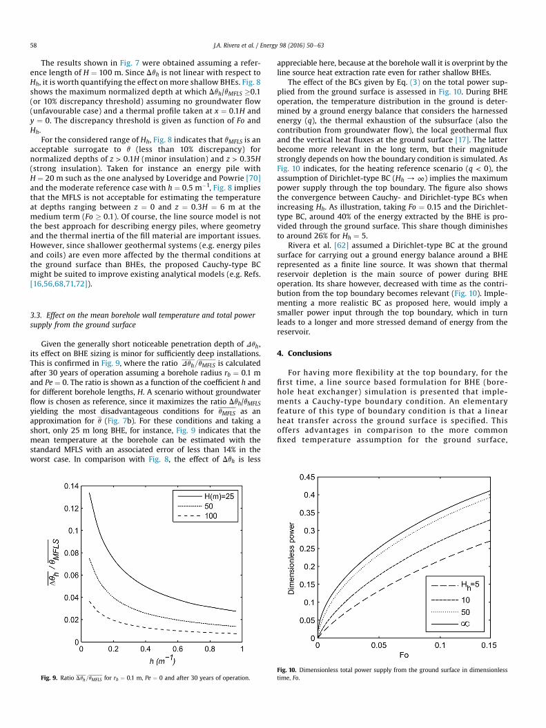
Given the generally short noticeable penetration depth of Dqh,its effect on BHE sizing is minor for sufficiently deep installations.This is confirmed in Fig. 9, where the ratio Dqh=qMFLS is calculatedafter 30 years of operation assuming a borehole radius rb ¼ 0.1 mand Pe ¼ 0. The ratio is shown as a function of the coefficient h andfor different borehole lengths, H. A scenario without groundwaterflow is chosen as reference, since it maximizes the ratio Dqh/qMFLS

yielding the most disadvantageous conditions for qMFLS as anapproximation for q (Fig. 7b). For these conditions and taking ashort, only 25 m long BHE, for instance, Fig. 9 indicates that themean temperature at the borehole can be estimated with thestandard MFLS with an associated error of less than 14% in theworst case. In comparison with Fig. 8, the effect of Dqh is less

Fig. 9. Ratio Dqh=qMFLS for rb ¼ 0.1 m, Pe ¼ 0 and after 30 years of operation.

appreciable here, because at the borehole wall it is overprint by theline source heat extraction rate even for rather shallow BHEs.

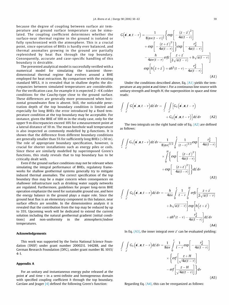
The effect of the BCs given by Eq. (3) on the total power sup-plied from the ground surface is assessed in Fig. 10. During BHEoperation, the temperature distribution in the ground is deter-mined by a ground energy balance that considers the harnessedenergy (q), the thermal exhaustion of the subsurface (also thecontribution from groundwater flow), the local geothermal fluxand the vertical heat fluxes at the ground surface [17]. The latterbecome more relevant in the long term, but their magnitudestrongly depends on how the boundary condition is simulated. AsFig. 10 indicates, for the heating reference scenario (q < 0), theassumption of Dirichlet-type BC (Hh / ∞) implies the maximumpower supply through the top boundary. The figure also showsthe convergence between Cauchy- and Dirichlet-type BCs whenincreasing Hh. As illustration, taking Fo ¼ 0.15 and the Dirichlet-type BC, around 40% of the energy extracted by the BHE is pro-vided through the ground surface. This share though diminishesto around 26% for Hh ¼ 5.

Rivera et al. [62] assumed a Dirichlet-type BC at the groundsurface for carrying out a ground energy balance around a BHErepresented as a finite line source. It was shown that thermalreservoir depletion is the main source of power during BHEoperation. Its share however, decreased with time as the contri-bution from the top boundary becomes relevant (Fig. 10). Imple-menting a more realistic BC as proposed here, would imply asmaller power input through the top boundary, which in turnleads to a longer and more stressed demand of energy from thereservoir.

4. Conclusions

For having more flexibility at the top boundary, for thefirst time, a line source based formulation for BHE (bore-hole heat exchanger) simulation is presented that imple-ments a Cauchy-type boundary condition. An elementaryfeature of this type of boundary condition is that a linearheat transfer across the ground surface is specified. Thisoffers advantages in comparison to the more commonfixed temperature assumption for the ground surface,

Fig. 10. Dimensionless total power supply from the ground surface in dimensionlesstime, Fo.

J.A. Rivera et al. / Energy 98 (2016) 50e63 59

because the degree of coupling between surface air tem-perature and ground surface temperature can be simu-lated. The coupling coefficient determines whether thesurface-near thermal regime in the ground is isolated orfully synchronized with the atmosphere. This is a crucialpoint, since operation of BHEs is hardly ever balanced, andthermal anomalies growing in the ground are partiallyreplenished by heat flux through the top boundary.Consequently, accurate and case-specific handling of thisboundary is desirable.

The presented analytical model is successfully verified with anumerical model for simulating the transient three-dimensional thermal regime that evolves around a BHEemployed for heat extraction. By comparison with the existingstandard MFLS, it is revealed that in shallow depths the dis-crepancies between simulated temperatures are considerable.For the verification case, for example it is expected 2e4 K colderconditions for the Cauchy-type close to the ground surface.These differences are generally more pronounced when hori-zontal groundwater flow is absent. Still, the noticeable pene-tration depth of the top boundary condition is limited andespecially for long BHEs the error introduced by a fixed tem-perature condition at the top boundary may be acceptable. Forinstance, given the BHE of 100 m in the study case, only for theupper 9 m discrepancies exceed 10% for a measurement point ata lateral distance of 10 m. The mean borehole wall temperatureis also inspected as commonly modelled by g-functions. It isshown that the difference from different boundary conditionsare generally smaller than 5% for sufficiently long BHEs (>50 m).The role of appropriate boundary specification, however, iscrucial for shorter installations such as energy piles or coils.Since these are similarly modelled by superimposed Green'sfunctions, this study reveals that to top boundary has to becritically dealt with.

Even if the ground surface conditions may not be relevant whensimulating the integral performance of BHEs, regulatory frame-works for shallow geothermal systems generally try to mitigateinduced thermal anomalies. The correct specification of the topboundary thus may be a major concern when consequences onshallower infrastructure such as drinking water supply networksare regulated. Furthermore, guidelines for proper long-term BHEoperation emphasize the need for sustainable ground use, and herethe energy balance in the ground plays a major role. Since theground heat flux is an elementary component in this balance, nearsurface effects are sensible. In the dimensionless analysis it isrevealed that the contribution from the top may be reduced by upto 35%. Upcoming work will be dedicated to extend the currentsolution including the natural geothermal gradient (initial condi-tions) and non-uniformity in the atmospheric/indoortemperatures.

Acknowledgements

This work was supported by the Swiss National Science Foun-dation (SNSF) under grant number 200021L 144288, and theGerman Research Foundation (DFG), under grant number BL 1015/4-1.

Appendix A

For an unitary and instantaneous energy pulse released at thepoint x0 and time t in a semi-infinite and homogeneous domainwith specified coupling coefficient h through the top boundary,Carslaw and Jeager [4] defined the following Green's function:

G�x

0; x; t � t

�¼ 1

8½apðt � tÞ�32

(exp

"�z� z

0�24aðt � tÞ

#

þ exp

"�zþ z

0�24aðt � tÞ

#)exp

"� r2d4aðt � tÞ

#

� h4apðt � tÞ erfc

"zþ z

0

2ffiffiffiffiffiffiffiffiffiffiffiffiffiffiffiffiffiaðt � tÞp þ h

ffiffiffiffiffiffiffiffiffiffiffiffiffiffiffiffiffiaðt � tÞ

p #

exp

"h�zþ z

0�þ ah2ðt � tÞ � r2d4aðt � tÞ

#

(A1)

Under the conditions described above, Eq. (A1) yields the tem-perature at any point x and time t. For a continuous line sourcewithunitary strength and length H, the superposition in space and timereads:

Zt

Zz0

G�x

0; x; t � t

�dz

0dt ¼

Zt

Zz0

hG1

�x

0; x; t � t

�

þ G2

�x

0; x; t � t

�idz

0dt (A2)

The two integrals on the right hand side of Eq. (A2) are definedas follows:

Zt

Zz0

G1

�x

0;x;t�t

�dz

0dt¼ 1

8½ap�3=2Zt0

1

ðt�tÞ3=2exp

"� r2d4aðt�tÞ

#

�ZH0

(exp

"�z�z

0�24aðt�tÞ

#

þexp

"�zþz

0�24aðt�tÞ

#)dz

0dt

(A3)

Zt

Zz0

G2

�x

0; x; t � t

�dz

0dt ¼ � h

4ap

Zt0

1t � t

ZH0

erfc

"zþ z

0

2ffiffiffiffiffiffiffiffiffiffiffiffiffiffiffiffiffiaðt � tÞp

þ hffiffiffiffiffiffiffiffiffiffiffiffiffiffiffiffiffiaðt � tÞ

p #exp

"h�zþ z

0�

þ ah2ðt � tÞ � r2d4aðt � tÞ

#dz

0dt

(A4)

In Eq. (A3), the inner integral over z0 can be evaluated yielding:

Zt

Zz0

G1

�x

0; x; t � t

�dz

0dt ¼ 1

8ap

Zt0

1t � t

exp

"� r2d4aðt � tÞ

#

�(erf

"zþ Hffiffiffiffiffiffiffiffiffiffiffiffiffiffiffiffiffiffiffiffi4aðt � tÞp

#

� erf

"z� Hffiffiffiffiffiffiffiffiffiffiffiffiffiffiffiffiffiffiffiffi4aðt � tÞp

#)dt

(A5)

Regarding Eq. (A4), this can be reorganized as follows:

J.A. Rivera et al. / Energy 98 (2016) 50e6360

Zt

Zz0

G2

�x

0; x; t � t

�dz

0dt ¼ � h

4ap

Zt0

1t � t

exp

"ah2ðt � tÞ

� r2d4aðt � tÞ

#ZH0

erfc

"zþ z

0

2ffiffiffiffiffiffiffiffiffiffiffiffiffiffiffiffiffiaðt � tÞp

þ hffiffiffiffiffiffiffiffiffiffiffiffiffiffiffiffiffiaðt � tÞ

p #exphh�zþ z

0�idz

0dt

(A6)

By defining the variables b ¼ ffiffiffiffiffiffiffiffiffiffiffiffiffiffiffiffiffiffiffiffi4aðt � tÞp

and s ¼ zþz0

2b þ hb, theintegral over z' in Eq. (A6) is expressed as:

ZH0

erfc

"zþ z

0

2ffiffiffiffiffiffiffiffiffiffiffiffiffiffiffiffiffiaðt � tÞp þ h

ffiffiffiffiffiffiffiffiffiffiffiffiffiffiffiffiffiaðt � tÞ

p #exp½hðzþ z0Þ�dz0

¼ 2b$exp��2h2b2

� ZzþH2b þhb

z2bþhb

erfcðsÞ$expð2bshÞds (A7)

The right hand side in Eq. (A7) can be analytically evaluatedyielding:

2b$exp��2h2b2

� ZzþH2b þhb

z2bþhb

erfcðsÞ$expð2bshÞds

¼exp��h2b2

�h

�exp�hzþ h2b2

��expðhHÞerfc

�zþ H2b

þ hb�

� erfc�

z2b

þ hb�

þ erf�zþ H2b

�� erf

�z2b

� (A8)

Substituting Eq. (A8) in Eq. (A6) we get:

Zt

Zz0

G2

�x

0; x; t � t

�dz

0dt ¼ � 1

4ap

Zt0

1t � t

exp

"� r2d4aðt � tÞ

#

��exp�hzþ h2b2

�

��expðhHÞerfc

�zþ H2b

þ hb�

� erfc�

z2b

þ hb�

þ erf�zþ H2b

�

� erf�

z2b

� dt

(A9)

As common for line source models, groundwater flow is accountedvia the moving source method, i.e. by changing x with x� vðt � tÞ.Furthermore,with the change of variable4 ¼ r2d

4aðt�tÞ, Eq. (A9) becomes:

Zt

Zz0

G2 x0;x;t�t

� �dz

0dt¼� 1

4apexph� x�x

0 �2a

viZ∞

r2d

4at

14exp

�"�4�1

4

r2dv4a

!2#

�(exp

"hzþ1

4

hr2d2

!2#

�"exp hHð Þerfc zþH

rd

ffiffiffi4

p þ hrd2ffiffiffi4

p� �

�erfczrd

ffiffiffi4

p þ hrd2ffiffiffi4

p� �#

þerf�zþHrd

ffiffiffi4

p ��erf

�zrd

ffiffiffi4

p �)dt

(A10)

Taking Eq. (A5) and Eq. (A10) for a given heat injection/extrac-tion rate q, Eq. (A2) becomes:

Zt

Zz0

G�x

0;x; t�t

�dz

0dt¼ q

4lpexp��ðx�x0Þ

2av

�Z∞r2d

4at

14exp

24�4�1

4

r2d$v4a

!235

�8<:erf

�zrd

ffiffiffi4

p ��12erf�z�Hrd

ffiffiffi4

p �

�12erf�zþHrd

ffiffiffi4

p ��exp

24hz

þ14

hr2d2

!235�expðhHÞerfc�zþH

rd

ffiffiffi4

p

þ hrd2ffiffiffi4

p��erfc

�zrd

ffiffiffi4

p þ hrd2ffiffiffi4

p�9=;dt

(A11)

According to [62], the standard MFLS can be rewritten as:

TMFLS

�x; x

0; t�¼ q

8lpexp�x� x

0

2av

� Z∞r2d

4at

14exp�� 4�

�rdv4a

�214

��2erf

�zrd

ffiffiffi4

p �� erf

�z� Hrd

ffiffiffi4

p �

� erf�zþ Hrd

ffiffiffi4

p � d4

A12

Therefore, Eq. (A11) can be split as indicated in Eqs. (4)e(5).

J.A. Rivera et al. / Energy 98 (2016) 50e63 61

Appendix B

Defining a function kðh;m; z; rdÞ as follows:

kðh;m; z; rdÞ ¼ exp

hzþ hmþ

�hrd2

�214

!�erfc

�zþ m

rd

ffiffiffi4

p

þ hrd2ffiffiffi4

p�

(B1)

where the definition of the complementary error function leads to:

kðh;m; z; rdÞ ¼ exp

hzþ hmþ

�hrd2

�214

!$2ffiffiffip

pZ∞r

exp��d2

�dd

(B2)

with r ¼ zþmrd

ffiffiffi4

p þ hrd2ffiffiffi4

p . By substituting d ¼ zþmþε

rdffiffiffi4

p þ hrd2ffiffiffi4

p we have:

kðh;m; z; rdÞ ¼2ffiffiffip

pZ∞0

exp

"��zþ mþ ε

rd

ffiffiffi4

p �2� hε

# ffiffiffi4

prd

dε

¼ 2rd

ffiffiffi4

p

r Z∞0

exp

"��zþ mþ ε

rd

ffiffiffi4

p �2

� hε

#dε

(B3)

Using Eq. B3 for instance, the curly bracket in Eq. (5) can berewritten as:

exp

hzþ

�hrd2

�214

!�erfc

�zffiffiffi4

prh

þ hrd2ffiffiffi4

p�

� expðhHÞerfc�zþ Hrd

ffiffiffi4

p þ hrd2ffiffiffi4

p�

¼ kðh;0; z; rdÞ � kðh;H; z; rdÞ (B4)

Appendix C

With the dimensionless numbers identified in Eq. (9), the following are the normalized

Equation in themain text

Dimensionless form

(5)DqhðX;X

0; Pe; Fo;HhÞ ¼ DTh

4lpq

¼ exp�XPe2

�Z ∞

R24Fo

14exp

� 4

� expðHhÞerfc�Z þ 1R

ffiffiffi4

p þ HhR2ffiffiffi4

p�)

d

(6)Κð Hh;М; Z; RÞ ¼ kðh;m; z; rdÞ HH ¼ 2

R

ffiffiffi4p

q Z ∞

0exp

"� Hh� 4

�

(7)Dqhk ¼ DThk

4lpq ¼ exp

�XPe2

�Z ∞

R24Fo

14exp

� 4�

�RPe4

�214

!"Κ

(13)Dqh ¼ DTh

4lpq ¼ 1

HhI0

RbPe2

� �Z ∞

R2b

4Fo

14exp �4� RbPe

4

� �214

!J Hð

(14)JðHh;Rb;4Þ ¼ 2erf

�1Rb

ffiffiffi4

p �� erf

�2Rb

ffiffiffi4

p �þ exp

"�HhRb2

�2

� expð2HhÞerfc�2Rb

ffiffiffi4

p þ HhRb2ffiffiffi4

p�þ expðHhÞerf

(15)JΚðHh;Rb;4Þ ¼ 2erf

�1Rb

ffiffiffi4

p �� erf

�2Rb

ffiffiffi4

p �þ Κð Hh;1;0;Rb

References

[1] Zheng K, et al. Speeding up industrialized development of geothermal re-sources in ChinaeCountry update report 2010-2014. In: Proceeding, worldgeothermal congress, 2015; 2015 [Melbourne, Australia].

[2] Bayer P, et al. Greenhouse gas emission savings of ground source heat pumpsystems in Europe: a review. Renew Sustain Energy Rev 2012;16(2):1256e67.

[3] Lund JW, Boyd TL. Direct utilization of geothermal energy 2015: worldwidereview. In: Proceedings world geothermal congress 2015; 2015. p. 1e31.Melbourne, Australia.

[4] Carslaw H, Jaeger J. Conduction of heat in solids. 2nd ed. , New York: OxfordUniversity Press; 1959.

[5] Ingersoll L, Zobel O, Ingersoll A. Heat conduction with engineering, geologicaland other applications. New York: Mcgraw-Hill; 1954.

[6] Kobayashi H, et al. Underground heat flow patterns for dense neighborhoodswith heat pumps. Int J Heat Mass Transf 2013;62:632e7.

[7] Bayer P, de Paly M, Beck M. Strategic optimization of borehole heat exchangerfield for seasonal geothermal heating and cooling. Appl Energy 2014;136:445e53.

[8] Hahnlein S, et al. Sustainability and policy for the thermal use of shallowgeothermal energy. Energy Policy 2013;59:914e25.

[9] Zanchini E, Lazzari S, Priarone A. Long-term performance of large boreholeheat exchanger fields with unbalanced seasonal loads and groundwater flow.Energy 2012;38(1):66e77.

[10] Brown E, et al. What are the key issues regarding the role of geothermalenergy in meeting energy needs in the global south?. Durham, UK: Other. LowCarbon Energy for Development Network; 2012.

[11] Marcotte D, Pasquier P. Fast fluid and ground temperature computation forgeothermal ground-loop heat exchanger systems. Geothermics 2008;37(6):651e65.

[12] Li M, Lai AC. Analytical model for short-time responses of ground heat ex-changers with U-shaped tubes: model development and validation. ApplEnergy 2013;104:510e6.

[13] Erol S, Hashemi MA, François B. Analytical solution of discontinuous heatextraction for sustainability and recovery aspects of borehole heat ex-changers. Int J Therm Sci 2015;88:47e58.

[14] Lamarche L, Beauchamp B. New solutions for the short-time analysis ofgeothermal vertical boreholes. Int J Heat Mass Transf 2007;50(7e8):1408e19.

[15] Li M, Lai AC. Heat-source solutions to heat conduction in anisotropic mediawith application to pile and borehole ground heat exchangers. Appl Energy2012;96:451e8.

[16] Li M, Lai AC. New temperature response functions (G functions) for pile andborehole ground heat exchangers based on composite-medium line-sourcetheory. Energy 2012;38(1):255e63.

[17] Stauffer F, et al. Thermal use of shallow groundwater. CRC Press; 2013.[18] Wang H, et al. Thermal performance of borehole heat exchanger under

groundwater flow: a case study from Baoding. Energy Build 2009;41(12):1368e73.

[19] Hecht-M�endez J, et al. Optimization of energy extraction for vertical closed-loop geothermal systems considering groundwater flow. Energy ConversManag 2013;66:1e10.

[20] Sutton M, Nutter D, Couvillion R. A ground resistance for vertical bore heatexchangers with groundwater flow. J Energy Resour Technol-Trans ASME2003;125(3):183e9.

forms of relevant equations:

Equation id

��RPe4

�214

!(exp

HhZ þ

�HhR2

�214

!�erfc

�Zffiffiffi4

pR

þ HhR2ffiffiffi4

p�

4

C1

Z þМþ ЕR

�2#dЕ

C2

ð Hh; 0; Z;RÞ � Κð Hh;1; Z;RÞ#d4

C3

h;Rb ;4Þd4C4

14

#�expðHhÞerfc

�1Rb

ffiffiffi4

p þ HhRb2ffiffiffi4

p�� erfc

�HhRb2ffiffiffi4

p�

c�HRb

ffiffiffi4

p þ HhRb2ffiffiffi4

p�

C5

Þ � Κð Hh;0;0;RbÞ � Κð Hh;1;1;RbÞ þ Κð Hh; 0;1;RbÞC6

J.A. Rivera et al. / Energy 98 (2016) 50e6362

[21] Diao N, Li Q, Fang Z. Heat transfer in ground heat exchangers with ground-water advection. Int J Therm Sci 2004;43(12):1203e11.

[22] Zubair S, Chaudhry MA. A unified approach to closed-form solutions ofmoving heat-source problems. Heat mass Transf 1998;33(5e6):415e24.

[23] Molina-Giraldo N, Bayer P, Blum P. Evaluating the influence of thermaldispersion on temperature plumes from geothermal systems using analyticalsolutions. Int J Therm Sci 2011;50(7):1223e31.

[24] Molina-Giraldo N, et al. A moving finite line source model to simulate bore-hole heat exchangers with groundwater advection. Int J Therm Sci2011;50(12):2506e13.

[25] Marcotte D, et al. The importance of axial effects for borehole design ofgeothermal heat-pump systems. Renew Energy 2010;35(4):763e70.

[26] Beck M, et al. Geometric arrangement and operation mode adjustment inlow-enthalpy geothermal borehole fields for heating. Energy 2013;49:434e43.

[27] Cimmino M, Bernier M. A semi-analytical method to generate g-functions forgeothermal bore fields. Int J Heat Mass Transf 2014;70:641e50.

[28] Claesson J, Eskilson P. Conductive heat extraction to a deep borehole: Thermalanalyses and dimensioning rules. Energy 1988;13(6):509e27.

[29] Bandos T, et al. Finite line-source model for borehole heat exchangers: effectof vertical temperature variations. Geothermics 2009;38(2):263e70.

[30] Rivera JA, Blum P, Bayer P. Analytical simulation of groundwater flow and landsurface effects on thermal plumes of borehole heat exchangers. Appl Energy2015;146(0):421e33.

[31] Goodrich L. The influence of snow cover on the ground thermal regime. CanGeotechnical J 1982;19(4):421e32.

[32] Zhang T. Influence of the seasonal snow cover on the ground thermal regime:an overview. Rev Geophys 2005;43(4).

[33] Stieglitz M, Smerdon JE. Characterizing land-atmosphere coupling and theimplications for subsurface thermodynamics. J Clim 2007;20(1):21e37.

[34] €Ozısık MN. Bound value problems heat conduction. Courier Corporation. 1989.[35] Pollack HN, Smerdon JE, Van Keken PE. Variable seasonal coupling between

air and ground temperatures: a simple representation in terms of subsurfacethermal diffusivity. Geophys Res Lett 2005;32(15).

[36] Herb WR, et al. Ground surface temperature simulation for different landcovers. J Hydrol 2008;356(3):327e43.

[37] Güven O, Melville J, Molz F. An analysis of the effect of surface heat exchangeon the thermal behavior of an idealized aquifer thermal energy storage sys-tem. Water Resour Res 1983;19(3):860e4.

[38] Kumar RR, Ramana D, Singh R. Modelling near subsurface temperature withmixed type boundary condition for transient air temperature and verticalgroundwater flow. J Earth Syst Sci 2012;121(5):1177e84.

[39] Molson JW, Frind EO, Palmer CD. Thermal energy storage in an unconfinedaquifer: 2. Model development, validation, and application. Water Resour Res1992;28(10):2857e67.

[40] Palmer CD, et al. Thermal energy storage in an unconfined aquifer: 1. Fieldinjection experiment. Water Resour Res 1992;28(10):2845e56.

[41] Andrews CB. The impact of the use of heat pumps on ground-water tem-peratures. Groundwater 1978;16(6):437e43.

[42] Eugster W. Erdw€armesonden-Funktionsweise und Wechselwirkung mitdem geologischen Untergrund. Diss Naturwiss ETH Zürich, N. R 1991;9524:1991.

[43] Zarrella A, De Carli M. Heat transfer analysis of short helical borehole heatexchangers. Appl Energy 2013;102:1477e91.

[44] Eskilson P. Thermal analysis of heat extraction boreholes [Ph.D. Thesis]. Lund,Sweden: University of Lund; 1987.

[45] Zeng H, Diao N, Fang Z. A finite line-source model for boreholes in geothermalheat exchangers. Heat TransferdAsian Res 2002;31(7):558e67.

[46] Li M, Lai ACK. Review of analytical models for heat transfer by vertical groundheat exchangers (GHEs): a perspective of time and space scales. Appl Energy2015;151(0):178e91.

[47] Anderson MP. Heat as a ground water tracer. Groundwater 2005;43(6):951e68.

[48] García-Gil A, et al. The thermal consequences of river-level variations in anurban groundwater body highly affected by groundwater heat pumps. SciTotal Environ 2014;485e486(0):575e87.

[49] Fujii H, et al. Development of suitability maps for ground-coupled heat pumpsystems using groundwater and heat transport models. Geothermics2007;36(5):459e72.

[50] Deardorff J. Efficient prediction of ground surface temperature and moisture,with inclusion of a layer of vegetation. J Geophys Res Oceans (1978e2012)1978;83(C4):1889e903.

[51] Diersch H-J. FEFLOW: finite element modeling of flow, mass and heattransport in porous and fractured media. Springer Science & Business Media;2013.

[52] Moench A, Evans D. Thermal conductivity and diffusivity of soil using a cy-lindrical heat source. Soil Sci Soc Am J 1970;34(3):377e81.

[53] Simms RB, Haslam SR, Craig JR. Impact of soil heterogeneity on the func-tioning of horizontal ground heat exchangers. Geothermics 2014;50(0):35e43.

[54] Molina-Giraldo N, et al. Propagation of seasonal temperature signals into anaquifer upon bank infiltration. Groundwater 2011;49(4):491e502.

[55] Diao N, Li Q, Fang Z. An analytical solution of the temperature response ingeothermal heat exchangers with groundwater advection. J Shandong InstArchit Eng 2003;3:000.

[56] Li M, et al. Full-scale temperature response function (G-function) for heattransfer by borehole ground heat exchangers (GHEs) from sub-hour to de-cades. Appl Energy 2014;136:197e205.

[57] Li M, Lai AC. Analytical solution to heat conduction in finite hollow composite cyl-inders with a general boundary condition. Int J Heat Mass Transf 2013;60:549e56.

[58] Cimmino M, Bernier M, Adams F. A contribution towards the determination ofg-functions using the finite line source. Appl Therm Eng 2013;51(1):401e12.

[59] Lazzarotto A. A network-based methodology for the simulation of boreholeheat storage systems. Renew energy 2014;62:265e75.

[60] Lamarche L, Beauchamp B. A new contribution to the finite line-source modelfor geothermal boreholes. Energy Build 2007;39(2):188e98.

[61] Claesson J, Javed S. An analyticalmethod to calculate borehole fluid temperaturesfor time-scales fromminutes to decades. ASHRAE Trans 2011;117(2):279e88.

[62] Rivera JA, Blum P, Bayer P. Ground energy balance for borehole heat ex-changers: vertical fluxes, groundwater and storage. Renew Energy2015;83(0):1341e51.

[63] Tye-Gingras M, Gosselin L. Generic ground response functions for ground ex-changers in the presence of groundwaterflow. RenewEnergy 2014;72:354e66.

[64] Werner D, Kley W. Problems of heat storage in aquifers. J Hydrol 1977;34(1):35e43.

[65] Epting J, H€andel F, Huggenberger P. Thermal management of an unconsoli-dated shallow urban groundwater body. Hydrol Earth Syst Sci 2013;17(5):1851e69.

[66] Müller N, Kuttler W, Barlag A-B. Analysis of the subsurface urban heat islandin Oberhausen, Germany. Clim Res 2014;58(3):247e56.

[67] Tang C-S, et al. Urbanization effect on soil temperature in Nanjing, China.Energy Build 2011;43(11):3090e8.

[68] Zhang W, et al. The analysis on solid cylindrical heat source model of foun-dation pile ground heat exchangers with groundwater flow. Energy 2013;55:417e25.

[69] Chiasson AD, Rees SJ, Spitler JD. A Preliminary Assessment of the effects ofground-water flow on closed-loop ground-source heat pump systems. ASH-RAE Trans 2000;106(1):380e93.

[70] Loveridge F, Powrie W. Temperature response functions (G-functions) forsingle pile heat exchangers. Energy 2013;57:554e64.

[71] HuP, et al. A composite cylindricalmodel and its application in analysis of thermalresponse and performance for energy pile. Energy Build 2014;84:324e32.

[72] Bandos T, et al. Finite cylinder-source model for energy pile heat exchangers:effects of thermal storage and vertical temperature variations. Energy2014;78:639e48.

[73] H€ahnlein S, Molina-Giraldo N, Blum P, Bayer P, Grathwohl P. Ausbreitung vonK€altefahnen im Grundwasser bei Erdw€armesonden [Cold plumes in ground-water for ground source heat pump systems]. Grundwasser 2010;15:123e33.

Nomenclature

a: thermal diffusivity (m2 s�1)c: volumetric heat capacity (MJ m�3 K�1)Fo: Fourier numberG: Green's functionh: coupling coefficient (m�1)H: borehole length (m)Hh: dimensionless product H∙hI: linear heat transfer coefficient (W m�2 K�1)I0: modified Bessel function of first kind and of order zerone: effective porous medium porosityp: power (W)P: dimensionless form of pPe: P�eclet numberD: Darcy velocity (m y�1)q: heat flow rate per unit length (W m�1)rb: borehole radius (m)rd: horizontal radial distance from the borehole (m)R: dimensionless form of rdRb: dimensionless form of rbt: time (s)T: temperature in the porous medium (�C)To: reference temperature (�C)v: effective thermal velocity vector (m s�1)v: magnitude of v (m s�1)x: coordinates vector where temperature is evaluated (m)x0: coordinates vector where a heat source is released (m)x, y, z: single space coordinates where temperature is evaluated (m)x', y’, z’: single space coordinates where heat sources are released (m)X: dimensionless form of xX0: dimensionless form of x’X,Y,Z: dimensionless form of x, y, zX0 ,Y0,Z0: dimensionless form of x0 , y0, z0

Greek symbols

l: thermal conductivity (W m�1 K�1)k,j: substitution functions

J.A. Rivera et al. / Energy 98 (2016) 50e63 63

Κ,М ,J: dimensionless form of k,m,jt: time at which a heat pulse is released (s)q: dimensionless temperature4; ε;m; d : intermediate or substitution variables

Subscripts

k,Κ: expressed in terms of the functions k,Κh: referring to Cauchy-type boundary conditionw: wetting phases: ground surface

Abbreviations

BC: boundary conditionBHE: borehole heat exchangerGWF: groundwater flowGSHP: ground source heat pumpGST: ground surface temperatureMFLS: moving finite line sourceSAT: surface air temperatureTDP: temperature depth profile

Other conventions

x: depth-averaged value of the quantity x