Embed Size (px)
Citation preview

A Dynamic Life Cycle Assessment Tool for
Comparing Bridge Deck Designs
Alissa Kendall
Report No. CSS04-12
August 13, 2004

A Dynamic Life Cycle Assessment Tool for Comparing Bridge Deck Designs
By
Alissa Kendall
A thesis submitted in partial fulfillment of the requirements for the degree of
Master of Science (Natural Resource and Environment)
in the University of Michigan August 2004
Thesis Committee: Associate Professor Gregory A. Keoleian, Chair Professor Jonathan W. Bulkley
Document Description DYNAMIC LIFE CYCLE ASSESSMENT TOOL FOR COMPARING BRIDGE DECK DESIGNS Alissa Kendall Center for Sustainable Systems, Report No. CSS04-12, University of Michigan, Ann Arbor, Michigan, August 13, 2004. 53 pp., tables, figures, 4 appendices This document is available online: http://css.snre.umich.edu Center for Sustainable Systems The University of Michigan 430 East University, Dana Building Ann Arbor, MI 48109-1115 Phone: 734-764-1412 Fax: 734-647-5841 e-mail: [email protected] http://css.snre.umich.edu Copyright 2004 by the Regents of the University of Michigan

ii
Abstract
A life cycle assessment (LCA) model was developed to compare the sustainability
of alternative concrete bridge deck designs: one a conventional steel reinforced concrete
(SRC) deck with mechanical steel expansion joints, and the other an SRC deck with
engineered cementitious composite (ECC) link slabs.
The model was developed in Microsoft Excel based Visual Basic macros and
includes five modules: materials, construction, traffic, distribution, and end-of-life. With
over 100 flexible parameters programmed in the LCA computer model and the
integration of three other computer programs, US EPA’s MOBILE6.2 and NONROAD
emissions models, and the KyUCP traffic model, users are able to explore the impacts of
changes in material formulation, bridge deck design, and traffic flow.
The two design alternatives were evaluated over a 60-year time horizon: the ECC
link slab system was modeled with a 60-year service life, while the conventional joint
system required two bridge decks each lasting 30-years. Over this time period the ECC
link slab system showed significant benefits in environmental performance relative to the
conventional joint system, despite that ECC material is more energy intensive than
conventional concrete. The ECC link slab system consumed 40% less total primary
energy, produced 39% less carbon dioxide, and consumed an average of 38% less of key
natural resources such as coal, limestone, and water. The most influential parameter in
the model proved to be construction related traffic. For a 0% traffic growth scenario,
construction related traffic energy comprised 80% of total primary energy consumed by
the conventional system and 85% of total primary energy consumed by the ECC system.
Construction related traffic also dominated results for the majority of air emissions
including; hydrocarbons, carbon monoxide, methane, and greenhouse gas emissions.
This model provides a holistic set of environmental sustainability indicators that
can enhance infrastructure design and investment decisions.
iii
Acknowledgments
This research was funded through an NSF MUSES Biocomplexity Program Grant
(CMS-0223971 and CMS-0329416). MUSES (Materials Use: Science, Engineering, and
Society) supports projects that study the reduction of adverse human impact on the total
interactive system of resource use, the design and synthesis of new materials with
environmentally benign impacts on biocomplex systems, as well as the maximization of
efficient use of materials throughout their life cycles.
This thesis would not have been possible without the guidance and support of
Greg Keoleian and Jonathan Bulkley, and the contributions of others on the MUSES
team, especially Richard Chandler, Jon Dettling, Vanessa Smith, and Michael Lepech.
iv
Table of Contents
Abstract.............................................................................................................................. ii
Acknowledgments ............................................................................................................ iii
Table of Contents ............................................................................................................. iv
List of Figures................................................................................................................... vi
List of Tables ................................................................................................................... vii
List of Tables ................................................................................................................... vii
1 Introduction............................................................................................................... 1 1.1 Cement and its Significance................................................................................ 1 1.2 LCA – A Holistic Approach ............................................................................... 2 1.3 Research Objectives............................................................................................ 3 1.4 Organization of this Report................................................................................. 4
2 Background and Previous Work ............................................................................. 5 2.1 Background......................................................................................................... 5 2.2 System Definition ............................................................................................... 5 2.3 LCA Framework Described................................................................................ 6 2.4 Life Cycle Inventory ......................................................................................... 10 2.5 Goals of LCA Model Development: An Integrated Life Cycle Design Framework .................................................................................................................... 10 2.6 Previous Research............................................................................................. 11
3 Model Design and Framework .............................................................................. 14 3.1 Model Structure ................................................................................................ 14 3.2 The Functional Unit .......................................................................................... 16 3.3 Bridge Deck System Timeline .......................................................................... 19
4 Computer Modeling of LCA Phases ..................................................................... 20 4.1 Materials ........................................................................................................... 20
4.1.1 Concrete .................................................................................................... 21 4.1.2 ECC........................................................................................................... 22 4.1.3 Cement ...................................................................................................... 24 4.1.4 Modeling the Materials Phase .................................................................. 25 4.1.5 Macro Logic Sequence.............................................................................. 28
4.2 Construction...................................................................................................... 29 4.2.1 Macro Logic Sequence in Construction.................................................... 33
4.3 Traffic ............................................................................................................... 34 4.3.1 Traffic Model Selection............................................................................. 36 4.3.2 Vehicle Emissions ..................................................................................... 37
v
4.3.3 Fuel Consumption and Carbon Dioxide ................................................... 38 4.3.4 Macro Logic Sequence for Traffic ............................................................ 40
4.4 Distribution ....................................................................................................... 41 4.4.1 Materials and Distribution ....................................................................... 42
4.5 End-of-Life ....................................................................................................... 43 4.5.1 Macro Logic Sequence for EOL ............................................................... 45
5 Reference Data and Model Assumptions.............................................................. 46 5.1 Reference Data.................................................................................................. 46 5.2 Model Assumptions .......................................................................................... 48
6 Results ...................................................................................................................... 49 6.1 Raw Material Consumption .............................................................................. 49 6.2 Energy Consumption ........................................................................................ 50 6.3 Select Air Pollutant Emissions.......................................................................... 53 6.4 Water Pollutant Discharges............................................................................... 55 6.5 Solid Waste Production..................................................................................... 56 6.6 Greenhouse Gas Emissions............................................................................... 57
7 Conclusions and Recommendations for Future Research .............................. 59 7.1 Conclusions....................................................................................................... 59 7.2 Future Research ................................................................................................ 61
Appendix A: Material Usage in Each Construction Event Type .............................. 64
Appendix B: Distance Calculations Data Sources ...................................................... 65
Appendix C: Life Cycle Inventory Reference Datasets.............................................. 66
Appendix D: Life cycle inventory data sources: ......................................................... 72
Bibliography .................................................................................................................... 73
vi
List of Figures
Figure 1. Bridge Deck with ECC Link Slab and Conventional Mechanical Steel
Expansion Joint........................................................................................................... 6
Figure 2. Generic Life Cycle Framework Diagram........................................................... 7
Figure 3. Bridge Deck System Life Cycle Framework Diagram....................................... 8
Figure 4. Diagram of System Boundary from Life Cycle Perspective .............................. 9
Figure 5. Integrated Materials Design Framework for Sustainable Infrastructure .......... 11
Figure 6. Computer Model Architecture.......................................................................... 15
Figure 7. Example of a Material Formulation Input Table.............................................. 16
Figure 8. Alternatives for Managing Life Cycle Timelines............................................. 18
Figure 9. Energy Consumption per Metric Tonne of Conventional Steel-Reinforced
Concrete and ECC..................................................................................................... 23
Figure 10. Cement Production Flow Chart ...................................................................... 24
Figure 11. Life Cycle Model Boundary Diagram – Materials Module ........................... 26
Figure 12. Construction Event Timeline.......................................................................... 28
Figure 13. Life Cycle Model Boundary Diagram – Construction Module...................... 30
Figure 14. Life Cycle Model Boundary Diagram – Traffic Module ............................... 35
Figure 15. Change in Total Primary Traffic Energy with Detour Length and Percent
Detour ....................................................................................................................... 39
Figure 16. Life Cycle Model Boundary Diagram – Distribution Phase .......................... 41
Figure 17. Input Table from LCA Model for Distribution Modes and Distances ........... 43
Figure 18. Life Cycle Model Boundary Diagram – End-of-Life Module ....................... 44
Figure 19. Total Primary Energy Consumption by Life Cycle Phase ............................. 51
Figure 20. Sensitivity of Total Primary ∆ Traffic Energy to Changes in Traffic Growth
Rate ........................................................................................................................... 52
Figure 21. Air Emissions by Life Cycle Phase ................................................................ 55
Figure 22. Water Emissions by Life Cycle Phase............................................................ 56
Figure 23. Global Warming Potential Reported in Metric Tonnes of CO2 Equivalent ... 58
vii
List of Tables
Table 1. Timeline for Bridge System Construction Events ............................................. 19
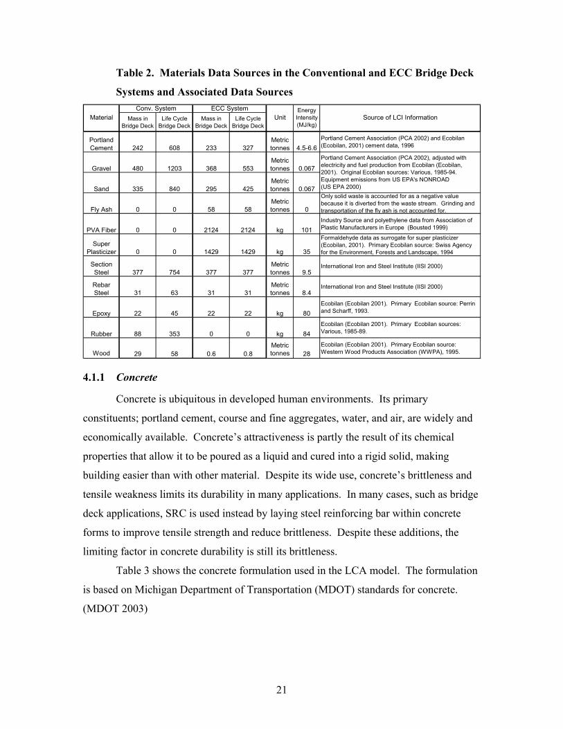
Table 2. Materials Data Sources in the Conventional and ECC Bridge Deck Systems and
Associated Data Sources........................................................................................... 21
Table 3. Conventional Concrete Formulation.................................................................. 22
Table 4. ECC Material Formulation ................................................................................ 22
Table 5. Kiln Configurations and Total Primary Energy per Kilogram of Cement
Produced ................................................................................................................... 25
Table 6. Volume of SRC, ECC, and Steel Required in Construction Processes ............. 27
Table 7. Equipment Usage During Construction Activities ............................................ 32
Table 8. NONROAD Output Categories Selected for LCA Model Use ......................... 33
Table 9. Model Limitations and Assumptions................................................................. 48
Table 10. Multi-Perspective Comparison of ECC and Conventional Concrete Material
Energy ....................................................................................................................... 49
Table 11. Life Cycle Raw Material Resource Use .......................................................... 50
Table 12. Kiln Configurations and Total Life Cycle Material Production Energy ......... 53

1 Introduction
1.1 Cement and its Significance
Our modern landscape cannot be characterized, described, or even imagined
without concrete materials. Concrete’s unique chemical properties that convert a
pourable liquid into a rigid and durable solid have defined the architecture and
infrastructure of our world. While cement is a material vital to human infrastructure and
economy, its production contributes a significant amount of carbon dioxide (CO2), a
greenhouse gas, to the atmosphere; approximately 5% of total anthropogenic emissions
(WBCSD 2002), and is one of the top two industry producers of CO2 (van Oss and
Padovani 2003). CO2 is produced both during the combustion of fuels for kiln heat, and
by the process of limestone calcination. Other important pollutants are produced during
the production process as well such as nitrogen oxides and sulfur dioxide emitted from
the cement kiln as a result of fuel combustion and heating of the material, and particulate
matter emitted from the cement kiln and during the cement milling process (USEPA
1999, CIF 2000). Environmental impacts associated with these pollutants pose risks to
human health and environmental and economic sustainability.
A holistic approach to evaluating and improving cement’s impact on the global
environment is needed to identify all the possible areas for improvement. Investment in
infrastructure is costly from both economic and material standpoints. Devising a
technique to predict long-term impacts of infrastructure design and material selection
could provide a strategic approach for reducing environmental impacts over time. In this
thesis a life cycle assessment (LCA) model is developed and applied to compare the
environmental impacts for a bridge containing conventional steel-reinforced concrete
joints, and an alternative design using link slabs constructed with a novel material –
Engineered Cementitious Composites (ECC).
2
1.2 LCA – A Holistic Approach
Life cycle assessment (LCA) is an analytical framework (ISO 1997) for
measuring environmental and social impacts of a product system or technology. LCA is
often described as a “cradle to grave” examination of a product or process, highlighting
environmental impacts and hidden costs that are often not reflected in conventional
assessments, which may focus on narrower boundaries and short-term issues. Cement
production, for example, requires a significant amount of energy to supply the high kiln
temperatures required to generate the chemical reactions that convert limestone into
clinker, the precursor to cement. This chemical reaction, or calcination, requires driving
CO2 out of the rock and into the atmosphere. Thus, the CO2 emitted during cement
production comes both from fuel combustion to run the kiln, as well as from the
calcination process that occurs in the kiln. However, the production process alone does
not account for the application, or use phase, of the cement product. Concrete materials
provide a valuable service in their applications in infrastructure. While production
impacts are important to recognize, so is the performance of the resultant material in the
field. Durability may prove to be more important from a life cycle perspective than the
impact of production, so a tradeoff between production impacts and performance during
application may have to be made. This thesis examines the application of cement as
applied in a concrete bridge deck. Cement, the binding agent in concrete, impacts the
bridge deck system based on its performance. For example, when the concrete bridge
deck cracks and repairs have to be made, traffic congestion results from the repair
process as traffic patterns are altered and road capacity is reduced. The additional fuel
used by these cars while they are delayed results in increased levels of CO2 emissions.
This fact highlights the need for a cradle-to-grave understanding of products and
materials. Without it, the true impacts of using a material may not be understood.
Despite the drawback of its production impacts, cement remains fundamental to
our modern infrastructure system and new, advanced cementitious materials are being
developed that promise longer life, improved mechanical properties, and perhaps reduced
life cycle emissions. Strategic application of these materials in new or existing structures
is hoped to extend the life of infrastructure and reduce repair and reconstruction burdens.
By building an LCA model for infrastructure applications that is able to compare
3
conventional cement materials and ECC over the entire life cycle of the infrastructure
application, an understanding of the potential benefits of these advanced ECC materials
will be gained.
The LCA methodology is applied to two alternative bridge deck designs and
evaluates the suitability of one design over another based on varying conditions specified
in the model. The model is designed to be flexible by allowing changes in most model
components, including bridge deck design, material selection, and traffic conditions.
1.3 Research Objectives
This project results from an interdisciplinary collaboration of researchers at the
University of Michigan. Researchers with expertise in Civil Engineering, Industrial
Ecology, Economics, and Economic Geology came together to explore the impacts and
potential future improvements of cement materials in modern infrastructure.
The research for this project was funded through the National Science Foundation
(NSF) with a Materials Use: Science, Engineering, and Society (MUSES) grant. The
objective of the MUSES program is to reduce “adverse human impact on the total,
interactive system of resource use, as well as maximizing the efficient use of individual
materials throughout their life cycles.” (NSF 2004) In order to reach the goals of
MUSES, an interdisciplinary group of researchers came together with a plan to integrate
macro-scale modeling, in this case an LCA model, and microstructure tailoring of novel
materials, ECC, in order to maximize the environmental benefits of material design over
the life cycle of its application. This thesis has two primary objectives:
1) The development of the LCA model
2) The application of the model to a bridge deck system.
By reaching these objectives, the model provides macro-scale modeling capability to the
research team.
4
1.4 Organization of this Report
This thesis is divided into seven sections. In this section a description of why
cement and its impacts are an important topic of study, the origin of the study, and the
need for a life cycle assessment approach are provided.
Section 2 provides a discussion of key background topics including, the system
definition, an in-depth description of LCA, the goals of LCA model development, and
previous research relevant to this study.
Section 3 focuses on LCA model development and highlights two key features of
model development; defining the functional unit and the bridge infrastructure life cycle
timeline used in the model.
Computer model development is discussed in Section 4. Computer model
architecture and its relationship to each major phase of the LCA model are described.
The logic sequence for each computer program module is outlined.
Section 5 describes the datasets used in the model and provides a summary of
model limitations and assumptions.
The final results of the model are provided in Section 6. Life cycle impacts
including raw material use, energy consumption, solid waste, air emissions, water
discharges, and green house gas emissions are presented for the ECC and conventional
systems.
Section 6 puts forward conclusions and recommendations for future research.
5
2 Background and Previous Work
2.1 Background
An estimated one-third of U.S. roadways are in poor or mediocre condition
(ASCE 2001), burdening the public with construction related impacts such as congestion
(TRIP 2002) and vehicle damage (ASCE 2001; TRIP 2002). Poor roadway conditions
have lead to continued material and economic investment in highways and roads of
approximately 260 million metric tons of concrete annually in the U.S. (Kelly 1998).
This figure illustrates the need to approach road building and repair from a new
perspective – long term and preventive, rather than short term and corrective. The life
cycle assessment (LCA) methodology provides the means for this kind of evaluation.
The LCA framework is designed to evaluate a product or process throughout its
life cycle, including raw material acquisition, production, use, final disposal or recycling,
and the transportation needed between these phases (ISO 1997). Often, LCA elucidates
unseen environmental and social burdens incurred over a product’s lifetime.
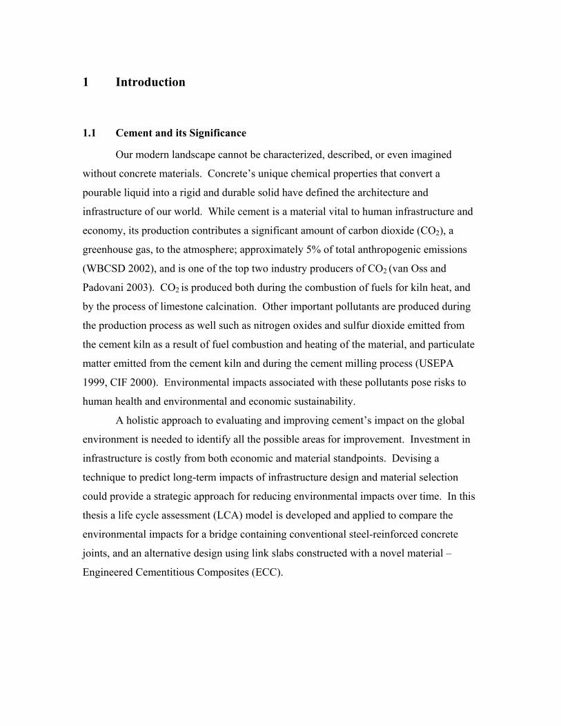
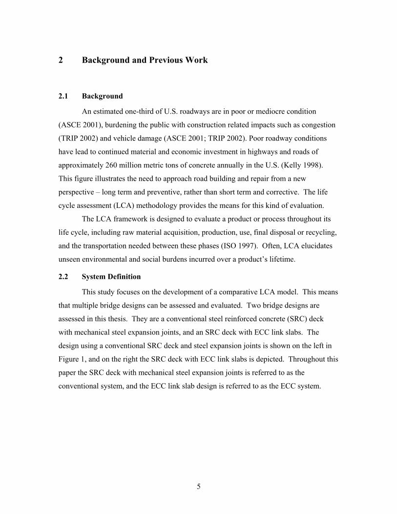
2.2 System Definition
This study focuses on the development of a comparative LCA model. This means
that multiple bridge designs can be assessed and evaluated. Two bridge designs are
assessed in this thesis. They are a conventional steel reinforced concrete (SRC) deck
with mechanical steel expansion joints, and an SRC deck with ECC link slabs. The
design using a conventional SRC deck and steel expansion joints is shown on the left in
Figure 1, and on the right the SRC deck with ECC link slabs is depicted. Throughout this
paper the SRC deck with mechanical steel expansion joints is referred to as the
conventional system, and the ECC link slab design is referred to as the ECC system.
6
Conventional SystemECC System
Figure 1. Bridge Deck with ECC Link Slab and Conventional Mechanical Steel Expansion Joint
The system boundary includes the impacts of the bridge design on its users. The
impact on bridge users is manifested in construction related traffic, which increases fuel
use and emissions, and also has broader economic impacts such as time lost to motorists
or shipment delays to business. The time horizon in this model is always bounded at 60-
years. This is an important assumption and will be discussed more fully in Section 3.
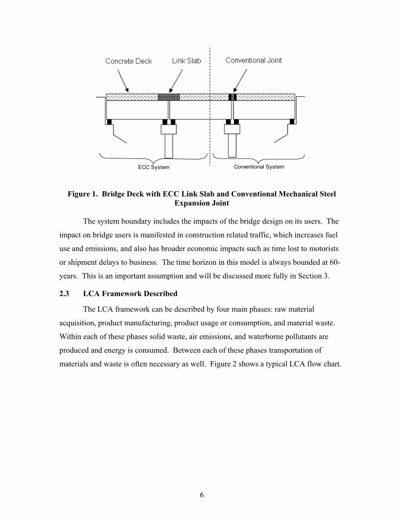
2.3 LCA Framework Described
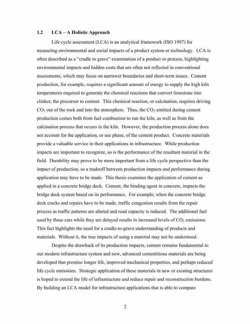
The LCA framework can be described by four main phases: raw material
acquisition, product manufacturing, product usage or consumption, and material waste.
Within each of these phases solid waste, air emissions, and waterborne pollutants are
produced and energy is consumed. Between each of these phases transportation of
materials and waste is often necessary as well. Figure 2 shows a typical LCA flow chart.
7
Manufacturing Use End-of-LifeRaw
Material Aquisition
d d d
d = distribution Recycling
Figure 2. Generic Life Cycle Framework Diagram
If we examine the plastic fiber used in ECC through its life cycle using the
diagram above, the raw material acquisition phase includes the drilling and refining of
petroleum to create the precursors to plastic. These products must be transported to the
manufacturing facility where they will be turned into plastic fibers. Manufacturing
requires energy and material inputs, such as electricity for the manufacturing plant and
process water used in manufacturing. The fibers must then be packaged and be
distributed to their final customer. In this case the final customer is the person mixing
and applying ECC. During its use-phase the ECC remains bound in the ECC matrix and
does not create any outputs or use any inputs. Finally, in the end-of-life phase the ECC
link slab is removed and trucked to a landfill. At this time there is no way to recycle the
plastic fibers entrained in the ECC, so the recycle loop shown above is not used. In
between phases where transport of the material occurs the fuel use, emissions from
combustion, and upstream burdens for fuel production need to be accounted for. This is
the life cycle of the plastic fiber, which is a single component in the life cycle of the
bridge deck system.
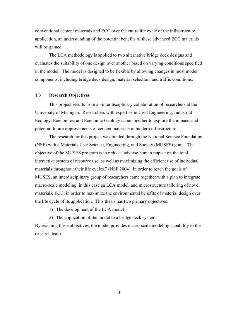
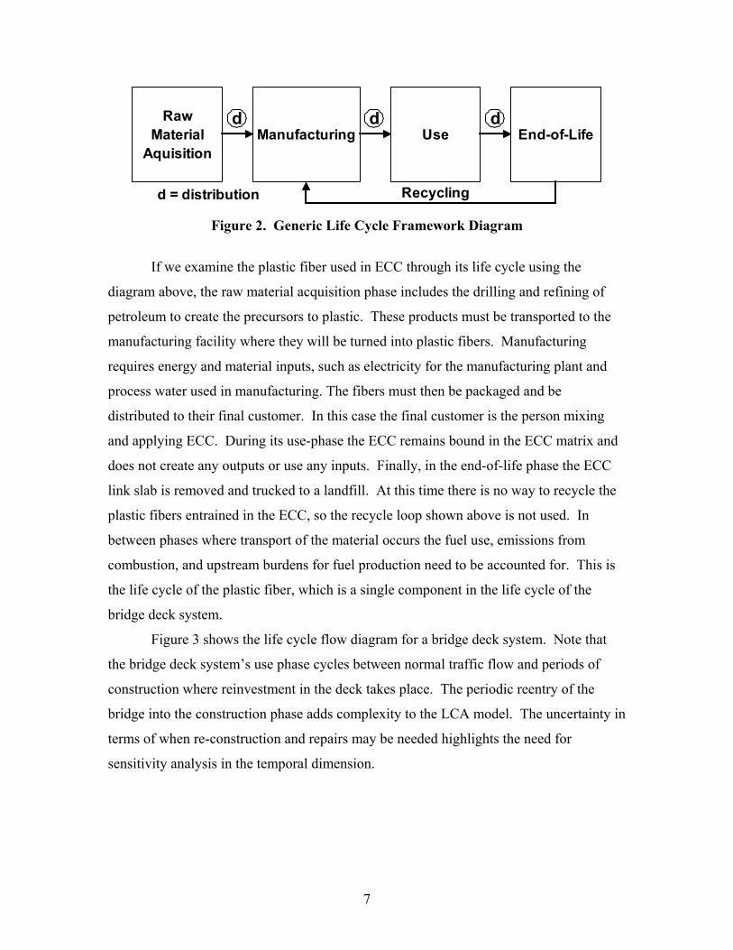
Figure 3 shows the life cycle flow diagram for a bridge deck system. Note that
the bridge deck system’s use phase cycles between normal traffic flow and periods of
construction where reinvestment in the deck takes place. The periodic reentry of the
bridge into the construction phase adds complexity to the LCA model. The uncertainty in
terms of when re-construction and repairs may be needed highlights the need for
sensitivity analysis in the temporal dimension.
8
d = distribution
Construction - Equipment Use
- Construction-related traffic congestion
- Fuel Use
Use- Vehicle traffic
- Fuel production
End-of-Life- Demolition
- Landfilling and Recycling
Material Production- Mining/extraction of
raw materials- Processing of raw
materials
Recycling
d d d
Bridge Repair
Figure 3. Bridge Deck System Life Cycle Framework Diagram
In modeling the framework described in Figure 3, each material and energy input
to the system requires a dataset that reflects the burdens and inputs associated with its
own life cycle, as outlined in Figure 2. For example, when modeling a bridge
construction event not only must the hours of operation and fuel economy of each piece
of equipment be defined to estimate fuel consumption, but also the life cycle data for the
diesel consumed by the machinery including upstream burdens (burdens associated with
petroleum extraction, refining, and transport) and the impacts of combustion such as the
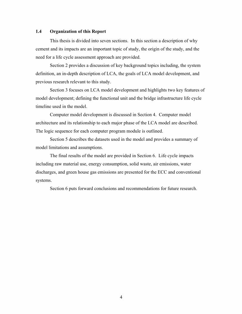
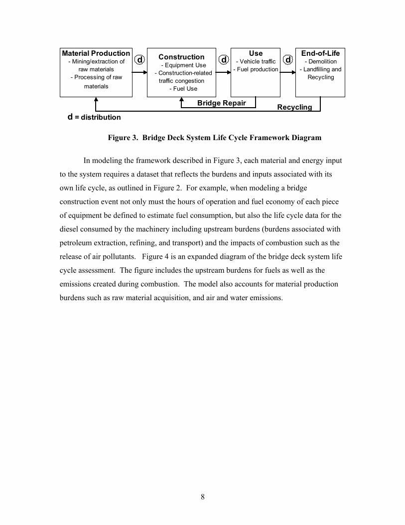
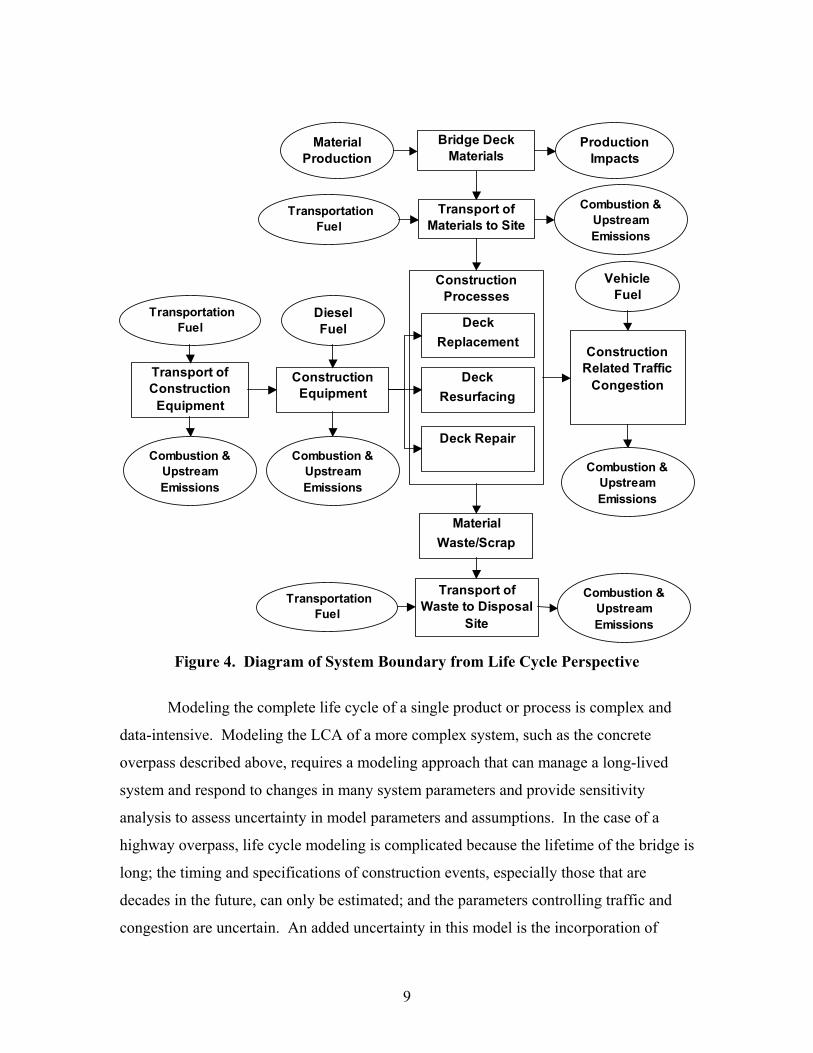
release of air pollutants. Figure 4 is an expanded diagram of the bridge deck system life
cycle assessment. The figure includes the upstream burdens for fuels as well as the
emissions created during combustion. The model also accounts for material production
burdens such as raw material acquisition, and air and water emissions.
9
Construction Processes
Deck Replacement
Deck Resurfacing
Deck Repair
Construction Equipment
Diesel Fuel
Construction Related Traffic
Congestion
Material Waste/Scrap
Vehicle Fuel
Transport ofConstruction
Equipment
Transportation Fuel
Transport ofMaterials to Site
Transportation Fuel
Bridge Deck Materials
Production Impacts
Material Production
Combustion & Upstream Emissions
Combustion & Upstream Emissions
Combustion & Upstream Emissions
Combustion & Upstream Emissions
Transport ofWaste to Disposal
Site
Transportation Fuel
Combustion & Upstream Emissions
Figure 4. Diagram of System Boundary from Life Cycle Perspective
Modeling the complete life cycle of a single product or process is complex and
data-intensive. Modeling the LCA of a more complex system, such as the concrete
overpass described above, requires a modeling approach that can manage a long-lived
system and respond to changes in many system parameters and provide sensitivity
analysis to assess uncertainty in model parameters and assumptions. In the case of a
highway overpass, life cycle modeling is complicated because the lifetime of the bridge is
long; the timing and specifications of construction events, especially those that are
decades in the future, can only be estimated; and the parameters controlling traffic and
congestion are uncertain. An added uncertainty in this model is the incorporation of
10
novel materials and designs. While the mechanical properties of these new materials are
well studied and understood, empirical evidence of their behavior over time is simply not
available.
2.4 Life Cycle Inventory
The first stage of the LCA is creating a life cycle inventory (LCI) for the system
modeled. The LCI consists of the aggregated life cycle data for all of the energy and
material inputs, and outputs from the product system. In this case, the LCI consists of the
total aggregation of data over the bridge’s 60-year life. This means each material, energy
source, and transport mode must have an LCI dataset that describes its upstream burdens.
Upstream burdens are those that accrue prior to the use phase, such as raw material
acquisition and manufacturing or processing of materials. The LCI datasets and their
details are discussed further in the Materials section, section 4.1.
2.5 Goals of LCA Model Development: An Integrated Life Cycle Design
Framework
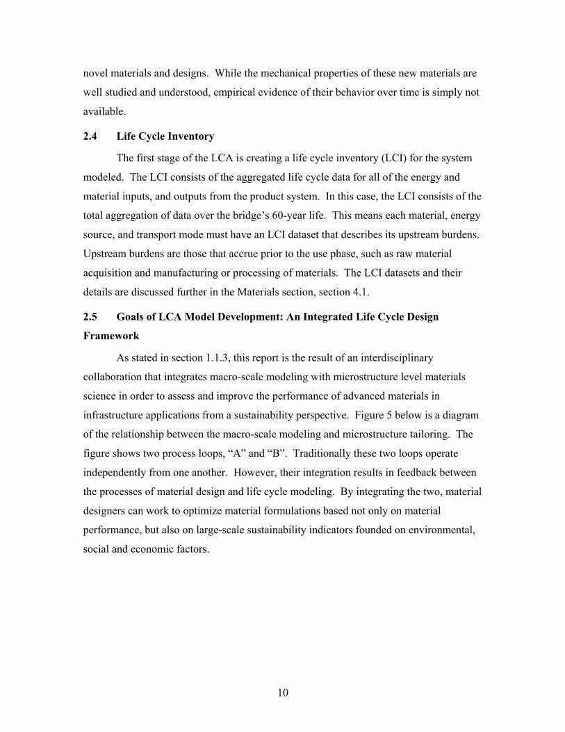
As stated in section 1.1.3, this report is the result of an interdisciplinary
collaboration that integrates macro-scale modeling with microstructure level materials
science in order to assess and improve the performance of advanced materials in
infrastructure applications from a sustainability perspective. Figure 5 below is a diagram
of the relationship between the macro-scale modeling and microstructure tailoring. The
figure shows two process loops, “A” and “B”. Traditionally these two loops operate
independently from one another. However, their integration results in feedback between
the processes of material design and life cycle modeling. By integrating the two, material
designers can work to optimize material formulations based not only on material
performance, but also on large-scale sustainability indicators founded on environmental,
social and economic factors.
11
Multi-scale Boundaries:• Microstructure ECC design• Macroscale life cycle analysis
Multi-criteria Sustainability Indicators:• Environmental• Social• Economic
Multi-project Infrastructure Applications:• Bridge decks• Roadways• Pipes
Multi-disciplinary Expertise:• Materials Science• Civil Engineering• Geology
• Industrial Ecology• Envir. Econ. & Policy• Envir. Health Sciences
Material
DesignIntegration
Input Materials & Composition
Microstructure Tailoring
ECC Physical Properties
Infrastructure Application
SustainabilityIndicatorsLife Cycle Modeling
PROCESS LOOP “A”
PROCESS LOOP “B”
Multi-scale Boundaries:• Microstructure ECC design• Macroscale life cycle analysis
Multi-criteria Sustainability Indicators:• Environmental• Social• Economic
Multi-project Infrastructure Applications:• Bridge decks• Roadways• Pipes
Multi-disciplinary Expertise:• Materials Science• Civil Engineering• Geology
• Industrial Ecology• Envir. Econ. & Policy• Envir. Health Sciences
Multi-disciplinary Expertise:• Materials Science• Civil Engineering• Geology
• Industrial Ecology• Envir. Econ. & Policy• Envir. Health Sciences
Material
DesignIntegration
Input Materials & Composition
Microstructure Tailoring
ECC Physical Properties
Infrastructure Application
SustainabilityIndicatorsLife Cycle Modeling
PROCESS LOOP “A”
PROCESS LOOP “B”
Material
DesignIntegration
Input Materials & Composition
Input Materials & Composition
Microstructure Tailoring
Microstructure Tailoring
ECC Physical Properties
ECC Physical Properties
Infrastructure Application
SustainabilityIndicatorsLife Cycle ModelingInfrastructure
ApplicationInfrastructure Application
SustainabilityIndicators
SustainabilityIndicatorsLife Cycle ModelingLife Cycle Modeling
PROCESS LOOP “A”
PROCESS LOOP “B”
Figure 5. Integrated Materials Design Framework for Sustainable Infrastructure
This thesis focuses on developing and quantifying the environmental
sustainability indicators in process loop “B”. Feedback from the LCA model provides
the material designers with information that helps move ECC formulations towards
“greenness”. Green formulations are those that substitute some of the more
environmentally and energy intensive materials with less intensive materials like
byproducts or wastes from other industrial processes. The idea is that through iterations
in material formulations and their associated LCA, an optimal formulation for ECC can
be developed that balances ECC link slab performance and the extent to which green
materials are incorporated in its formulation.
2.6 Previous Research
In the case of concrete bridges, only a limited number of LCA’s have been
performed and published. Horvath and Hendrickson (Horvath and Hendrickson 1998)
applied economic input-output life cycle assessment (EIO-LCA) to evaluate and compare
steel and steel reinforced concrete bridge girders. The EIO-LCA method traces economic
transactions throughout the supply chain of a product system and evaluates resource
requirements and environmental emissions using a commodity input-output model
12
coupled with key environmental impact datasets. Horvath and Hendrickson’s analysis
focused on material production, girder maintenance and end-of-life management
activities. They concluded that steel reinforced concrete girders were preferable to steel
girders, but the rate of recycling and incorporation of recycled steel in the girders could
affect these results.
In contrast, the model described in this paper employs process level LCA methods
to a more extensive system boundary that encompasses the interface between the material
elements of the bridge deck and the roadway’s users. The expanded system boundary
results in a more comprehensive environmental assessment for material selection. Of the
two bridge deck systems compared, the ECC link slab design is costlier from an initial
material and cost standpoint. However, greater initial investment may be merited from a
life cycle perspective.
While LCA methodology has rarely been applied to evaluate roadway systems,
key road building materials and their applications such as asphalt pavement (Franklin
Associates 2001) have been evaluated. Nevertheless environmental LCA is not often
incorporated in the decision making process of road building and repair. Life cycle
costing (LCC), however, has become increasingly important in transportation funding
and projects. (FHWA 1998) While LCC focuses on the life cycle costs of projects, its
growing role in transportation dialogues highlights that decision-makers have begun to
recognize the need for more holistic ways of thinking about investing in roads and
highways. This may signal a new paradigm in infrastructure planning that will be more
open to accepting environmental LCA as a decision-making tool.
A broader array of literature exists for LCC modeling of concrete bridges than for
LCA modeling. Previously developed life cycle costing methods, such as those
published by M. A. Ehlen include agency and user costs (driver delay, vehicle operating
and vehicle accident costs) and third party costs (Ehlen 1997). Ehlen classified third
party costs as the upstream environmental costs associated with construction materials
(pollution from mining, processing, and transportation) and the downstream
environmental costs related to construction activities such as runoff (Ehlen 1997). While
the increasing importance of third party costs were noted, they were not quantified and
environmental impacts from construction related traffic delay were not identified in
13
Ehlen’s LCC model. A more holistic approach was taken in a thesis by Richard Chandler
entitled “Life-Cycle Cost Model for Evaluating the Sustainability of Bridge Decks: A
comparison of conventional concrete joints and engineered cementitious composite link
slabs” (Chandler 2004). This thesis was based on results produced by an earlier version
of the LCA model described in this thesis. Chandler’s thesis was far-reaching in its
analysis, quantifying social, environmental, and user and agency costs. His results
showed that costs incurred by road users during congestion dominated all others. This
shows the need for improved integration of expanded life cycle costing methods that look
beyond conventional costing and examine social and environmental costs as well.
The key distinction between Chandler’s LCA model and the one described in this
thesis is his more frequent repair rate for both the ECC and conventional systems.
Chandler’s conclusions were unequivocal and, since the models are otherwise similar, are
suggestive of results expected for this LCA model.
14
3 Model Design and Framework
3.1 Model Structure
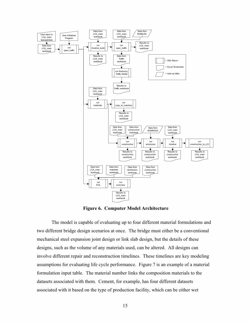
The LCA model is Microsoft Excel-based and runs six different workbooks using
12 Visual Basic Macros. Macros are programs written in Visual Basic (VBA) that are
run within Microsoft’s Excel software. The LCA_main workbook is the hub of the model
and provides and receives information from the five others; traffic, construction,
materials, distribution, and end-of-life. LCA_main houses the basic assumptions, the
majority of user-input requirements, the key command macros, and the final inventory
output for the entire model. The Figure 6 below shows the flow of command through the
macro hierarchy. The figure shows the order in which the VBA macros are run; when
data and information are retrieved from Excel spreadsheets and two look-up tables
containing MOBILE6.2 and NONROAD data, and which workbooks retain calculation
results:
15
run open_traffic
User Initializes Program
Data from LCA_main workbook
run timeline_build
run open_traffic
run materials
Data from LCA_main workbook
Data from LCA_main workbook
Results to LCA_main workbook
run Kentucky Traffic Model
Results to construction
workbook
Results to Traffic workbook
Data fromTraffic
workbook
run copy_to_inventory
Data from LCA_main workbook
Results to LCA_main workbook
run construction
Data from LCA_main workbook
Data from construction
workbook
run emissions
Data from NONROAD
Results to construction
workbook
run timeline
Data from LCA_main workbook
Results to construction
workbook
run construction_to_LCI
Results to LCA_main workbook
run EOL
Data from LCA_main workbook
Data from materials workbook
Data from distribution workbook
Data from construction
workbook
run summary
Results to LCA_main workbook
User Input to LCA_main
Spreadsheet
Data from MOBILE6.
2
Results to LCA_main workbook
= VBA Macro
= Excel Worksheet
= look-up table
Figure 6. Computer Model Architecture
The model is capable of evaluating up to four different material formulations and
two different bridge design scenarios at once. The bridge must either be a conventional
mechanical steel expansion joint design or link slab design, but the details of these
designs, such as the volume of any materials used, can be altered. All designs can
involve different repair and reconstruction timelines. These timelines are key modeling
assumptions for evaluating life cycle performance. Figure 7 is an example of a material
formulation input table. The material number links the composition materials to the
datasets associated with them. Cement, for example, has four different datasets
associated with it based on the type of production facility, which can be either wet
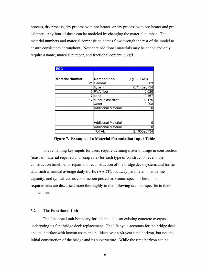
16
process, dry process, dry process with pre-heater, or dry process with pre-heater and pre-
calciner. Any four of these can be modeled by changing the material number. The
material numbers and material composition names flow through the rest of the model to
ensure consistency throughout. Note that additional materials may be added and only
require a name, material number, and fractional content in kg/L.
ECC
Material Number Composition (kg / L ECC)21 Cement 0.5834 fly ash 0.714398734
16 PVA fiber 0.0267 sand 0.467
17 super-plasticizer 0.0175water 0.298Additional Material 0
Additional Material 0Additional Material 0TOTAL 2.105898734
Figure 7. Example of a Material Formulation Input Table
The remaining key inputs for users require defining material usage in construction
(mass of material required and scrap rate) for each type of construction event, the
construction timeline for repair and reconstruction of the bridge deck system, and traffic
data such as annual average daily traffic (AADT), roadway parameters that define
capacity, and typical versus construction posted maximum speed. These input
requirements are discussed more thoroughly in the following sections specific to their
application.
3.2 The Functional Unit
The functional unit boundary for this model is an existing concrete overpass
undergoing its first bridge deck replacement. The life cycle accounts for the bridge deck
and its interface with human users and builders over a 60-year time horizon, but not the
initial construction of the bridge and its substructure. While the time horizon can be
17
varied in the LCA model, it is constrained by the difficulty of performing comparative
LCA on bridge deck systems with life times that do not share a common multiple within
a reasonable time horizon. For example, if the conventional system is expected to last 42
years, and the ECC system 60-years, the first year when both systems will complete a life
cycle and have no years of useful life remaining is at year 420. This time horizon is
clearly not reasonable for assessing infrastructure applications of this kind. While
choosing years of service such as 30 and 60 for the two systems cannot always be the
case in real-world applications, the model currently does not have the capability to
evaluate bridge deck systems whose life cycles are not equal or multiples of one another.
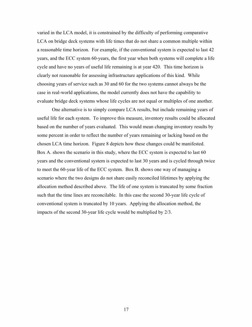
One alternative is to simply compare LCA results, but include remaining years of
useful life for each system. To improve this measure, inventory results could be allocated
based on the number of years evaluated. This would mean changing inventory results by
some percent in order to reflect the number of years remaining or lacking based on the
chosen LCA time horizon. Figure 8 depicts how these changes could be manifested.
Box A. shows the scenario in this study, where the ECC system is expected to last 60
years and the conventional system is expected to last 30 years and is cycled through twice
to meet the 60-year life of the ECC system. Box B. shows one way of managing a
scenario where the two designs do not share easily reconciled lifetimes by applying the
allocation method described above. The life of one system is truncated by some fraction
such that the time lines are reconcilable. In this case the second 30-year life cycle of
conventional system is truncated by 10 years. Applying the allocation method, the
impacts of the second 30-year life cycle would be multiplied by 2/3.
18
60 years
30 years
30 years
1 ECC Lifetime
2 Conventional Lifetimes
50 years
30 years
30 years
1 ECC Lifetime
2 Conventional Lifetimes
30 years
20 10 years
Burdens for 2nd 30-year lifetime truncated by 10 years
to match 50-year lifetime
50 years
1 ECC Lifetime
Box A.
Box B.
Figure 8. Alternatives for Managing Life Cycle Timelines
Drawing firm conclusions from the strategy shown in Figure 8, Box B may not be
straightforward. Thus, based on judgments from engineering, and for the purpose of
evaluation, the conventional deck was assumed to require replacement at 30 years, and
the ECC at 60, making comparison tenable.
The definition of the functional unit explicitly means that inputs and burdens
associated with the bridge’s substructure are outside the scope of this model, despite that
there are interactions between the deck and the substructure. Material inputs to the
bridge deck, inputs required for repair and reconstruction, traffic congestion caused by
construction events, and the distribution of inputs and waste from each of these elements
are included in the model. While traffic congestion is measured and reported, the traffic
that passes over the bridge on a daily basis is not directly reported in the model for three
primary reasons. The daily traffic is assumed to be the same regardless of the bridge
design selected, thus during non-construction periods in the use phase, the systems are
considered identical. Additionally, the fuel use by trucks and automobiles that pass over
19
the bridge everyday dwarf all the energy and air pollution associated with the other life
cycle phases so reporting these values obfuscates other phases and impacts in the life
cycle. The third and final reason is more philosophical than quantitative. The purpose of
the model is to measure the life cycle impact of a bridge design decision. Regardless of
the bridge design chosen, daily traffic will continue to pass over the bridge. Thus, the
design impact is independent of daily traffic flow except when the design impacts the
flow, such as during construction events. Thus, the appropriate way to represent the
impact of construction periods is to measure how it differs from normal periods of traffic
flow. Throughout the model and this thesis, traffic impacts refer to quantities as the
difference between construction period traffic flow and normal, or baseline, flow.
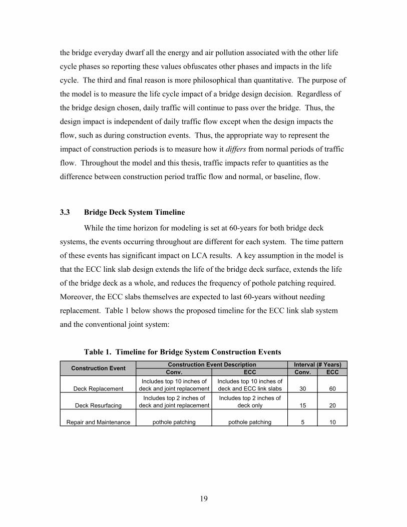
3.3 Bridge Deck System Timeline
While the time horizon for modeling is set at 60-years for both bridge deck
systems, the events occurring throughout are different for each system. The time pattern
of these events has significant impact on LCA results. A key assumption in the model is
that the ECC link slab design extends the life of the bridge deck surface, extends the life
of the bridge deck as a whole, and reduces the frequency of pothole patching required.
Moreover, the ECC slabs themselves are expected to last 60-years without needing
replacement. Table 1 below shows the proposed timeline for the ECC link slab system
and the conventional joint system:
Table 1. Timeline for Bridge System Construction Events
Conv. ECC Conv. ECC
Deck ReplacementIncludes top 10 inches of
deck and joint replacementIncludes top 10 inches of deck and ECC link slabs 30 60
Deck ResurfacingIncludes top 2 inches of
deck and joint replacementIncludes top 2 inches of
deck only 15 20
Repair and Maintenance pothole patching pothole patching 5 10
Construction Event Construction Event Description Interval (# Years)
20
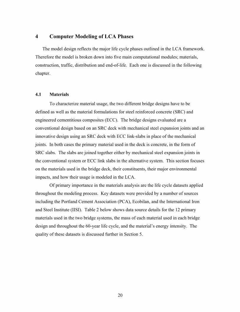
4 Computer Modeling of LCA Phases
The model design reflects the major life cycle phases outlined in the LCA framework.
Therefore the model is broken down into five main computational modules; materials,
construction, traffic, distribution and end-of-life. Each one is discussed in the following
chapter.
4.1 Materials
To characterize material usage, the two different bridge designs have to be
defined as well as the material formulations for steel reinforced concrete (SRC) and
engineered cementitious composites (ECC). The bridge designs evaluated are a
conventional design based on an SRC deck with mechanical steel expansion joints and an
innovative design using an SRC deck with ECC link-slabs in place of the mechanical
joints. In both cases the primary material used in the deck is concrete, in the form of
SRC slabs. The slabs are joined together either by mechanical steel expansion joints in
the conventional system or ECC link slabs in the alternative system. This section focuses
on the materials used in the bridge deck, their constituents, their major environmental
impacts, and how their usage is modeled in the LCA.
Of primary importance in the materials analysis are the life cycle datasets applied
throughout the modeling process. Key datasets were provided by a number of sources
including the Portland Cement Association (PCA), Ecobilan, and the International Iron
and Steel Institute (IISI). Table 2 below shows data source details for the 12 primary
materials used in the two bridge systems, the mass of each material used in each bridge
design and throughout the 60-year life cycle, and the material’s energy intensity. The
quality of these datasets is discussed further in Section 5.
21
Table 2. Materials Data Sources in the Conventional and ECC Bridge Deck
Systems and Associated Data Sources
Mass in Bridge Deck
Life Cycle Bridge Deck
Mass in Bridge Deck
Life Cycle Bridge Deck
Portland Cement 242 608 233 327
Metric tonnes 4.5-6.6
Portland Cement Association (PCA 2002) and Ecobilan (Ecobilan, 2001) cement data, 1996
Gravel 480 1203 368 553Metric tonnes 0.067
Sand 335 840 295 425Metric tonnes 0.067
Fly Ash 0 0 58 58Metric tonnes 0
Only solid waste is accounted for as a negative value because it is diverted from the waste stream. Grinding and transportation of the fly ash is not accounted for.
PVA Fiber 0 0 2124 2124 kg 101Industry Source and polyethylene data from Association of Plastic Manufacturers in Europe (Bousted 1999)
Super Plasticizer 0 0 1429 1429 kg 35
Formaldehyde data as surrogate for super plasticizer (Ecobilan, 2001). Primary Ecobilan source: Swiss Agency for the Environment, Forests and Landscape, 1994
Section Steel 377 754 377 377
Metric tonnes 9.5
International Iron and Steel Institute (IISI 2000)
Rebar Steel 31 63 31 31
Metric tonnes 8.4
International Iron and Steel Institute (IISI 2000)
Epoxy 22 45 22 22 kg 80Ecobilan (Ecobilan 2001). Primary Ecobilan source: Perrin and Scharff, 1993.
Rubber 88 353 0 0 kg 84Ecobilan (Ecobilan 2001). Primary Ecobilan sources: Various, 1985-89.
Wood 29 58 0.6 0.8Metric tonnes 28
Ecobilan (Ecobilan 2001). Primary Ecobilan source: Western Wood Products Association (WWPA), 1995.
MaterialConv. System ECC System
Portland Cement Association (PCA 2002), adjusted with electricity and fuel production from Ecobilan (Ecobilan, 2001). Original Ecobilan sources: Various, 1985-94. Equipment emissions from US EPA's NONROAD (US EPA 2000)
Source of LCI InformationUnitEnergy Intensity (MJ/kg)
4.1.1 Concrete
Concrete is ubiquitous in developed human environments. Its primary
constituents; portland cement, course and fine aggregates, water, and air, are widely and
economically available. Concrete’s attractiveness is partly the result of its chemical
properties that allow it to be poured as a liquid and cured into a rigid solid, making
building easier than with other material. Despite its wide use, concrete’s brittleness and
tensile weakness limits its durability in many applications. In many cases, such as bridge
deck applications, SRC is used instead by laying steel reinforcing bar within concrete
forms to improve tensile strength and reduce brittleness. Despite these additions, the
limiting factor in concrete durability is still its brittleness.
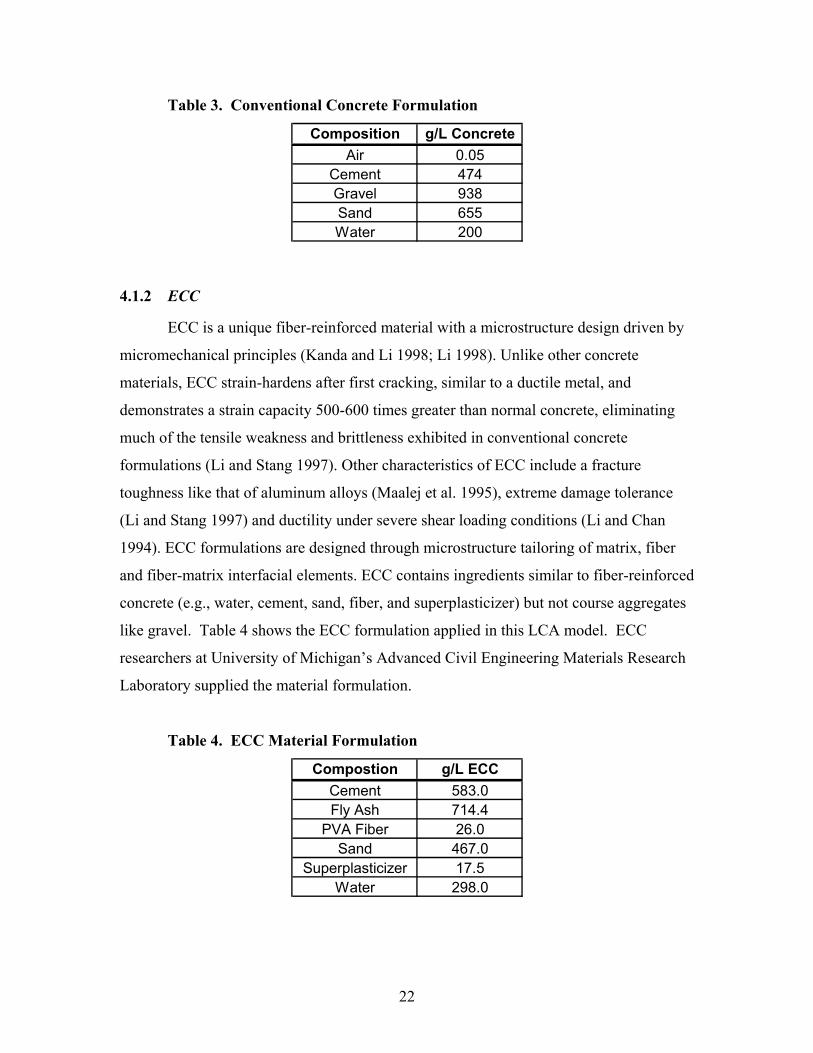
Table 3 shows the concrete formulation used in the LCA model. The formulation
is based on Michigan Department of Transportation (MDOT) standards for concrete.
(MDOT 2003)
22
Table 3. Conventional Concrete Formulation
Composition g/L ConcreteAir 0.05
Cement 474Gravel 938Sand 655Water 200
4.1.2 ECC
ECC is a unique fiber-reinforced material with a microstructure design driven by
micromechanical principles (Kanda and Li 1998; Li 1998). Unlike other concrete
materials, ECC strain-hardens after first cracking, similar to a ductile metal, and
demonstrates a strain capacity 500-600 times greater than normal concrete, eliminating
much of the tensile weakness and brittleness exhibited in conventional concrete
formulations (Li and Stang 1997). Other characteristics of ECC include a fracture
toughness like that of aluminum alloys (Maalej et al. 1995), extreme damage tolerance
(Li and Stang 1997) and ductility under severe shear loading conditions (Li and Chan
1994). ECC formulations are designed through microstructure tailoring of matrix, fiber
and fiber-matrix interfacial elements. ECC contains ingredients similar to fiber-reinforced
concrete (e.g., water, cement, sand, fiber, and superplasticizer) but not course aggregates
like gravel. Table 4 shows the ECC formulation applied in this LCA model. ECC
researchers at University of Michigan’s Advanced Civil Engineering Materials Research
Laboratory supplied the material formulation.
Table 4. ECC Material Formulation
Compostion g/L ECCCement 583.0Fly Ash 714.4
PVA Fiber 26.0Sand 467.0
Superplasticizer 17.5Water 298.0
23
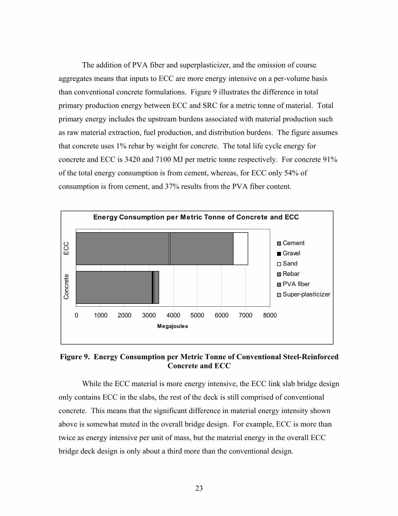
The addition of PVA fiber and superplasticizer, and the omission of course
aggregates means that inputs to ECC are more energy intensive on a per-volume basis
than conventional concrete formulations. Figure 9 illustrates the difference in total
primary production energy between ECC and SRC for a metric tonne of material. Total
primary energy includes the upstream burdens associated with material production such
as raw material extraction, fuel production, and distribution burdens. The figure assumes
that concrete uses 1% rebar by weight for concrete. The total life cycle energy for
concrete and ECC is 3420 and 7100 MJ per metric tonne respectively. For concrete 91%
of the total energy consumption is from cement, whereas, for ECC only 54% of
consumption is from cement, and 37% results from the PVA fiber content.
Energy Consumption per Metric Tonne of Concrete and ECC
0 1000 2000 3000 4000 5000 6000 7000 8000
Con
cret
eE
CC
Megajoules
CementGravelSandRebarPVA fiberSuper-plasticizer
Figure 9. Energy Consumption per Metric Tonne of Conventional Steel-Reinforced
Concrete and ECC
While the ECC material is more energy intensive, the ECC link slab bridge design
only contains ECC in the slabs, the rest of the deck is still comprised of conventional
concrete. This means that the significant difference in material energy intensity shown
above is somewhat muted in the overall bridge design. For example, ECC is more than
twice as energy intensive per unit of mass, but the material energy in the overall ECC
bridge deck design is only about a third more than the conventional design.
24
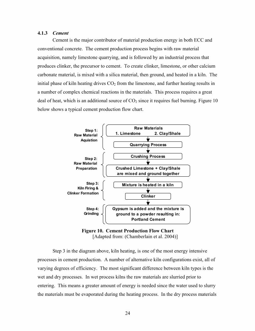
4.1.3 Cement Cement is the major contributor of material production energy in both ECC and
conventional concrete. The cement production process begins with raw material
acquisition, namely limestone quarrying, and is followed by an industrial process that
produces clinker, the precursor to cement. To create clinker, limestone, or other calcium
carbonate material, is mixed with a silica material, then ground, and heated in a kiln. The
initial phase of kiln heating drives CO2 from the limestone, and further heating results in
a number of complex chemical reactions in the materials. This process requires a great
deal of heat, which is an additional source of CO2 since it requires fuel burning. Figure 10
below shows a typical cement production flow chart.
Step 1: Raw Material
Aquistion
Step 2: Raw Material
Preparation
Step 3: Kiln Firing &
Clinker Formation
Step 4: Grinding
Raw Materials1. Limestone 2. Clay/Shale
Quarrying Process
Crushing Process
Crushed Limestone + Clay/Shale are mixed and ground together
Mixture is heated in a kiln
Clinker
Gypsum is added and the mixture is ground to a powder resulting in:
Portland Cement
Figure 10. Cement Production Flow Chart [Adapted from: (Chamberlain et al. 2004)]
Step 3 in the diagram above, kiln heating, is one of the most energy intensive
processes in cement production. A number of alternative kiln configurations exist, all of
varying degrees of efficiency. The most significant difference between kiln types is the
wet and dry processes. In wet process kilns the raw materials are slurried prior to
entering. This means a greater amount of energy is needed since the water used to slurry
the materials must be evaporated during the heating process. In the dry process materials
25
enter the kiln dry, and thus the kiln heat goes directly towards heating the raw material.
In general, wet process kilns only exist in older plants that have not yet been updated
with the improved dry process systems.
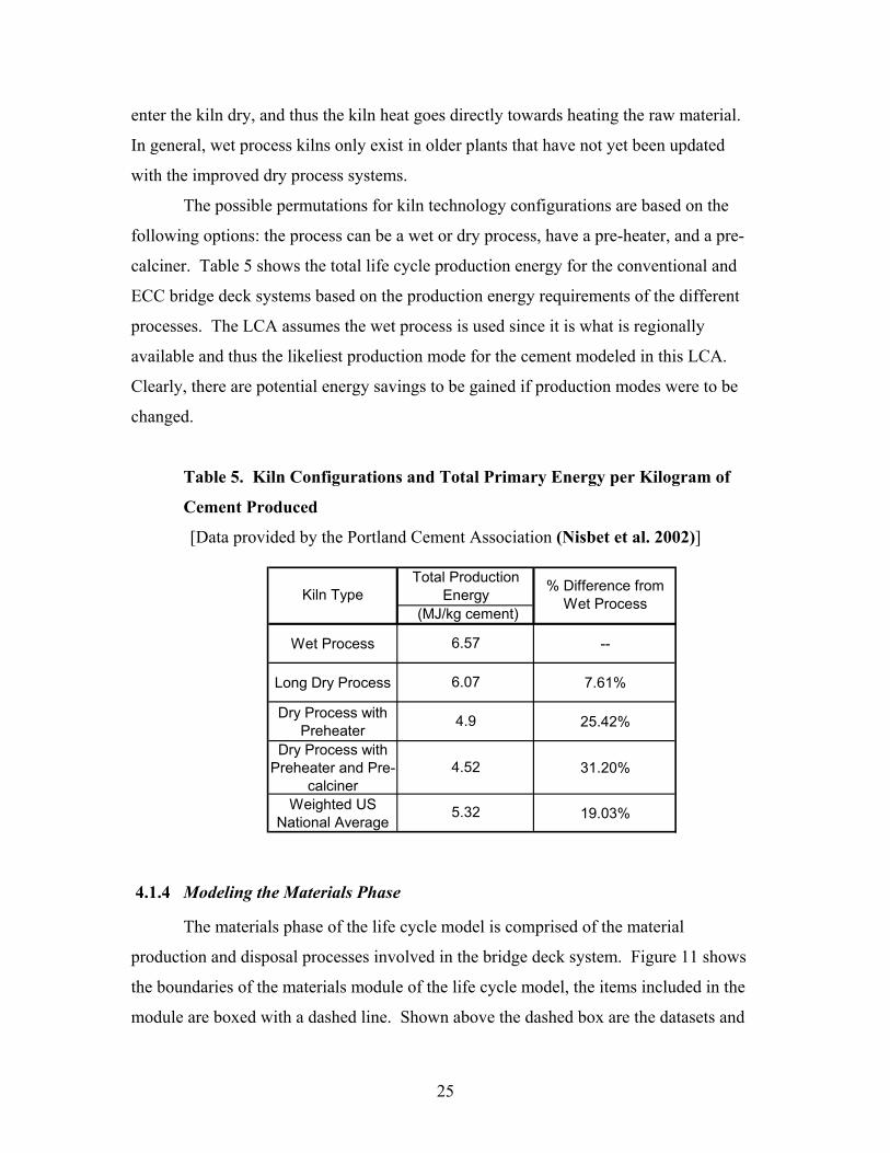
The possible permutations for kiln technology configurations are based on the
following options: the process can be a wet or dry process, have a pre-heater, and a pre-
calciner. Table 5 shows the total life cycle production energy for the conventional and
ECC bridge deck systems based on the production energy requirements of the different
processes. The LCA assumes the wet process is used since it is what is regionally
available and thus the likeliest production mode for the cement modeled in this LCA.
Clearly, there are potential energy savings to be gained if production modes were to be
changed.
Table 5. Kiln Configurations and Total Primary Energy per Kilogram of
Cement Produced
[Data provided by the Portland Cement Association (Nisbet et al. 2002)]
Wet Process --
Long Dry Process 7.61%
Dry Process with Preheater 25.42%
Dry Process with Preheater and Pre-
calciner31.20%
Weighted US National Average 19.03%
6.07
4.52
5.32
Kiln TypeTotal Production
Energy (MJ/kg cement)
% Difference from Wet Process
6.57
4.9
4.1.4 Modeling the Materials Phase
The materials phase of the life cycle model is comprised of the material
production and disposal processes involved in the bridge deck system. Figure 11 shows
the boundaries of the materials module of the life cycle model, the items included in the
module are boxed with a dashed line. Shown above the dashed box are the datasets and
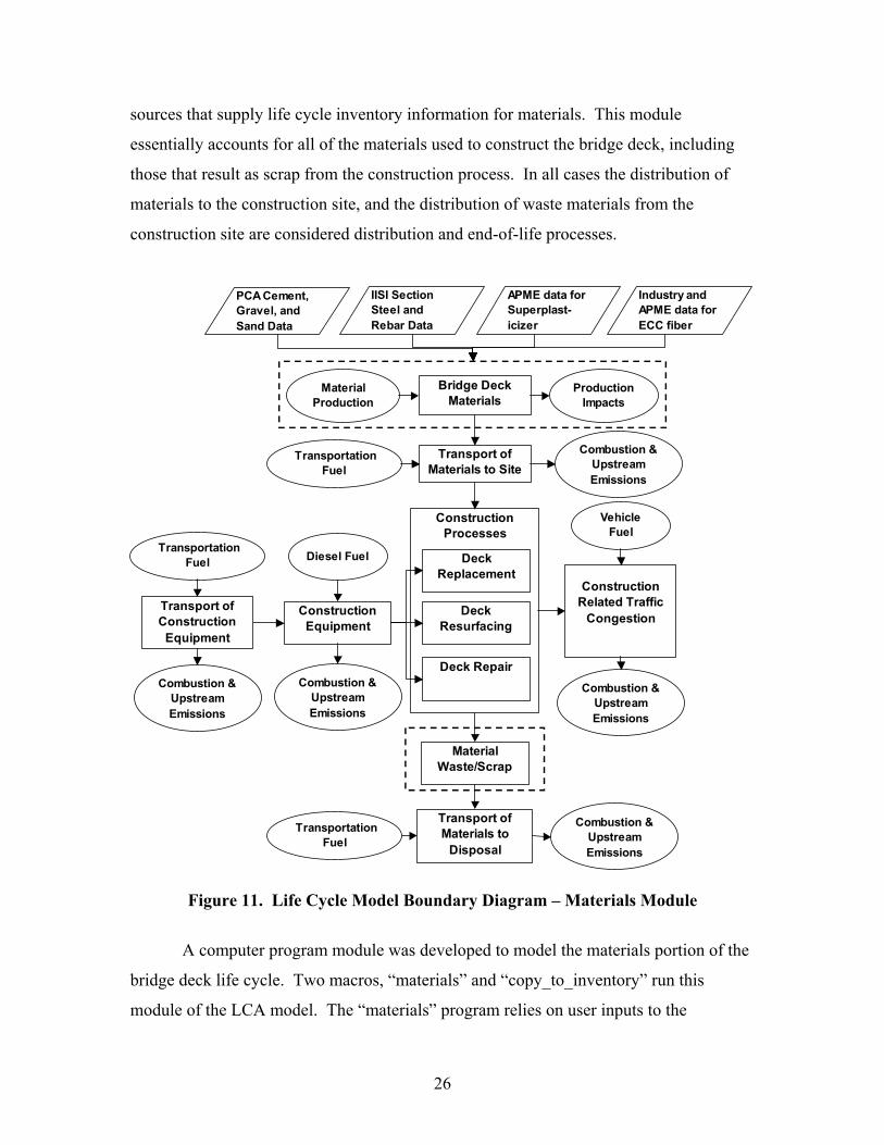
26
sources that supply life cycle inventory information for materials. This module
essentially accounts for all of the materials used to construct the bridge deck, including
those that result as scrap from the construction process. In all cases the distribution of
materials to the construction site, and the distribution of waste materials from the
construction site are considered distribution and end-of-life processes.
Transportation Fuel
Construction Processes
Deck Replacement
Deck Resurfacing
Deck Repair
Construction Equipment
Diesel Fuel
Construction Related Traffic
Congestion
Material Waste/Scrap
Bridge Deck Materials
Vehicle Fuel
Transport ofConstruction
Equipment
Production Impacts
Material Production
Transport ofMaterials to Site
Transportation Fuel
Transport ofMaterials to
Disposal
Transportation Fuel
PCA Cement, Gravel, and Sand Data
IISI Section Steel and Rebar Data
APME data for Superplast- icizer
Industry and APME data for ECC fiber
Combustion & Upstream Emissions
Combustion & Upstream Emissions
Combustion & Upstream Emissions
Combustion & Upstream Emissions
Combustion & Upstream Emissions
Figure 11. Life Cycle Model Boundary Diagram – Materials Module
A computer program module was developed to model the materials portion of the
bridge deck life cycle. Two macros, “materials” and “copy_to_inventory” run this
module of the LCA model. The “materials” program relies on user inputs to the
27
LCA_main spreadsheet defining bridge deck volume, the volume of steel expansion joints
or link slabs, construction scrap rate, and the timeline for repair and reconstruction. The
timeline is a key determinant of the bridge deck system’s life cycle performance.
Timeline specifications were developed based on information provided by participating
engineers, MDOT, and construction contractors.
As shown in Figure 11, there are three construction events that occur over the life
cycle of the bridge deck: deck replacement, deck resurfacing, and repair and
maintenance. The first two construction events are different in the link slab and
conventional systems. In the case of the ECC link slab system, a deck replacement
includes installation of link slabs to a depth of 11 inches and SRC deck replacement to a
depth of 10 inches. For a conventional joint system, deck replacement includes
installation of new joints surrounded with a concrete depth of 11 inches and deck
replacement to a depth of 10 inches. Table 6 below shows the different volumes of key
materials used in these construction events. A detailed inventory of material demands for
each type of construction event is also available in Appendix A. Additional materials are
needed for construction that are not part of the volumes shown here, such as wood used
in making concrete forms. The usage of additional materials is also included in
Appendix A.
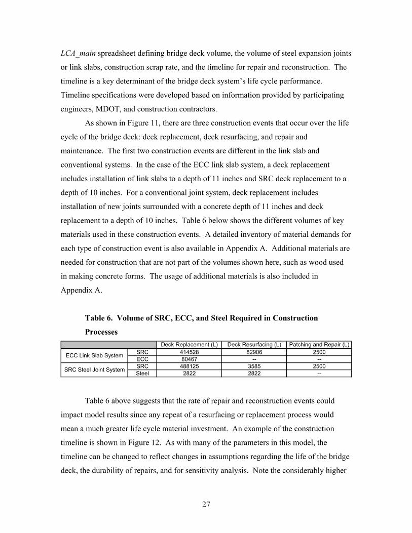
Table 6. Volume of SRC, ECC, and Steel Required in Construction
Processes Deck Replacement (L) Deck Resurfacing (L) Patching and Repair (L)
SRC 414528 82906 2500ECC 80467 -- --SRC 488125 3585 2500Steel 2822 2822 --
ECC Link Slab System
SRC Steel Joint System
Table 6 above suggests that the rate of repair and reconstruction events could
impact model results since any repeat of a resurfacing or replacement process would
mean a much greater life cycle material investment. An example of the construction
timeline is shown in Figure 12. As with many of the parameters in this model, the
timeline can be changed to reflect changes in assumptions regarding the life of the bridge
deck, the durability of repairs, and for sensitivity analysis. Note the considerably higher
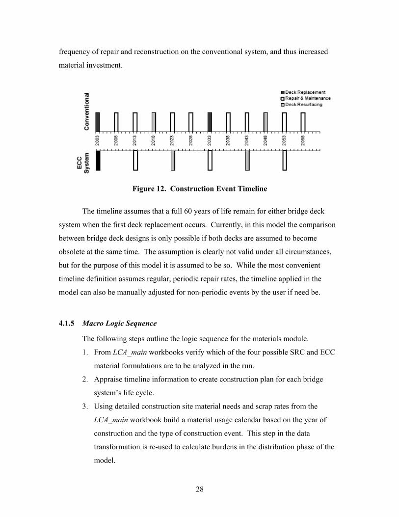
28
frequency of repair and reconstruction on the conventional system, and thus increased
material investment.
Figure 12. Construction Event Timeline
The timeline assumes that a full 60 years of life remain for either bridge deck
system when the first deck replacement occurs. Currently, in this model the comparison
between bridge deck designs is only possible if both decks are assumed to become
obsolete at the same time. The assumption is clearly not valid under all circumstances,
but for the purpose of this model it is assumed to be so. While the most convenient
timeline definition assumes regular, periodic repair rates, the timeline applied in the
model can also be manually adjusted for non-periodic events by the user if need be.
4.1.5 Macro Logic Sequence
The following steps outline the logic sequence for the materials module.
1. From LCA_main workbooks verify which of the four possible SRC and ECC
material formulations are to be analyzed in the run.
2. Appraise timeline information to create construction plan for each bridge
system’s life cycle.
3. Using detailed construction site material needs and scrap rates from the
LCA_main workbook build a material usage calendar based on the year of
construction and the type of construction event. This step in the data
transformation is re-used to calculate burdens in the distribution phase of the
model.
29
4. Create an output spreadsheet that multiplies inventory datasets by total mass
of each of the different materials used in a given year.
5. Export data from Materials workbook to LCA_main “Life_Cycle_Flows”
worksheets.
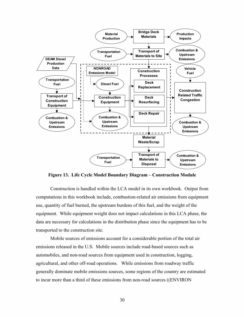
4.2 Construction
The construction module for the LCA model is significantly more complex than
the materials module. The construction process has two major environmental impacts
beyond material use and disposal, namely construction equipment use and traffic
congestion caused by the construction zone. The traffic congestion is dealt with in the
traffic module. The area boxed in with a dashed line in Figure 13 delineates the life cycle
model concepts that are included in the construction module.
30
Construction Processes
Deck Replacement
Deck Resurfacing
Deck Repair
Construction Equipment
Construction Related Traffic
Congestion
Material Waste/Scrap
Bridge Deck Materials
Vehicle Fuel
Transport ofConstruction
Equipment
Transportation Fuel
Production Impacts
Material Production
Transport ofMaterials to Site
TransportationFuel
Transport ofMaterials to
Disposal
TransportationFuel
NONROAD Emissions Model
Diesel Fuel
DEAM Diesel Production
Data
Combustion & Upstream Emissions
Combustion & Upstream Emissions
Combustion & Upstream Emissions
Combustion & Upstream Emissions
Combustion & Upstream Emissions
Figure 13. Life Cycle Model Boundary Diagram – Construction Module
Construction is handled within the LCA model in its own workbook. Output from
computations in this workbook include, combustion-related air emissions from equipment
use, quantity of fuel burned, the upstream burdens of this fuel, and the weight of the
equipment. While equipment weight does not impact calculations in this LCA phase, the
data are necessary for calculations in the distribution phase since the equipment has to be
transported to the construction site.
Mobile sources of emissions account for a considerable portion of the total air
emissions released in the U.S. Mobile sources include road-based sources such as
automobiles, and non-road sources from equipment used in construction, logging,
agricultural, and other off-road operations. While emissions from roadway traffic
generally dominate mobile emissions sources, some regions of the country are estimated
to incur more than a third of these emissions from non-road sources ((ENVIRON
31
International Corporation 2002); thus, modeling non-road emissions is essential in
estimating the total impacts of bridge design and material choice.
The US Environmental Protection Agency’s (EPA) NONROAD model was
selected as a tool to estimate fuel use and emissions from construction equipment based
on vehicle class and horsepower rating. NONROAD is still in its draft phase, and as such
cannot be considered with the full weight of confidence that goes with an approved EPA
model. Nevertheless, the NONROAD model is the most advanced tool available for this
type of calculation.
NONROAD is driven by a core program that runs in FORTRAN and a user
interface that runs in Visual Basic. While numerous input factors can be selected for
deriving output data, the data used for this LCA model was calculated based on the
region of use and selected by machine type defined by an equipment code and
horsepower class.
Construction activities are broken between end-of-life (EOL) and construction
processes. Those processes that involve demolishing and dismantling of bridge
components and removal of demolished materials from the construction site are
designated as EOL. All others are processes are designated as construction. In the final
LCA model results, the burdens associated with EOL processes from this phase are
presented as EOL, rather than construction. Since traffic controls are set-up and removed
only once from the construction site during any event, the initial traffic control set-up is
allocated to EOL because EOL is the first step in reconstruction events, and the removal
of traffic controls are allocated to construction.
Table 7 shows the construction machinery requirements for construction events
associated with the conventional joint and ECC link slab bridge designs. These
equipment requirements are based on estimates from a Michigan-based highway
contractor. The model is flexible with regard to equipment needs. Additional machinery
requirements for an event can be added and current ones can be altered or deleted and in
all cases estimated hours and days of usage can be changed.
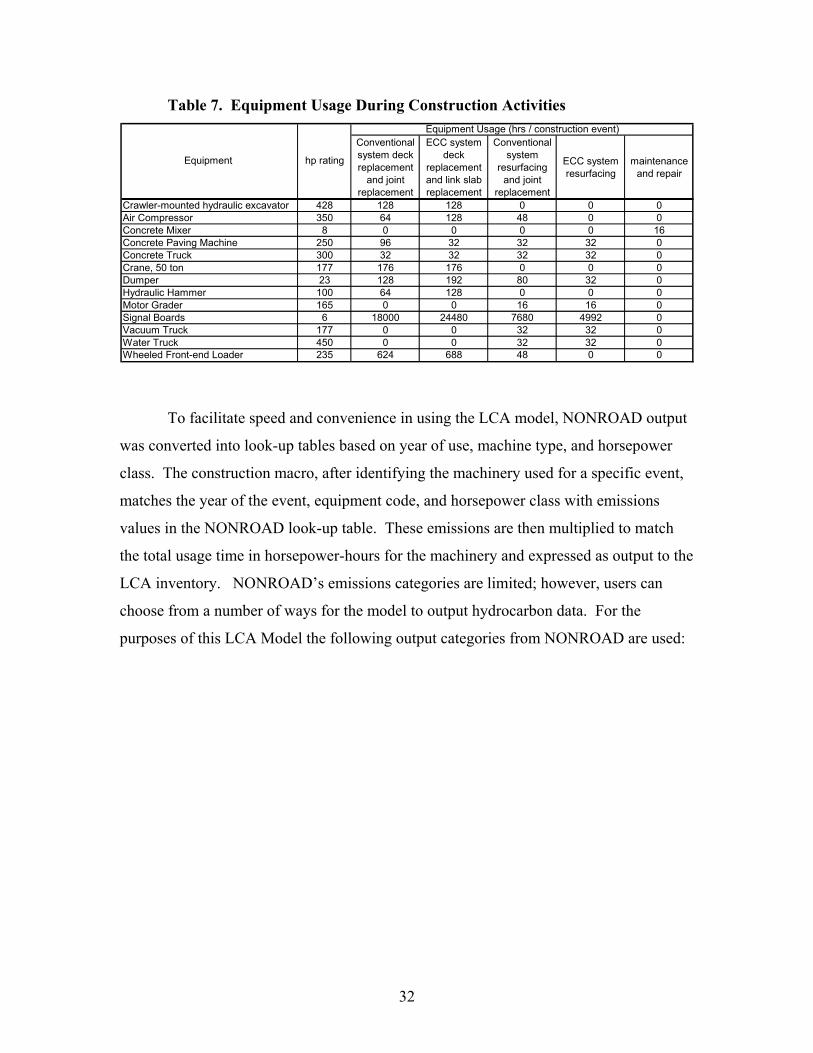
32
Table 7. Equipment Usage During Construction Activities
Conventional system deck replacement
and joint replacement
ECC system deck
replacement and link slab replacement
Conventional system
resurfacing and joint
replacement
ECC system resurfacing
maintenance and repair
Crawler-mounted hydraulic excavator 428 128 128 0 0 0Air Compressor 350 64 128 48 0 0Concrete Mixer 8 0 0 0 0 16Concrete Paving Machine 250 96 32 32 32 0Concrete Truck 300 32 32 32 32 0Crane, 50 ton 177 176 176 0 0 0Dumper 23 128 192 80 32 0Hydraulic Hammer 100 64 128 0 0 0Motor Grader 165 0 0 16 16 0Signal Boards 6 18000 24480 7680 4992 0Vacuum Truck 177 0 0 32 32 0Water Truck 450 0 0 32 32 0Wheeled Front-end Loader 235 624 688 48 0 0
Equipment Usage (hrs / construction event)
hp ratingEquipment
To facilitate speed and convenience in using the LCA model, NONROAD output
was converted into look-up tables based on year of use, machine type, and horsepower
class. The construction macro, after identifying the machinery used for a specific event,
matches the year of the event, equipment code, and horsepower class with emissions
values in the NONROAD look-up table. These emissions are then multiplied to match
the total usage time in horsepower-hours for the machinery and expressed as output to the
LCA inventory. NONROAD’s emissions categories are limited; however, users can
choose from a number of ways for the model to output hydrocarbon data. For the
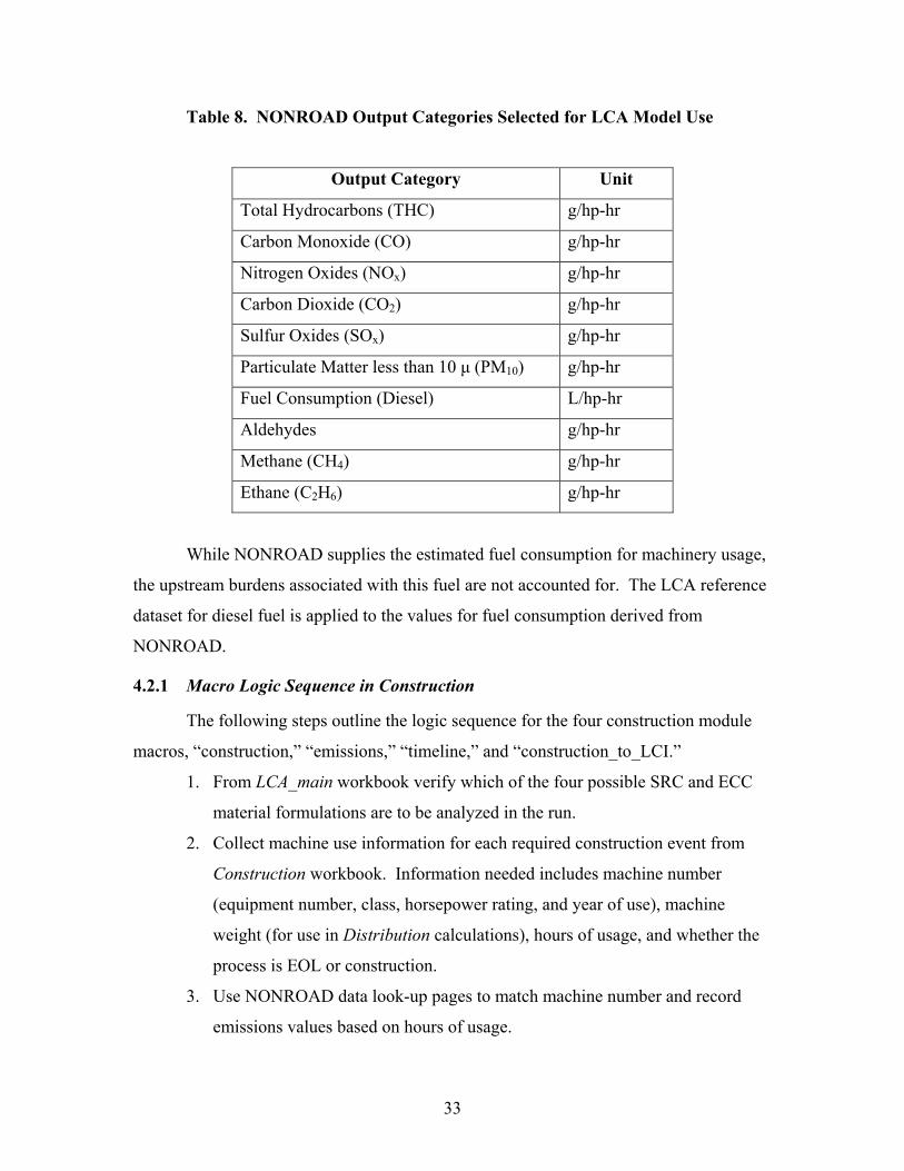
purposes of this LCA Model the following output categories from NONROAD are used:
33
Table 8. NONROAD Output Categories Selected for LCA Model Use
Output Category Unit
Total Hydrocarbons (THC) g/hp-hr
Carbon Monoxide (CO) g/hp-hr
Nitrogen Oxides (NOx) g/hp-hr
Carbon Dioxide (CO2) g/hp-hr
Sulfur Oxides (SOx) g/hp-hr
Particulate Matter less than 10 µ (PM10) g/hp-hr
Fuel Consumption (Diesel) L/hp-hr
Aldehydes g/hp-hr
Methane (CH4) g/hp-hr
Ethane (C2H6) g/hp-hr
While NONROAD supplies the estimated fuel consumption for machinery usage,
the upstream burdens associated with this fuel are not accounted for. The LCA reference
dataset for diesel fuel is applied to the values for fuel consumption derived from
NONROAD.
4.2.1 Macro Logic Sequence in Construction
The following steps outline the logic sequence for the four construction module
macros, “construction,” “emissions,” “timeline,” and “construction_to_LCI.”
1. From LCA_main workbook verify which of the four possible SRC and ECC
material formulations are to be analyzed in the run.
2. Collect machine use information for each required construction event from
Construction workbook. Information needed includes machine number
(equipment number, class, horsepower rating, and year of use), machine
weight (for use in Distribution calculations), hours of usage, and whether the
process is EOL or construction.
3. Use NONROAD data look-up pages to match machine number and record
emissions values based on hours of usage.
34
4. Copy and reformat results from Construction workbook into LCA_main
inventory worksheets based on sub-processes within each type of construction
event to ensure that construction output data can be allocated between EOL
and construction burdens.
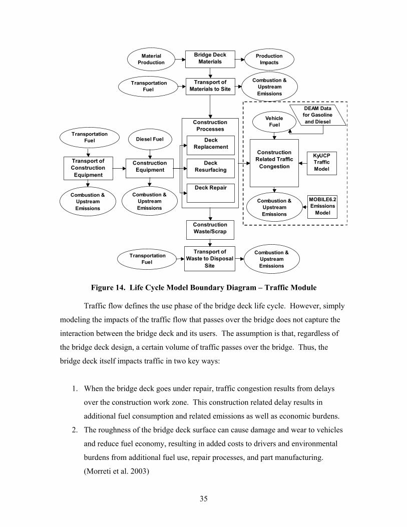
4.3 Traffic
The traffic phase of the life cycle analysis focuses only on traffic related to
construction processes. The dashed-line box in Figure 14 shows the portion of life cycle
modeling that is calculated in the traffic module. There are two important features of this
module evident in the figure below. The first is that only traffic disturbances caused by
construction events are accounted for in the model. These changes in traffic flow and
congestion are modeled using the KyUCP traffic model (Rister and Graves 2002). The
second important feature is the EPA’s MOBILE6.2 model, used in this section to
calculate combustion related emissions from traffic (USEPA 2002). MOBILE6.2 does
not calculate vehicle fuel use; thus, the LCA model calculates fuel consumption based on
speed of travel, vehicle type, and age for the fleet of vehicles on the road. Fuel economy
figures are based on estimates from the US EPA (Hellman and Heavenrich 2003).
35
Transport ofConstruction
Equipment
Transportation Fuel
Construction Processes
Deck Replacement
Deck Resurfacing
Deck Repair
Construction Equipment
Diesel Fuel
Construction Waste/Scrap
Transport ofMaterials to Site
Transportation Fuel
Transport ofWaste to Disposal
Site
Transportation Fuel
Bridge Deck Materials
Production Impacts
Material Production
MOBILE6.2 Emissions
Model
KyUCP Traffic Model
Construction Related Traffic
Congestion
Combustion & Upstream Emissions
Combustion & Upstream Emissions
Combustion & Upstream Emissions
Combustion & Upstream Emissions
Combustion & Upstream Emissions
DEAM Data for Gasoline and Diesel Vehicle
Fuel
Figure 14. Life Cycle Model Boundary Diagram – Traffic Module
Traffic flow defines the use phase of the bridge deck life cycle. However, simply
modeling the impacts of the traffic flow that passes over the bridge does not capture the
interaction between the bridge deck and its users. The assumption is that, regardless of
the bridge deck design, a certain volume of traffic passes over the bridge. Thus, the
bridge deck itself impacts traffic in two key ways:
1. When the bridge deck goes under repair, traffic congestion results from delays
over the construction work zone. This construction related delay results in
additional fuel consumption and related emissions as well as economic burdens.
2. The roughness of the bridge deck surface can cause damage and wear to vehicles
and reduce fuel economy, resulting in added costs to drivers and environmental
burdens from additional fuel use, repair processes, and part manufacturing.
(Morreti et al. 2003)
36
The second impact mentioned above cannot be feasibly modeled. While there is
clear evidence that rough surfaces and potholes cause significant wear and tear to
vehicles, quantifying the environmental impact is currently not possible. However, the
first impact, delays related to construction, can be modeled. Comparing the modeled
congestions to flow during non-construction (baseline) conditions, results in a value for
the impact of construction activities on traffic flow. This difference is in effect the
interaction between the bridge deck surface and vehicle traffic.
4.3.1 Traffic Model Selection
Traffic model selection is a key factor in this LCA since the use phase is highly
dependent on traffic model output for calculating the burdens associated with this phase.
A number of traffic models exist for modeling construction-related traffic delays,
including QUEWZ98 developed at the Texas Transportation Institute, CO3 developed by
Robert Carr at the University of Michigan, QuickZone developed at the Federal Highway
Administration (FHWA), and the Kentucky User Cost Program version 1.0 (KyUCP)
developed at University of Kentucky’s Kentucky Transportation Center. (Rister and
Graves 2002) Each of these models had exceptional strengths. For example, the
QUEWZ98 allows detailed detour routes to be included. However, in addition to
demanding a lot of user input, this model runs in DOS and outputs in DOS, meaning that
integration into the Excel-based LCA model proved difficult. Another model, CO3, also
proved difficult to integrate into this model as it is geared towards optimization of
construction cost and construction congestion (Carr 2000). Final model selection was
based on optimizing between the level of detail and traffic data demands, and the ease
with which the model could be integrated within the LCA. The KyUCP model was
chosen based on this selection criteria. This model, built from the DP-115 framework
developed by the FHWA, is an Excel-based model that outputs user delay data and user
cost data. Only the user delay output is incorporated into the LCA model.
DP-115 is the FHWA’s Demonstration Project No.115, Probabilistic LCCA in
Pavement Design (DP-115). The goal of this project was to develop recommended life
cycle cost assessment procedures for the national highway system (Walls and Smith
1998). In their September 1998 Technical Bulletin, the FHWA laid out the framework
37
and calculations for the DP-115 demonstration model. The KyUCP model was
developed from this framework, but incorporated the additional element of short-term
versus long-term construction sites. One attractive feature of this model is the limited
user input required; work zone capacity, work zone length, traffic flow rate based on
either annual average daily traffic (AADT) or hourly traffic data, normal highway
capacity, and percent of trucks on the road. Capacity calculations are based on the
Transportation Research Board’s Highway Capacity Manual (TRB 2000). Roadway
capacity changes during construction events because lanes are shut down necessitating
merges, speed is reduced, and because lane width may be reduced in the work zone. In
the LCA scenario modeled, capacity reduction during construction resulted from lane
shutdown and reduced speed, and normal highway capacity was correlated to lane width
and speed limit.
4.3.2 Vehicle Emissions
Once vehicle delay and congestion due to construction are calculated, these
results have to be coupled with fuel consumption and vehicle emissions data in order to
measure environmental impact. The US EPA’s MOBILE6.2 software was selected to
compute estimates of vehicle emissions. (USEPA 2002) MOBILE6.2 takes climatic,
temporal, and regional vehicle fleet data into consideration when estimating vehicle
emissions at various speeds. Predictions are available from the MOBILE6.2 software on
a per year basis through 2050. For years following 2050, the 2050 emission estimates are
used. MOBILE6.2 requires inputs regarding the geographic region where the vehicles
are driving. The geographic location, climate, and traffic flow for the bridge evaluated in
this LCA model are based on an overpass in Washtenaw County, Michigan at the
intersection of M-14 and US-23. The parameters provided for this bridge site include
annual average daily traffic (AADT) flow, and climatic conditions (necessary for
estimates in MOBILE6.2).
MOBILE6.2 output was recorded in look-up tables to facilitate speed and user
friendliness of the LCA model. If the location of the modeled bridge changes, the
MOBILE6.2 lookup tables would have to be updated to reflect this change.
MOBILE6.2 does not calculate carbon dioxide (CO2) emissions or fuel
consumption. This is a major shortcoming in the model given the magnitude of CO2
38
emitted from automobiles and the growing concern over its role in global warming. In
the LCA model an alternative mechanism for calculating these effects of construction
related traffic congestion was devised.
4.3.3 Fuel Consumption and Carbon Dioxide
In addition to direct emissions from vehicles, the amount of excess fuel consumed
as a result of delays was also calculated and the production and combustion of this fuel
was accounted for. Fuel consumption for cars and trucks was determined based on city
and highway drive cycle estimates of fuel economy. Data for cars came from US EPA
fuel economy data (Hellman and Heavenrich 2003) and commercial truck data from The
Technology Roadmap for the 21st Century Truck Program (Bradley 2000). A city drive
cycle is the closest estimate of fuel economy available for modeling the stop-and-go
movement typical of congestion. Likewise, a highway drive cycle for normal traffic flow
is used to model flow during non-construction and non-congestion periods. The final
results are calculated by subtracting emissions and fuel consumption during an equivalent
non-construction period from the results of a construction period. The construction
period results are the sum of the results from vehicles passing through the work zone
length, queue length, and detour length. These values are based on the total vehicle miles
traveled (VMT) at certain speeds.
The values for highway speed, highway capacity, work zone length, work zone
capacity, work zone speed, and AADT can all be changed in the LCA model. The
numbers used in this thesis are based on the real-world values associated with the
selected overpass, which defines AADT at approximately 70,000, with two lanes in each
direction, and a speed limit at 70 mph. (MDOT 1997). The work zone consists of one
lane in each direction, and a speed of 40 mph.
Drivers are expected to self-detour under many delay conditions. That is, even
when formal detour routes may not be used, many drivers will choose alternative routes if
back up is expected. While some congestion models have the capacity to account for this
behavior, the KyUCP model does not. In order to evaluate the importance of vehicle
detouring, the LCA model can modify input values to the KyUCP model to account for
detouring. The model is capable of computing up to three possible detour lengths, each
at different speeds with different percents of vehicles on each detour. Sensitivity analysis
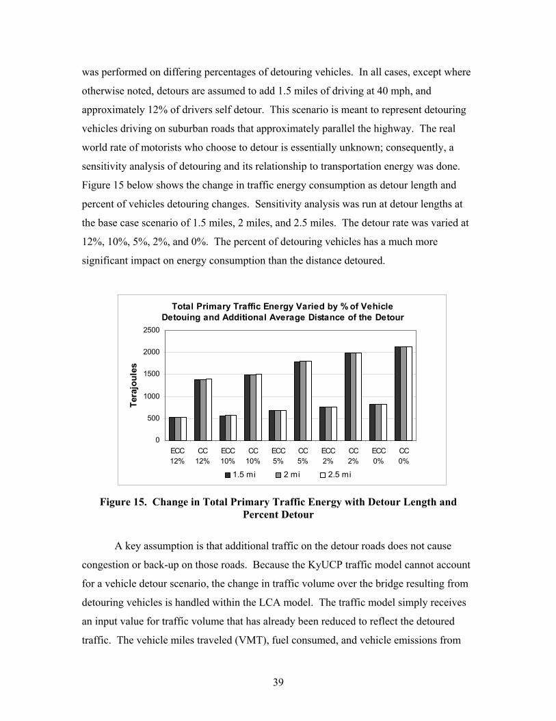
39
was performed on differing percentages of detouring vehicles. In all cases, except where
otherwise noted, detours are assumed to add 1.5 miles of driving at 40 mph, and
approximately 12% of drivers self detour. This scenario is meant to represent detouring
vehicles driving on suburban roads that approximately parallel the highway. The real
world rate of motorists who choose to detour is essentially unknown; consequently, a
sensitivity analysis of detouring and its relationship to transportation energy was done.
Figure 15 below shows the change in traffic energy consumption as detour length and
percent of vehicles detouring changes. Sensitivity analysis was run at detour lengths at
the base case scenario of 1.5 miles, 2 miles, and 2.5 miles. The detour rate was varied at
12%, 10%, 5%, 2%, and 0%. The percent of detouring vehicles has a much more
significant impact on energy consumption than the distance detoured.
Total Primary Traffic Energy Varied by % of Vehicle Detouing and Additional Average Distance of the Detour
0
500
1000
1500
2000
2500
ECC12%
CC12%
ECC10%
CC10%
ECC5%
CC5%
ECC2%
CC2%
ECC0%
CC0%
Tera
joul
es
1.5 mi 2 mi 2.5 mi
Figure 15. Change in Total Primary Traffic Energy with Detour Length and Percent Detour
A key assumption is that additional traffic on the detour roads does not cause
congestion or back-up on those roads. Because the KyUCP traffic model cannot account
for a vehicle detour scenario, the change in traffic volume over the bridge resulting from
detouring vehicles is handled within the LCA model. The traffic model simply receives
an input value for traffic volume that has already been reduced to reflect the detoured
traffic. The vehicle miles traveled (VMT), fuel consumed, and vehicle emissions from
40
detoured vehicles are added to the traffic phase of the LCA model during the vehicle
emissions calculation phase, after the traffic model has been run.
The output from the traffic phase of the LCA model consists of values for fuel
consumption, emissions, and time lost to travelers in congestion. All of these values are
calculated based on their difference from the baseline condition of non-construction
traffic flow. In all cases the following equation is applied to the parameter being
calculated, such as emissions values (mg/mile), time (hour/mile), and fuel use (gal/mile).
These parameters are multiplied by the VMT of each traffic condition, such as VMT in
the traffic queue, or VMT through the work zone. The distance over which VMT is
calculated for the baseline scenario changes with traffic queue length. In the equation
below the parameters are represented by the variable “Y”:
Result (Y) = (VMTQueue*Y+ VMTWork zone*Y + VMTDetour*Y) - VMTBaseline*Y
4.3.4 Macro Logic Sequence for Traffic
The following steps outline the logic sequence for the traffic macros.
1. From LCA_main workbook verify which of the four possible SRC and ECC
material formulations are to be analyzed in the run.
2. From LCA_main collect relevant user-input information such as length of each
construction process, on-road vehicle fleet figures like percent trucks, speed
limits for highway and work zone, detour figures, and the timeline of events.
3. Run the traffic model, housed within the Traffic workbook, for each event
over the 60-year time horizon and copy output for each event into a single
worksheet.
4. Use the output from step 3 to collect emissions data from the MOBILE6 look-
up tables based on speed and year of event. This has to be done for the base
case and the construction case for each event at each year.
5. Calculate fuel consumption and associated CO2 values, calculate their
difference from the baseline values, and add these to the output data.
6. Copy and paste vehicle emissions to LCA_main.
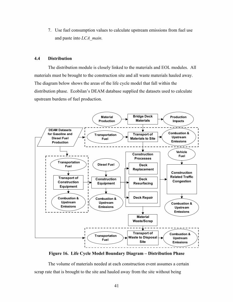
41
7. Use fuel consumption values to calculate upstream emissions from fuel use
and paste into LCA_main.
4.4 Distribution
The distribution module is closely linked to the materials and EOL modules. All
materials must be brought to the construction site and all waste materials hauled away.
The diagram below shows the areas of the life cycle model that fall within the
distribution phase. Ecobilan’s DEAM database supplied the datasets used to calculate
upstream burdens of fuel production.
Construction Processes
Deck Replacement
Deck Resurfacing
Deck Repair
Construction Equipment
Combustion & Upstream Emissions
Diesel Fuel
Construction Related Traffic
Congestion
Material Waste/Scrap
Bridge Deck Materials
Vehicle Fuel
Combustion & Upstream Emissions
Transport ofConstruction
Equipment
Transportation Fuel
Production Impacts
Material Production
Transport ofMaterials to Site
Transportation Fuel
Transport ofWaste to Disposal
Site
Transportation Fuel
DEAM Datasets for Gasoline and
Diesel Fuel Production
Combustion & Upstream Emissions
Combustion & Upstream Emissions
Combustion & Upstream Emissions
Figure 16. Life Cycle Model Boundary Diagram – Distribution Phase The volume of materials needed at each construction event assumes a certain
scrap rate that is brought to the site and hauled away from the site without being
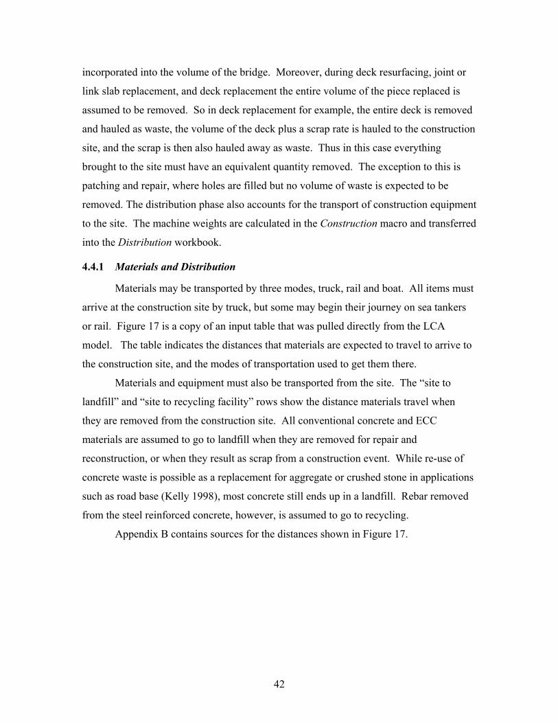
42
incorporated into the volume of the bridge. Moreover, during deck resurfacing, joint or
link slab replacement, and deck replacement the entire volume of the piece replaced is
assumed to be removed. So in deck replacement for example, the entire deck is removed
and hauled as waste, the volume of the deck plus a scrap rate is hauled to the construction
site, and the scrap is then also hauled away as waste. Thus in this case everything
brought to the site must have an equivalent quantity removed. The exception to this is
patching and repair, where holes are filled but no volume of waste is expected to be
removed. The distribution phase also accounts for the transport of construction equipment
to the site. The machine weights are calculated in the Construction macro and transferred
into the Distribution workbook.
4.4.1 Materials and Distribution
Materials may be transported by three modes, truck, rail and boat. All items must
arrive at the construction site by truck, but some may begin their journey on sea tankers
or rail. Figure 17 is a copy of an input table that was pulled directly from the LCA
model. The table indicates the distances that materials are expected to travel to arrive to
the construction site, and the modes of transportation used to get them there.
Materials and equipment must also be transported from the site. The “site to
landfill” and “site to recycling facility” rows show the distance materials travel when
they are removed from the construction site. All conventional concrete and ECC
materials are assumed to go to landfill when they are removed for repair and
reconstruction, or when they result as scrap from a construction event. While re-use of
concrete waste is possible as a replacement for aggregate or crushed stone in applications
such as road base (Kelly 1998), most concrete still ends up in a landfill. Rebar removed
from the steel reinforced concrete, however, is assumed to go to recycling.
Appendix B contains sources for the distances shown in Figure 17.
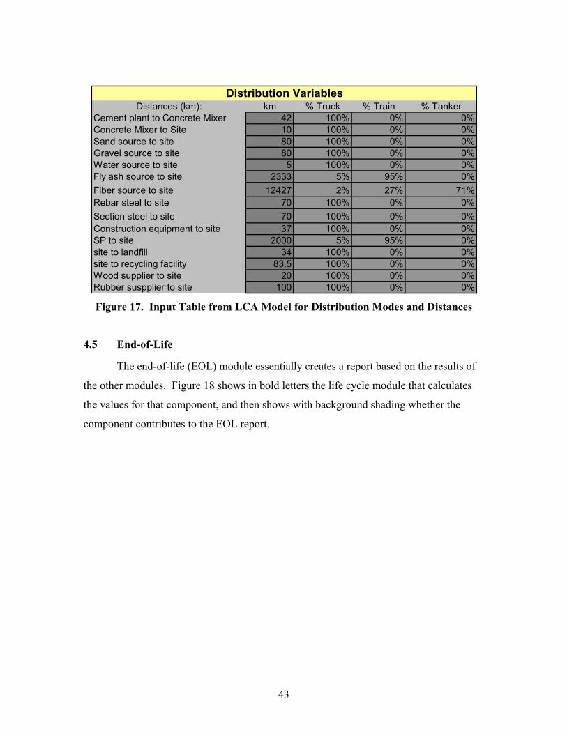
43
Distances (km): km % Truck % Train % TankerCement plant to Concrete Mixer 42 100% 0% 0%Concrete Mixer to Site 10 100% 0% 0%Sand source to site 80 100% 0% 0%Gravel source to site 80 100% 0% 0%Water source to site 5 100% 0% 0%Fly ash source to site 2333 5% 95% 0%Fiber source to site 12427 2% 27% 71%Rebar steel to site 70 100% 0% 0%Section steel to site 70 100% 0% 0%Construction equipment to site 37 100% 0% 0%SP to site 2000 5% 95% 0%site to landfill 34 100% 0% 0%site to recycling facility 83.5 100% 0% 0%Wood supplier to site 20 100% 0% 0%Rubber suspplier to site 100 100% 0% 0%
Distribution Variables
Figure 17. Input Table from LCA Model for Distribution Modes and Distances
4.5 End-of-Life
The end-of-life (EOL) module essentially creates a report based on the results of
the other modules. Figure 18 shows in bold letters the life cycle module that calculates
the values for that component, and then shows with background shading whether the
component contributes to the EOL report.
44
Distribution
Distribution
Materials
Construction
Distribution
Materials
Distribution Construction Processes
Deck Replacement
Deck Resurfacing
Deck Repair
Construction Equipment
Diesel Fuel
Construction Related Traffic
Congestion
Material Waste/Scrap
Vehicle Fuel
Transport ofConstruction
Equipment
Transportation Fuel
Bridge Deck Materials
Production Impacts
Material Production
Transport ofMaterials to Site
Transportation Fuel
Transport ofMaterials to
Disposal Transportation
Fuel
= Contributes to End-of-Life Calculation
Combustion & Upstream Emissions
Combustion & Upstream Emissions
Combustion & Upstream Emissions
Combustion & Upstream Emissions
Combustion & Upstream Emissions
Figure 18. Life Cycle Model Boundary Diagram – End-of-Life Module
EOL accounts for the processes and materials that are part of the disassembly and
disposal of the bridge deck system. The modules that contribute most significantly to the
EOL inventory results are construction and distribution. For example, all construction
processes are calculated in the construction module, but the results are allocated both to
the construction and EOL phases in final reporting based on whether the process removes
a part of the bridge deck or lays new materials in its place. Likewise, distribution is also
split between distribution and EOL in final reporting. When materials are being hauled
away from the construction site, the impacts are allocated to EOL rather than distribution.
45
There is one exception to the EOL reporting method. Construction related traffic
always is reported in the traffic phase and is not ever allocated to the EOL phase –
regardless of whether the construction process underway during the traffic congestion is
allocated to EOL (i.e. bridge deck demolition and removal).
An important assumption in the EOL module is that the ECC and conventional
systems have equal demolition processes. Because of ECC’s durability and resistance to
fracture, demolition could prove more difficult than for conventional concrete. ECC
researchers are still evaluating whether alternative demolition processes will have to be
planned for the material.
4.5.1 Macro Logic Sequence for EOL
The following steps outline the logic sequence for the EOL macros.
1. From LCA_main workbook verify which of the four possible SRC and ECC
material formulations are to be analyzed in the run.
2. Evaluate transportation energy from Distribution that should be allocated to
EOL. This portion includes energy and emissions for waste material transport
away from the construction site to a disposal or recycling site and transport of
construction equipment used in demolition processes.
3. Evaluate construction energy and emissions that should be allocated to EOL
based on the specific construction subprocess. These include removal of
slabs, deck materials, and joints; initial traffic control set-up; scarification; and
hydro. The last two are methods of removing and cleaning the old deck or
surface in preparation for laying a new one.
4. Summarize results from LCI data in LCA_main in EOL. This allocates the
EOL portion of the total in the LCI between EOL and other phases.
46
5 Reference Data and Model Assumptions
5.1 Reference Data
The LCA model’s starting point is the reference datasets for materials. These
datasets provide the basic input values for all the results produced by the model output.
Consistency in terms of what pollutants are produced and what inputs are required for a
given material is important since they are aggregated in life cycle impact calculations.
Moreover, datasets are likely to vary based on region or country. For example, the
production impacts in the United States of producing cement are likely to be different
than those in China or Europe, where production processes and environmental regulations
are different.
The starting point for building a collection of datasets for this model began with
Ecobilan’s DEAM database. (Ecobilan 2001) Ecobilan is a French company that
developed a life cycle analysis database tool that contains data for many materials and
products. In some cases data are available for a single material from multiple world
regions, other times the data are available only from a single region or country. While
U.S. data is preferred it is not always available.
For many other constituents alternative sources were necessary. The Portland
Cement Association (PCA) supplied life cycle data for cement (Nisbet et al. 2002). PCA
is a cement industry organization that has begun addressing and measuring some of the
impacts that the cement industry has on the environment. Data supplied by PCA was
supplemented with DEAM data for a few categories that were not included in PCA data.
Data for the PVA fiber used in ECC was difficult to track down. Full life cycle
data was not available for this material so a hybrid dataset created from data supplied by
the material’s producer and data from the Association of Plastic Manufacturers in Europe
(APME) for polyethylene was used (Bousted 1999). The data fields supplied by the
manufacturer were total primary energy consumption, carbon dioxide emissions, NOx
emissions, SOx emissions, BOD (Biological Oxygen Demand) discharge, COD
(Chemical Oxygen Demand) discharge, and waterborne suspended matter. All other data
categories were substituted with polyethylene data from APME.
47
Superplasticizer data were likewise difficult to trace. Rather than data for this
specific material, data for its precursor formaldehyde were used on an equal-weight basis.
The use of formaldehyde data suggests that, while the LCA dataset should reasonably
characterize superplasticizer, it is a conservative estimate of its total impacts.
Fly ash is considered to be a zero impact material in all categories except waste,
where it has a negative value. Fly ash is a waste product of electricity production and
other coal burning processes. Fly ash is diverted from the waste stream and displaces
cement, thus earning the material a negative waste value. One gap in this data is that fly
ash goes through some processing, such as grinding, before it can be used in cement, thus
there should be some processing and transport energy included in the dataset. Some
potential alternatives to cement and other concrete constituents that are waste products
from industrial processes may be candidates for direct use, and these are being explored
for use in new ECC formulations. Potential materials include industrial waste products
such as green sand from forgery operations. These materials would have no additional
processing energy associated with them. The suitability of these materials as direct
substitutes for concrete constituents is still under evaluation by University of Michigan
researchers at the Advanced Civil Engineering Materials Research Laboratory.
Appendix C provides the datasets used in the LCA model, and Appendix D
provides the sources of the datasets. The datasets discussed above are the most
complicated in so much as they come from compound sources or rely on data substituted
from other materials.
The environmental assessment in this thesis focuses on the following impact
categories; raw material consumptions, energy consumption, criteria air pollutants,
criteria water pollutants, and greenhouse gas emissions. The air pollutants included in
the assessment are methane, carbon monoxide, particulate matter (as PM10),
hydrocarbons, nitrogen oxides, and sulfur oxides. The water emissions included in the
assessment are biological oxygen demand, ammonia, phosphate, oils, suspended matter,
and dissolved matter. The greenhouse gas emissions used to calculate global warming
potential, which is discussed in more detail in section 6.2.1, are CO2, methane, and
nitrous oxide. While many more pollutants were tracked that contribute to environmental
impacts, these emissions were consistently reported throughout all data categories and
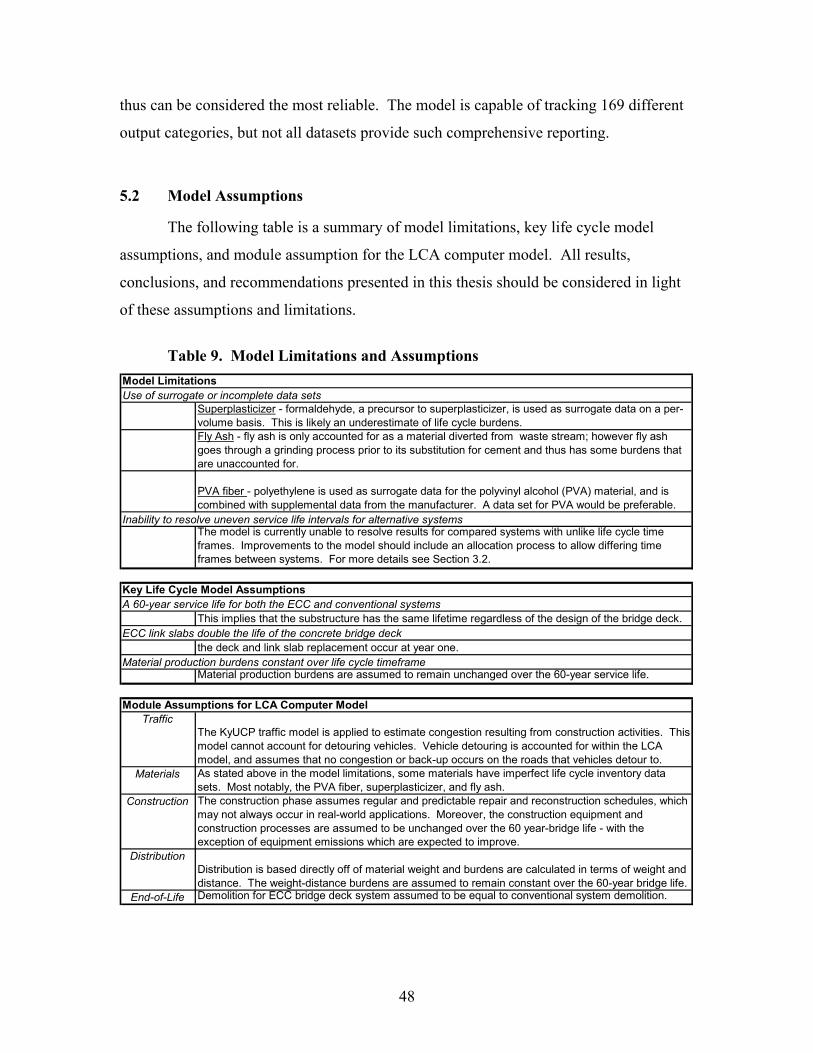
48
thus can be considered the most reliable. The model is capable of tracking 169 different
output categories, but not all datasets provide such comprehensive reporting.
5.2 Model Assumptions
The following table is a summary of model limitations, key life cycle model
assumptions, and module assumption for the LCA computer model. All results,
conclusions, and recommendations presented in this thesis should be considered in light
of these assumptions and limitations.
Table 9. Model Limitations and Assumptions
Model LimitationsUse of surrogate or incomplete data sets
Superplasticizer - formaldehyde, a precursor to superplasticizer, is used as surrogate data on a per-volume basis. This is likely an underestimate of life cycle burdens. Fly Ash - fly ash is only accounted for as a material diverted from waste stream; however fly ash goes through a grinding process prior to its substitution for cement and thus has some burdens that are unaccounted for.
PVA fiber - polyethylene is used as surrogate data for the polyvinyl alcohol (PVA) material, and is combined with supplemental data from the manufacturer. A data set for PVA would be preferable.
Inability to resolve uneven service life intervals for alternative systemsThe model is currently unable to resolve results for compared systems with unlike life cycle time frames. Improvements to the model should include an allocation process to allow differing time frames between systems. For more details see Section 3.2.
Key Life Cycle Model Assumptions
This implies that the substructure has the same lifetime regardless of the design of the bridge deck.
the deck and link slab replacement occur at year one.Material production burdens constant over life cycle timeframe
Material production burdens are assumed to remain unchanged over the 60-year service life.
Module Assumptions for LCA Computer ModelTraffic
The KyUCP traffic model is applied to estimate congestion resulting from construction activities. This model cannot account for detouring vehicles. Vehicle detouring is accounted for within the LCA model, and assumes that no congestion or back-up occurs on the roads that vehicles detour to.
Materials As stated above in the model limitations, some materials have imperfect life cycle inventory data sets. Most notably, the PVA fiber, superplasticizer, and fly ash.
Construction The construction phase assumes regular and predictable repair and reconstruction schedules, which may not always occur in real-world applications. Moreover, the construction equipment and construction processes are assumed to be unchanged over the 60 year-bridge life - with the exception of equipment emissions which are expected to improve.
DistributionDistribution is based directly off of material weight and burdens are calculated in terms of weight and distance. The weight-distance burdens are assumed to remain constant over the 60-year bridge life.
End-of-Life Demolition for ECC bridge deck system assumed to be equal to conventional system demolition.
ECC link slabs double the life of the concrete bridge deck
A 60-year service life for both the ECC and conventional systems
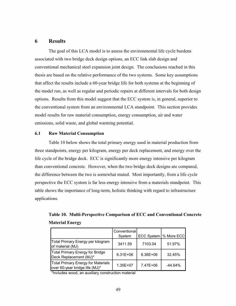
49
6 Results
The goal of this LCA model is to assess the environmental life cycle burdens
associated with two bridge deck design options, an ECC link slab design and
conventional mechanical steel expansion joint design. The conclusions reached in this
thesis are based on the relative performance of the two systems. Some key assumptions
that affect the results include a 60-year bridge life for both systems at the beginning of
the model run, as well as regular and periodic repairs at different intervals for both design
options. Results from this model suggest that the ECC system is, in general, superior to
the conventional system from an environmental LCA standpoint. This section provides
model results for raw material consumption, energy consumption, air and water
emissions, solid waste, and global warming potential.
6.1 Raw Material Consumption
Table 10 below shows the total primary energy used in material production from
three standpoints, energy per kilogram, energy per deck replacement, and energy over the
life cycle of the bridge deck. ECC is significantly more energy intensive per kilogram
than conventional concrete. However, when the two bridge deck designs are compared,
the difference between the two is somewhat muted. Most importantly, from a life cycle
perspective the ECC system is far less energy intensive from a materials standpoint. This
table shows the importance of long-term, holistic thinking with regard to infrastructure
applications.
Table 10. Multi-Perspective Comparison of ECC and Conventional Concrete
Material Energy
Conventional System ECC System % More ECC
Total Primary Energy per kilogram of material (MJ) 3411.59 7103.04 51.97%
Total Primary Energy for Bridge Deck Replacement (MJ)* 6.31E+06 8.36E+06 32.45%
Total Primary Energy for Materials over 60-year bridge life (MJ)* 1.35E+07 7.47E+06 -44.64%
*Includes wood, an auxiliary construction material

50
Table 11 shows the raw material usage for six key materials in the two systems
over the entire 60-year life cycle. Note that while Tables 3 and 4 showed greater cement
content in the ECC formulation over SRC, because ECC is applied strategically and
extends the life of the SRC deck, the ECC system uses considerably less limestone and
other raw materials over the 60-year life cycle of the bridge.
Table 11. Life Cycle Raw Material Resource Use
Raw Material Conventional System (metric tonnes)
ECC System (metric tonnes)
% Less ECC
Coal 124 67 54%Limestone 757 406 54%
Natural Gas 140 84 60%Oil 590 368 62%
Sand 852 443 52%Water 24696 15351 62%
6.2 Energy Consumption
Figure 19 below shows the total primary energy consumed by each life cycle
phase. The traffic phase dominates both the ECC and conventional system results,
followed by the materials phase; these two dominant phases dwarf the construction,
distribution, and EOL phases. In this and all subsequent figures “∆ traffic” is used to
describe the traffic phase as a reminder that the traffic phase only shows the difference
between impacts during construction related traffic congestion and impacts from normal
traffic flow. The conventional system consumes 74874 gigajoules (GJ) in total primary
energy and the ECC system consumes 44764 GJ in total primary energy, a 40% reduction
from the conventional system.
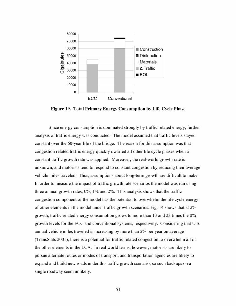
51
0
10000
20000
30000
40000
50000
60000
70000
80000
ECC Conventional
Gig
ajou
les
ConstructionDistributionMaterials∆ Traffic EOL
Figure 19. Total Primary Energy Consumption by Life Cycle Phase
Since energy consumption is dominated strongly by traffic related energy, further
analysis of traffic energy was conducted. The model assumed that traffic levels stayed
constant over the 60-year life of the bridge. The reason for this assumption was that
congestion related traffic energy quickly dwarfed all other life cycle phases when a
constant traffic growth rate was applied. Moreover, the real-world growth rate is
unknown, and motorists tend to respond to constant congestion by reducing their average
vehicle miles traveled. Thus, assumptions about long-term growth are difficult to make.
In order to measure the impact of traffic growth rate scenarios the model was run using
three annual growth rates, 0%, 1% and 2%. This analysis shows that the traffic
congestion component of the model has the potential to overwhelm the life cycle energy
of other elements in the model under traffic growth scenarios. Fig. 14 shows that at 2%
growth, traffic related energy consumption grows to more than 13 and 23 times the 0%
growth levels for the ECC and conventional systems, respectively. Considering that U.S.
annual vehicle miles traveled is increasing by more than 2% per year on average
(TransStats 2001), there is a potential for traffic related congestion to overwhelm all of
the other elements in the LCA. In real world terms, however, motorists are likely to
pursue alternate routes or modes of transport, and transportation agencies are likely to
expand and build new roads under this traffic growth scenario, so such backups on a
single roadway seem unlikely.
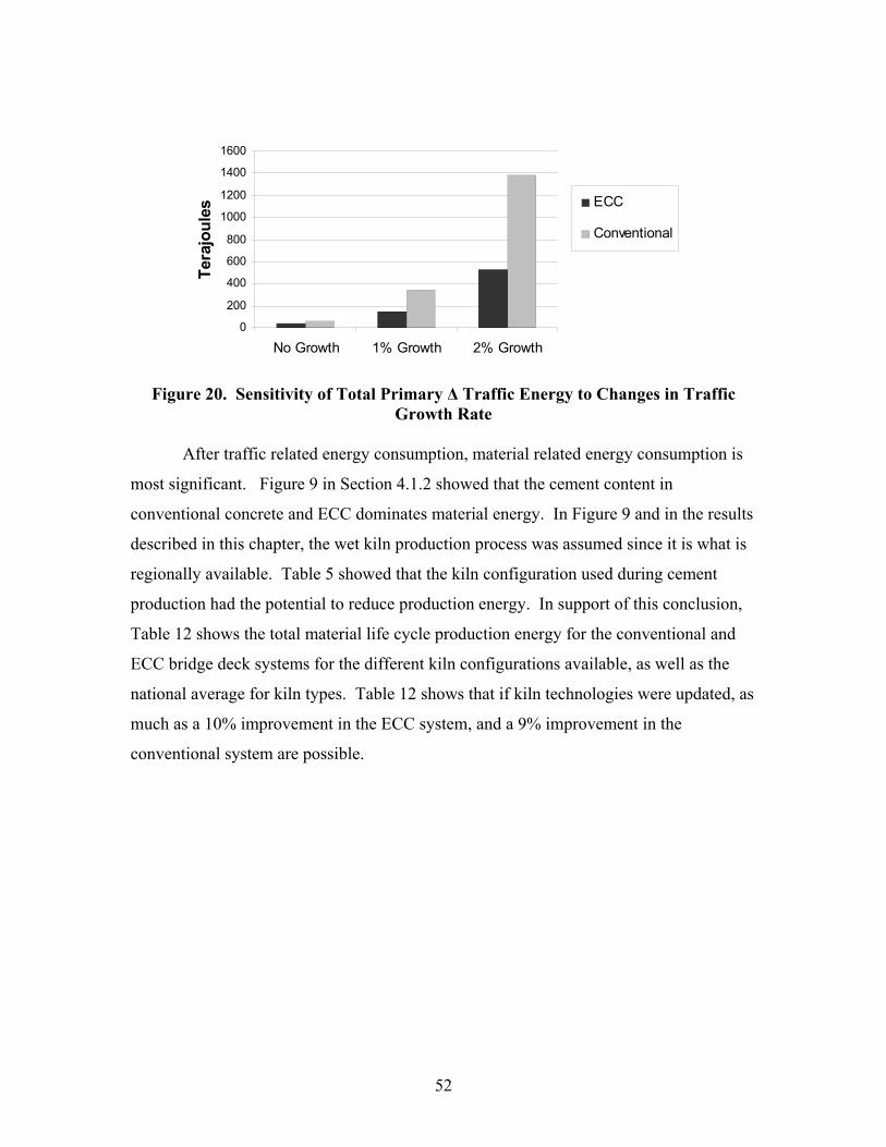
52
0
200
400
600
800
1000
1200
1400
1600
No Growth 1% Growth 2% Growth
Tera
joul
es ECC
Conventional
Figure 20. Sensitivity of Total Primary ∆ Traffic Energy to Changes in Traffic
Growth Rate
After traffic related energy consumption, material related energy consumption is
most significant. Figure 9 in Section 4.1.2 showed that the cement content in
conventional concrete and ECC dominates material energy. In Figure 9 and in the results
described in this chapter, the wet kiln production process was assumed since it is what is
regionally available. Table 5 showed that the kiln configuration used during cement
production had the potential to reduce production energy. In support of this conclusion,
Table 12 shows the total material life cycle production energy for the conventional and
ECC bridge deck systems for the different kiln configurations available, as well as the
national average for kiln types. Table 12 shows that if kiln technologies were updated, as
much as a 10% improvement in the ECC system, and a 9% improvement in the
conventional system are possible.
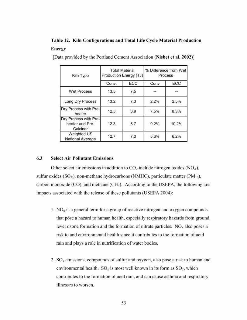
53
Table 12. Kiln Configurations and Total Life Cycle Material Production
Energy
[Data provided by the Portland Cement Association (Nisbet et al. 2002)]
Conv. ECC Conv ECC
Wet Process 13.5 7.5 -- --
Long Dry Process 13.2 7.3 2.2% 2.5%
Dry Process with Pre-heater 12.5 6.9 7.5% 8.3%
Dry Process with Pre-heater and Pre-
Calciner12.3 6.7 9.2% 10.2%
Weighted US National Average 12.7 7.0 5.6% 6.2%
Kiln TypeTotal Material
Production Energy (TJ)% Difference from Wet
Process
6.3 Select Air Pollutant Emissions
Other select air emissions in addition to CO2 include nitrogen oxides (NOX),
sulfur oxides (SOX), non-methane hydrocarbons (NMHC), particulate matter (PM10),
carbon monoxide (CO), and methane (CH4). According to the USEPA, the following are
impacts associated with the release of these pollutants (USEPA 2004):
1. NOx is a general term for a group of reactive nitrogen and oxygen compounds
that pose a hazard to human health, especially respiratory hazards from ground
level ozone formation and the formation of nitrate particles. NOx also poses a
risk to and environmental health since it contributes to the formation of acid
rain and plays a role in nutrification of water bodies.
2. SOx emissions, compounds of sulfur and oxygen, also pose a risk to human and
environmental health. SOx is most well known in its form as SO2, which
contributes to the formation of acid rain, and can cause asthma and respiratory
illnesses to worsen.
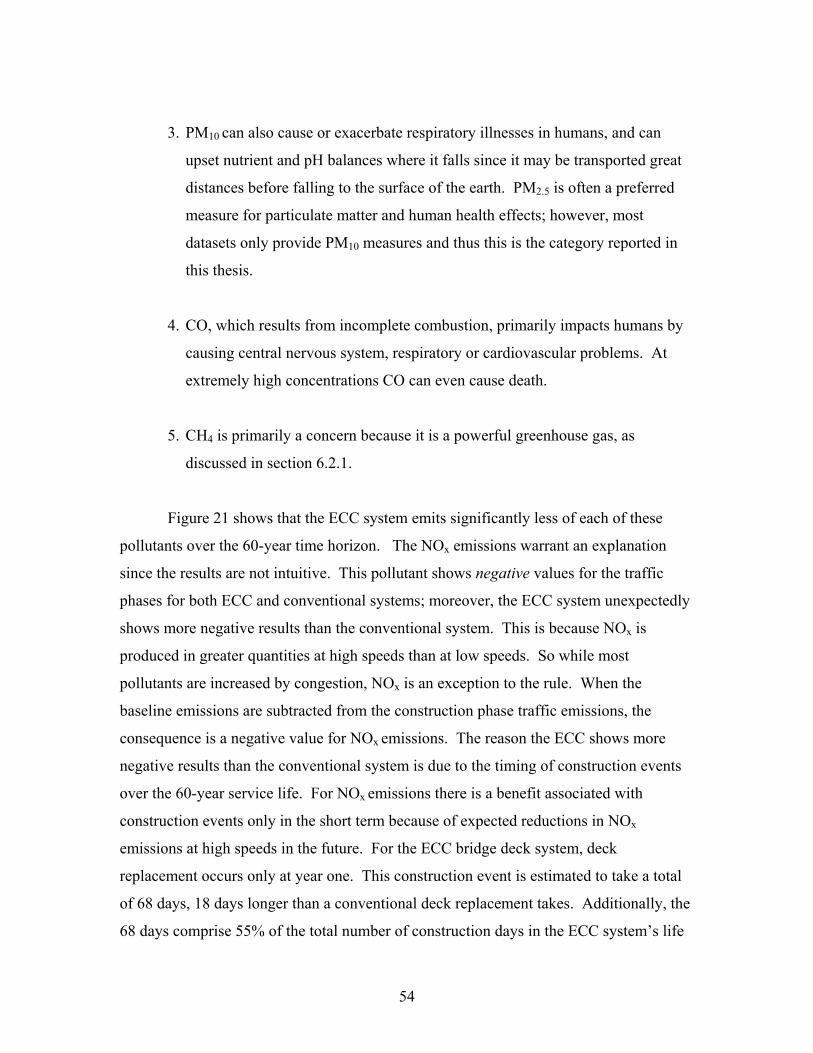
54
3. PM10 can also cause or exacerbate respiratory illnesses in humans, and can
upset nutrient and pH balances where it falls since it may be transported great
distances before falling to the surface of the earth. PM2.5 is often a preferred
measure for particulate matter and human health effects; however, most
datasets only provide PM10 measures and thus this is the category reported in
this thesis.
4. CO, which results from incomplete combustion, primarily impacts humans by
causing central nervous system, respiratory or cardiovascular problems. At
extremely high concentrations CO can even cause death.
5. CH4 is primarily a concern because it is a powerful greenhouse gas, as
discussed in section 6.2.1.
Figure 21 shows that the ECC system emits significantly less of each of these
pollutants over the 60-year time horizon. The NOx emissions warrant an explanation
since the results are not intuitive. This pollutant shows negative values for the traffic
phases for both ECC and conventional systems; moreover, the ECC system unexpectedly
shows more negative results than the conventional system. This is because NOx is
produced in greater quantities at high speeds than at low speeds. So while most
pollutants are increased by congestion, NOx is an exception to the rule. When the
baseline emissions are subtracted from the construction phase traffic emissions, the
consequence is a negative value for NOx emissions. The reason the ECC shows more
negative results than the conventional system is due to the timing of construction events
over the 60-year service life. For NOx emissions there is a benefit associated with
construction events only in the short term because of expected reductions in NOx
emissions at high speeds in the future. For the ECC bridge deck system, deck
replacement occurs only at year one. This construction event is estimated to take a total
of 68 days, 18 days longer than a conventional deck replacement takes. Additionally, the
68 days comprise 55% of the total number of construction days in the ECC system’s life
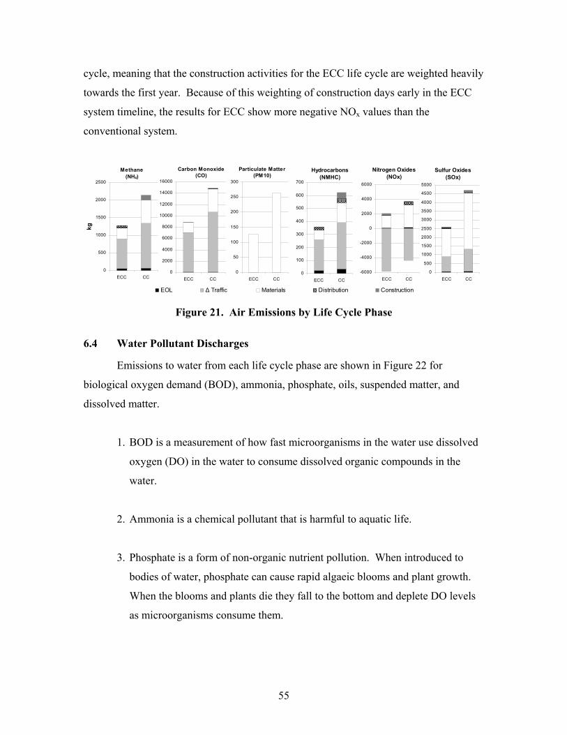
55
cycle, meaning that the construction activities for the ECC life cycle are weighted heavily
towards the first year. Because of this weighting of construction days early in the ECC
system timeline, the results for ECC show more negative NOx values than the
conventional system.
Methane
(NH4)
0
500
1000
1500
2000
2500
ECC CC
kg
EOL ∆ Traffic Materials Distribution Construction
Carbon Monoxide(CO)
0
2000
4000
6000
8000
10000
12000
14000
16000
ECC CC
Particulate Matter (PM10)
0
50
100
150
200
250
300
ECC CC
Hydrocarbons (NMHC)
0
100
200
300
400
500
600
700
ECC CC
Nitrogen Oxides (NOx)
-6000
-4000
-2000
0
2000
4000
6000
ECC CC
Sulfur Oxides (SOx)
0
500
1000
1500
2000
2500
3000
3500
4000
4500
5000
ECC CC
Figure 21. Air Emissions by Life Cycle Phase
6.4 Water Pollutant Discharges
Emissions to water from each life cycle phase are shown in Figure 22 for
biological oxygen demand (BOD), ammonia, phosphate, oils, suspended matter, and
dissolved matter.
1. BOD is a measurement of how fast microorganisms in the water use dissolved
oxygen (DO) in the water to consume dissolved organic compounds in the
water.
2. Ammonia is a chemical pollutant that is harmful to aquatic life.
3. Phosphate is a form of non-organic nutrient pollution. When introduced to
bodies of water, phosphate can cause rapid algaeic blooms and plant growth.
When the blooms and plants die they fall to the bottom and deplete DO levels
as microorganisms consume them.
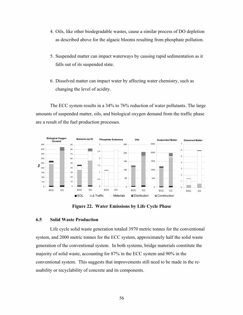
56
4. Oils, like other biodegradable wastes, cause a similar process of DO depletion
as described above for the algaeic blooms resulting from phosphate pollution.
5. Suspended matter can impact waterways by causing rapid sedimentation as it
falls out of its suspended state.
6. Dissolved matter can impact water by affecting water chemistry, such as
changing the level of acidity.
The ECC system results in a 34% to 76% reduction of water pollutants. The large
amounts of suspended matter, oils, and biological oxygen demand from the traffic phase
are a result of the fuel production processes.
Dissolved Matter
0
1
2
3
4
5
6
7
ECC CC
EOL ∆ Traffic Materials Distribution Construction
Biological Oxygen Demand
0
50
100
150
200
250
300
350
400
450
ECC CC
kg
Ammonia (as N)
0
10
20
30
40
50
60
70
80
90
ECC CC
Phosphate Emissions
0
0.5
1
1.5
2
2.5
3
ECC CC
Oils
0
50
100
150
200
250
ECC CC
Suspended Matter
0
500
1000
1500
2000
2500
ECC CC
Figure 22. Water Emissions by Life Cycle Phase
6.5 Solid Waste Production
Life cycle solid waste generation totaled 3970 metric tonnes for the conventional
system, and 2000 metric tonnes for the ECC system, approximately half the solid waste
generation of the conventional system. In both systems, bridge materials constitute the
majority of solid waste, accounting for 87% in the ECC system and 90% in the
conventional system. This suggests that improvements still need to be made in the re-
usability or recyclability of concrete and its components.
57
6.6 Greenhouse Gas Emissions
The results of greenhouse gas (GHG) emissions are similar to those for energy
consumption. Traffic related carbon dioxide (CO2) dominates total GHG emissions for
both the ECC and conventional bridge systems. Material production is the only other
significant contributor. Figure 23 shows the total greenhouse gas emissions in metric
tonnes of CO2 equivalent for each system. This is calculated by multiplying the mass of
each GHG emission by its global warming potential (GWP). The GWP’s are based on
the radiative forcing (heat absorbing ability) of each GHG as well as the decay rate of
each gas relative to carbon dioxide over a 100-year time horizon. The GHG emissions
included in this analysis are CO2 (GWP = 1), methane (GWP = 23), and nitrous oxide
(GWP = 296) (Houghton 2001). Despite the contribution to global warming of the two
other gases, CO2 overwhelmingly dominates GWP results. In the ECC system CO2
represents 98% of total life cycle GWP, and in the conventional system CO2 represents
99% of total life cycle GWP. The ECC system shows a reduction of 33% in GWP over
the conventional system. Typically, CO2 emissions mirror energy consumption; however,
the production of cement involves the release of additional CO2 during pyroprocessing
(conversion of calcium carbonate to calcium oxide), which results in twice the CO2 that
would be produced from energy consumption alone (CEMBUREAU 1998). This
additional contribution of CO2 from cement production is evident in the comparison of
Figures 19 and 23 wherein material production represents a greater portion of the total
CO2 emissions than it does total energy consumption.
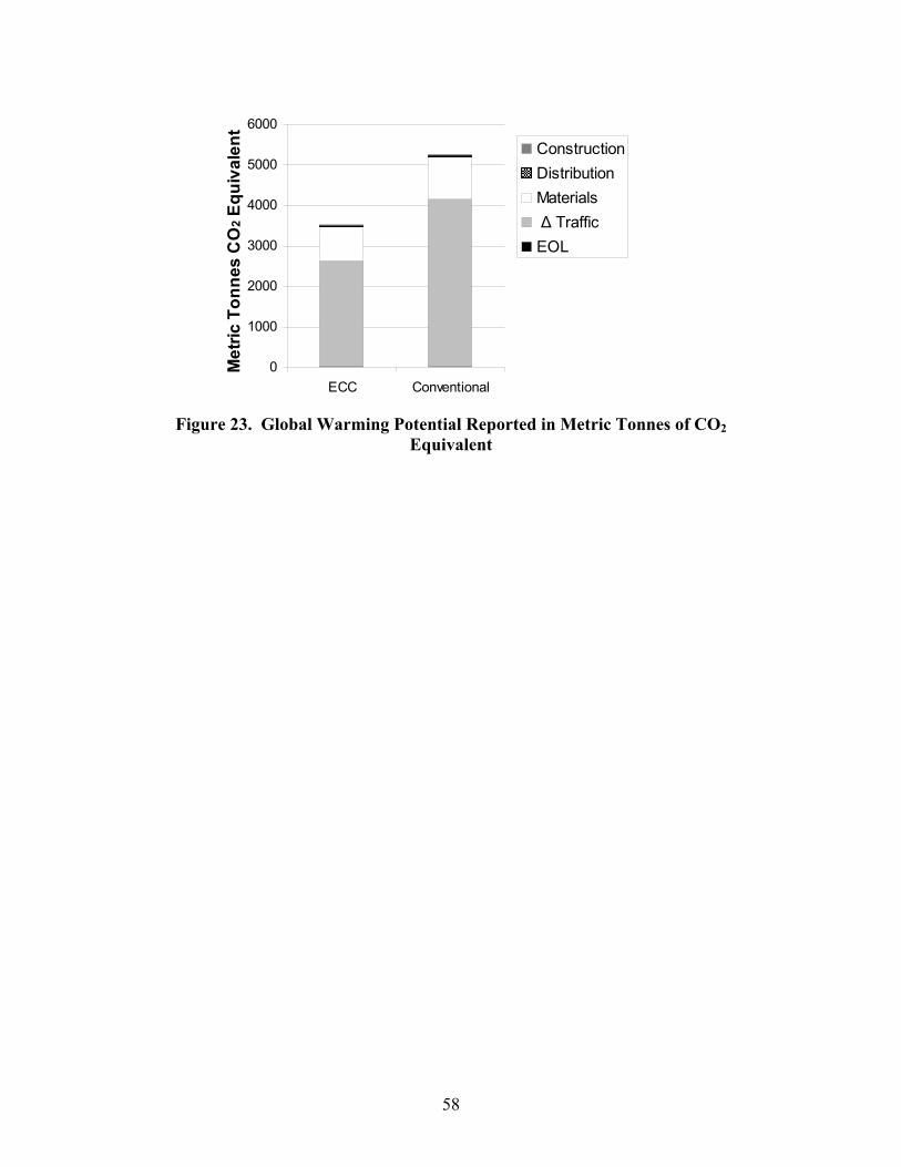
58
0
1000
2000
3000
4000
5000
6000
ECC Conventional
Met
ric T
onne
s C
O 2 E
quiv
alen
t
ConstructionDistributionMaterials ∆ Traffic EOL
Figure 23. Global Warming Potential Reported in Metric Tonnes of CO2
Equivalent
59
7 Conclusions and Recommendations for Future Research
7.1 Conclusions
This thesis defines a framework and computer modeling approach for the life
cycle assessment of alternative concrete bridge deck designs. The following conclusions
address key features of the model, and results and conclusions from the application of the
model to two bridge deck design alternatives; an ECC link slab design and a conventional
mechanical steel expansion joint design. Results should be considered in light of the
assumptions and limitations of the model as outlined in Table 9.
1. An expanded scope over previous LCA studies.
This model broadens the scope of bridge LCA studies by accounting for the
dynamic nature of the interlinked bridge and traffic systems. The traffic system proved
to be the most significant contributor to many categories in the LCA results; thus, this
new scope is an important development in LCA applications to bridges and similar
infrastructure systems.
2. LCA model flexibility.
With over 100 flexible parameters programmed in the LCA computer model,
users can explore the impacts of changes in material formulation and properties as well as
test the sensitivity of the model with regard to key assumptions. Testing the impacts of
material choice on long-term applications is a key feature in improving infrastructure
sustainability. Moreover, sensitivity analysis allows for improved assessment of the
reliability of model results.
3. The ECC link slab system resulted in significantly lower environmental
impacts.
Over a 60-year service life, the ECC system resulted in a savings of more than
50% in materials and energy compared to the conventional system. This results primarily
from the reduced number of repair and reconstruction events modeled for the ECC
system.
60
4. Construction related traffic proved to be a key determinant of environmental
impact.
A key finding from life cycle modeling was the importance of construction related
traffic on the environmental performance of both deck systems. In the baseline scenario
of 0% traffic growth over the 60-year service life of the bridge, construction related
traffic energy comprised 80% of total primary life cycle energy for the conventional
system and 85% of total primary life cycle energy in the ECC system. Traffic related air
emissions also dominate results for carbon monoxide, methane, hydrocarbons, and
greenhouse gas emissions in the form of carbon dioxide.
Figure 20 showed that when traffic growth was varied between 0 and 2%, changes
in the amount of total primary energy consumed by the phase increased by 130% and
230% for the ECC and conventional systems, respectively. Because of the significant
impact that traffic has on the LCA results, assessing long term traffic growth patterns and
accurately predicting maintenance and repair schedules for a system is critical to
evaluating the performance of alternative materials.
In order to address some of the uncertainty in traffic modeling, a sensitivity
analysis was performed in Section 4.4.3. The analysis showed that the volume of vehicle
traffic that detoured had more impact on energy consumption than the length of the
detour. This suggests that improved traffic management and planning during
construction events could reduce the impact of construction related traffic, as long as
significant congestion does not occur on detour routes.
5. Strategic application of ECC material results in improved environmental
performance.
This model showed that, while ECC is more energy intensive on a per mass basis,
its strategic application in a bridge deck as link slabs reduces overall material energy
consumption, raw material consumption, air pollution, water pollution, greenhouse gas
emissions, and total primary energy consumption over the life cycle of the bridge deck.
61
6. Improvements in the sustainability of infrastructure will require improved
material selection criteria.
The significant improvements of the ECC system over the conventional system
forecasted by this model show the need for updated policy and removal of institutional
barriers to allow for novel materials and designs to be incorporated in road construction.
Improving durability of road systems is especially important because of the diverse
nature of impacts, and the long-lived nature and consequences of infrastructure systems.
7. This model can facilitate additional research of ECC or other novel material
applications in infrastructure systems.
Lessons-learned from this modeling, like understanding the difficulty of
determining how to approach life cycle timeframes of different systems, will make future
modeling more streamlined.
7.2 Future Research
An exploration of the deficiencies of this model framework, as well as integration of
the other elements of sustainability, namely economic and social impacts, would yield a
more holistic measure of the benefits of one bridge system over another. The following
are suggestions for future research themes:
1. Fully integrate the LCA model with a life cycle cost (LCC) model.
A fully integrated LCC model would serve as a tool for evaluating the bridge deck
infrastructure from a holistic sustainability perspective – integrating environmental,
social and economic indicators. Such a model could enhance infrastructure sustainability
and investment decisions (Norris 2001).
LCA and LCC models have previously been integrated for several other product
systems including automotive parts (Keoleian and Kar 2003) and photovoltaics (Keoleian
and Lewis 2003). The LCA model is essential to measure the magnitude of the pollution
externalities that can be monetized using unit damage costs from environmental
economics. The infrastructure system investigated in this study, however, represents a
62
greater modeling challenge given its complexity in terms of the continual material and
capital investments over a long service life.
2. Model additional concrete infrastructure systems such as roadways and
concrete pipe.
While the LCA computer model is tailored to this specific bridge deck
application, its dynamic nature and the larger integrated framework of macro-scale
modeling and microscale tailoring can be applied to other infrastructure systems such as
roadways and concrete pipe.
3. Consider changes over time in material production energy intensities and
emissions factors in future modeling.
The impacts of material production and distribution may change over time.
Future model refinements should include adding modeling capability to vary material
production burdens over time.
4. Expand the scope of the LCA model to include other advanced materials.
ECC is only one of many other advanced materials that can be applied to improve
the life cycle performance of bridge decks and other concrete infrastructure systems.
Additional research and modeling can be pursued for other advanced materials, as well as
additional ECC formulations with enhanced performance from mechanical and
environmental standpoints.
5. The effect of ECC link slabs on bridge deck life warrants further
investigation.
This analysis was predicated on the assumption that the ECC link slab would
double the life expectancy of the bridge deck relative to the conventional steel joint.
Different assumptions about the effect of ECC link slabs on bridge deck life are expected
to change the results of this model significantly. This highlights the need for continued
testing of ECC and other new materials to accurately model their long-term impacts.

63
6. Continue and expand current testing of ECC performance and durability.
While researchers have completed countless laboratory tests and initiated one on-
site application of an ECC link slab, many questions still remain with regard to the ECC
system’s effectiveness in extending the life of the concrete bridge deck. Continued
laboratory testing as well as real-world site testing is necessary to confirm or challenge
the assumptions about durability and repair of the ECC link slab system.
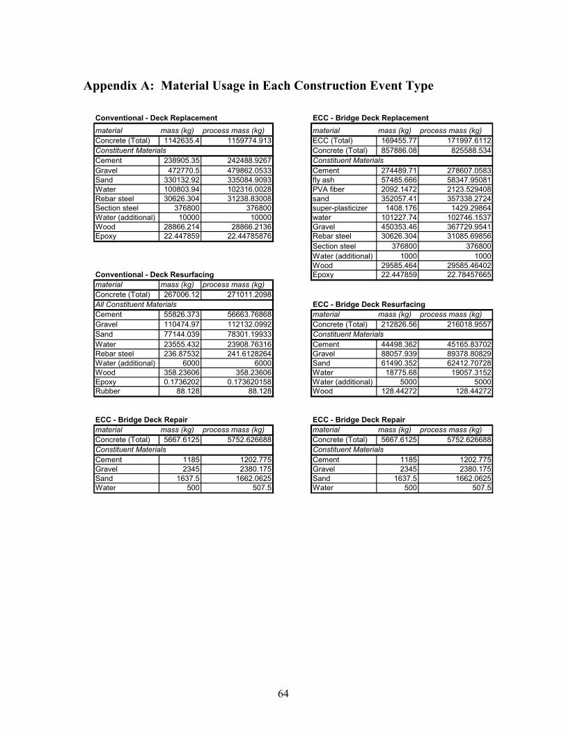
64
Appendix A: Material Usage in Each Construction Event Type
Conventional - Deck Replacement ECC - Bridge Deck Replacementmaterial mass (kg) process mass (kg) material mass (kg) process mass (kg)Concrete (Total) 1142635.4 1159774.913 ECC (Total) 169455.77 171997.6112Constituent Materials Concrete (Total) 857886.08 825588.534Cement 238905.35 242488.9267 Constituent MaterialsGravel 472770.5 479862.0533 Cement 274489.71 278607.0583Sand 330132.92 335084.9093 fly ash 57485.666 58347.95081Water 100803.94 102316.0028 PVA fiber 2092.1472 2123.529408Rebar steel 30626.304 31238.83008 sand 352057.41 357338.2724Section steel 376800 376800 super-plasticizer 1408.176 1429.29864Water (additional) 10000 10000 water 101227.74 102746.1537Wood 28866.214 28866.2136 Gravel 450353.46 367729.9541Epoxy 22.447859 22.44785876 Rebar steel 30626.304 31085.69856
Section steel 376800 376800Water (additional) 1000 1000Wood 29585.464 29585.46402
Conventional - Deck Resurfacing Epoxy 22.447859 22.78457665material mass (kg) process mass (kg)Concrete (Total) 267006.12 271011.2098All Constituent Materials ECC - Bridge Deck ResurfacingCement 55826.373 56663.76868 material mass (kg) process mass (kg)Gravel 110474.97 112132.0992 Concrete (Total) 212826.56 216018.9557Sand 77144.039 78301.19933 Constituent MaterialsWater 23555.432 23908.76316 Cement 44498.362 45165.83702Rebar steel 236.87532 241.6128264 Gravel 88057.939 89378.80829Water (additional) 6000 6000 Sand 61490.352 62412.70728Wood 358.23606 358.23606 Water 18775.68 19057.3152Epoxy 0.1736202 0.173620158 Water (additional) 5000 5000Rubber 88.128 88.128 Wood 128.44272 128.44272
ECC - Bridge Deck Repair ECC - Bridge Deck Repairmaterial mass (kg) process mass (kg) material mass (kg) process mass (kg)Concrete (Total) 5667.6125 5752.626688 Concrete (Total) 5667.6125 5752.626688Constituent Materials Constituent MaterialsCement 1185 1202.775 Cement 1185 1202.775Gravel 2345 2380.175 Gravel 2345 2380.175Sand 1637.5 1662.0625 Sand 1637.5 1662.0625Water 500 507.5 Water 500 507.5
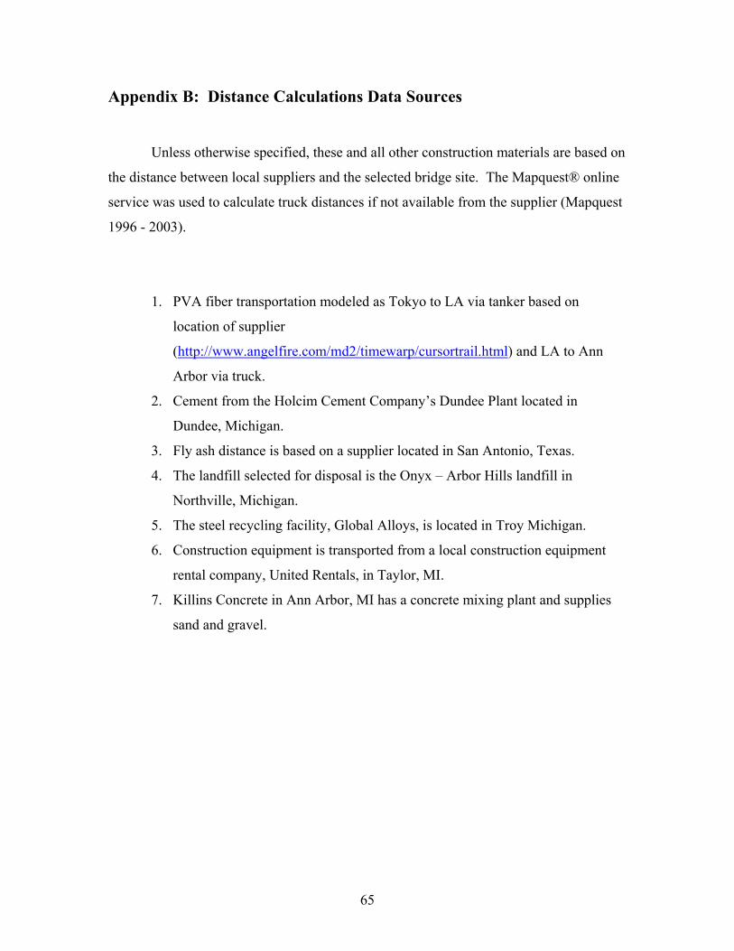
65
Appendix B: Distance Calculations Data Sources
Unless otherwise specified, these and all other construction materials are based on
the distance between local suppliers and the selected bridge site. The Mapquest® online
service was used to calculate truck distances if not available from the supplier (Mapquest
1996 - 2003).
1. PVA fiber transportation modeled as Tokyo to LA via tanker based on
location of supplier
(http://www.angelfire.com/md2/timewarp/cursortrail.html) and LA to Ann
Arbor via truck.
2. Cement from the Holcim Cement Company’s Dundee Plant located in
Dundee, Michigan.
3. Fly ash distance is based on a supplier located in San Antonio, Texas.
4. The landfill selected for disposal is the Onyx – Arbor Hills landfill in
Northville, Michigan.
5. The steel recycling facility, Global Alloys, is located in Troy Michigan.
6. Construction equipment is transported from a local construction equipment
rental company, United Rentals, in Taylor, MI.
7. Killins Concrete in Ann Arbor, MI has a concrete mixing plant and supplies
sand and gravel.
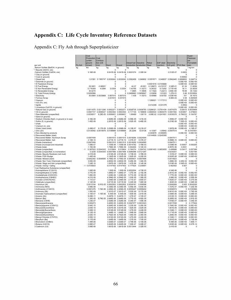
66
Appendix C: Life Cycle Inventory Reference Datasets Appendix C: Fly Ash through Superplasticizer
per unit Fly Ash
Coal Production (under-ground mined)
Coal Combus-tion (US mix) Sand Gravel
Diesel fuel production
Gasoline production
Rebar Steel
EAF steel (section)
Electricity (US grid) PVA fiber
Super-Plastcizer (as Formaldehyde)
1 Barium Sulfate (BaSO4, in ground) kg MJ kg kg kg kg kg kg MJ kg kg 1 kg-km1 Bauxite (Al2O3, ore) 0 0 0 01 Calcium Sulfate (CaSO4, ore) 5.16E-08 8.041E-08 8.041E-08 0.0001074 2.30E-04 2.212E-07 0.0003 01 Clay (in ground) 0 0 0 01 Coal (in ground) 0 0 0.00002 01 Diesel fuel 1.01581 0.1365747 0.0030043 0.0030043 0.0362456 0.048802 0.0291671 0.048937 0.0942445 0.0898693 0.2447141 Dolomite (in ground) 0 0 0.00E+00 0.00E+001 E Feedstock Energy 0 0 0.0001819 0.0105666 0.00E+00 0.00E+001 E Fuel Energy 29.3401 -3.98501 0 0 44.37 45.901 0.126673 -0.219137 2.54E-01 61.34 11.60361 E Non Renewable Energy 0.716309 4.0384 0.0354 0.0354 7.43795 11.9273 8.28332 9.73292 3.77E+00 18.11 23.56391 E Renewable Energy 30.0215 0 0 7.3885 11.8606 6.11824 7.22213 3.90E+00 78.99 35.13421 E Total Primary Energy 0.0200566 0 0 0.0489663 0.0658947 2.03658 1.91223 1.27E-01 0.46 0.03336541 Electricity 30.0564 0.0533869 0.067015 0.067015 7.438 11.9273 8.40989 9.50192 4.03E+00 101 35.16751 Ferrous Scrap 0.031615 0.031615 9.80E-03 2.58 0.2649281 Gypsum 0 0 1.1289021 1.1177213 0.00E+00 0.00E+001 Iron (Fe, ore) 0 0 0.00E+00 0.00E+001 lignite 0 0 -0.014308 -0.031379 0.0002 01 Limestone (CaCO3, in ground) 0 0 0.00E+00 0.00E+001 Natural Gas (in ground) 0.0011675 0.0211206 0.0002371 0.0002371 0.0028735 0.0038783 0.0286321 0.0781434 0.0074379 0.00015 0.00338081 Oil (in ground) 0.0007727 0.0006527 0.0002302 0.0002302 0.117135 0.188909 0.0690544 0.0605479 0.0047492 0.833857 0.4788431 Raw Materials (unspecified) 0.0030917 8.29E-05 0.0008401 0.0008401 1.06489 1.08119 4.69E-02 0.0241601 0.0035578 0.796222 0.1047671 Sand (in ground) 0 0 0 01 Sodium Chloride (NaCl, in ground or in sea) 3.16E-08 4.928E-08 4.928E-08 6.58E-05 1.41E-04 1.355E-07 0.00E+00 01 Sulfur (S, in ground) 1.45E-08 2.261E-08 2.261E-08 3.02E-05 6.48E-05 6.219E-08 7.00E-03 0.00E+001 shale 0 0 0.00E+00 0.00E+001 Uranium (U, ore) 0 0 0.00E+00 0.00E+001 Water Used (total) 2.49E-07 9.17E-09 5.058E-08 5.058E-08 6.10E-07 8.21E-07 1.587E-06 0.00E+00 4.16E-071 Zinc (Zn) 0.0130042 0.0019478 0.0189666 0.0189666 25.2244 53.9136 4.13307 1.05942 0.0547514 18 0.01616012 Non-Allocted by products 0 0 -0.003678 -0.006955 0.00E+00 0.00E+002 Recovered Matter (total) 0 0 0.0144609 0.0245395 0 02 Recovered Matter: Aluminum Scrap 0.0007458 0.0001515 0.0001515 0.0018264 0.0024594 0.0047511 0 02 Recovered Matter: Ash 2.10E-10 3.271E-10 3.271E-10 4.37E-07 9.37E-07 8.998E-10 0.00E+00 0.00E+002 Waste (hazardous) 0.0007458 0.0001515 0.0001515 0.0018259 0.0024585 0.0047511 0 02 Waste (municipal and industrial) 7.08E-07 1.105E-06 1.105E-06 0.0014762 3.16E-03 3.039E-06 0.00007 0.0002052 Waste (total) 1.15E-06 1.799E-06 1.799E-06 0.002404 5.14E-03 4.957E-06 0.0031 02 Waste (unspecified) -1 0.397933 0.0344343 0.015804 0.015804 0.194374 0.264742 0.0061403 0.0653055 0.495688 0.03417 0.0573892 Waste (unspecified, to incineration) 0.3238 0.0344343 0.0007466 0.0007466 0.0090098 0.0121297 0.0234201 0 0.0571842 Waste: Bauxite Residues (red mud) 2.41E-08 2.914E-08 2.914E-08 3.73E-05 3.78E-05 1.161E-07 0.00E+00 0.00E+002 Waste: FGD Sludge 1.40E-08 2.182E-08 2.182E-08 2.92E-05 6.25E-05 6.002E-08 0.00E+00 0.00E+002 Waste: Mineral (inert) 0.0002342 0.0048585 4.756E-05 4.756E-05 0.0005631 0.0007696 0.0014923 0 02 Waste: Non Toxic Chemicals (unspecified) 3.00E-09 4.683E-09 4.683E-09 6.26E-06 1.34E-05 1.288E-08 2.20E-02 0.00E+002 Waste: Slags and Ash (unspecified) 7.04E-10 1.097E-09 1.097E-09 1.47E-06 3.14E-06 3.019E-09 2.00E-03 0.00E+002 Waste: mining + tailing -1 0.0725833 0.0147402 0.0147402 0.177624 0.239091 0.462402 0.007 03 (ar) Radioactive Substance (unspecified) 0 0 0 03 Acenaphthene (C12H10) 1.06E-06 1.65E-06 1.65E-06 0.0022054 4.73E-03 4.54E-06 0 03 Acenaphthylene (C12H8) 3.77E-09 1.089E-07 1.089E-07 1.37E-08 2.15E-08 2.401E-08 0.00E+00 0.00E+003 Acetaldehyde (CH3CHO) 1.85E-09 1.228E-06 1.228E-06 5.71E-09 8.16E-09 1.177E-08 0.00E+00 0.00E+003 Acetophenone (C8H8O) 4.21E-06 4.394E-05 4.394E-05 1.03E-05 1.39E-05 2.68E-05 0.00E+00 2.55E-063 Acrolein (CH2CHCHO) 1.11E-07 2.248E-08 2.248E-08 2.71E-07 3.65E-07 7.052E-07 0.00E+00 5.27E-083 Aldehyde (unspecified) 2.14E-06 5.671E-06 5.671E-06 5.24E-06 7.06E-06 1.363E-05 0.00E+00 2.08E-083 Aluminum (Al) 0.0013194 6.91E-05 0.0002502 0.0002502 0.0038181 0.006596 0.0048269 0.005 0.00420263 Ammonia (NH3) 3.58E-08 4.336E-08 4.336E-08 5.55E-05 5.63E-05 1.727E-07 0.00E+00 7.23E-083 Anthracene (C14H10) 0.0001476 1.74E-06 2.456E-05 2.456E-05 0.0055247 0.0098402 0.0006574 0 0.01835663 Antimony (Sb) 1.55E-09 2.301E-07 2.301E-07 5.53E-09 8.17E-09 9.901E-09 0.00E+00 2.79E-083 Aromatic Hydrocarbons (unspecified) 3.15E-07 1.10E-06 6.45E-08 6.45E-08 1.60E-06 2.81E-06 2.006E-06 0.00E+00 5.08E-053 Arsenic (As) 6.09E-11 9.497E-11 9.497E-11 1.27E-07 2.72E-07 2.612E-10 0.00E+00 0.00E+003 Barium (Ba) 1.30E-05 9.79E-05 2.648E-06 2.648E-06 3.77E-05 4.92E-05 8.285E-05 0.00E+00 2.91E-053 Benzene (C6H6) 1.23E-07 2.528E-08 2.528E-08 8.34E-07 1.49E-06 7.816E-07 0.00E+00 3.34E-053 Benzo(a)anthracene 0.000273 9.465E-05 9.465E-05 0.0367077 0.0633323 0.0017038 0 0.1776243 Benzo(a)pyrene (C20H12) 5.94E-10 6.094E-08 6.094E-08 3.23E-09 5.29E-09 3.784E-09 0.00E+00 0.00E+003 Benzo(b)fluoranthene 2.83E-10 5.637E-08 5.637E-08 1.82E-09 2.62E-09 1.801E-09 0.00E+00 0.00E+003 Benzo(bjk)fluoranthene 3.50E-12 9.912E-08 9.912E-08 1.27E-09 2.24E-09 2.104E-11 0.00E+00 0.00E+003 Benzo(ghi)perylene 8.12E-10 1.648E-10 1.648E-10 1.99E-09 2.68E-09 5.171E-09 0.00E+00 0.00E+003 Benzo(k)fluoranthene 2.02E-10 6.762E-08 6.762E-08 1.44E-09 2.36E-09 1.284E-09 0.00E+00 0.00E+003 Benzyl Chloride (C7H7Cl) 3.50E-12 9.912E-08 9.912E-08 1.27E-09 2.24E-09 2.104E-11 0.00E+00 0.00E+003 Beryllium (Be) 5.17E-06 1.049E-06 1.049E-06 1.27E-05 1.70E-05 3.291E-05 0.00E+00 2.73E-083 Bromoform (CHBr3) 1.49E-06 3.026E-07 3.026E-07 3.79E-06 5.15E-06 9.49E-06 0.00E+00 1.85E-113 Butane (C4H10) 2.88E-07 5.845E-08 5.845E-08 7.05E-07 9.49E-07 1.833E-06 0.00E+00 8.57E-143 Cadmium (Cd) 3.99E-06 1.681E-06 1.681E-06 0.0013444 2.32E-03 2.41E-05 0 0
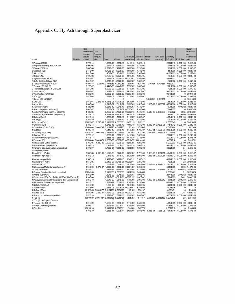
67
Appendix C. Fly Ash through Superplasticizer
3 Propane (C3H8) 6.77E-14 1.055E-13 1.055E-13 1.41E-10 3.02E-10 2.902E-13 0.00E+00 5.91E-083 Propionaldehyde (CH3CH2CHO) 1.80E-06 3.654E-07 3.654E-07 4.50E-06 6.10E-06 1.146E-05 0.00E+00 0.00E+003 Pyrene (C16H10) 2.80E-06 2.727E-05 2.727E-05 6.87E-06 9.25E-06 1.786E-05 0.00E+00 2.30E-073 Selenium (Se) 2.44E-09 8.723E-07 8.723E-07 9.50E-09 1.43E-08 1.557E-08 0.00E+00 0.00E+003 Silicon (Si) 9.62E-06 1.954E-06 1.954E-06 2.53E-05 3.36E-05 6.127E-05 0.00E+00 6.25E-113 Sodium (Na) 3.10E-08 3.757E-08 3.757E-08 4.81E-05 4.88E-05 1.497E-07 0.00E+00 0.00E+003 Styrene (C6H5CHCH2) 1.84E-07 2.226E-07 2.226E-07 0.0002847 2.89E-04 8.866E-07 0 03 Sulfur Oxides (SOx as SO2) 1.84E-07 3.037E-06 3.037E-06 4.52E-07 6.09E-07 1.175E-06 0.00E+00 6.89E-063 Tetrachloroethylene (C2Cl4) 0.159748 2.22885 0.0372285 0.0372285 2.09494 3.23704 2.04923 0.707584 0.890977 14 4.97223 Toluene (C6H5CH3) 3.17E-07 6.444E-08 6.444E-08 7.77E-07 1.05E-06 2.021E-06 0.00E+00 3.69E-073 Trichloroethane (1,1,1-CH3CCl3) 2.24E-06 5.028E-06 5.028E-06 9.74E-06 1.51E-05 1.425E-05 0.00E+00 7.47E-053 Vanadium (V) 1.48E-07 2.997E-08 2.997E-08 3.61E-07 4.87E-07 9.402E-07 0.00E+00 0.00E+003 Vinyl Acetate (C4H6O2) 1.58E-06 8.069E-07 8.069E-07 0.0007486 7.68E-04 9.343E-06 0 0.00031633 VOC (g) 5.61E-08 1.139E-08 1.139E-08 1.37E-07 1.85E-07 3.573E-07 0.00E+00 3.03E-063 Xylene (C6H4(CH3)2) 0 0 0.0986055 0.159111 0 0.00118933 Zinc (Zn) 2.91E-07 2.23E-06 6.917E-06 6.917E-06 2.67E-06 4.37E-06 1.853E-06 0.00E+00 8.02E-064 Acids (H+) 1.06E-06 2.311E-07 2.311E-07 2.57E-05 4.52E-05 1.88E-02 0.0166622 6.756E-06 0.00E+00 2.81E-044 Aluminum (Al3+) 1.72E-09 5.031E-10 5.031E-10 2.39E-07 4.13E-07 1.075E-08 7.00E-02 0.00E+004 Ammonia (NH4+, NH3, as N) 1.64E-07 2.561E-07 2.561E-07 0.0003422 7.33E-04 7.044E-07 0 2.868E-104 AOX (Adsorbable Organic Halogens) 4.48E-05 5.162E-05 5.162E-05 0.0653616 1.42E-01 3.61E-02 0.0238396 0.00022 0.005 0.00568314 Aromatic Hydrocarbons (unspecified) 4.33E-13 6.753E-13 6.753E-13 9.02E-10 1.93E-09 1.858E-12 0.00E+00 0.00E+004 Barium (Ba++) 1.01E-10 1.583E-10 1.583E-10 2.11E-07 4.53E-07 4.354E-10 0.00E+00 0.00E+004 BOD (g) 3.25E-10 5.065E-10 5.065E-10 6.77E-07 1.45E-06 1.393E-09 0.00E+00 6.56E-094 Cadmium (Cd++) 0.0002307 1.26E-05 0.0003391 0.0003391 0.453115 0.97122 0.0009343 8 0.06254664 Chlorides (Cl-) 3.38E-13 5.276E-13 5.276E-13 7.05E-10 1.51E-09 8.55E-07 2.769E-06 1.451E-12 0.00E+00 2.28E-104 Chromium (Cr III, Cr VI) 0.0098868 0.0004795 0.0119725 0.0119725 15.3149 15.5505 0.0476984 0.12 1.479334 COD (g) 4.70E-10 1.544E-10 1.544E-10 9.14E-08 1.70E-07 1.25E-04 1.822E-05 2.907E-09 0.00E+00 1.36E-094 Copper (Cu+, Cu++) 0.0018797 0.0001063 0.0028694 0.0028694 3.83402 8.21796 0.007525 0.0128908 0.0078968 6 0.3277864 Cyanide (CN-) 6.77E-12 1.055E-11 1.055E-11 1.41E-08 3.02E-08 2.902E-11 0.00E+00 5.25E-094 Dissolved Matter (unspecified) 4.74E-13 7.386E-13 7.386E-13 9.87E-10 2.12E-09 2.032E-12 0.00E+00 8.56E-094 Fluorides (F-) 0.0280664 0.0003473 8.665E-05 8.665E-05 0.0010477 0.0014109 0.002718 0 0.0187314 Halogenated Matter (organic) 3.76E-05 1.38E-06 7.629E-06 7.629E-06 9.20E-05 1.24E-04 0.0002393 0.00E+00 5.056E-054 Hydrocarbons (unspecified) 1.35E-13 2.11E-13 2.11E-13 2.82E-10 6.04E-10 5.805E-13 0.00E+00 0.00E+004 Inorganic Dissolved Matter (unspecified) 6.37E-07 7.708E-07 7.708E-07 0.000986 1.00E-03 3.072E-06 0.1 9.31E-054 Iron (Fe++, Fe3+) 0 0 0.4 04 Lead (Pb++, Pb4+) 7.30E-08 2.68E-09 1.527E-08 1.527E-08 8.69E-07 1.72E-06 9.02E-02 0.0684211 4.642E-07 0.00E+00 1.01E-074 Mercury (Hg+, Hg++) 1.35E-12 2.11E-12 2.11E-12 2.82E-09 6.04E-09 1.36E-04 0.0001061 5.805E-12 0.00E+00 5.66E-10
4 Metals (unspecified) 1.56E-15 2.427E-15 2.427E-15 3.24E-12 6.95E-12 6.676E-15 0.00E+00 1.31E-104 Nickel (Ni++, Ni3+) 1.61E-05 2.045E-05 2.045E-05 0.0263911 3.31E-02 7.63E-05 0.3 0.00246824 Nitrate (NO3-) 6.77E-13 1.055E-12 1.055E-12 1.41E-09 3.02E-09 2.09E-05 4.477E-05 2.902E-12 0.00E+00 6.81E-094 Nitrogenous Matter (unspecified, as N) 8.94E-06 3.27E-07 1.899E-06 1.899E-06 0.0001487 3.01E-04 5.686E-05 0.005 1.137E-054 Oils (unspecified) 1.83E-11 2.849E-11 2.849E-11 3.81E-08 8.16E-08 2.27E-03 0.0019471 7.837E-11 1.00E-02 0.00E+004 Organic Dissolved Matter (unspecified) 0.0004953 0.0001933 0.0001933 0.252978 0.453463 0.0006477 0.1 0.02200244 Phenol (C6H5OH) 4.56E-09 1.324E-09 1.324E-09 6.22E-07 1.09E-06 2.844E-08 2.00E-02 0.00E+004 Phosphates (PO4 3-, HPO4--, H2PO4-, H3PO4, as P) 4.18E-06 6.521E-06 6.521E-06 0.0087137 1.87E-02 1.794E-05 0.001 0.00072554 Polycyclic Aromatic Hydrocarbons (PAH, unspecified) 6.85E-10 1.054E-09 1.054E-09 1.40E-06 3.01E-06 4.48E-03 0.0030512 2.96E-09 5.00E-03 2.81E-054 Radioactive Substance (unspecified) 1.62E-12 2.532E-12 2.532E-12 3.38E-09 7.25E-09 6.966E-12 0.00E+00 3.76E-104 Salts (unspecified) 9.81E-09 1.53E-08 1.53E-08 2.04E-05 4.38E-05 4.209E-08 0.00E+00 0.00E+004 Sodium (Na+) 1.87E-06 2.917E-06 2.917E-06 0.0038983 8.36E-03 8.025E-06 0 04 Sulfate (SO4--) 0.0127355 0.0006177 0.0154163 0.0154163 19.7185 20.0197 0.061451 0 1.904894 Sulfide (S--) 8.03E-06 2.92E-07 1.761E-06 1.761E-06 0.0002175 4.51E-04 5.099E-05 0.01 1.323E-054 Suspended Matter (unspecified) 9.52E-10 2.827E-10 2.827E-10 1.39E-07 2.44E-07 5.933E-09 0.00E+00 0.00E+004 TDS (g) 0.0010039 0.0001037 0.0015405 0.0015405 2.05753 4.41017 0.235027 0.0436469 0.0042576 0.3 0.2118644 TOC (Total Organic Carbon) 0 0 0 04 Toluene (C6H5CH3) 1.01E-09 1.583E-09 1.583E-09 2.11E-06 4.53E-06 4.354E-09 0.00E+00 0.00E+004 Water: Chemically Polluted 1.49E-11 2.321E-11 2.321E-11 3.10E-08 6.65E-08 6.385E-11 0.00E+00 2.30E-084 Zinc (Zn++) 0.0015216 0.0019011 0.0019011 2.44668 2.87775 0.0072515 0 0.185509
1.16E-10 4.233E-11 4.233E-11 2.92E-08 5.63E-08 6.93E-04 -3.36E-05 7.083E-10 0.00E+00 7.15E-08
per unit Fly Ash
Coal Production (under-ground mined)
Coal Combus-tion (US mix) Sand Gravel
Diesel fuel production
Gasoline production
Rebar Steel
EAF steel (section)
Electricity (US grid) PVA fiber
Super-Plastcizer (as Formaldehyde)
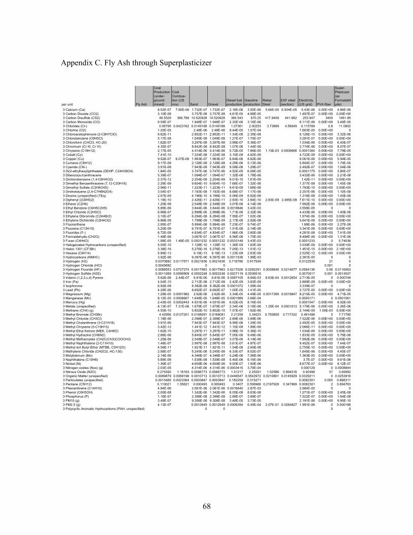
68
Appendix C. Fly Ash through Superplasticizer
3 Calcium (Ca) 8.52E-07 7.80E-06 1.732E-07 1.732E-07 2.18E-06 3.00E-06 5.66E-05 6.504E-05 5.43E-06 0.00E+00 4.86E-063 Carbon Dioxide (CO2) 3.10E-08 3.757E-08 3.757E-08 4.81E-05 4.88E-05 1.497E-07 0.00E+00 0.00E+003 Carbon Disulfide (CS2) 48.5529 366.768 10.520928 10.520928 385.543 670.25 417.9409 441.662 253.947 3400 1461.853 Carbon Monoxide (CO) 9.59E-07 1.948E-07 1.948E-07 2.35E-06 3.16E-06 6.111E-06 0.00E+00 3.49E-053 Chlorides (Cl-) 0.06795 0.0423162 0.0149188 0.0149188 1.07361 2.00253 3.73899 4.56849 0.115789 0.8 11.08023 Chlorine (Cl2) 1.20E-05 2.48E-06 2.48E-06 8.44E-05 1.57E-04 7.663E-05 0.00E+00 03 Chloroacetophenone (2-C8H7ClO) 9.82E-11 2.852E-11 2.852E-11 1.34E-08 2.35E-08 6.126E-10 0.00E+00 3.32E-063 Chlorobenzene (C6H5Cl) 5.17E-08 1.049E-08 1.049E-08 1.27E-07 1.70E-07 3.291E-07 0.00E+00 0.00E+003 Chloroform (CHCl3, HC-20) 1.62E-07 3.297E-08 3.297E-08 3.98E-07 5.36E-07 1.034E-06 0.00E+00 6.40E-073 Chromium (Cr III, Cr VI) 4.35E-07 8.842E-08 8.842E-08 1.07E-06 1.44E-06 2.774E-06 0.00E+00 8.07E-073 Chrysene (C18H12) 2.17E-05 4.414E-06 4.414E-06 5.72E-05 7.66E-05 1.13E-03 0.0008666 0.0001384 0.00E+00 7.79E-053 Cobalt (Co) 7.41E-10 7.224E-08 7.224E-08 3.15E-09 4.82E-09 4.722E-09 0.00E+00 0.00E+003 Copper (Cu) 9.52E-07 6.07E-06 1.963E-07 1.963E-07 6.84E-06 8.82E-06 6.061E-06 0.00E+00 5.94E-053 Cumene (C9H12) 9.17E-08 2.128E-08 2.128E-08 4.29E-06 5.13E-06 5.804E-07 0.00E+00 1.79E-053 Cyanide (CN-) 3.91E-08 7.943E-09 7.943E-09 9.58E-08 1.29E-07 2.492E-07 0.00E+00 1.04E-063 Di(2-ethylhexyl)phthalate (DEHP, C24H38O4) 1.84E-05 3.747E-06 3.747E-06 4.52E-05 6.09E-05 0.0001175 0.00E+00 3.80E-073 Dibenzo(a,h)anthracene 5.39E-07 1.094E-07 1.094E-07 1.32E-06 1.78E-06 3.432E-06 0.00E+00 2.21E-083 Dichlorobenzene (1,4-C6H4Cl2) 2.37E-12 2.254E-09 2.254E-09 9.01E-10 1.61E-09 1.42E-11 0.00E+00 0.00E+003 Dimethyl Benzanthracene (7,12-C20H16) 2.28E-09 9.604E-10 9.604E-10 7.68E-07 1.32E-06 1.377E-08 0.00E+00 1.45E-083 Dimethyl Sulfate (C2H6O4S) 2.96E-11 1.223E-11 1.223E-11 9.61E-09 1.66E-08 1.793E-10 0.00E+00 0.00E+003 Dinitrotoluene (2,4-C7H6N2O4) 3.54E-07 7.193E-08 7.193E-08 8.68E-07 1.17E-06 2.257E-06 0.00E+00 1.10E-083 Dioxins (unspecified) (TEq) 2.07E-09 4.196E-10 4.196E-10 5.06E-09 6.82E-09 1.316E-08 0.00E+00 1.40E-083 Diphenyl ((C6H5)2) 1.19E-10 2.426E-11 2.426E-11 2.93E-10 3.94E-10 2.83E-09 2.485E-09 7.611E-10 0.00E+00 0.00E+003 Ethane (C2H6) 1.25E-08 2.548E-09 2.548E-09 3.07E-08 4.14E-08 7.992E-08 0.00E+00 0.00E+003 Ethyl Benzene (C6H5C2H5) 5.89E-06 3.844E-06 3.844E-06 0.0019846 3.42E-03 3.558E-05 0 03 Ethyl Chloride (C2H5Cl) 6.96E-07 2.998E-06 2.998E-06 1.71E-06 2.32E-06 4.433E-06 0.00E+00 1.40E-063 Ethylene Dibromide (C2H4Br2) 3.10E-07 6.294E-08 6.294E-08 7.59E-07 1.02E-06 1.974E-06 0.00E+00 0.00E+003 Ethylene Dichloride (C2H4Cl2) 8.86E-09 1.798E-09 1.798E-09 2.17E-08 2.92E-08 5.641E-08 0.00E+00 0.00E+003 Fluoranthene 2.95E-07 5.994E-08 5.994E-08 7.23E-07 9.74E-07 1.88E-06 0.00E+00 2.27E-083 Fluorene (C13H10) 5.25E-09 6.791E-07 6.791E-07 1.51E-08 2.14E-08 3.341E-08 0.00E+00 0.00E+003 Fluorides (F-) 6.72E-09 4.834E-07 4.834E-07 1.86E-08 2.60E-08 4.281E-08 0.00E+00 7.41E-093 Formaldehyde (CH2O) 1.49E-06 3.067E-07 3.067E-07 9.56E-06 1.75E-05 9.494E-06 0.00E+00 1.31E-063 Furan (C4H4O) 1.99E-05 1.48E-05 0.0001232 0.0001232 0.0033148 3.43E-03 0.0001233 0 0.740363 Halogenated Hydrocarbons (unspecified) 5.55E-10 1.128E-10 1.128E-10 1.36E-09 1.83E-09 3.539E-09 0.00E+00 0.00E+003 Halon 1301 (CF3Br) 3.38E-16 5.276E-16 5.276E-16 7.05E-13 1.51E-12 1.451E-15 0.00E+00 2.16E+003 Hexane (C6H14) 5.89E-13 9.18E-13 9.18E-13 1.23E-09 2.63E-09 2.525E-12 0.00E+00 0.00E+003 Hydrocarbons (NMHC) 3.92E-06 9.397E-06 9.397E-06 0.0011536 1.99E-03 2.381E-05 0 03 Hydrogen (H2) 0.0370682 0.0117571 0.0021636 0.0021636 0.716786 0.917549 0.0122539 21 03 Hydrogen Chloride (HCl) 0.0045692 0 0 0.001 03 Hydrogen Fluoride (HF) 0.0088553 0.0727274 0.0017983 0.0017983 0.0217028 0.0292291 0.0038848 0.0214677 0.0564136 0.06 0.01160633 Hydrogen Sulfide (H2S) 0.0011069 0.0090909 0.0002248 0.0002248 0.0027119 0.0036516 0.0070517 0.001 0.00145073 Indeno (1,2,3,c,d) Pyrene 5.62E-06 2.44E-07 6.81E-06 6.81E-06 0.0087105 8.84E-03 8.63E-04 0.0012654 2.713E-05 0 0.0007483 Iron (Fe) 4.54E-10 2.712E-08 2.712E-08 2.42E-09 3.83E-09 2.889E-09 0.00E+00 0.00E+003 Isophorone 6.92E-08 8.382E-08 8.382E-08 0.0001072 1.09E-04 3.339E-07 0 03 Lead (Pb) 4.28E-06 8.692E-07 8.692E-07 1.05E-05 1.41E-05 2.727E-05 0.00E+00 0.00E+003 Magnesium (Mg) 1.29E-05 0.0001982 2.62E-06 2.62E-06 3.34E-05 4.49E-05 0.0017399 0.0019847 8.215E-05 0.00E+00 4.71E-053 Manganese (Mn) 8.12E-05 0.0006667 1.648E-05 1.648E-05 0.0001989 2.68E-04 0.0005171 0 0.00010613 Mercury (Hg) 2.43E-05 0.0002443 4.931E-06 4.931E-06 6.02E-05 8.16E-05 0.0001547 0.00E+00 6.92E-053 Metals (unspecified) 8.13E-07 7.31E-06 1.679E-07 1.679E-07 2.34E-06 3.18E-06 1.25E-04 0.0001013 5.179E-06 0.00E+00 2.26E-063 Methane (CH4) (g) 4.55E-10 5.852E-10 5.852E-10 7.57E-07 1.62E-06 2.144E-09 1.00E-03 0.00E+003 Methyl Bromide (CH3Br) 4.42956 0.0127201 0.0168091 0.0168091 2.21258 3.34023 0.750859 0.717332 0.481498 0 7.717853 Methyl Chloride (CH3Cl) 1.18E-06 2.398E-07 2.398E-07 2.89E-06 3.89E-06 7.522E-06 0.00E+00 0.00E+003 Methyl Cholanthrene (3-C21H16) 3.91E-06 7.943E-07 7.943E-07 9.58E-06 1.29E-05 2.492E-05 0.00E+00 0.00E+003 Methyl Chrysene (5-C19H15) 3.42E-12 1.441E-12 1.441E-12 1.15E-09 1.99E-09 2.066E-11 0.00E+00 0.00E+003 Methyl Ethyl Ketone (MEK, C4H8O) 1.62E-10 3.297E-11 3.297E-11 3.98E-10 5.36E-10 1.034E-09 0.00E+00 0.00E+003 Methyl Hydrazine (CH6N2) 2.88E-06 5.845E-07 5.845E-07 7.05E-06 9.49E-06 1.833E-05 0.00E+00 5.79E-063 Methyl Methacrylate (CH2C(CH3)COOCH3) 1.25E-06 2.548E-07 2.548E-07 3.07E-06 4.14E-06 7.992E-06 0.00E+00 0.00E+003 Methyl Naphthalene (2-C11H10) 1.48E-07 2.997E-08 2.997E-08 3.61E-07 4.87E-07 9.402E-07 0.00E+00 7.44E-073 Methyl tert Butyl Ether (MTBE, C5H12O) 4.56E-11 1.921E-11 1.921E-11 1.54E-08 2.65E-08 2.755E-10 0.00E+00 0.00E+003 Methylene Chloride (CH2Cl2, HC-130) 2.58E-07 5.245E-08 5.245E-08 6.33E-07 8.52E-07 1.645E-06 0.00E+00 4.45E-073 Molybdenum (Mo) 2.14E-06 4.346E-07 4.346E-07 5.24E-06 7.06E-06 1.363E-05 0.00E+00 0.00E+003 Naphthalene (C10H8) 5.89E-08 1.539E-08 1.539E-08 5.40E-06 6.16E-06 3.7E-07 0.00E+00 9.61E-063 Nickel (Ni) 1.36E-07 4.659E-06 4.659E-06 9.00E-07 1.50E-06 8.677E-07 0.00E+00 8.12E-073 Nitrogen oxides (Nox) (g) 2.03E-05 4.314E-06 4.314E-06 0.0003415 3.79E-04 0.000129 0 0.00088443 Nitrous Oxide (N2O) 0.275592 1.16163 0.0566773 0.0566773 1.51217 2.25591 1.02586 0.894316 0.92498 57 3.699923 Organic Matter (unspecified) 0.0089879 0.0069196 0.0010713 0.0010713 0.0446547 0.0542972 0.0210801 0.0145929 0.0329211 0 0.02539163 Particulates (unspecified) 0.0015485 0.0023364 0.0003847 0.0003847 0.182259 0.315271 0.0082301 0.005 0.8883113 Pentane (C5H12) 0.110021 1.55621 0.000493 0.000493 0.3407 0.506966 0.2197928 0.347969 0.0082301 2 0.6947633 Phenanthrene (C14H10) 4.94E-06 2.081E-06 2.081E-06 0.0016645 2.87E-03 2.984E-05 0 03 Phenol (C6H5OH) 2.00E-08 1.342E-06 1.342E-06 6.05E-08 8.63E-08 1.271E-07 0.00E+00 2.45E-083 Phosphorus (P) 1.18E-07 2.398E-08 2.398E-08 2.89E-07 3.89E-07 7.522E-07 0.00E+00 1.64E-063 PM10 (g) 3.49E-07 9.306E-08 9.306E-08 3.48E-05 3.73E-05 2.191E-06 0.00E+00 9.95E-103 PM2.5 (g) 4.13E-07 0.0012649 0.0012649 0.0006394 6.49E-04 2.07E-01 0.3284827 1.991E-06 0 0.0001883 Polycyclic Aromatic Hydrocarbons (PAH, unspecified) 0 0 0 0
per unit Fly Ash
Coal Production (under-ground mined)
Coal Combus-tion (US mix) Sand Gravel
Diesel fuel production
Gasoline production
Rebar Steel
EAF steel (section)
Electricity (US grid) PVA fiber
Super-Plastcizer (as Formaldehyde)
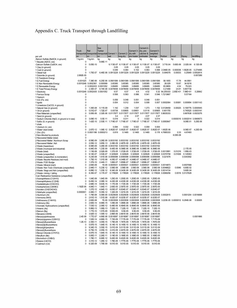
69
Appendix C. Truck Transport through Landfilling
Truck transportation
Rail transportation
Sea Tanker transportation
Cement 1 - wet
Cement 2- long-dry
Cement 3 - dry with pre-heater
Cement 4 - dry, pre-calciner & preheater
Cement 5 - weighted average Rubber wood Epoxy landfilling
1 kg-km 1 kg-km kg kg kg kg kg kg kg kg kg kg0 8.98E-110 5.05E-10 6.113E-07 6.113E-07 6.113E-07 6.113E-07 6.113E-07 3.71E-04 5.60E-06 2.02E-04 6.12E-080 0.05 0.05 0.05 0.05 0.050 0.049 0.064 0.102 0.063 0.068 2.046E-05 0.000036 1.562E-05 0.2744950 1.70E-07 6.46E-08 0.0913229 0.0913229 0.0913229 0.0913229 0.0913229 0.094078 0.00033 0.25949 0.0002814
2.892E-05 0.0072890
-0.001025 7.38E-06 6.25E-06 0.0901589 0.0901589 0.0901589 0.0901589 0.0901589 58.1855 17.78 44.95610.0010248 0.0002361 0.000099 3.65385 3.65385 3.65385 3.65385 3.65385 26.029 10.67 34.9216
0 0.0002433 0.0001052 3.69485 3.69485 3.69485 3.69485 3.69485 83.9855 4.54 79.0230 2.30E-07 8.74E-08 0.0478058 0.0478058 0.0478058 0.0478058 0.0478058 0.21468 23.91 0.857736
0.0010248 0.0002435 0.0001052 6.57 6.07 4.9 4.52 5.32 84.200333 2.85E+01 7.99E+01 0.268420 0.506 0.563 0.586 0.541 0.546 1.7213667 5.5716400 0.059 0.048 0.051 0.048 0.0510 0.004 0.012 0.004 0.008 0.007 0.0002084 0.00081 0.000694 0.000114300 1.35E-08 5.11E-09 1.142 1.239 1.037 1.273 1.192 0.0128459 0.00025 0.190776 0.00005450 5.51E-07 1.72E-07 0.00738 0.00805 0.00651 0.0116 0.00905 0.901755 0.745525 0.00031910 5.00E-06 2.32E-06 0.0117877 0.0117877 0.0117877 0.0117877 0.0117877 0.8635333 0.667638 0.00232760 3.4 2.14 2.07 2.07 2.370 3.09E-10 5.5E-11 0.019 0.011 0 0.022 0.014 0.0000016 0.0002014 0.09095730 1.42E-10 2.53E-11 1.719E-07 1.719E-07 1.719E-07 1.719E-07 1.719E-07 0.0063647 9.09E-01 5.25E-0600 0.094 0.032 0.022 0.059 0.0540 2.87E-12 1.09E-12 5.952E-07 5.952E-07 5.952E-07 5.952E-07 5.952E-07 1.802E-06 8.56E-07 4.20E-090 0.0001186 0.0000213 0.819 0.1465 0.1465 0.1465 0.176 4.7685333 0.33 4.674930 6.00E-0800 8.58E-09 3.26E-09 0.0033192 0.0033192 0.0033192 0.0033192 0.00331920 2.05E-12 3.65E-13 2.49E-09 2.487E-09 2.487E-09 2.487E-09 2.487E-090 8.58E-09 3.26E-09 0.0033192 0.0033192 0.0033192 0.0033192 0.00331920 6.94E-09 1.23E-09 8.40E-06 8.398E-06 8.398E-06 8.398E-06 8.398E-06 2.17E-050 1.13E-08 2.02E-09 1.37E-05 1.372E-05 1.372E-05 1.372E-05 1.372E-05 0.0013991 0.01216 1.95E-030 9.14E-07 3.53E-07 0.320628 0.320628 0.320628 0.320628 0.320628 0.0370758 0.01836 0.1293630 4.23E-08 1.61E-08 0.0090098 0.0090098 0.0090098 0.0090098 0.0090098 0.021678 0.03430920 1.75E-10 1.01E-08 4.05E-07 4.048E-07 4.048E-07 4.048E-07 4.048E-070 1.37E-10 2.44E-11 1.66E-07 1.659E-07 1.659E-07 1.659E-07 1.659E-070 2.65E-09 1E-09 0.0005531 0.0005531 0.0005531 0.0005531 0.0005531 0.0014873 0.00070680 2.94E-11 5.23E-12 3.56E-08 3.56E-08 3.56E-08 3.56E-08 3.56E-08 0.0048622 0.0046 6.80E-020 6.89E-12 1.23E-12 8.34E-09 8.343E-09 8.343E-09 8.343E-09 8.343E-09 0.0014134 5.60E-040 8.35E-07 3.17E-07 0.178028 0.178028 0.178028 0.178028 0.178028 0.0069256 0.0016 0.013762800 1.04E-08 1.84E-09 1.25E-05 1.255E-05 1.255E-05 1.255E-05 1.255E-050 6.45E-14 2.08E-14 4.43E-08 4.433E-08 4.433E-08 4.433E-08 4.433E-080 2.68E-14 9.63E-15 1.17E-08 1.172E-08 1.172E-08 1.172E-08 1.172E-08
1.192E-06 4.84E-11 1.84E-11 2.60E-05 2.597E-05 2.597E-05 2.597E-05 2.597E-050 1.27E-12 4.84E-13 6.83E-07 6.834E-07 6.834E-07 6.834E-07 6.834E-07
0.0000001 2.46E-11 9.35E-12 1.32E-05 1.321E-05 1.321E-05 1.321E-05 1.321E-050 1.79E-08 5.08E-09 0.0025638 0.0025638 0.0025638 0.0025638 0.0025638 0.0002815 0.0001204 0.00166990 2.61E-10 1.51E-08 6.02E-07 6.023E-07 6.023E-07 6.023E-07 6.023E-070 2.60E-08 7E-09 0.0003938 0.0003938 0.0003938 0.0003938 0.0003938 3.223E-05 0.0000012 8.294E-06 0.000050 2.60E-14 8.98E-15 1.09E-08 1.089E-08 1.089E-08 1.089E-08 1.089E-080 7.53E-12 2.08E-12 6.48E-06 6.484E-06 6.484E-06 6.484E-06 6.484E-060 5.96E-13 1.06E-13 7.22E-10 7.22E-10 7.22E-10 7.22E-10 7.22E-100 1.77E-10 1.57E-09 9.50E-05 9.5E-05 9.5E-05 9.5E-05 9.5E-050 3.92E-12 1.05E-12 2.86E-06 2.861E-06 2.861E-06 2.861E-06 2.861E-06
2.4E-08 1.77E-07 4.89E-08 0.0018087 0.0018087 0.0018087 0.0018087 0.0018087 0.00018660 1.52E-14 4.66E-15 7.72E-09 7.717E-09 7.717E-09 7.717E-09 7.717E-09
1.2E-10 2.35E-11 3.05E-15 1.79E-09 1.787E-09 1.787E-09 1.787E-09 1.787E-090 5.97E-15 1.64E-15 8.14E-10 8.145E-10 8.145E-10 8.145E-10 8.145E-100 9.34E-15 3.55E-15 5.01E-09 5.011E-09 5.011E-09 5.011E-09 5.011E-090 6.75E-15 2.05E-15 2.41E-09 2.407E-09 2.407E-09 2.407E-09 2.407E-090 5.97E-15 1.64E-15 8.14E-10 8.145E-10 8.145E-10 8.145E-10 8.145E-100 5.95E-11 2.26E-11 3.19E-05 3.189E-05 3.189E-05 3.189E-05 3.189E-050 1.78E-11 6.68E-12 9.40E-06 9.402E-06 9.402E-06 9.402E-06 9.402E-060 3.31E-12 1.26E-12 1.78E-06 1.777E-06 1.777E-06 1.777E-06 1.777E-060 6.32E-09 1.79E-09 9.01E-05 9.01E-05 9.01E-05 9.01E-05 9.01E-05
per unit1 Barium Sulfate (BaSO4, in ground)1 Bauxite (Al2O3, ore) 1 Calcium Sulfate (CaSO4, ore)1 Clay (in ground)1 Coal (in ground)1 Diesel fuel1 Dolomite (in ground)1 E Feedstock Energy1 E Fuel Energy1 E Non Renewable Energy1 E Renewable Energy1 E Total Primary Energy1 Electricity1 Ferrous Scrap1 Gypsum1 Iron (Fe, ore)1 lignite1 Limestone (CaCO3, in ground)1 Natural Gas (in ground)1 Oil (in ground)1 Raw Materials (unspecified)1 Sand (in ground)1 Sodium Chloride (NaCl, in ground or in sea)1 Sulfur (S, in ground)1 shale1 Uranium (U, ore)1 Water Used (total)1 Zinc (Zn)2 Non-Allocted by products2 Recovered Matter (total)2 Recovered Matter: Aluminum Scrap2 Recovered Matter: Ash2 Waste (hazardous)2 Waste (municipal and industrial)2 Waste (total)2 Waste (unspecified)2 Waste (unspecified, to incineration)2 Waste: Bauxite Residues (red mud)2 Waste: FGD Sludge2 Waste: Mineral (inert)2 Waste: Non Toxic Chemicals (unspecified)2 Waste: Slags and Ash (unspecified)2 Waste: mining + tailing3 (ar) Radioactive Substance (unspecified)3 Acenaphthene (C12H10)3 Acenaphthylene (C12H8)3 Acetaldehyde (CH3CHO)3 Acetophenone (C8H8O)3 Acrolein (CH2CHCHO)3 Aldehyde (unspecified)3 Aluminum (Al)3 Ammonia (NH3)3 Anthracene (C14H10)3 Antimony (Sb)3 Aromatic Hydrocarbons (unspecified)3 Arsenic (As)3 Barium (Ba)3 Benzene (C6H6)3 Benzo(a)anthracene3 Benzo(a)pyrene (C20H12)3 Benzo(b)fluoranthene3 Benzo(bjk)fluoranthene3 Benzo(ghi)perylene3 Benzo(k)fluoranthene3 Benzyl Chloride (C7H7Cl)3 Beryllium (Be)3 Bromoform (CHBr3)3 Butane (C4H10)3 Cadmium (Cd)
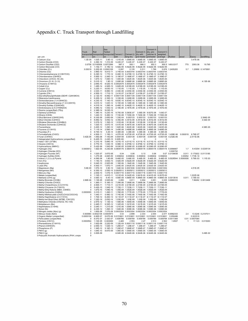
70
Appendix C. Truck Transport through Landfilling
3 Calcium (Ca) 1.3E-09 1.02E-11 3.8E-12 1.01E-05 1.006E-05 1.006E-05 1.006E-05 1.006E-05 3.47E-063 Carbon Dioxide (CO2) 0 2.26E-10 1.31E-08 5.22E-07 5.22E-07 5.22E-07 5.22E-07 5.22E-073 Carbon Disulfide (CS2) 0.0756 0.0165936 0.0072599 997.3 930.1 866.3 852.3 900.5 1493.0317 770 2093.38 19.7853 Carbon Monoxide (CO) 0 1.10E-11 4.19E-12 5.92E-06 5.922E-06 5.922E-06 5.922E-06 5.922E-063 Chlorides (Cl-) 0.00019 5.20E-05 0.0000128 0.097 0.135 0.511 1.799 0.876 1.2405283 5.7 1.25666 0.14758913 Chlorine (Cl2) 0 3.96E-10 9.91E-11 3.74E-04 0.0003744 0.0003744 0.0003744 0.00037443 Chloroacetophenone (2-C8H7ClO) 0 6.29E-14 1.77E-14 6.48E-10 6.479E-10 6.479E-10 6.479E-10 6.479E-103 Chlorobenzene (C6H5Cl) 0 5.95E-13 2.26E-13 3.19E-07 3.189E-07 3.189E-07 3.189E-07 3.189E-073 Chloroform (CHCl3, HC-20) 0 1.87E-12 7.09E-13 1.00E-06 1.002E-06 1.002E-06 1.002E-06 1.002E-063 Chromium (Cr III, Cr VI) 0 5.01E-12 1.9E-12 2.69E-06 2.688E-06 2.688E-06 2.688E-06 2.688E-06 4.13E-063 Chrysene (C18H12) 0 2.69E-10 8.52E-10 0.0002478 0.0002478 0.0002478 0.0002478 0.00024783 Cobalt (Co) 0 1.48E-14 4.92E-15 5.82E-09 5.818E-09 5.818E-09 5.818E-09 5.818E-093 Copper (Cu) 0 3.22E-11 9.63E-10 1.11E-05 1.11E-05 1.11E-05 1.11E-05 1.11E-053 Cumene (C9H12) 0 2.02E-11 8.88E-10 2.04E-06 2.035E-06 2.035E-06 2.035E-06 2.035E-063 Cyanide (CN-) 0 4.50E-13 1.71E-13 2.41E-07 2.415E-07 2.415E-07 2.415E-07 2.415E-073 Di(2-ethylhexyl)phthalate (DEHP, C24H38O4) 0 2.12E-10 8.06E-11 0.0001139 0.0001139 0.0001139 0.0001139 0.00011393 Dibenzo(a,h)anthracene 0 6.20E-12 2.35E-12 3.33E-06 3.326E-06 3.326E-06 3.326E-06 3.326E-063 Dichlorobenzene (1,4-C6H4Cl2) 0 4.23E-15 1.14E-15 8.83E-10 8.834E-10 8.834E-10 8.834E-10 8.834E-103 Dimethyl Benzanthracene (7,12-C20H16) 0 3.61E-12 1.02E-12 5.15E-08 5.148E-08 5.148E-08 5.148E-08 5.148E-083 Dimethyl Sulfate (C2H6O4S) 0 4.51E-14 1.28E-14 6.46E-10 6.462E-10 6.462E-10 6.462E-10 6.462E-103 Dinitrotoluene (2,4-C7H6N2O4) 0 4.08E-12 1.55E-12 2.19E-06 2.187E-06 2.187E-06 2.187E-06 2.187E-063 Dioxins (unspecified) (TEq) 0 2.38E-14 9.03E-153 Diphenyl ((C6H5)2) 0 1.38E-15 5.22E-16 9.75E-08 5.583E-07 3.56E-09 9.927E-08 1.64E-073 Ethane (C2H6) 0 1.44E-13 5.48E-14 7.74E-08 7.745E-08 7.745E-08 7.745E-08 7.745E-083 Ethyl Benzene (C6H5C2H5) 0 9.33E-09 2.65E-09 1.33E-04 0.000133 0.000133 0.000133 0.000133 2.384E-053 Ethyl Chloride (C2H5Cl) 0 8.06E-12 3.05E-12 4.35E-06 4.351E-06 4.351E-06 4.351E-06 4.351E-06 4.52E-043 Ethylene Dibromide (C2H4Br2) 0 3.57E-12 1.35E-12 1.91E-06 1.913E-06 1.913E-06 1.913E-06 1.913E-063 Ethylene Dichloride (C2H4Cl2) 0 1.02E-13 3.87E-14 5.47E-08 5.467E-08 5.467E-08 5.467E-08 5.467E-083 Fluoranthene 0 3.40E-12 1.29E-12 1.82E-06 1.822E-06 1.822E-06 1.822E-06 1.822E-06 4.58E-053 Fluorene (C13H10) 0 7.11E-14 2.58E-14 3.49E-08 3.489E-08 3.489E-08 3.489E-08 3.489E-083 Fluorides (F-) 0 8.74E-14 3.2E-14 4.38E-08 4.38E-08 4.38E-08 4.38E-08 4.38E-083 Formaldehyde (CH2O) 0 4.50E-11 1.15E-11 4.07E-05 4.072E-05 4.072E-05 4.072E-05 4.072E-05 1.428E-06 0.000018 6.78E-073 Furan (C4H4O) 3.42E-06 1.56E-08 7.14E-09 0.000138 0.000138 0.000138 0.000138 0.000138 4.232E-06 2.011E-063 Halogenated Hydrocarbons (unspecified) 0 6.40E-15 2.43E-15 0.00E+00 0 0 0 03 Halon 1301 (CF3Br) 0 3.31E-18 5.89E-19 4.01E-15 4.011E-15 4.011E-15 4.011E-15 4.011E-153 Hexane (C6H14) 0 5.77E-15 1.03E-15 6.98E-12 6.979E-12 6.979E-12 6.979E-12 6.979E-123 Hydrocarbons (NMHC) 0 5.42E-09 1.54E-09 8.03E-05 8.028E-05 8.028E-05 8.028E-05 8.028E-053 Hydrogen (H2) 0.0000912 1.92E-05 4.23E-06 0.0809178 0.0809178 0.0809178 0.0809178 0.0809178 5.0066667 1.7 8.43204 0.02261343 Hydrogen Chloride (HCl) 0 0.0007523 Hydrogen Fluoride (HF) 0 1.02E-07 3.87E-08 0.04 0.06 0.13 0.06 0.07 0.0109838 0.011 0.175922 0.01131853 Hydrogen Sulfide (H2S) 0 1.27E-08 4.84E-09 0.006834 0.006834 0.006834 0.006834 0.006834 0.00052 1.173E-103 Indeno (1,2,3,c,d) Pyrene 0 4.09E-08 1.9E-08 9.46E-05 9.46E-05 9.46E-05 9.46E-05 9.46E-05 0.0028544 0.0000008 5.76E-03 1.11E-033 Iron (Fe) 0 1.14E-14 3.65E-15 3.92E-09 3.922E-09 3.922E-09 3.922E-09 3.922E-093 Isophorone 0 5.04E-10 2.92E-08 1.16E-06 1.164E-06 1.164E-06 1.164E-06 1.164E-063 Lead (Pb) 0 4.93E-11 1.87E-11 2.64E-05 2.642E-05 2.642E-05 2.642E-05 2.642E-053 Magnesium (Mg) 5.8E-09 1.57E-10 3.9E-10 1.84E-04 0.0001836 0.0001836 0.0001836 0.0001836 4.51E-053 Manganese (Mn) 0 9.35E-10 3.55E-10 0.0005012 0.0005012 0.0005012 0.0005012 0.00050123 Mercury (Hg) 0 2.83E-10 1.07E-10 0.0001716 0.0001716 0.0001716 0.0001716 0.00017163 Metals (unspecified) 0 1.10E-11 4.81E-11 5.51E-05 8.342E-05 2.691E-05 6.941E-05 6.057E-05 1.222E-063 Methane (CH4) (g) 0 3.56E-12 6.4E-13 4.89E-09 4.886E-09 4.886E-09 4.886E-09 4.886E-09 0.0013616 0.011 3.18E-033 Methyl Bromide (CH3Br) 2.88E-06 1.13E-05 3.52E-06 0.055 0.011 0.004 0.051 0.035 3.6969333 7.86262 0.00124063 Methyl Chloride (CH3Cl) 0 1.36E-11 5.16E-12 7.29E-06 7.289E-06 7.289E-06 7.289E-06 7.289E-063 Methyl Cholanthrene (3-C21H16) 0 4.50E-11 1.71E-11 2.41E-05 2.415E-05 2.415E-05 2.415E-05 2.415E-053 Methyl Chrysene (5-C19H15) 0 5.42E-15 1.54E-15 7.72E-11 7.723E-11 7.723E-11 7.723E-11 7.723E-113 Methyl Ethyl Ketone (MEK, C4H8O) 0 1.87E-15 7.09E-16 1.00E-09 1.002E-09 1.002E-09 1.002E-09 1.002E-093 Methyl Hydrazine (CH6N2) 0.0000005 3.31E-11 1.26E-11 1.78E-05 1.777E-05 1.777E-05 1.777E-05 1.777E-053 Methyl Methacrylate (CH2C(CH3)COOCH3) 0 1.44E-11 5.48E-12 7.74E-06 7.745E-06 7.745E-06 7.745E-06 7.745E-063 Methyl Naphthalene (2-C11H10) 0 1.70E-12 6.45E-13 9.11E-07 9.111E-07 9.111E-07 9.111E-07 9.111E-073 Methyl tert Butyl Ether (MTBE, C5H12O) 0 7.22E-14 2.05E-14 1.03E-09 1.03E-09 1.03E-09 1.03E-09 1.03E-093 Methylene Chloride (CH2Cl2, HC-130) 0 2.97E-12 1.13E-12 1.59E-06 1.594E-06 1.594E-06 1.594E-06 1.594E-063 Molybdenum (Mo) 0 2.46E-11 9.35E-12 1.32E-05 1.321E-05 1.321E-05 1.321E-05 1.321E-053 Naphthalene (C10H8) 0 2.54E-11 1.21E-09 1.01E-06 1.008E-06 1.008E-06 1.008E-06 1.008E-063 Nickel (Ni) 0 4.23E-12 1.26E-12 1.84E-06 1.838E-06 1.838E-06 1.838E-06 1.838E-063 Nitrogen oxides (Nox) (g) 0 1.60E-09 7.57E-08 0.0003354 0.0003354 0.0003354 0.0003354 0.00033543 Nitrous Oxide (N2O) 0.000984 0.0002139 0.0000973 3.53 2.898 2.333 2.044 2.577 8.6982333 2.4 13.0246 0.21075113 Organic Matter (unspecified) 0.0000106 6.80E-07 8.67E-08 0.0153601 0.0153601 0.0153601 0.0153601 0.0153601 0.050488 0.0225153 Particulates (unspecified) 0 8.57E-07 2.42E-07 0.008789 0.008789 0.008789 0.008789 0.008789 0.0017369 0.01 0.00070843 Pentane (C5H12) 0.0000504 1.10E-05 0.000006 2.465 2.553 2.47 2.513 2.502 1.8507 1 17.123 0.0152633 Phenanthrene (C14H10) 0 7.82E-09 2.22E-09 1.12E-04 0.0001116 0.0001116 0.0001116 0.00011163 Phenol (C6H5OH) 0 2.84E-13 1.02E-13 1.29E-07 1.29E-07 1.29E-07 1.29E-07 1.29E-073 Phosphorus (P) 0 1.36E-12 5.16E-13 7.29E-07 7.289E-07 7.289E-07 7.289E-07 7.289E-073 PM10 (g) 0 1.64E-10 8.87E-09 1.06E-05 1.056E-05 1.056E-05 1.056E-05 1.056E-053 PM2.5 (g) 0 3.00E-09 6.94E-06 6.944E-06 6.944E-06 6.944E-06 6.944E-06 3.49E-023 Polycyclic Aromatic Hydrocarbons (PAH, unspe 0
per unit
Truck transportation
Rail transportation
Sea Tanker transportation
Cement 1 - wet
Cement 2- long-dry
Cement 3 - dry with pre-heater
Cement 4 - dry, pre-calciner & preheater
Cement 5 - weighted average Rubber wood Epoxy landfilling
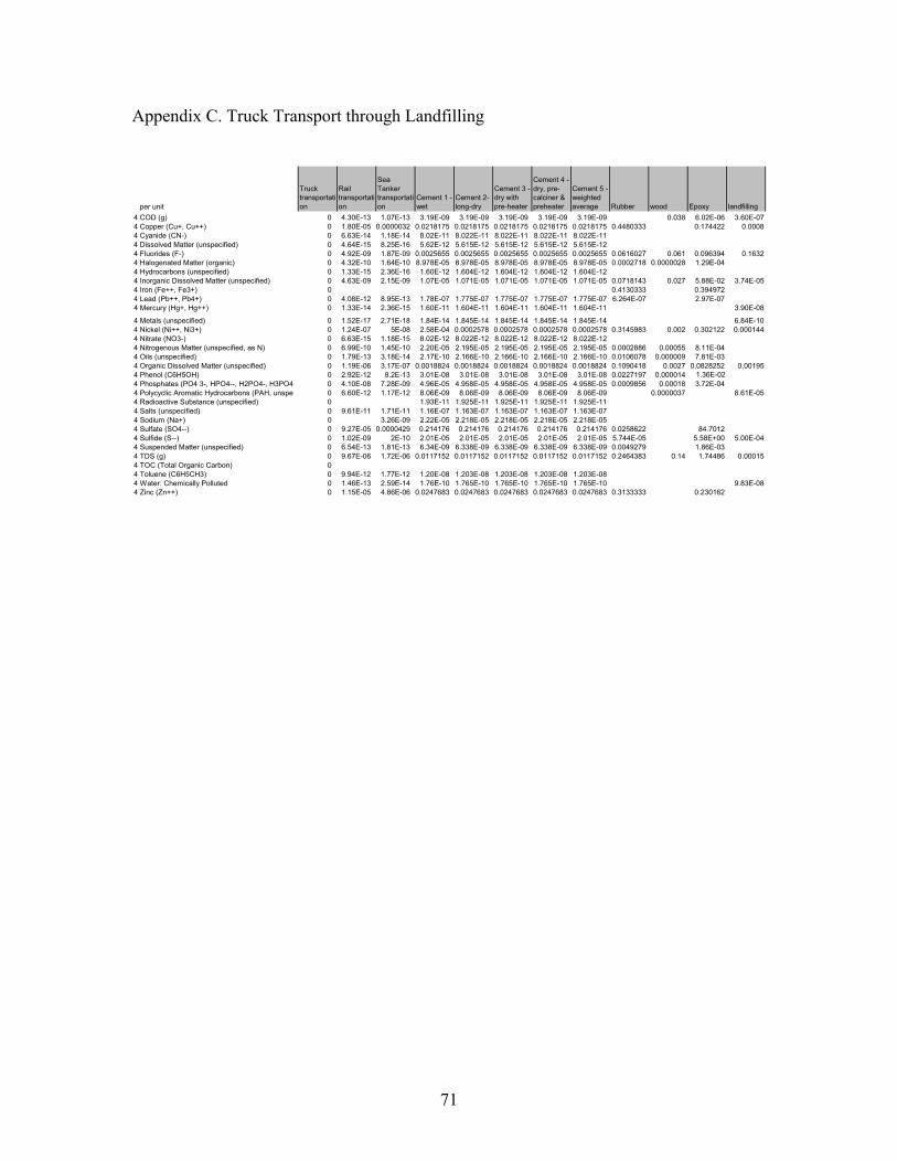
71
Appendix C. Truck Transport through Landfilling
4 COD (g) 0 4.30E-13 1.07E-13 3.19E-09 3.19E-09 3.19E-09 3.19E-09 3.19E-09 0.038 6.02E-06 3.60E-074 Copper (Cu+, Cu++) 0 1.80E-05 0.0000032 0.0218175 0.0218175 0.0218175 0.0218175 0.0218175 0.4480333 0.174422 0.00084 Cyanide (CN-) 0 6.63E-14 1.18E-14 8.02E-11 8.022E-11 8.022E-11 8.022E-11 8.022E-114 Dissolved Matter (unspecified) 0 4.64E-15 8.25E-16 5.62E-12 5.615E-12 5.615E-12 5.615E-12 5.615E-124 Fluorides (F-) 0 4.92E-09 1.87E-09 0.0025655 0.0025655 0.0025655 0.0025655 0.0025655 0.0616027 0.061 0.096394 0.16324 Halogenated Matter (organic) 0 4.32E-10 1.64E-10 8.978E-05 8.978E-05 8.978E-05 8.978E-05 8.978E-05 0.0002718 0.0000028 1.29E-044 Hydrocarbons (unspecified) 0 1.33E-15 2.36E-16 1.60E-12 1.604E-12 1.604E-12 1.604E-12 1.604E-124 Inorganic Dissolved Matter (unspecified) 0 4.63E-09 2.15E-09 1.07E-05 1.071E-05 1.071E-05 1.071E-05 1.071E-05 0.0718143 0.027 5.88E-02 3.74E-054 Iron (Fe++, Fe3+) 0 0.4130333 0.3949724 Lead (Pb++, Pb4+) 0 4.08E-12 8.95E-13 1.78E-07 1.775E-07 1.775E-07 1.775E-07 1.775E-07 6.264E-07 2.97E-074 Mercury (Hg+, Hg++) 0 1.33E-14 2.36E-15 1.60E-11 1.604E-11 1.604E-11 1.604E-11 1.604E-11 3.90E-08
4 Metals (unspecified) 0 1.52E-17 2.71E-18 1.84E-14 1.845E-14 1.845E-14 1.845E-14 1.845E-14 6.84E-104 Nickel (Ni++, Ni3+) 0 1.24E-07 5E-08 2.58E-04 0.0002578 0.0002578 0.0002578 0.0002578 0.3145983 0.002 0.302122 0.0001444 Nitrate (NO3-) 0 6.63E-15 1.18E-15 8.02E-12 8.022E-12 8.022E-12 8.022E-12 8.022E-124 Nitrogenous Matter (unspecified, as N) 0 6.99E-10 1.45E-10 2.20E-05 2.195E-05 2.195E-05 2.195E-05 2.195E-05 0.0002886 0.00055 8.11E-044 Oils (unspecified) 0 1.79E-13 3.18E-14 2.17E-10 2.166E-10 2.166E-10 2.166E-10 2.166E-10 0.0106078 0.000009 7.81E-034 Organic Dissolved Matter (unspecified) 0 1.19E-06 3.17E-07 0.0018824 0.0018824 0.0018824 0.0018824 0.0018824 0.1090418 0.0027 0.0828252 0.001954 Phenol (C6H5OH) 0 2.92E-12 8.2E-13 3.01E-08 3.01E-08 3.01E-08 3.01E-08 3.01E-08 0.0227197 0.000014 1.36E-024 Phosphates (PO4 3-, HPO4--, H2PO4-, H3PO4 0 4.10E-08 7.28E-09 4.96E-05 4.958E-05 4.958E-05 4.958E-05 4.958E-05 0.0009856 0.00018 3.72E-044 Polycyclic Aromatic Hydrocarbons (PAH, unspe 0 6.60E-12 1.17E-12 8.06E-09 8.06E-09 8.06E-09 8.06E-09 8.06E-09 0.0000037 8.61E-054 Radioactive Substance (unspecified) 0 1.93E-11 1.925E-11 1.925E-11 1.925E-11 1.925E-114 Salts (unspecified) 0 9.61E-11 1.71E-11 1.16E-07 1.163E-07 1.163E-07 1.163E-07 1.163E-074 Sodium (Na+) 0 3.26E-09 2.22E-05 2.218E-05 2.218E-05 2.218E-05 2.218E-054 Sulfate (SO4--) 0 9.27E-05 0.0000429 0.214176 0.214176 0.214176 0.214176 0.214176 0.0258622 84.70124 Sulfide (S--) 0 1.02E-09 2E-10 2.01E-05 2.01E-05 2.01E-05 2.01E-05 2.01E-05 5.744E-05 5.58E+00 5.00E-044 Suspended Matter (unspecified) 0 6.54E-13 1.81E-13 6.34E-09 6.338E-09 6.338E-09 6.338E-09 6.338E-09 0.0049279 1.86E-034 TDS (g) 0 9.67E-06 1.72E-06 0.0117152 0.0117152 0.0117152 0.0117152 0.0117152 0.2464383 0.14 1.74486 0.000154 TOC (Total Organic Carbon) 04 Toluene (C6H5CH3) 0 9.94E-12 1.77E-12 1.20E-08 1.203E-08 1.203E-08 1.203E-08 1.203E-084 Water: Chemically Polluted 0 1.46E-13 2.59E-14 1.76E-10 1.765E-10 1.765E-10 1.765E-10 1.765E-10 9.83E-084 Zinc (Zn++) 0 1.15E-05 4.86E-06 0.0247683 0.0247683 0.0247683 0.0247683 0.0247683 0.3133333 0.230162
per unit
Truck transportation
Rail transportation
Sea Tanker transportation
Cement 1 - wet
Cement 2- long-dry
Cement 3 - dry with pre-heater
Cement 4 - dry, pre-calciner & preheater
Cement 5 - weighted average Rubber wood Epoxy landfilling
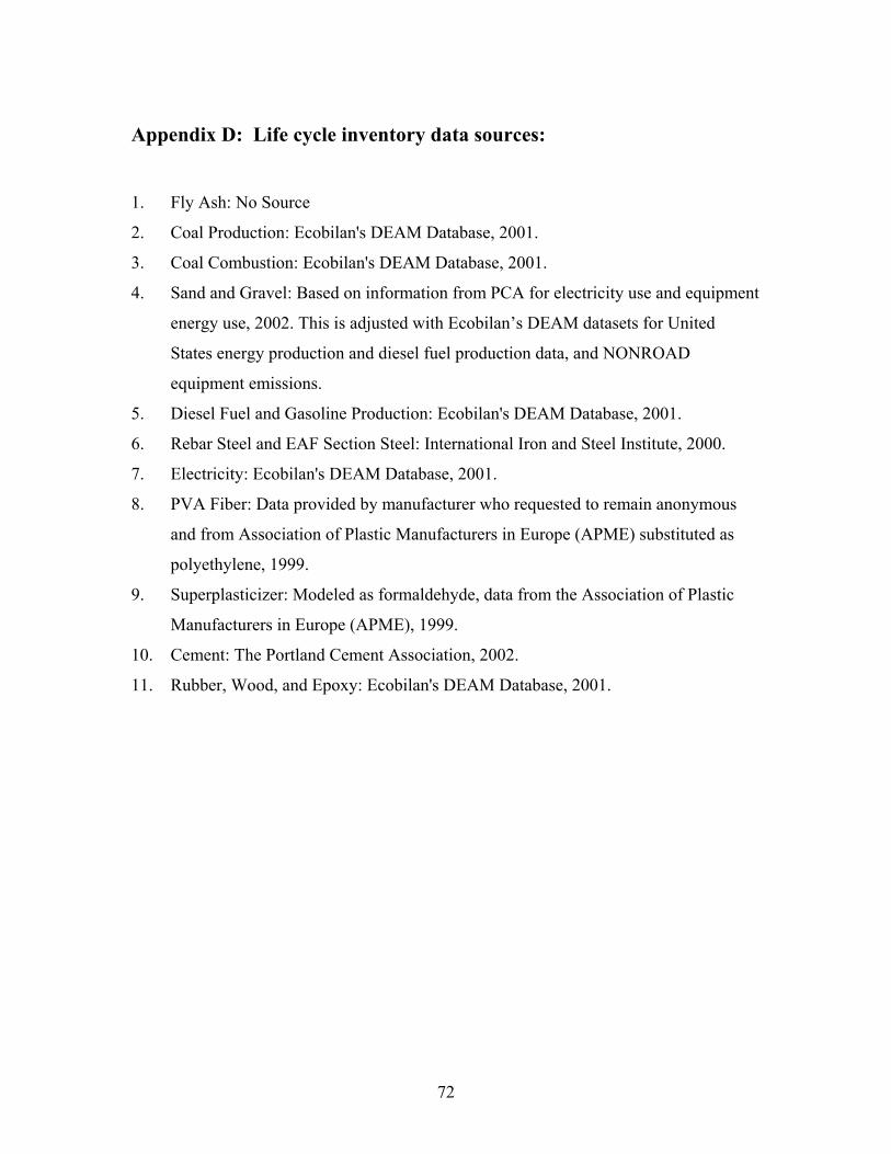
72
Appendix D: Life cycle inventory data sources:
1. Fly Ash: No Source
2. Coal Production: Ecobilan's DEAM Database, 2001.
3. Coal Combustion: Ecobilan's DEAM Database, 2001.
4. Sand and Gravel: Based on information from PCA for electricity use and equipment
energy use, 2002. This is adjusted with Ecobilan’s DEAM datasets for United
States energy production and diesel fuel production data, and NONROAD
equipment emissions.
5. Diesel Fuel and Gasoline Production: Ecobilan's DEAM Database, 2001.
6. Rebar Steel and EAF Section Steel: International Iron and Steel Institute, 2000.
7. Electricity: Ecobilan's DEAM Database, 2001.
8. PVA Fiber: Data provided by manufacturer who requested to remain anonymous
and from Association of Plastic Manufacturers in Europe (APME) substituted as
polyethylene, 1999.
9. Superplasticizer: Modeled as formaldehyde, data from the Association of Plastic
Manufacturers in Europe (APME), 1999.
10. Cement: The Portland Cement Association, 2002.
11. Rubber, Wood, and Epoxy: Ecobilan's DEAM Database, 2001.
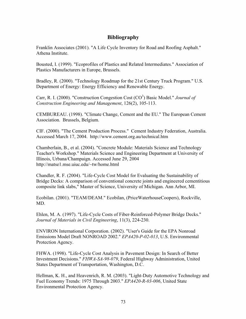
73
Bibliography
Franklin Associates (2001). "A Life Cycle Inventory for Road and Roofing Asphalt." Athena Institute.
Bousted, I. (1999). "Ecoprofiles of Plastics and Related Intermediates." Association of Plastics Manufacturers in Europe, Brussels.
Bradley, R. (2000). "Technology Roadmap for the 21st Century Truck Program." U.S. Department of Energy: Energy Efficiency and Renewable Energy.
Carr, R. I. (2000). "Construction Congestion Cost (CO3) Basic Model." Journal of Construction Engineering and Management, 126(2), 105-113.
CEMBUREAU. (1998). "Climate Change, Cement and the EU." The European Cement Association. Brussels, Belgium.
CIF. (2000). "The Cement Production Process." Cement Industry Federation, Australia. Accessed March 17, 2004. http://www.cement.org.au/technical.htm
Chamberlain, B., et al. (2004). "Concrete Module: Materials Science and Technology Teacher's Workshop." Materials Science and Engineering Department at University of Illinois, Urbana/Champaign. Accessed June 29, 2004 http://matse1.mse.uiuc.edu/~tw/home.html
Chandler, R. F. (2004). "Life-Cycle Cost Model for Evaluating the Sustainability of Bridge Decks: A comparison of conventional concrete joints and engineered cementitious composite link slabs," Master of Science, University of Michigan. Ann Arbor, MI. Ecobilan. (2001). "TEAM/DEAM." Ecobilan, (PriceWaterhouseCoopers), Rockville, MD. Ehlen, M. A. (1997). "Life-Cycle Costs of Fiber-Reinforced-Polymer Bridge Decks." Journal of Materials in Civil Engineering, 11(3), 224-230.
ENVIRON International Corporation. (2002). "User's Guide for the EPA Nonroad Emissions Model Draft NONROAD 2002." EPA420-P-02-013, U.S. Environmental Protection Agency. FHWA. (1998). "Life-Cycle Cost Analysis in Pavement Design: In Search of Better Investment Decisions." FHWA-SA-98-079, Federal Highway Administration, United States Department of Transportation, Washington, D.C. Hellman, K. H., and Heavenrich, R. M. (2003). "Light-Duty Automotive Technology and Fuel Economy Trends: 1975 Through 2003." EPA420-R-03-006, United State Environmental Protection Agency.
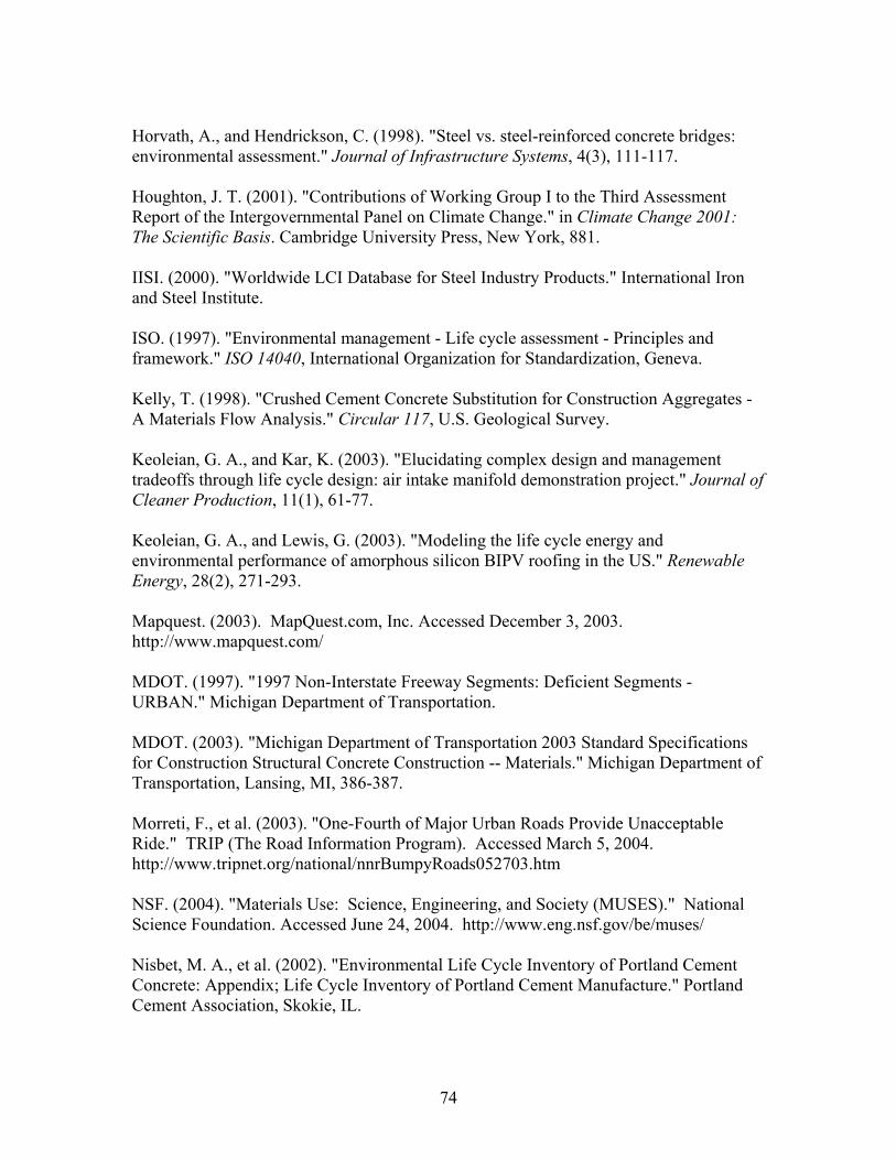
74
Horvath, A., and Hendrickson, C. (1998). "Steel vs. steel-reinforced concrete bridges: environmental assessment." Journal of Infrastructure Systems, 4(3), 111-117. Houghton, J. T. (2001). "Contributions of Working Group I to the Third Assessment Report of the Intergovernmental Panel on Climate Change." in Climate Change 2001: The Scientific Basis. Cambridge University Press, New York, 881. IISI. (2000). "Worldwide LCI Database for Steel Industry Products." International Iron and Steel Institute. ISO. (1997). "Environmental management - Life cycle assessment - Principles and framework." ISO 14040, International Organization for Standardization, Geneva. Kelly, T. (1998). "Crushed Cement Concrete Substitution for Construction Aggregates - A Materials Flow Analysis." Circular 117, U.S. Geological Survey. Keoleian, G. A., and Kar, K. (2003). "Elucidating complex design and management tradeoffs through life cycle design: air intake manifold demonstration project." Journal of Cleaner Production, 11(1), 61-77.
Keoleian, G. A., and Lewis, G. (2003). "Modeling the life cycle energy and environmental performance of amorphous silicon BIPV roofing in the US." Renewable Energy, 28(2), 271-293. Mapquest. (2003). MapQuest.com, Inc. Accessed December 3, 2003. http://www.mapquest.com/ MDOT. (1997). "1997 Non-Interstate Freeway Segments: Deficient Segments - URBAN." Michigan Department of Transportation. MDOT. (2003). "Michigan Department of Transportation 2003 Standard Specifications for Construction Structural Concrete Construction -- Materials." Michigan Department of Transportation, Lansing, MI, 386-387. Morreti, F., et al. (2003). "One-Fourth of Major Urban Roads Provide Unacceptable Ride." TRIP (The Road Information Program). Accessed March 5, 2004. http://www.tripnet.org/national/nnrBumpyRoads052703.htm NSF. (2004). "Materials Use: Science, Engineering, and Society (MUSES)." National Science Foundation. Accessed June 24, 2004. http://www.eng.nsf.gov/be/muses/ Nisbet, M. A., et al. (2002). "Environmental Life Cycle Inventory of Portland Cement Concrete: Appendix; Life Cycle Inventory of Portland Cement Manufacture." Portland Cement Association, Skokie, IL.
75
Norris, G. (2001). "Integrating Life Cycle Cost Analysis and LCA." International Journal of Lifecycle Assessment, 2(6), 118-120.
Rister, B. W., and Graves, C. (2002). "The Cost of Construction Delays and Traffic Control for Life-Cycle Cost Analysis of Pavements." KTC-02-07/SPR197-99 & SPR218-00-1F, Kentucky Transportation Center (KTC).
TRB. (2000). "Highway Capacity Manual 2000." Transportation Research Board, National Research Council, Washington, D.C. TransStats. (2001). "VMT : Annual Vehicle Miles Traveled." Bureau of Transportation Statistics. USEPA. (1999). "40 CFR Part 63 National Emission Standards for Hazardous Air Pollutants for Source Categories; Portland Cement Manufacturing Industry; Final Rule." Environmental Protection Agency. USEPA. (2002). "MOBILE 6.2." United States Environmental Protection Agency, Ann Arbor, MI. USEPA (2004). "Six Common Air Pollutants" United States Environmental Protection Agency. Accessed July 5, 2004. http://www.epa.gov/air/urbanair/6poll.html van Oss, H. G., and Padovani, A. C. (2003). "Cement Manufacture and the Environment, Part II: Environmental Challenges and Opportunities." Journal of Industrial Ecology, 7(1), 93-126.
Walls, J. I., and Smith, M. R. (1998). "Life-Cycle Cost Analysis in Pavement Design - Interim Technical Bulletin." FHWA-SA-98-079, Federal Highway Administration. WBCSD. (2002). "Toward a Sustainable Cement Industry. Draft report for World Business Council on Sustainable Development." Battelle Memorial Institute.


![STEEL BRIDGE BIOGRAPHY MEMBER This paper contrasts the ... · the corresponding Articles for steel-only (non-composite) member resistance, comparing AASHTO 8th [3], Eurocode [1,2]](https://img.pdfslide.us/doc/110x75/5e41fa934bf5c375c4506dc1/steel-bridge-biography-member-this-paper-contrasts-the-the-corresponding-articles.jpg)