University of Plymouth

PEARL https://pearl.plymouth.ac.uk

Faculty of Arts and Humanities Plymouth Business School

2017-05

A dynamic IS-LM-X model of exchange

rate adjustments and movements

Wang, P

http://hdl.handle.net/10026.1/8555

10.1016/j.inteco.2016.12.001

International Economics

All content in PEARL is protected by copyright law. Author manuscripts are made available in accordance with

publisher policies. Please cite only the published version using the details provided on the item record or

document. In the absence of an open licence (e.g. Creative Commons), permissions for further reuse of content

should be sought from the publisher or author.

1

A dynamic IS-LM-X model

of exchange rate adjustments and movements

Peijie Wang

Plymouth Business School, University of Plymouth

Institute of World Economy, Fudan University

This paper contributes to the literature through developing a model of exchange rate

adjustments in a dynamic IS-LM-X analytical framework. Our new model, in particular, a)

makes the IS-LM model dynamic; b) endogenizes the exchange rate and price variables and;

c) extends the dynamic IS and LM components into the external sector in an open economy

that evolves over time. The effect of a change in monetary policy on the exchange rate is

evaluated and the trajectory towards its new long-run equilibrium level is projected. These

are in contrast to the traditional monetary models of exchange rate determination and

adjustments that play primarily with the LM component of the IS-LM framework in discrete

steps. Effects of interest rate parity and purchasing power parity are then scrutinized,

ranging from the short-term to the long-run continuously. The study has profound policy

implications, especially in an era of quantitative easing.

Key words: exchange rate, monetary policy, interest rate parity, purchasing power

parity

JEL No: F31, F37

2

1. Introduction

The foreign exchange market is crucial to international economic co-operations. It

facilitates international trade and transactions. Nonetheless, disturbances generated in

one part of this interlinked global economy can also be transmitted and magnified

through the foreign exchange market as one of the direct and major channels to impact

on the financial markets around the world. Exchange rate behavior, which is central to

constitution of an orderly foreign exchange market, should therefore be scrutinized to

better our understanding of exchange rate determination and adjustments.

The present study puts forward a model of exchange rate adjustments and

movements in a dynamic IS-LM-X analytical framework, where X denotes external

sector. It firstly makes the IS-LM model dynamic, and then endogenizes the exchange

rate and price variables. That being said, it extends the dynamic IS and LM components

into the external sector in an open economy that evolves continuously. Effects of interest

rate parity (IRP) and purchasing power parity (PPP) can be scrutinized in this framework

as time goes by. The model sets no new equilibrium exchange rate explicitly, which

replaces its rational agents with real role-players. The goods price moves and adjusts

naturally, corresponding with the movements and adjustments in the interest rate and the

exchange rate. The rest of the paper is organized as follows. The next section presents

the construct and paradigm of this study. Section 3 elaborates on the features of the

model and Section 4 demonstrates the evolution path of exchange rate adjustments and

movements in the dynamic IS-LM-X framework. Section 5 provides an illustrating case,

while Section 6 summarizes this study.

2. Prior studies

Exchange rate modeling seems to be a thing of obsession in the 1960s and 1970s, when

theoretical models of exchange rate determination burgeoned. Famously these include

3

Mundell-Fleming (Mundell 1963; Fleming 1962), Frenkel (1976), Dornbusch (1976),

Frankel (1979) and Branson (1976). The global economic environment has changed

profoundly however, in particular the exchange rate regimes, which matters much to

exchange rate behavior. The breakdown of the Bretton Woods system marked the end of

fixed exchange rate regimes. In August 1971, US President Richard Nixon announced

the “temporary” suspension of the dollar’s convertibility into gold, and the major

currencies began to float against each other by March 1973. Although the monetary

models of Frenkel (1976) and Dornbusch (1976), the real interest rate differential model

of Frankel (1979) and the portfolio balance approach by Branson (1976) appeared some

three years into the floating system, the work and thinking were fixed to the fixed

exchange rate regime and analytical framework. Due to their prominence however, these

models have been tested with floating exchange rate data time and again. Against this

backdrop, a considerable number of empirical studies have been carry out with the initial

intention to back these models and verify them empirically, only to generate

unsatisfactory empirical results or results that are contradictory to what the models

dictated. For instance in testing Dornbusch’s (1976) overshooting hypothesis, Levin

(1994) finds a monetary expansion that initially lowers interest rates can produce either

overshooting or undershooting of the exchange rate. Cavaglia (1991) also contradicts the

exchange rate overshooting hypothesis. Frankel (1979) has proposed a real interest rate

differential model as an alternative to the flexible price monetary model and Dornbusch’s

sticky price monetary model. His findings reject both models based on the results of

coefficient restrictions. Following Frankel (1979), the results in Meese and Rogoff (1988)

also fail to lend support to the functional relationship between real exchange rates and

real interest rate differentials implied by the Dornbusch model as well as the Frankel

model. In addition to the argument on overshooting or undershooting, a number of

studies have indicated that the overshooting model is outperformed by random walk

4

models in exchange rate forecasts. Hwang’s (2003) results suggest that the random walk

model outperforms the Dornbusch and Frankel models at every forecasting horizon.

Similarly, Zita and Cupta (2008) find that naïve models outperform the Dornbusch

model. Furthermore, many have departed far away from the original setting of immediate

responses upon an increase in money supply. For example, Verschoor and Wolff (2001)

investigate the effect at the 3-, 6-, and 12-month horizons to find out whether exchange

rates overshoot using the Mexican data. Mussa (1982) has inspected exchange rate

movements over 6 months to see if the currency over deprecated. Such departure is

typified to a magnified degree by Heinlein and Krolzig (2012) who have detected delayed

overshooting 2-3 years after a monetary policy shock. It has become obvious that these

models of exchange rate movement and determination, in particular the overshooting

hypothesis, do not fit into the contemporary international economic setting, and

therefore do not perform under the circumstances. This calls for new models and new

modeling approaches appropriate for the exchange regimes well after the dismantling of

the Bretton Woods system. The present study is one of the attempts in search for

solutions.

3. The model

We propose a model exchange rate adjustments and movements in a dynamic IS-LM-X

analytical framework to deal with an external sector in an open economy. The IS-LM

model has received much criticism after its early popularity. It is static, and it treats

government expenditure, tax revenue and exchange rates as exogenous on the income-

interest rate plane. While Fleming (1962) and Mundell (1963) extend the IS-LM

framework on the income-interest rate plane by incorporating BP curves on the income-

exchange rate plane, the Mundell-Fleming model is in a discrete short-term and long-run

5

two-step framework. The dynamic IS and LM components in our model evolve over

time, ranging from the short-term to the long-run continuously.

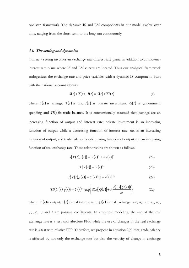
3.1. The setting and dynamics

Our new setting involves an exchange rate-interest rate plane, in addition to an income-

interest rate plane where IS and LM curves are located. Thus our analytical framework

endogenizes the exchange rate and price variables with a dynamic IS component. Start

with the national account identity:

tTBtGtItTtS (1)

where tS is savings, tT is tax, tI is private investment, tG is government

spending and tTB is trade balance. It is conventionally assumed that: savings are an

increasing function of output and interest rate; private investment is an increasing

function of output while a decreasing function of interest rate; tax is an increasing

function of output; and trade balance is a decreasing function of output and an increasing

function of real exchange rate. These relationships are shown as follows:

11 1,γa

trtYtrtYS (2a)

2αtYtYT (2b)

23 1,γa

trtYtrtYI

(2c)

dt

tQLndδtQLnβtYtqtYTB

αexp, 4 (2d)

where tY is output, tr is real interest rate, tQ is real exchange rate; 1α , 2α , 3α , 4α ,

1ζ , 2ζ , β and δ are positive coefficients. In empirical modeling, the use of the real

exchange rate is a test with absolute PPP, while the use of changes in the real exchange

rate is a test with relative PPP. Therefore, we propose in equation 2(d) that, trade balance

is affected by not only the exchange rate but also the velocity of change in exchange

6

rates. Different people may have different views on whether a currency is undervalued or

overvalued and the extent to which the currency is undervalued/ overvalued, and

adoption of different measures would lead to assigning different values to the real

exchange rate. Nevertheless, changes in real exchange rates would send out a signal as to

the currency’s depreciation or appreciation, thus having impact on trade balance. In a

recent survey by International Monetary Fund (IMF), it has been documented that

exchange rate changes were associated with growing net exports for the depreciating

countries, a development that is part of the natural adjustment process to differential

growth rates that flexible exchange rates promote. ‘Historical experience in advanced and

emerging market and developing economies suggests that exchange rate movements

typically have sizable effects on export and import volumes. A 10 percent real effective

depreciation in an economy’s currency is associated with a rise in real net exports of, on

average, 1.5 percent of GDP, with substantial cross-country variation around this

average’ (International Monetary Fund 2015). Auboin and Ruta (2011) have conducted a

comprehensive review of the literature and summarized that ‘A number of papers have

looked at the empirical relationship between exchange rate devaluation and export

surges. …, find that depreciation encourages exports for most countries’. They have

further remarked ‘The policy and academic debate shifted somewhat at this time, away

from the effects on trade of exchange volatility towards the effects of sustained exchange

rate depreciation or perceived exchange rate misalignments’, indicating the role of human

perception played in achieving or failing to achieve a consensus on right exchange rate

levels.

The real exchange rate in logarithms, by definition, is:

fptptetQLntq (3)

7

where te is nominal exchange rate, tp is price of goods and fp is foreign price of

goods, all in logarithms. Bringing equations (2a), (2b), (2c) and (2d) into equation (1)

yields:

tGdt

tQLndδtQLnβtrtY

γa

exp1 (4)

where 0α is an aggregate of 1α , 2α , 3α and 4α , and 0γ is an aggregate of 1γ and

2γ . The logarithmic form of equation (3) is derived as:

tgdt

tdqδtqβtrγtay (4’)

where 04321 ααααα and 021 γγγ . The LM component is

conventionally adopted, being derived from the liquidity of money equation:

λη

tr

tYtYtrL

tP

tM

1, (5)

where sdtMtMtM is demand for money that is equal to money supply in

equilibrium, and η and λ are positive coefficients. Taking the logarithmic transformation

leads to:

trλtyηtptm (5’)

All the variables in the above equation are in logarithms. Equation (4’) and equation (5’)

constitute a dynamic IS-LM system. All the variables can be endogenous in theory at this

stage, while certain variables can become exogenous or remain constant under various

circumstances, given the orientation of modeling or policy analysis.

The IS-LM system on the income-interest rate plane treats the real exchange rate,

alongside demand for money and government expenditure, as exogenous or as a policy

instrument for altering the level of interest rates and income. We extend and map the IS-

LM system to the exchange rate-interest rate plane, so the real exchange rate, as well as

the nominal exchange rate and price, becomes endogenous. We depart further from the

8

conventional static IS-LM analysis. Given an increase in money supply of dm , the

interest rate would be reduced by λ

dm in equation (5’), with no change in price and

income. Correspondingly in equation (4’), it is required that

dmλ

γ

dt

tdqδtqβ

,

which rectifies one of the major defects in the static IS-LM model. The following

remarks elucidate the issue.

In the static IS-LM model where δ = 0, tq is required to be reduced by dmβλ

γ,

given no change in income and government spending. This in turn indicates that te is

reduced by the same degree, given no immediate change in price. A reduction in tq or

te means appreciation of the domestic currency, which is implausible. We question this

judiciousness. A domestic interest rate that is lower than the world level of interest rates

would result in the domestic currency to appreciate, which takes time. For example and

assuming that the domestic interest rate remains unchanged at this lower level for one

year, it would take one year for the domestic currency to appreciate by λ

dm according to

interest rate parities. In our model with δ > 0, it is not required for tq to be reduced by

dmβλ

γ immediately to attain the new temporary equilibrium in the goods market,

tq could increase as well. The shift is realized by the velocity of exchange rate changes,

which makes the system dynamic meanwhile. Bringing equation (3) into equation (4)

leads to:

tgtyαpβdt

tdpδtpβtrγ

dt

tdeδteβ f (6)

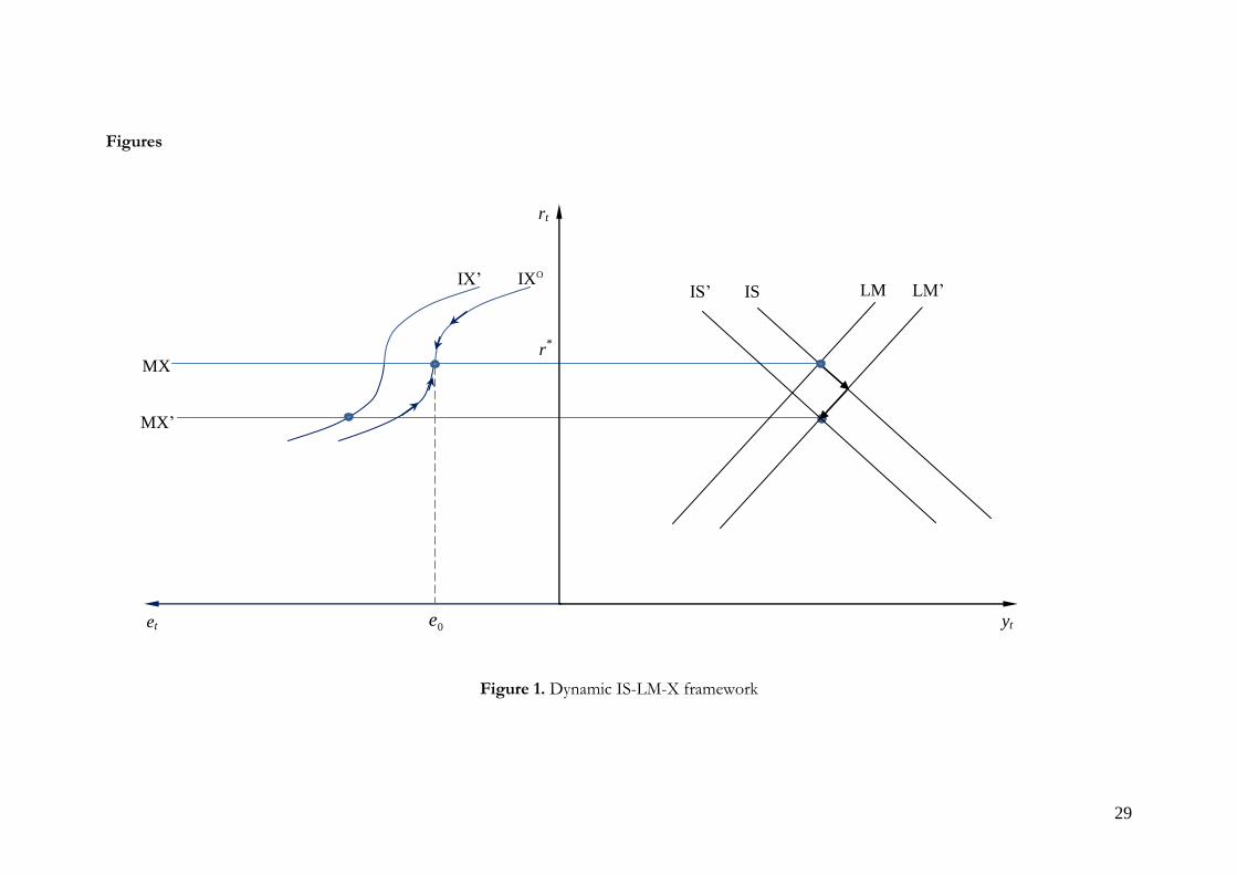
The dynamic equilibrium IS-LM-X model represented by equation (6) is illustrated

in Figure 1. The right side panel is the traditional IS-LM analysis on the income-interest

9

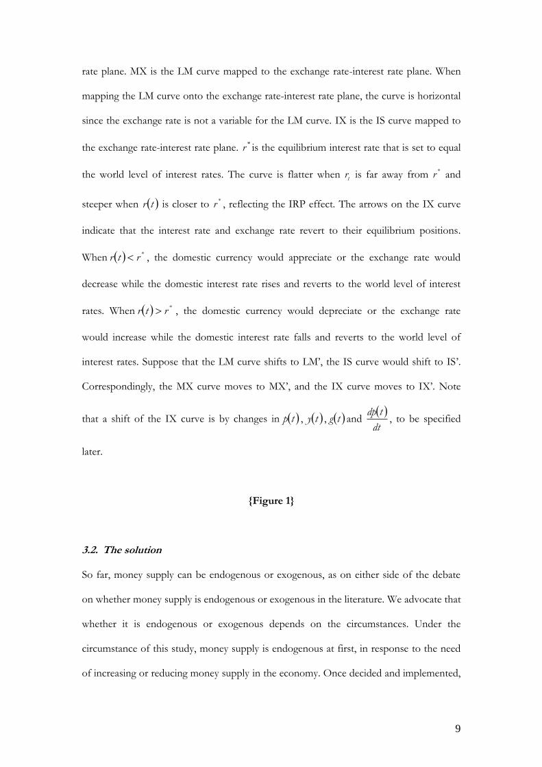
rate plane. MX is the LM curve mapped to the exchange rate-interest rate plane. When

mapping the LM curve onto the exchange rate-interest rate plane, the curve is horizontal

since the exchange rate is not a variable for the LM curve. IX is the IS curve mapped to

the exchange rate-interest rate plane. *r is the equilibrium interest rate that is set to equal

the world level of interest rates. The curve is flatter when tr is far away from *r and

steeper when tr is closer to *r , reflecting the IRP effect. The arrows on the IX curve

indicate that the interest rate and exchange rate revert to their equilibrium positions.

When *rtr , the domestic currency would appreciate or the exchange rate would

decrease while the domestic interest rate rises and reverts to the world level of interest

rates. When *rtr , the domestic currency would depreciate or the exchange rate

would increase while the domestic interest rate falls and reverts to the world level of

interest rates. Suppose that the LM curve shifts to LM’, the IS curve would shift to IS’.

Correspondingly, the MX curve moves to MX’, and the IX curve moves to IX’. Note

that a shift of the IX curve is by changes in tp , ty , tg and

dt

tdp, to be specified

later.

{Figure 1}

3.2. The solution

So far, money supply can be endogenous or exogenous, as on either side of the debate

on whether money supply is endogenous or exogenous in the literature. We advocate that

whether it is endogenous or exogenous depends on the circumstances. Under the

circumstance of this study, money supply is endogenous at first, in response to the need

of increasing or reducing money supply in the economy. Once decided and implemented,

10

it remains exogenous and constant until the next monetary policy change, which is the

assumption for the dynamics and solution of the model developed thereafter. Assume

that the system is in equilibrium at 0t , with mm 0 , pp 0 , yy 0 , rr 0 ,

ee 0 and gg 0 ; and the equilibrium interest rate is set to equal the world level of

interest rates *rr . Given an increase in money supply at time 0+, the money market

equilibriums before and after the increase in money supply are:

0000 rλyηpm (5’a)

0000 rλyηpdmm (5’b)

The domestic interest rate, corresponding to the monetary expansion, is reduced by:

λ

dmrr 00

(7)

according to equation (5’), since the price is fixed in the short-term and output is not

supposed to be affected, i.e., 00 pp , 0yty . The domestic interest rate

assumes a function form with which it rises gradually in reverting1 to the world level of

interest rates at speedφ :

tφeλ

dmrtr *

(8)

It stipulates that λ

dmrtr * at 0t as a consequence of the increase in money

supply signified by equation (7), then tr rises gradually at speed φ and *rtr when

t . Then the price of goods rises in the same way as follows:

dmeptp tφ 10 (9)

for the money market to clear continuously. It stipulates that 0ptp at 0t as the

price does not rise immediately; and dmptp 0 when t which

indicates dmptp 0 , i.e., the increase in goods price is equal to the increase in

money supply in the long-run when the effect of the increase in money supply on the

11

price is fully taken. Conforming to the Fisher effect, the price rises at the same speed φ

as the interest rate. The goods market equilibriums before and after the increase in

money supply are:

00000 gyαpβpβrγeβ f (6a)

00 gyαpβdt

tdpδtpβtrγ

dt

tdeδteβ f (6b)

with 0yty and 0gtg . Subtracting equation (6a) from equation (6b) yields:

dt

tdpδptpβrtrγeteβ

dt

tdeδ 00 * (10)

There is feedback from the exchange rate itself, and indirect feedback through the

interest rate and price loops, shown in the above equation. Given equation (8), equation

(9) and

dmeφdt

tdp tφ , the above can be re-arranged to:

dmeλ

γβδφdmβeβteβ

dmeδφdmeβdmeλ

γeβteβ

dt

tdeδ

tφ

tφtφtφ

0

10

(11)

which is a first-order linear non-autonomous constant parameter differential equation

and has a general solution of:

0,0

10

ttCeedm

φδ

βδλ

γφ

δ

β

dme

Cdtedmeλ

γβδφ

δdm

δ

βe

δ

βete

tδ

β

tφ

dtδ

β

tφdt

δ

β

(12)

C is solved by taking the boundary conditions into consideration:

12

dm

φδ

βδλ

γ

ee

dm

φδ

βδλ

γφ

δ

β

eeC

00

100

(13)

Conclusively, the exchange rate moves and evolves as follows:

0,0010

000

tteedm

φδ

βδλ

γφ

δ

β

eeedmee

edm

φδ

βδλ

γφ

δ

β

edm

φδ

βδλ

γ

eeedmete

tφt

δ

βt

δ

βt

δ

β

tφt

δ

βt

δ

β

(14)

It is apparent that tdmete ,0 . The features of the model and each of its

elements are discussed in the next section.

3.3. Rational and constrained expectations

The above analysis has implicitly incorporated the formation of expectations that is

constrained and rational. According to IRP, the expected changes in exchange rates equal

to the interest rate differentials:

**

***

πtπrtr

πrtπtritidt

tdeE

(15)

or:

dtπtπrtr

dtπrtπtrdtititdeE

**

***

(15’)

where ti is nominal interest rate, *i is world nominal interest rate, tπ is inflation rate,

*π is world inflation rate2. Equation (15) is IRP as well as international Fisher effect

13

(IFE). It is rational expectations, being constrained by IRP and IFE with both short-term

and long-run effects and implications. However, while equation (15) constrains a rational

expectations formation in the money market, the evolution paths of real and nominal

interest rates and inflation are further constrained and regulated by the relationships in

the goods markets in the dynamic IS-LM system. The trajectory portrayed by equation

(15) should be the same as the trajectory of equation (11) and its solution equation (14)

under rational and constrained expectations. The unstructured IRP and IFE of equation

(15) interact with and in the structured dynamic IS-LM system to offer a rational and

constrained solution.

4. The features of the model

We focus on the evolution path of the exchange rate after the shock in this study, and

leave 0e unsolved and subject it to actual figures. Findings in the empirical literature

imply that 0e is not predictable or can’t be modeled, as indicated in Section 2. The

second term on the right hand side of equation (14) increases gradually from 0 at 0t to

dm when t . The third term is the initial shock effect, which fades away eventually as

t . Given the initial effect is domestic currency depreciation to varied degrees, as

evident in the above reviewed studies, 000 ee . Therefore, the third term

decreases over time. The fourth term starts at 0 at 0t and approaches 0 when t .

It is concave or has a minimum value, which can be proved as follows. 0δλ

γφ

δ

β,

given that the elasticity or sensitivity parameters are smaller than unity. Then,

0

φδ

βδλ

γφ

δ

β

if φδ

β ; and 0

φδ

βδλ

γφ

δ

β

if φδ

β . So, it is required to prove that

14

tφt

δ

β

ee

is concave or has a minimum for φδ

β and tφ

tδ

β

ee

is convex or has a

maximum for φδ

β . In the case when φ

δ

β , t

δ

β

tφtφ

tδ

β

δ

βφ

etet

φδ

β

eeLim

.

Technical proofs are provided in Appendix A. Given the proofs, the fourth term

decreases first and then increases, featuring initial appreciation of the domestic currency

after the monetary shock.

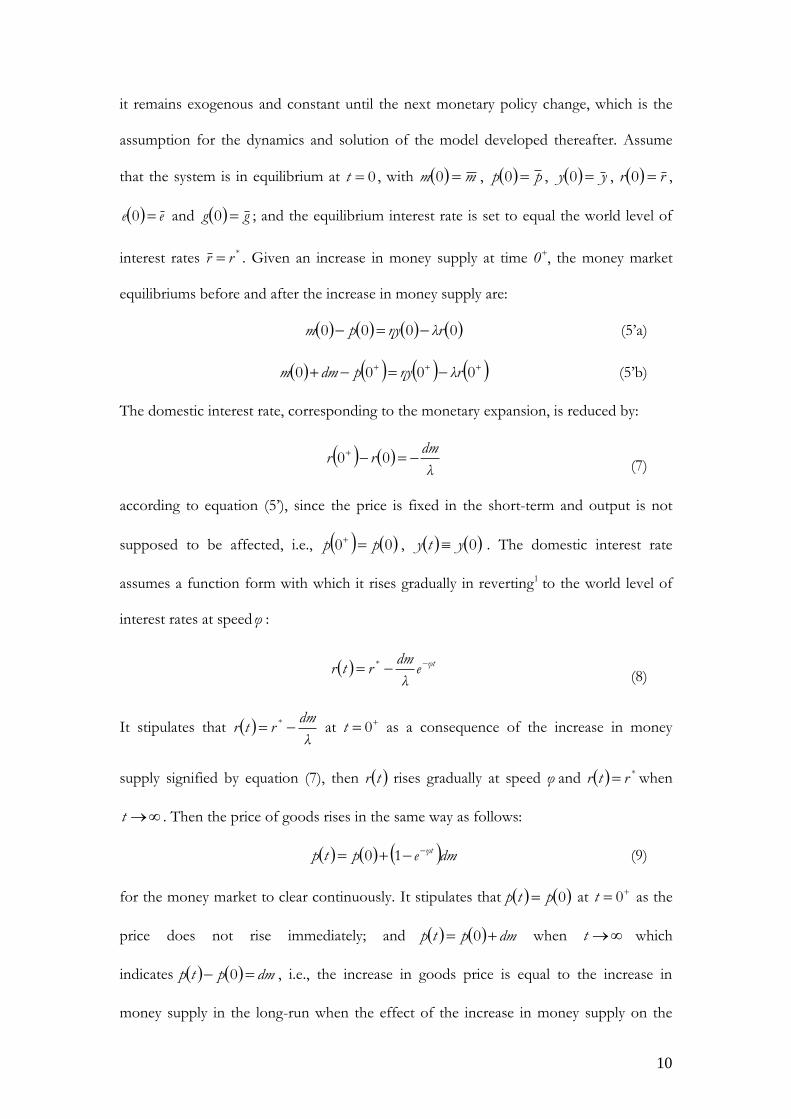
{Figure 2}

Finally, we inspect the overall pattern in exchange rate evolutions, combining the

features of individual elements. The domestic currency would appreciate initially after the

shock, and then depreciate towards its new long-run equilibrium rate. The exchange,

starting at 0e , decreases and reaches its minimum emin at tm , shown in Appendix B. That

is, the domestic currency would appreciate initially after the shock, and then depreciate

towards its new long-run equilibrium level dme 0 . These are exhibited in Figure 2 with

the patterns in each element of equation (14) and the overall pattern in exchange rate

adjustments and evolutions.

The above demonstrated pattern of exchange rate evolution is consistent with that

in a recent study of Wang (2013). Upon an increase in money supply, the interest rate

falls with IRP taking effect initially, with which the currency appreciates, and then the

sticky price rises gradually from the medium-term and over the long-run, in which the

currency depreciates. He has demonstrated three cases that initially reversely shoots, over

shoots and under shoots respectively. All of them make reverse movements after the

initial shock in the short-term, be the initial response overshooting, undershooting or

15

reverse shooting. Unlike Wang (2013) who assumes a short-term exchange rate target in

addition to a long-run equilibrium exchange rate, our model sets no short-term target at

all and no new long-run equilibrium exchange rate explicitly. It lets the open economy

evolves itself. The design of our model is also coherent with, but extends, the joint

dynamics of exchange rates and interest rates of Anderson et al. (2010) who apply the

affine class of term structure models to exchange rate movements as diffusion processes.

The evolution path of exchange rates in our model goes beyond the horizon when IRP

effects have diminished to a negligible extent.

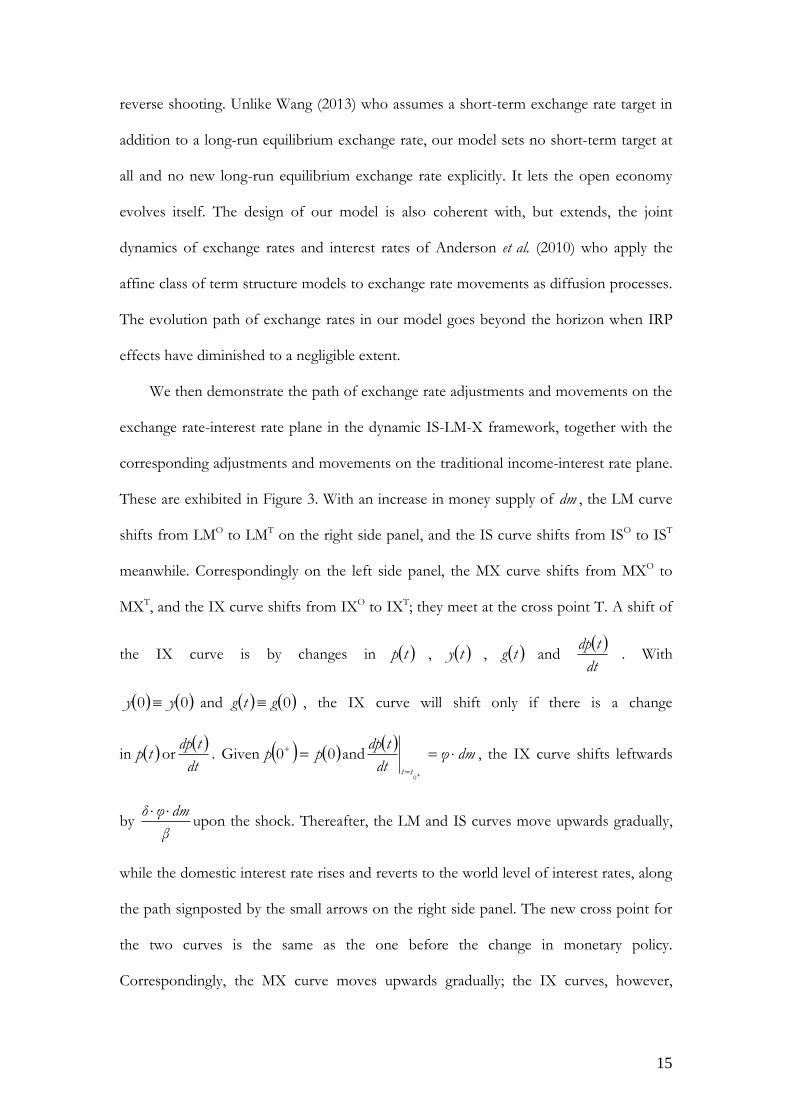
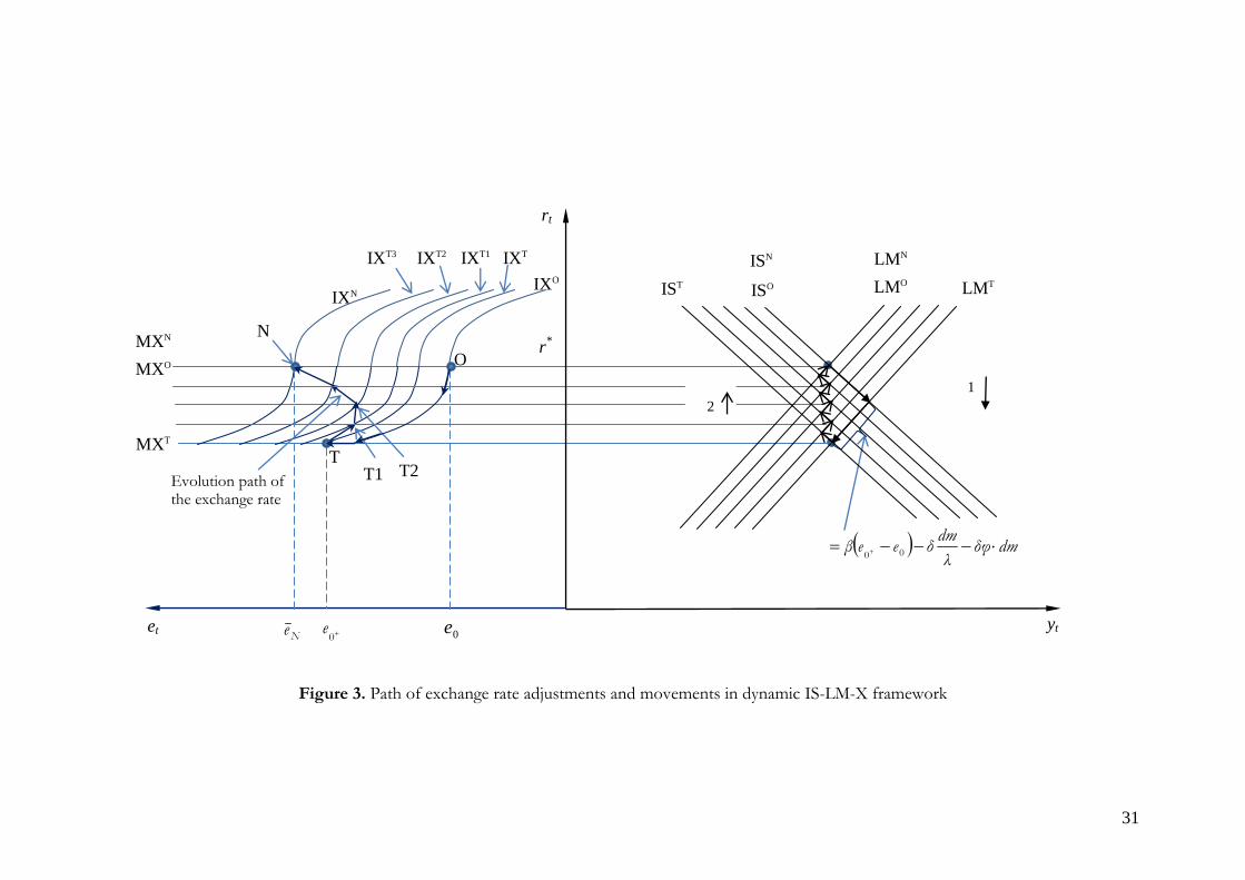
We then demonstrate the path of exchange rate adjustments and movements on the

exchange rate-interest rate plane in the dynamic IS-LM-X framework, together with the

corresponding adjustments and movements on the traditional income-interest rate plane.

These are exhibited in Figure 3. With an increase in money supply of dm , the LM curve

shifts from LMO to LMT on the right side panel, and the IS curve shifts from ISO to IST

meanwhile. Correspondingly on the left side panel, the MX curve shifts from MXO to

MXT, and the IX curve shifts from IXO to IXT; they meet at the cross point T. A shift of

the IX curve is by changes in tp , ty , tg and

dt

tdp. With

00 yy and 0gtg , the IX curve will shift only if there is a change

in tp or

dt

tdp. Given 00 pp and

dmφ

dt

tdp

tt

0

, the IX curve shifts leftwards

by β

dmφδ upon the shock. Thereafter, the LM and IS curves move upwards gradually,

while the domestic interest rate rises and reverts to the world level of interest rates, along

the path signposted by the small arrows on the right side panel. The new cross point for

the two curves is the same as the one before the change in monetary policy.

Correspondingly, the MX curve moves upwards gradually; the IX curves, however,

16

moves leftwards gradually until

0tdt

tdpand dmptp

t

0 . The total distance

the IX curve has traveled leftwards isdm when the system has settled down at the new

equilibrium point. The cross points of the corresponding MX and IX curves in their

shifts exhibit the path of exchange rate adjustments and movements. The MX and IX

curves meet at the cross point N when the system is in the new equilibrium. The shift of

the IS curve on the income-interest rate plane is by changes in

dt

tdqδtqβ , which can

also be expressed in the nominal exchange rate and prices:

dt

tdpδ

dt

tdeδpβtpβteβ

dt

tdqδtqβ f (16)

At 0

tt , fppe 00 = fppeee 0000 = 000 qee ,

λ

dm

dt

tde , and

dmφ

dt

tdp , so the shift of the IS curve upon the shock is:

dmδφλ

dmδeeβqβ 000 (17)

The downwards movement of the IS curve is enabled by the negative figures of

dmδφλ

dmδ , allowing the domestic currency to depreciate upon the shock, i.e.,

allowing the nominal exchange rate to increase. Otherwise, 0e has to be smaller than

0e .

{Figure 3}

While φ measures the swiftness of money market adjustments to attain the new

equilibrium,δ

βreflects the dynamics in goods market adjustments in moving to the

temporal equilibrium and then attaining the new equilibrium. If 0δ , goods market

17

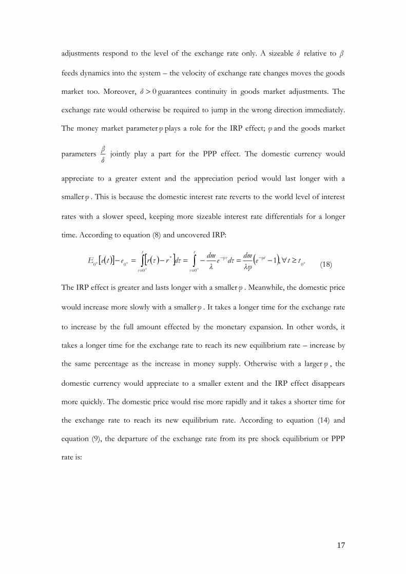
adjustments respond to the level of the exchange rate only. A sizeable δ relative to β

feeds dynamics into the system – the velocity of exchange rate changes moves the goods

market too. Moreover, 0δ guarantees continuity in goods market adjustments. The

exchange rate would otherwise be required to jump in the wrong direction immediately.

The money market parameterφ plays a role for the IRP effect; φ and the goods market

parameters δ

β jointly play a part for the PPP effect. The domestic currency would

appreciate to a greater extent and the appreciation period would last longer with a

smallerφ . This is because the domestic interest rate reverts to the world level of interest

rates with a slower speed, keeping more sizeable interest rate differentials for a longer

time. According to equation (8) and uncovered IRP:

0

00

*

00,1 tte

λφ

dmτde

λ

dmτdrτreteE tφ

t

τ

φτ

t

τ (18)

The IRP effect is greater and lasts longer with a smallerφ . Meanwhile, the domestic price

would increase more slowly with a smallerφ . It takes a longer time for the exchange rate

to increase by the full amount effected by the monetary expansion. In other words, it

takes a longer time for the exchange rate to reach its new equilibrium rate – increase by

the same percentage as the increase in money supply. Otherwise with a larger φ , the

domestic currency would appreciate to a smaller extent and the IRP effect disappears

more quickly. The domestic price would rise more rapidly and it takes a shorter time for

the exchange rate to reach its new equilibrium rate. According to equation (14) and

equation (9), the departure of the exchange rate from its pre shock equilibrium or PPP

rate is:

18

0,000

0000

10

0010

tteedm

φδ

βδλ

γ

eeeq

eedm

φδ

βδλ

γ

eeeppe

pdmep

eedm

φδ

βδλ

γφ

δ

β

eeedmee

ptptetq

tφt

δ

βt

δ

β

tφt

δ

βt

δ

β

f

ftφ

tφt

δ

βt

δ

βt

δ

β

f

(19)

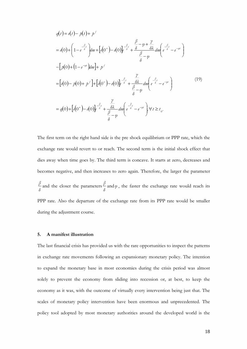
The first term on the right hand side is the pre shock equilibrium or PPP rate, which the

exchange rate would revert to or reach. The second term is the initial shock effect that

dies away when time goes by. The third term is concave. It starts at zero, decreases and

becomes negative, and then increases to zero again. Therefore, the larger the parameter

δ

βand the closer the parameters

δ

βandφ , the faster the exchange rate would reach its

PPP rate. Also the departure of the exchange rate from its PPP rate would be smaller

during the adjustment course.

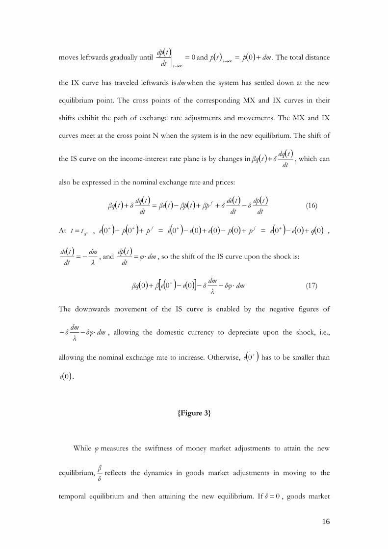
5. A manifest illustration

The last financial crisis has provided us with the rare opportunities to inspect the patterns

in exchange rate movements following an expansionary monetary policy. The intention

to expand the monetary base in most economies during the crisis period was almost

solely to prevent the economy from sliding into recession or, at best, to keep the

economy as it was, with the outcome of virtually every intervention being just that. The

scales of monetary policy intervention have been enormous and unprecedented. The

policy tool adopted by most monetary authorities around the developed world is the

19

most direct amongst the three major policy tools – large scale open market purchases of

bonds and gilts or quantitative easing (QE). Unlike “conventional” monetary expansions

where changes in a few other economic variables may influence exchange rates as much

as money supply does, the effect of QE on exchange rates and exchange rate movements

greatly dwarfs that of any other economic variables. For this reason, QE effectively

isolates the impact of other economic variables on exchange rate movements from that

of monetary expansions, offering an immaculate environment in which the effect of

monetary expansions on exchange rate adjustment and movement is studied.

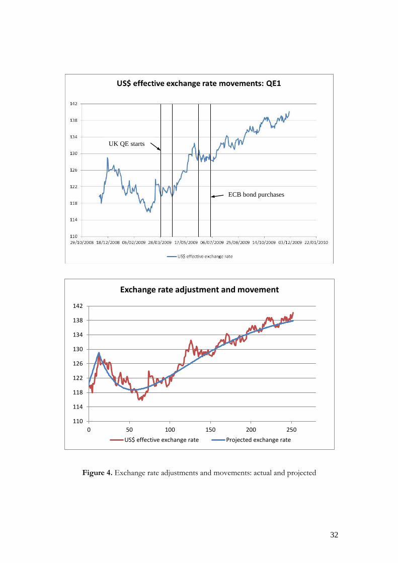
The first round of QE in the US, QE1, is used for case analysis. QE1 started in

December 2008 when the Federal Reserve announced it would purchase up to $100

billion in agency debt and up to $500 billion in agency mortgage-backed securities on

November 25, 2008. Although the purchases spread over a period, that period was fairly

short. The announcement effect would be also considerable, which Gagnon et al. (2010)

scrutinize for QE1 in detail. The exchange rate used in the study is the US dollar

effective exchange rate provided by the US Federal Reserve. The effective exchange rate

is re-arranged so that an increase in it corresponds to the depreciation of the US dollar

vis-à-vis the currencies of its trading partners, the same way as directly quoted bilateral

exchange rates. Figure 4 exhibits US dollar effective exchange rate movements since the

start of QE1 in a one-year frame, by which time the rest of the developed economies had

also begun implementing their own QE programs and their asset purchases became

sizeable. For example, the MPC of the UK announced a £75b asset purchase plan over a

three-month period in March 2009; by the November MPC meeting asset purchases

were extended to £200b (cf. Joyce et al. 2011 for the design and operation of QE in the

UK). During this period, the ECB also adopted some kind of QE, albeit on a much

smaller scale, including a €60b corporate bond purchase program made known in May

2009. Observing Figure 4, US dollar effective exchange rate movements in QE1 fit the

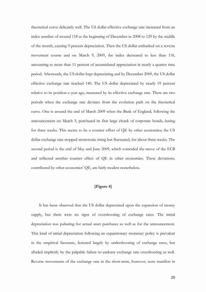
20

theoretical curve delicately well. The US dollar effective exchange rate increased from an

index number of around 118 at the beginning of December in 2008 to 129 by the middle

of the month, causing 9 percent depreciation. Then the US dollar embarked on a reverse

movement course and on March 9, 2009, the index decreased to less than 116,

amounting to more than 11 percent of accumulated appreciation in nearly a quarter time

period. Afterwards, the US dollar kept depreciating and by December 2009, the US dollar

effective exchange rate reached 140. The US dollar depreciated by nearly 19 percent

relative to its position a year ago, measured by its effective exchange rate. There are two

periods when the exchange rate deviates from the evolution path on the theoretical

curve. One is around the end of March 2009 when the Bank of England, following the

announcement on March 5, purchased its first large chunk of corporate bonds, lasting

for three weeks. This seems to be a counter effect of QE by other economies; the US

dollar exchange rate stopped monotonic rising but fluctuated, for about three weeks. The

second period is the end of May and June 2009, which coincided the move of the ECB

and reflected another counter effect of QE in other economies. These deviations,

contributed by other economies’ QE, are fairly modest nonetheless.

{Figure 4}

It has been observed that the US dollar depreciated upon the expansion of money

supply, but there were no signs of overshooting of exchange rates. The initial

depreciation was pulsating for actual asset purchases as well as for the announcement.

This kind of initial depreciation following an expansionary monetary policy is prevalent

in the empirical literature, featured largely by undershooting of exchange rates, but

alluded implicitly by the palpable failure to endorse exchange rate overshooting as well.

Reverse movements of the exchange rate in the short-term, however, were manifest in

21

QE. The US dollar depreciated inevitably afterwards in the long-run and the exchange

rate moved inevitably in a depreciating manner. The displayed pattern in US dollar

effective exchange rate adjustments and movements mirror the theoretical analysis of this

paper remarkably agreeably.

6. Summary

A model of exchange rate adjustments in a dynamic IS-LM-X analytical framework has

been proposed in this paper, to analyze the adjustment and evolution path of the

exchange rate following a change in money supply. The proposed model firstly makes the

IS-LM model dynamic, and then endogenizes the exchange rate and price variables. It

extends the dynamic IS and LM components into the external sector in an open

economy that evolves continuously. Effects of IRP and PPP can be and are scrutinized

with this analytical framework as time goes by.

It can be observed that, following an expansionary monetary policy, the domestic

currency appreciates initially after the shock, prior to gradual depreciation towards its

new long-run equilibrium level that is the pre monetary expansion equilibrium rate plus

the percentage increase in money supply. This pattern in exchange rate adjustments and

movements is resulted from the joint and sequential effects of IRP and PPP. This pattern

in the evolution path of exchange rate adjustments and movements has manifested by

the recent example of the US QE in one of the most rattling epochs of the last financial

crisis. The actual exchange rate movements fit the theoretical curve delicately well.

References

Anderson, B., Hammond, P.J. and Ramezani, C.A. (2010), Affine models of the joint

dynamics of exchange rates and interest rates, Journal of Financial and Quantitative

Analysis 45, 1341-1365.

22

Auboin, M. and Ruta, M. (2011), The relationship between exchange rates and

international trade: a review of economic literature, Staff Working Paper ERSD-2011-

17, Economic Research and Statistics Division, World Trade Organization, Genève,

Switzerland.

Bjørnland, H.C. (2009), Monetary policy and exchange rate overshooting: Dornbusch

was right after all, Journal of International Economics 79, 64-77.

Branson, W.H., “Asset markets and relative prices in exchange rate determination,” IIES

Seminar Paper No. 66, 1976.

Cavaglia, S. (1991), Permanent and transitory components in the time series of real

exchange rates, Journal of International Financial Markets, Institutions and Money 1, 1-44.

Dornbusch, R. (1976), “Expectations and exchange rate dynamics,” Journal of Political

Economy 84, 1161-1176.

Fleming, J.M. (1962), Domestic financial policies under fixed and floating exchange rates,

IMF Staff Papers 9, 369–79.

Frankel, J.A. (1979), “On the mark: a theory of floating exchange rates based on real

interest differentials,” American Economic Review 69, 610-622.

Frenkel, J.A. (1976), “A monetary approach to the exchange rate: doctrinal aspects and

empirical evidence,” Scandinavian Journal of Economics 78, 200-224.

Gagnon, J., Raskin, M., Remache, J. and Sack, B. (2010), Large-scale asset purchases by

the Federal Reserve: did they work? Quantitative Easing Conference, the Federal Reserve

Bank of St. Louis.

Heinlein, R. and Krolzig, H.M. (2012), Effects of monetary policy on the US dollar/UK

pound exchange rate – is there a “delayed overshooting puzzle”? Review of International

Economics 20, 443-467.

Hwang, J.K. (2003), Dynamic forecasting of sticky-price monetary exchange rate model,

Atlantic Economic Journal 31, 103-114.

23

International Monetary Fund (2015), World Economic Outlook: Adjusting to Lower Commodity

Prices, Washington, D.C..

Joyce, M., Tong, M. and Woods, R. (2011), The United Kingdom’s quantitative easing

policy: design, operation and impact, Quarterly Bulletin Q3, Bank of England.

Levin, J.H. (1994), On sluggish output adjustment and exchange rate dynamics, Journal of

International Money and Finance 13, 447-458.

Meese, R. and K. Rogoff (1988), “Was it real? The exchange rate-interest differential

relation over the modern floating-rate period,” Journal of Finance 43, 933-948.

Mundell, R.A. (1963), Capital mobility and stabilization policy under fixed and flexible

exchange rates, Canadian Journal of Economics and Political Science 29, 475-485.

Mussa, M. (1982), A model of exchange rate dynamics, Journal of Political Economy 90, 74-

104.

Verschoor, W.F.C. and Wolff, C.C.P. (2001), Exchange risk premia, expectations

formation and “news” in the Mexican peso/US dollar forward exchange rate market,

International Review of Financial Analysis 10, 157-174.

Wang, P.J. (2013), Reverse shooting of exchange rates, Economic Modelling 33, 71-76.

Zita, S. and Gupta, R. (2008), Modeling and forecasting the Medical-Rand exchange rate,

ICFAI Journal of Monetary Economics 6, 63-90.

Endnotes

1 In relativity, other economies’ interest rates converge/revert to the domestic interest rate for a large open economy, while the latter reverts to its own long-run equilibrium rate. 2 In the literature, the real interest rate is assumed to be equalized across countries in some studies, in particular in the derivation of IFE in textbooks; some others take the stance that real interest rates vary across countries and over time. We assume the latter in this study.

24

Appendix A

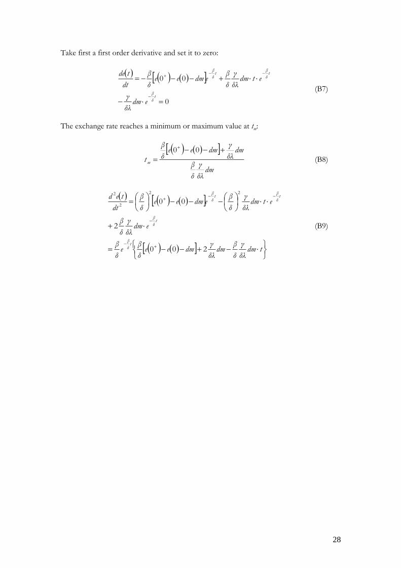
Take a first order derivative and set it to zero:

0

tδ

β

tφ

tφt

δ

β

eδ

βeφ

dt

eed

(A1)

It reaches a minimum or maximum at time tm:

φδ

β

δφ

βLn

t m

(A2)

Note 0

δφ

βLn when φ

δ

β and 0

δφ

βLn when φ

δ

β , so the sign of the

numerate and the sign of the denominator are always the same, tm being guaranteed to be

positive, definite. So tm ℝ++ and is always viable. At t = tm, the second order derivative

is:

δφ

βLnφ

δ

β

δφ

βLn

δ

β

δφ

βLnφ

δ

β

δφ

βLn

δ

β

φδ

β

δφ

βLn

φδ

β

φδ

β

δφ

βLn

δ

β

φδ

β

δφ

βLn

φ

φδ

β

δφ

βLn

δ

β

tt

tφt

δ

β

eδφ

βφeeφ

δ

βe

eφδ

βe

eφeδ

β

dt

eed

m

2

22

2

2

2

2

2

2

2

(A3)

Therefore, whether the second order derivative is positive or negative is decided by the

sign of

δφ

βLn

eδφ

β2

. Since:

25

φδ

β

φδ

β

δφ

βLn

δφ

βLn

δφ

βLn2 (A4)

Therefore:

φδ

β

φδ

β

tt

tφt

δ

β

m

dt

eed

0

0

2

2

(A5)

That is, tφt

δ

β

ee

is concave for φδ

β and tφ

tδ

β

ee

is convex for φδ

β .

So the fourth term of equation (14)

tφ

tδ

β

eedm

φδ

βδλ

γφ

δ

β

is always concave, given

that 0

φδ

βδλ

γφ

δ

β

if φδ

β and 0

φδ

βδλ

γφ

δ

β

if φδ

β .

Whenδ

βφ , the above analysis does not hold, where

0

0

φδ

β

ee tφt

δ

β

. For δ

βφ ,

φδ

β

ee tφt

δ

β

takes the form of:

tδ

β

tφtφ

δ

βφ

tφt

δ

β

δ

βφ

etette

Lim

φδ

β

eeLim

1

(A6)

Take the first order derivative and set it to zero:

01

tφedt

ted tφtφ

It reaches a minimum or maximum at time tm:

26

φ

t m

1

At t = tm, the second order derivative is:

0

12 1

1

2

2

eφφ

φeφdt

ted φφ

tt

tφ

m

Therefore, fourth term of equation (14)

tφ

tδ

β

eedm

φδ

βδλ

γφ

δ

β

is always concave

whenδ

βφ .

Appendix B

Express equation (14) in a condensed way:

0,1000 ttedmedmeedmete tφt

δ

β

(B1)

where

φδ

β

φδ

β

φδ

βδλ

γφ

δ

β

0

0

. Take first a first order derivative and set it to zero:

0100

tδ

β

tφ edmeeδ

βedmφ

dt

tde (B2)

The exchange rate reaches a minimum or maximum value at tm, which can be solved by:

φδ

β

dmβ

δφ

dmeeLn

t m

100

(B3)

which additionally requires:

0,0100 dmee (B4a)

27

0,0100 dmee (B4b)

otherwise the trajectory would be monotonous without a turning point. It reduces to

equation (A2) when dmee 00 . At t = tm, the second order derivative of the

exchange rate with respect to t is:

β

δφφ

δ

β

dmβ

δφ

dmeeLn

δ

β

φδ

β

dmβ

δφ

dmeeLn

φ

φδ

β

dmβ

δφ

dmeeLn

δ

β

tt

edmβ

φδdmee

δ

βe

edmφ

edmeeδ

β

dt

ted

m

22

100

100

2

100

2

2

2

100

100

(B4)

The sign of the second order derivative is the same as the sign of

β

δφ

edmβ

φδdmee

2

100 . Therefore, the exchange rate reaches a

minimum value at tm if:

dmedmβ

φδee β

δφ

100

2

(B5)

in conjunction with equation (B4a) and equation (B4b).

Whenδ

βφ , the above analysis does not hold, where

0

0

φδ

β

ee tφt

δ

β

. Take in the result in

equation (A6), equation (14) becomes:

0,000 tttedmδλ

γedmeedmete

tδ

βt

δ

β

(B6)

28

Take first a first order derivative and set it to zero:

0

00

tδ

β

tδ

βt

δ

β

edmδλ

γ

etdmδλ

γ

δ

βedmee

δ

β

dt

tde

(B7)

The exchange rate reaches a minimum or maximum value at tm:

dmδλ

γ

δ

β

dmδλ

γdmee

δ

β

t m

00

(B8)

tdmδλ

γ

δ

βdm

δλ

γdmee

δ

βe

δ

β

edmδλ

γ

δ

β

etdmδλ

γ

δ

βedmee

δ

β

dt

ted

tδ

β

tδ

β

tδ

βt

δ

β

200

2

00

22

2

2

(B9)

29

Figures

Figure 1. Dynamic IS-LM-X framework

IS LM

yt

rt

r*

IXO

0e et

IX’

MX

MX’

IS’ LM’

30

(a) Patterns in three terms

(b) Patterns in exchange rate adjustment and movement in logarithm

(c) Exchange rates

Figure 2. Exchange rate adjustment and movement

0.000

0.020

0.040

0.060

0.080

0.100

0 50 100 150 200 250 300

0.000

0.003

0.006

0.009

0 50 100 150 200 250 300

-0.120

-0.090

-0.060

-0.030

0.000

0 50 100 150 200 250 300

0.175

0.225

0.275

0.325

0 50 100 150 200 250 300

exchange rate in logarithm

1.15

1.20

1.25

1.30

1.35

1.40

0 50 100 150 200 250 300

Exchange rate asjustment and movement

exchange rate

31

Figure 3. Path of exchange rate adjustments and movements in dynamic IS-LM-X framework

O

MXT

IXO

Evolution path of the exchange rate

T

r*

N

T2

Ne 0e 0e et

IXT1

IXN

MXO

MXN

T1

IXT3 IXT IXT2

dmδφ

λ

dmδeeβ 00

yt

LMO IST LMT

rt

2

1

ISN

ISO

LMN

32

Figure 4. Exchange rate adjustments and movements: actual and projected

UK QE starts

ECB bond purchases

110

114

118

122

126

130

134

138

142

0 50 100 150 200 250

Exchange rate adjustment and movement

US$ effective exchange rate Projected exchange rate