Embed Size (px)
Citation preview

Review of Economic Studies (2004)71, 581–611 0034-6527/04/00250581$02.00c© 2004 The Review of Economic Studies Limited
A Dynamic Analysis of the Marketfor Wide-Bodied Commercial
AircraftC. LANIER BENKARD
Graduate School of Business, Stanford University
First version received May2000; final version accepted March2003(Eds.)
This paper uses an empirical dynamic oligopoly model of the commercial aircraft industry to analyseindustry pricing, industry performance, and optimal industry policy. A novel feature of the model withrespect to the previous literature is that entry, exit, prices, and quantities are endogenously determined inMarkov perfect equilibrium (MPE). We find that many unusual aspects of the aircraft data, such as highconcentration and persistent pricing below static marginal cost, are explained by this model. We also findthat the unconstrained MPE is quite efficient from a social perspective, providing only 10% less welfareon average than a social planner would obtain. Finally, we provide simulation evidence that an anti-trustpolicy in the form of a concentration restriction would be welfare reducing.
1. INTRODUCTION
Due to steep learning curves and high entry costs, the commercial aircraft industry is an industryin which many conventional wisdoms of static economic theories do not apply. For example, asfirms work down their learning curves it is common to observe prices that are well below staticmarginal cost, a result that is inconsistent with static profit maximization. The aircraft industryhas also been a frequent target of industrial policy, most notably in Europe, and is subject toseveral special trade agreements, including the 1979 GATT agreement and the 1992 bilateralagreement between the U.S. and Europe. These issues have been addressed in part in the recenttheory literature (Spence(1981), Fudenburg and Tirole(1983), Dasgupta and Stiglitz(1988),Cabral and Riordan(1994) and others) as well as in the recent international trade literature(Baldwin and Krugman(1988), Klepper(1990), Tyson(1992)). The approach of this paper isto use a fully specified empirical dynamic model. Our hope is to gain a better understanding ofstrategic interaction in the industry, as well as to develop a framework in which to better evaluatetrade and anti-trust policies.
The past theoretical literature on learning by doing, which we use as guidance, hasfocused on two main areas. First, the literature has found that learning curves have importantstrategic implications. Pathbreaking papers bySpence(1981) andFudenburg and Tirole(1983)showed that learning curves can lead to a dynamic incentive to set the price below the level ofstatic marginal cost, especially upon the introduction of a new product.Dasgupta and Stiglitz(1988) showed that industries in which learning curves are steep may tend to become highlyconcentrated over time. The paper’s first goal is to test these theoretical models on industry data.We do this by estimating the primitives of a dynamic oligopoly model and then comparing theequilibrium predictions of the model with the observed data.
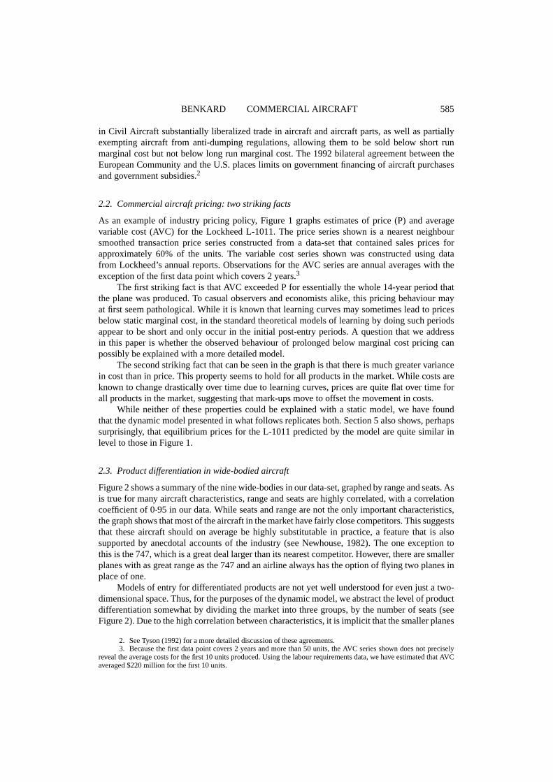
Additionally, we address the following striking empirical fact: data obtained for theLockheed L-1011 shows that price was below static marginal cost for essentially its entire14-year production run (seeFigure 1), for a total variable loss of approximately $2·5 billion
581

582 REVIEW OF ECONOMIC STUDIES
0 50 100 150 200 250
Mill
ion
Con
stan
t 199
4 D
olla
rs
Unit Number (Ordered by Delivery Date)
Estimated AVC
Nearest Neighbour (10 units) Smoothed Prices
40
50
60
70
80
90
100
110
120
FIGURE 1
Lockheed L-1011: price vs. AVC 1972–1985
current dollars.1 While this is the only aircraft model for which detailed cost data is available,data on profits for other firms suggests that many other aircraft have also been sold at a variableprofit loss. We investigate whether a dynamic oligopoly model with learning parameters thatare estimated from aircraft production data can explain this pricing behaviour, or whether, assuggested by some (e.g.Reinhardt, 1973), a rational firm should have set a higher price or exited.
The second area that the past theoretical literature has focused on is optimal policy.Dasgupta and Stiglitz(1988) showed that learning curves may lead to a specialized policyenvironment in which standard policy prescriptions may perform poorly. They showed that thereare situations in which an unrestrained monopolist may be socially preferable to any market withmore than one firm, which suggests that a blind application of existing anti-trust policies may notbe desirable in the commercial aircraft industry. They also showed that when learning is strongit may increase a country’s welfare to protect an infant industry.
While the theory literature has been very insightful and has vastly increased our under-standing of industries like this one, there are two weaknesses of the theoretical approach. Thefirst is that the theory models tend to be quite stylized, not reflecting any industry particularlywell. The second is that many of their predictions are ambiguous in practice: policy prescriptionstypically depend on the values of important model parameters such as learning rates and demandconditions. Both of these shortcomings point to the need for empirical work to provide a moredefinitive analysis. Thus, the second goal of this paper is to use our empirical model to investigateoptimal policy.
1. Source: author’s calculations based on Lockheed’s annual reports. This figure does not include developmentcosts of another $2·5 billion.

BENKARD COMMERCIAL AIRCRAFT 583
While even the simplest models of dynamic oligopoly can be quite complex, an empiricalanalysis of our questions of interest would not be possible without such a model. Because firmsmust introduce new aircraft models at prices below the level of static marginal cost while theywork down their learning curves, a static model would have difficulty justifying productionin many cases, let alone explaining why rational firms would pay entry costs in the billionsof dollars. Furthermore, understanding the initial post-entry period, in which large amounts ofsurplus are transferred from producers to consumers, is important to understanding the industry’soverall performance. Therefore, static models are not likely to provide a very useful analysis.We also show that the observed mark-ups are not consistent with single-agent optimization, butare consistent with equilibrium behaviour in oligopoly, so it would not be possible to simplifythe analysis by using a single-agent model. Finally, because dynamic profit incentives are ofprimary importance in the industry, a complete analysis of a policy change requires analysis ofthe equilibrium response of firms to the policy, which is only possible in an equilibrium model.
In developing the oligopoly model, we build on recent theoretical advances in modellingdynamic oligopoly byPakes and McGuire(1994, 2001) andEricson and Pakes(1995). Due tothe curse of dimensionality inherent to dynamic programming models, it would not normally befeasible to apply these discrete time, discrete state space, dynamic game models to a real worldindustry. However, the fact that the aircraft industry is a small oligopoly, with only a handful offirms and products, makes the approach computationally feasible.
This paper also makes several methodological contributions. The paper is among the firstempirical applications of a fully specified dynamic oligopoly model (cf.Gowrisankaran andTown, 1997). Our model is also a significant extension to the literature on computable discretetime dynamic games (e.g. Ericson and Pakes, 1995), as it is the first model of this type toincorporate dynamics in the product market equilibrium. In the previous literature (includingBerry and Pakes(1993), Pakes and McGuire(1994, 2001), Gowrisankaran(1999)), the productmarket was modelled as static price or quantity setting, with dynamics coming through firms’investment decisions. We feel that the extension of dynamics to the product market is potentiallyquite important for the I.O. literature because it covers several important cases in addition tolearning by doing, including durable goods, network effects, switching costs and others. NotethatFershtman and Pakes(2000) also allow for current prices to influence future states througha state variable that reflects past cooperation in a collusive scheme.
Our empirical strategy involves three steps. First, we write down a dynamic model that wefeel represents the industry well, maintaining the key features of the industry such as learningcurves, product differentiation, large entry costs and closed loop strategic interaction, whileabstracting away several less important features such as multi-unit demand. Second, we estimatethe primitives of the model. The model has both a supply and a demand system, which weestimate separately, in a manner that is consistent with the underlying dynamic model. Wesimultaneously estimate the stochastic processes determining the transition processes for thestate variables. Third, we numerically compute the equilibrium of the model, test the modelpredictions against the data, and evaluate several counterfactual policies.
There are several advantages to this three-step approach. Because equilibrium is notenforced in the estimation procedures, consistency of the parameter estimates does not dependon the equilibrium assumptions and is therefore robust to a wide set of possible assumptions.In addition, there is no need to solve the dynamic programming problem during estimation,which greatly reduces the computational burden of the estimation procedures. Finally, since theequilibrium behaviour of firms is not used in estimation, the equilibrium predictions of the modelcan be used as a test of the theoretical model. If the equilibrium model fits the data well, we takethat as evidence in support of the model. The main disadvantage of our approach is that, if theequilibrium assumptions are true, then greater efficiency could be obtained in the estimates by

584 REVIEW OF ECONOMIC STUDIES
enforcing equilibrium during estimation. Another disadvantage of this approach is that it doesnot easily provide a formal test of alternative models.
We find that, despite some simplifications, the dynamic model predicts many aspects ofequilibrium behaviour well, particularly those that have been the focus of the past theoreticalliterature. It improves vastly on previous attempts at modelling aircraft industry pricing (cf.Baldwin and Krugman(1988), Klepper(1990)). For example, even though observed mark-upsvary over a wide range, the model predicts both price levels and price movements that are similarto those observed, including many instances of below static marginal cost pricing. The modeltends to predict equilibrium prices and mark-ups that are slightly higher than those observed, butwe do not feel that this tendency is a shortcoming of the theoretical model. Rather, it is largelyattributable to an arbitrary dimensional restriction placed on the model for computational reasons.The model also represents many aspects of the industry dynamics well, generating entry, exit,concentration ratios, plane value and plane type distributions that are similar to those observed.
We also find that the model approximately replicates Lockheed’s pricing and exit strategiesfor the L-1011, suggesting that Lockheed’s behaviour was in fact consistent with profitmaximization. The results of the model suggest that Lockheed always had reason to expect areasonable chance of future success that, coupled with the incentive to move down its learningcurve, led to an incentive to continually price below static marginal cost, but not to exit.
The model is also well suited to a detailed analysis of industry performance. InSection7we consider three alternative market structures: single-product firms, a multi-product monopolistand a multi-product social planner (SP). The results from this comparison suggest that the single-product firm Markov perfect equilibrium (MPE) is quite efficient from a social perspective,providing only 10% less total welfare on average than the SP could obtain. However, relativeto the SP, the MPE shifts a substantial portion of total surplus from consumers to producers.We also find that an unconstrained multi-product monopolist with no threat of entry would leadto large inefficiencies from a social perspective. We go on to consider an anti-trust policy thatplaces a per se restriction on the highest market share any single firm may attain. This policy isequivalent to the type of policy considered inDasgupta and Stiglitz(1988). We find that such apolicy would be welfare reducing with very high probability, particularly hurting consumers.
2. THE COMMERCIAL AIRCRAFT INDUSTRY
2.1. Industry background
The commercial jet aircraft industry has existed since 1956, with the first wide-body introducedin 1969. In the empirical analysis, we focus on the market for wide-bodied commercial jetssince that market contains a more computationally tractable number of products than the entirecommercial aircraft market. Sales of wide-bodies have grown steadily since then so that in1997 they accounted for approximately 60% of total industry revenue (30% of units). Totalcommercial aircraft industry revenue for 1997 was approximately $60 billion, of which $40billion is attributable to U.S. producers. Commercial aircraft is also among the U.S.’s largestnet exports, with trade surpluses averaging about $25 billion annually over the early 1990s. Thecommercial aircraft industry, and aerospace more generally, has seen much merger activity inrecent years that has led to increased concentration. Currently, only two major producers remainfor commercial jets of more than 100 seats.
Many countries regard the commercial aircraft industry as a “strategic” industry. Assuch it has frequently been the target of industrial policy, most notably in Europe, wheregovernment supported efforts at developing a viable industry suffered many failures beforefinally experiencing success with the Airbus consortium. The 1979 GATT Agreement on Trade
BENKARD COMMERCIAL AIRCRAFT 585
in Civil Aircraft substantially liberalized trade in aircraft and aircraft parts, as well as partiallyexempting aircraft from anti-dumping regulations, allowing them to be sold below short runmarginal cost but not below long run marginal cost. The 1992 bilateral agreement between theEuropean Community and the U.S. places limits on government financing of aircraft purchasesand government subsidies.2
2.2. Commercial aircraft pricing: two striking facts
As an example of industry pricing policy,Figure1 graphs estimates of price (P) and averagevariable cost (AVC) for the Lockheed L-1011. The price series shown is a nearest neighboursmoothed transaction price series constructed from a data-set that contained sales prices forapproximately 60% of the units. The variable cost series shown was constructed using datafrom Lockheed’s annual reports. Observations for the AVC series are annual averages with theexception of the first data point which covers 2 years.3
The first striking fact is that AVC exceeded P for essentially the whole 14-year period thatthe plane was produced. To casual observers and economists alike, this pricing behaviour mayat first seem pathological. While it is known that learning curves may sometimes lead to pricesbelow static marginal cost, in the standard theoretical models of learning by doing such periodsappear to be short and only occur in the initial post-entry periods. A question that we addressin this paper is whether the observed behaviour of prolonged below marginal cost pricing canpossibly be explained with a more detailed model.
The second striking fact that can be seen in the graph is that there is much greater variancein cost than in price. This property seems to hold for all products in the market. While costs areknown to change drastically over time due to learning curves, prices are quite flat over time forall products in the market, suggesting that mark-ups move to offset the movement in costs.
While neither of these properties could be explained with a static model, we have foundthat the dynamic model presented in what follows replicates both.Section5 also shows, perhapssurprisingly, that equilibrium prices for the L-1011 predicted by the model are quite similar inlevel to those inFigure1.
2.3. Product differentiation in wide-bodied aircraft
Figure2 shows a summary of the nine wide-bodies in our data-set, graphed by range and seats. Asis true for many aircraft characteristics, range and seats are highly correlated, with a correlationcoefficient of 0·95 in our data. While seats and range are not the only important characteristics,the graph shows that most of the aircraft in the market have fairly close competitors. This suggeststhat these aircraft should on average be highly substitutable in practice, a feature that is alsosupported by anecdotal accounts of the industry (seeNewhouse, 1982). The one exception tothis is the 747, which is a great deal larger than its nearest competitor. However, there are smallerplanes with as great range as the 747 and an airline always has the option of flying two planes inplace of one.
Models of entry for differentiated products are not yet well understood for even just a two-dimensional space. Thus, for the purposes of the dynamic model, we abstract the level of productdifferentiation somewhat by dividing the market into three groups, by the number of seats (seeFigure2). Due to the high correlation between characteristics, it is implicit that the smaller planes
2. SeeTyson(1992) for a more detailed discussion of these agreements.3. Because the first data point covers 2 years and more than 50 units, the AVC series shown does not precisely
reveal the average costs for the first 10 units produced. Using the labour requirements data, we have estimated that AVCaveraged $220 million for the first 10 units.

586 REVIEW OF ECONOMIC STUDIES
200 250 300 350 400 450
Seats
Ran
ge (
km)
L1011
A300
DC10
A310
A330
B767
B747
A340 MD11
1 2 3
6000
7000
8000
9000
10,000
11,000
12,000
13,000
14,000
15,000
FIGURE 2
Product differentiation among wide-bodies
also have shorter range, smaller cabins, fewer engines, etc. Throughout the paper we refer to thethree types as “small”, “medium” and “large”. We also allow planes to vary in another dimensionthat we call “quality” (details inSection3).
3. THE THEORETICAL MODEL
3.1. Model and notation
We index products byj ∈ 1 . . . ∞ and time periods byt ∈ 1 . . . ∞. For the purposes of theempirical application, a time period is assumed to be 1 year. In our notation, the product label,j ,remains constant for the same product across time periods.
There are three state variables per active product (plane) in the model. A firm is defined bythe set of products it produces and thus may have varying numbers of state variables. Reflectinglearning by doing, the first product-specific state is the firm’s production experience with respectto the product, denotedE j t ∈ E . The setE is the set of all possible experience levels, which isassumed to be finite. The experience state evolves endogenously as a function of the firm’s pastexperience and the firm’s current production. More precise definitions of all of the state variableswith respect to the empirical application are postponed to the estimation sections of the paper.
The second and third product-specific states are denotedµ j ∈ A andξ j t ∈ X , and reflectthe product’s “type” and “quality”, respectively. The setsA andX refer to the sets of all possibleplane types and plane qualities, both assumed to be finite. The plane’s type refers to one of thethree size-range classes shown inFigure2, while the plane’s quality refers to more subjectivefactors such as reliability, or suitability to the current route network.
Reflecting industry practice, a plane’s type (µ j ) is determined upon entry, after whichplanes retain the same type over the whole of the product lifetime. Plane quality (ξ j t ) evolvesstochastically over time according to a first-order Markov process. Such a process might resultfrom random shocks such as accidents or changes in the policy environment, or could be theresult of random outcomes to investment. While it would be possible, both theoretically and

BENKARD COMMERCIAL AIRCRAFT 587
computationally, to model the quality process in more detail including, for example, a detailedmodel of firms’ investments in product quality, we determined that the amount of investment dataavailable was not sufficient to attempt this.
We assume that the number of products in the market is bounded above.Ericson andPakes(1995) prove this result for their model. A similar proof holds for this model with similarrestrictions on the parameters of the per-period profit function. This result is stated here becauseof its implication that the state space of the model is finite.
Some further notation is necessary in order to simplify the writing out of firms’ valuefunctions. Leti ∈ 1 . . . ∞ refer to a firm. LetJi be the set of products owned by firmi . Letωi t refer to firmi ’s (3 × #Ji -dimensional) vector of product-specific state variables and denotethe set of all possible firm-specific state vectors as�. Because the number of products in themarket is bounded and each state variable lies in a finite set,� is finite. Let the industry structureat timet , st , be defined as a vector of length #� that lists for eachω0 ∈ � the number of firmsat timet with ωi t = ω0. In a slight duplication of notation, we use the variablei t ∈ 1 . . . #� torepresent firmi ’s position inst at timet .
There is also one common state variable,Mt ∈ M, that represents aggregate plane demandin periodt . The setM is the set of all possible aggregate demand states, which is also assumedto be finite.
The dynamic model consists of two stages within each period. At the beginning of eachperiod, active firms simultaneously make their exit decisions for each of their products. Theyfirst observe a random scrap value,8 j t , for each product. They receive the scrap value if theychoose to exit the product. Firms choose which products to exit so as to maximize the expecteddiscounted value (EDV) of future profits from their entire portfolio of products.
After the exit phase, each active firm and one potential outside entrant makes an entrychoice. Each firm (including the outside entrant) can enter at most one product per period, whichcan be of any type. The random development cost associated with each product type is observedprior to the entry choice. Production for newly entered products does not begin until the followingperiod. All entering products enter with no production experience.
Simultaneously with the entry choice, the incumbents make their production decisions.Given the production choices of its competitors, each firm’s current production determines bothits current profit and the evolution of its experience state variables.
The control variables of each active firm are thus the exit rules,χ j t ∈ {0, 1}, and theproduction choices,q j t ∈ R+, for each of the firm’s products. In addition, each active firmand the potential outside entrant at timet have the entry rulesχe
it ∈ {0, 1, 2, 3}, reflecting noentry and entry of types 1–3 (small, medium or large).
The model as outlined above can be characterized by the following Bellman’s equations foractive firmsi (subscriptt suppressed):
V(i, s, M) = maxχei ,χ j ,q j ∀ j ∈Ji
{−
∑3
k=11{χe
i = k}xek
+
∑j ∈Ji
[χ j 8 j t + (1 − χ j )π j (i, s, q, M)]
+ β∑
i ′,s′,M ′V(i ′, s′, M ′)P(i ′, s′, M ′
| i, s, q, M, χ, χe)
}(1)
where the unsubscripted variablesq, χ andχe represent vectors of the controls for all products;π j is the per-period return function for productj ; k indexes the product types;xe
k is the randomentry cost associated with each product type;i ′, s′ andM ′ are values of the state variables oneperiod into the future; andP is the probability distribution generating the transition probabilitiesof the states.

588 REVIEW OF ECONOMIC STUDIES
The potential outside entrant’s Bellman’s equation is similar:
Ve(s, M) = maxχei ∈{0,1,2,3} −
∑3
k=11{χe
i = k}xek
+ β∑
i ′,s′,M ′V(i e, s′, M ′)P(i e, s′, M ′
| s, q, M, χ, χe) (2)
wherei e is the entry state next period, andq j = 0 for the entrant’s product in the current period.To complete the model, it is still necessary to specify the per-period profit function,π , and
the transition probabilities,P, as functions of the state and control variables. The per-periodprofit function,π j , takes the form
π j (i, s, q, M) = p j (i, s, q, M)q j − c j (i, q j ) (3)
wherep j is the inverse demand function for productj , andc j is the cost function for productj .The inverse demand function depends on all products’ types, qualities and quantities, as wellas aggregate demand. Its detailed specification and the stochastic processes for the exogenousstate variables are given inSection4.2. The cost function depends only on the firm’s ownexperience at producing productj , the type and quality of the product, and the quantity produced.Its specification and the stochastic processes for the endogenous state variables are given inSection4.1.
3.2. Equilibrium concept and discussion
The equilibrium concept used is symmetric Markov perfect Nash equilibrium (MPE), where thestrategy space includes quantity, entry and exit. MPE, as defined byMaskin and Tirole(1988a,b),picks out those subgame perfect equilibria where actions are a function only of pay-off relevantstate variables, and thus eliminates many of the vast multiplicity of subgame perfect equilibriathat would normally exist in this type of model. Firms maximize their EDV of profits conditionalon their expectations of the evolution of present and potential future competitors. Equilibriumoccurs when all firms’ expectations are consistent with the process generated by the optimalpolicies of their competitors.
Implicit in the notation of (1) is the assumption that quantity is the primary strategic variable.Since aircraft contracts typically specify both quantity and price, the commercial aircraft marketis probably neither a strictly price-setting nor a strictly quantity-setting game. However, since thedifference between the two extreme cases of price setting and quantity setting was found to besmall in preliminary investigations, and implementation of a mixed aversion of the game (Judd,1996) would further complicate the model, we chose to implement one of the two extreme casesinstead. Since aircraft producers fix their production schedules a year or more in advance, andeven with that lead they are constrained as to how quickly they can change production rates, weconcluded that quantity setting would give the best approximation to the industry.Baldwin andKrugman(1988) andNeven and Seabright(1995) also come to this conclusion. Because quantityis the control variable in the model, prices are determined endogenously in dynamic equilibrium.They are generated by the inverse demand function as the price that sets current demand equal tocurrent supply.
Proof that equilibrium exists for this model is straightforward. We omit the proof fromthis paper both because it would replicate previous work and because such a proof would beredundant given that our approach in this paper is to solve numerically for equilibrium once theparameters of the model are known. In the event that the numerical algorithm converges, that issufficient for existence of equilibrium for a specific set of parameters.4
4. To be precise, convergence of the numerical algorithm is sufficient for the existence of anε-equilibrium.

BENKARD COMMERCIAL AIRCRAFT 589
A much greater difficulty in dynamic games of this type is that of multiple equilibria. Inthis paper, we restrict our attention to equilibria that satisfy several “nice” properties. The mostimportant property imposed is a weak form of symmetry,i.e. two firms that are at identicalstates and are identically situated (with the same set of competitors) are restricted to follow thesame strategies. This form of symmetry is not a restriction to the model as it was describedabove. Rather, an equilibrium in which this symmetry did not hold would require additional statevariables that would serve to label firms.
The assumption of symmetric equilibrium, while standard in the recent literature on Markovperfect games, is not entirely innocuous. It is likely that there are cases where asymmetricequilibria exist in addition to the symmetric equilibrium that we consider. For example, in ouranalysis we restrict two similarly situated firms to produce the same quantity. However, it is likelythat, in some cases, there would also be an asymmetric equilibrium in which one firm producesmore and the other produces less.5 We make the symmetry assumption specifically to reduce theset of equilibria that we consider.
Our second approach to handling multiple equilibria is to do a direct numerical search. Theeasiest way to do this is to start the computational algorithm at random locations. In addition, inorder to test if the computational algorithm itself was somehow selecting a particular equilibrium,a second and entirely different computational algorithm was also used to search for equilibria.Using these two techniques, no case was identified where there was more than one equilibriumsatisfying the restrictions listed above.6 Thus, our analysis in the results section of the paper islimited to a single equilibrium in all cases.
3.3. Computational limitations to the theoretical model
The computational algorithms used to solve for the equilibrium of the model are discussed in asupplementary section.7 The model as parametrized inSection4 requires over 100 CPU-days tosolve on a Sun Ultra 400 processor, depending on the exact parametrization and the associatedconvergence problems encountered. Efficient parallelization of the solution algorithm dividesthe run-time essentially by the number of processors used, reducing computation to a morereasonable timeframe. However, the computational burden of solving a dynamic game of thismagnitude is massive and cannot be overlooked. While it is the intention of this paper to showthe value of the dynamic approach to economic problems of this sort, despite many theoreticaland technological advances in recent years, the computational burden of the approach remainsclearly its biggest obstacle.
As a result, we found it computationally infeasible to calculate the equilibrium of the modelas described above for the most general case of a multi-product firm oligopoly. Thus, in thispaper we consider three simpler market structures. Our base case model is a single product firmoligopoly, which we use to analyse the industry. This model ignores joint profit maximizationacross products owned by the same firm. We also consider a multi-product monopoly, and amulti-product SP. These three cases also simplify the computational algorithm because in eachcase the number of potential entering products is at most one per period.
4. ESTIMATION OF THE MODEL PARAMETERS
This section discusses the specification of the profit function and transition probabilities, as wellas the estimation of the model parameters. The section is divided into three main subsections,
5. Similar sets of asymmetric equilibria are also likely with respect to exit.6. In the interest of saving time, these tests were run on a version of the model in which the computational burden
was slightly reduced.7. Supplementary material available onThe Review’s website.

590 REVIEW OF ECONOMIC STUDIES
the cost function, the demand function and other parameters. Data sources are discussed in detailin a supplementary section. Units are 1994 million dollars throughout.
4.1. Cost function
4.1.1. Labour requirements equation. The learning by doing cost function described inthis section contains the primary dynamic parameters of the model. Therefore, in specifying thecost function we felt it was crucial to work with data that came directly from the commercialaircraft industry, rather than using the more widely available military production data. Muchof the work toward that end was accomplished inBenkard(2000). To avoid replication, weonly briefly summarize the labour requirements equation here and direct readers to that paperfor further details. Estimation of the remaining cost function parameters is discussed in whatfollows.
Benkard(2000) lists a set of assumptions that lead to the following labour requirementsequation:
ln L lt = ln A + θ ln Et + γ ln St + εlt (4)
whereL lt is the labour input for unitl in period t , A is a constant,Et is experience,εlt is aplane-specific productivity shock, andSt is line-speed, a measure of the current production rate.
Many papers have estimated similar learning curve specifications to (4), where experienceis defined as cumulative past production(Et =
∑ti =0 qt ). SeeArgote and Epple(1990) for a
good summary of this literature. There is also a relatively large empirical literature on learningcurves in aircraft production using this specification, includingWright (1936), Asher (1956),Alchian(1963), Gulledge and Womer(1986) and others. A contribution ofBenkard(2000) was toshow that, due to high variance in output rates for commercial aircraft production, the traditionallearning curve does not explain costs for commercial producers well. A similar learning modelthat also incorporates depreciation of experience capital (“organizational forgetting”) was foundto fit the data much better.
In the organizational forgetting model, experience evolves according to a first-orderdeterministic process. At timet a firm has experienceEt . The firm then chooses its currentproduction rateqt . Between periodst andt+1, the firm’s existing stock of experience depreciatesby a factorδ, while new experience equal toqt is acquired. This process is summarized by thefollowing equation:
Et+1 = δEt + qt and E1 = 1. (5)
The intuition for this specification is as follows. Production experience in the aircraft industry is aform of human capital that is embodied in the workers. It refers to the workers’ ability to performtheir tasks efficiently. Hence, an aircraft producer’s stock of production experience is constantlybeing eroded by turnover, lay offs and simple losses of proficiency at seldom repeated tasks.When producers cut back output, this erosion can even outpace new learning, causing the stockof experience to decrease, as is the case in the L-1011 data. Note that the traditional learningmodel is a special case of this model with no depreciation (δ = 1).
The primary dynamic parameters of our model are the learning parameterθ and thedepreciation factorδ. In Benkard(2000), the monthly depreciation factor (δ) was estimated to be0·960. For the purposes of the dynamic model, which uses annual time periods, this number wastranslated to an annual rate of 0·613 (= 0·9612), with a standard error of 0·023. This estimateimplies that an aircraft producer loses about 40% of its previous stock of experience every year.8
This number is large enough that it could potentially lead to somewhat different properties than
8. Please seeBenkard(2000) for further discussion of the magnitude of the depreciation parameter.

BENKARD COMMERCIAL AIRCRAFT 591
those of pure learning models. However, one of our findings is that this does not usually seemto be the case. According to the model simulations, most of the time firms exit before largeexperience declines would occur.
The learning parameter,θ , was estimated to be−0·63 with a standard error of 0·03.This estimate implies that the learning rate with respect to experience is a quite rapid 36%.Note, however, that the interpretation of the learning rate in this model differs from that of thetraditional learning model (δ = 1) since production rates also matter. The learning rate impliesthat if experience were doubled, then labour requirements would fall by 36%. Whether or notthis reduction is attainable depends on the current experience level and future production rates.
The returns to scale parameter,γ , was estimated to be 0·11 with a standard error of 0·17.The point estimate reflects increasing returns to scale, but the effect is small and insignificant.
The cost specification was also found to fit the data very closely (see Figure 4 ofBenkard,2000), which is important for this paper because the learning/forgetting process is central to ourdynamic model. Furthermore, the L-1011 data allowed very precise estimation of the dynamicparameters,θ andδ.
4.1.2. Experience process. The estimated cost function parameters determine not onlythe static production cost for the firm, but also the transition of the experience state variables overtime. The experience process described by (5) is deterministic and real valued. This process couldbe approximated arbitrarily well in the dynamic model with enough discrete experience states.However, due to computational limitations, we were forced to limit the number of experiencestates to seven, which we chose to be
E = {1, 10, 20, 40, 70, 110, 165}.
The range of states inE ensures that the entire equilibrium range of experience is covered, andthe geometric spacing of the states ensures that the discretization error in cost is always small.
Because computational constraints limited us to a coarse discretization of experience, inorder to better approximate the process in (5) we made the evolution of experience stochastic. LetE∗
t+1 be the experience level that would be achieved using equation (5), Ed the largest experiencestate less thanEt+1 andEu the smallest experience state greater thanEt+1. Then the stochasticprocess forEt+1 is specified as a binomial random variable,
Et+1 =
EuE∗
t+1−Ed
Eu−Ed
Ed 1 −E∗
t+1−Ed
Eu−Ed
· (6)
By making the experience process stochastic, the effects of the coarse discretization on the valueand policy functions are minimized.9
4.1.3. Other cost parameters. Since the cost model is estimated on data for the L-1011,some further assumptions were necessary to calculate costs for other plane types. The mostimportant assumption we make is that the learning and forgetting parameters,θ , δ andγ , arethe same for all producers. Since there are no other studies of commercial aircraft production inthe literature, this assumption is difficult to test. However, results from the literature on learningcurves in military production largely support our assumption. It is widely accepted in the industrythat there is a “20% learning curve” in aircraft production, which suggests that the learning
9. The approximation error will depend on the curvature of the value function. In areas where the value functionis approximately linear in experience, the discretization has no effect on the value and policy functions. We found that thevalue function did have some curvature, particularly at the lower experience levels, which is why we chose to discretizethe experience state more finely for lower experience levels.

592 REVIEW OF ECONOMIC STUDIES
parameters do not vary much across production lines. The only paper that specifically addressesthe issue isAlchian(1963), which compares production data for nine bombers, eight fighters andthree trainers. Alchian’s conclusions relevant to this paper can be summarized as (i) there is nostatistically significant difference in the learning parameters across the three aircraft types, (ii) thehypothesis that all 20 aircraft have the same learning parameter is statistically rejected, but (iii)the error when using an aircraft’s own production data to forecast future labour requirements isthe same magnitude as that if the industry-wide average learning parameters are used.10 Basedupon this evidence, and the precision of our estimates of the learning parameters, we feel thatany differences in the learning parameters across aircraft are small enough that this assumptionis largely innocuous.
We also need to estimate the level of the labour input,A, for the different aircraft. However,since labour input data is not available for aircraft other than the L-1011, direct estimation ofthe constant term for each aircraft was not possible. The standard approach to this problem inthe literature is to estimate the labour requirements per pound of the aircraft and then to holdthis constant across aircraft. Our approach is similar. We assume that the level of the labourinput depends on the type and quality state variables for each product, which are measures of theaircraft characteristics. Specifically, we assume that the variable cost of a larger plane is greaterthan that of an L-1011 in exact proportion to their relative size.11
We also investigated whether the plane quality state affected production cost. The values ofthe plane quality state variables, which change over time for each product, are estimated with thedemand system inSection4.2, and are therefore known. Despite its having quite large variance inthe sample, when added to the cost specification above quality was found not to affect productioncost. Since product quality may be most representative of characteristics like suitability of theplane to the current airline route network, which would not necessarily influence marginal cost,this finding is not surprising.
Total variable cost is calculated by multiplying labour hours from (4) by the real wage, andthen adding in other variable costs. Because real wages have historically been quite flat, in thedynamic model, we fix the real wage rate at $20.12 We then regressed total variable cost fromLockheed’s annual reports (seeFigure1) on total labour costs to obtain the two variable costparameters listed in the table.13
Fixed costs are assumed to be constant across plane types and were also estimated usingannual reports data. Because Lockheed produced very few L-1011’s in 1977 and 1978, themaintenance costs of the L-1011 plants were reported in the annual reports for 1977 and 1978.These figures were converted to 1994 dollars and taken as the plant’s fixed costs.
The only remaining cost parameters are those of the entry cost distribution. Lockheeddeveloped the L-1011 at a cost of $2·52 billion.14 The only other available data is for the 747($3·6 billion) and 777 ($4·7 billion),15 while development costs for the A-380 are forecast to beapproximately $10 billion.16 It is widely argued in the industry press that in the last 20 yearsthere has been an escalation of development costs. Hence, the L-1011 and 747 figures were
10. The exact figures are 22% error when using the aircraft’s own production data to predict future costs vs. 25%error when using the industry-wide average curve.
11. Because we do not have accurate data on airframe weight, we measure the size ratio of the planes as theaverage between the ratio of seats and the ratio of volume.
12. Over the estimation period, the real wage rate varied between a minimum of $18·03 in 1995 and a maximumof $20·53 in 1978.
13. In support of our approach, our “fully burdened wage rate” of $120 (= 6·0× $20) compares closely with thoseused by the aircraft costing experts at RAND Corp. See, for example,Resetar, Rogers and Hess(1991, Table 20).
14. Source: author’s calculations based upon Lockheed’s annual reports.15. Source:Tyson(1992). Figures converted to 1994 dollars.16. Cole, Jeff. “Flight of Fancy: Airbus Prepares to ‘Bet the Company’ as It Builds a Huge New Jet”,TheWall
Street Journal, 3 November, 1999, A1. Figures converted to 1994 dollars.

BENKARD COMMERCIAL AIRCRAFT 593
TABLE 1
Cost parameters
Parameter Explanation Value
A Labour cost intercept 7·73(0·01)
γ Returns to scale 0·11(0·17)
δ Depreciation of experience 0·613(0·023)
θ Learning parameter −0·63(0·03)
(Implied learning rate) 36%
W Wage rate $20/hFC Fixed costs $200 million/yearTCF Total variable cost/labour cost 6·0TCC Total variable cost intercept 36·2
Cost/plane-size ratio 1·0
xl1, xh
1 Type 1: entry cost distribution $2·5–$3·5 billion
xl2, xh
2 Type 2: entry cost distribution $3·3–$4·6 billion
xl3, xh
3 Type 3: entry cost distribution $4·4–$6·2 billion
chosen as lower bounds for the entry cost distributions. Based upon this data, the entry costfor a type I (L-1011) aircraft was set to be uniform between $2·5 and $3·5 billion. The entrycosts for type II and III aircraft were scaled up according to their size (seeTable1). The rangesused are consistent with the figures given above. Since the entry cost parameters are likely to bequite important to the dynamic model and there is very little data on entry costs, inSection9 weinvestigate the robustness of our results to changes in these parameters. Note that by setting entrycosts at a magnitude similar to those experienced by current aircraft producers, we are assumingthat potential entrants are current aircraft producers. This seems like a reasonable assumption inview of the fact that the only outside entrants into the commercial aircraft industry in the last 30years have been military aircraft contractors.
4.2. Demand function
Because aircraft are differentiated products, a natural way to model aircraft demand is to usea characteristics-based discrete choice approach. However, one important feature of aircraftdemand that differentiates it from standard discrete choice frameworks is that aircraft are durablegoods. Therefore, rather than modelling aircraft demand as a static decision in a standard discretechoice framework, which we feel would be incorrect, we chose the opposite extreme. We insteadassume that each airline optimally reallocates its entire aircraft fleet each year, choosing fromall available new and used planes at the going market prices. The aggregate market size, whichis used in estimation and is a state variable of the dynamic model, is therefore all new and usedplanes in use in a given year.
Our approach, which amounts to treating aircraft purchases as rentals, relies on the fact thatthe market for used commercial aircraft is very efficient, with small transaction costs. There issubstantial evidence in our data in support of this. In our data for wide-bodies (1969–1994), wefound that 10–20% of the airline fleet changes operators each year. Approximately 40% of allindividual aircraft in our data-set had more than one operator during the period, while 60% of

594 REVIEW OF ECONOMIC STUDIES
all aircraft more than 10 years old had more than one operator. Of those aircraft that changedoperators at least once, the average aircraft had three operators. One aircraft changed operators22 times between six airlines.17 There are even seasonal shifts in the world aircraft fleet.18 Thesefacts suggest that the transaction costs for changing operators are low.
One drawback to the price data is that we only observe new aircraft prices, whereas ourapproach of treating aircraft as rentals suggests that we would instead want to use implicitaircraft rental prices. If the two are roughly proportional, this distinction should not matter asthe difference would be absorbed into the price coefficient. Implicit rental prices should dependon interest rates, depreciation, and the expected change in the price of the good. Interest ratesand depreciation can be considered to be roughly constant, but one worry is that expected pricechanges may potentially vary over time. While the use of new prices is therefore not perfect, insupport of our using the new price data are two facts: first, new aircraft prices are remarkablyconstant over time, suggesting that expected price changes also do not vary much over time.Second, across product variation in rental prices is driven much more by variation in the levelsof new prices than it is by variation in expected price changes.
We model yearly aircraft demand using a nested logit discrete choice model with severalobservable characteristics (number of seats, number of engines, etc.) and we also allow for onecharacteristic to be unobserved to the econometrician, which we call quality. All characteristicsare assumed to be known to aircraft consumers. The unobserved product quality represents theunobservable aspects of an aircraft such as reliability, or suitability to current route structures. Itis assumed to change over time, and is to be estimated. The product quality characteristic servesa role similar to that of a demand error and thus, with its addition, the demand model fits the dataexactly.19
One consequence of using the nested logit model is that all individual aircraft purchases areassumed to be independent decisions even if undertaken by the same airline. This assumption isnot likely to hold in this data. However, it is not clear that there are any consequences of makingit. In a previous paper (Benkard, 1996) we estimated a multiple discrete choice model similarto that ofHendel(1999) on a more detailed micro-data-set on aircraft purchases and obtainedresults at the aggregate demand level that are similar to those here. The primary reason we donot use that model in this paper is that it would greatly add to the computational burden of thedynamic model, without clear benefits.
We allow for two groups (nests) in the model, one that includes all new planes in the market,and one that includes only the outside good, which is defined to be all new narrow-bodied jetplanes and all used jet planes. The nested logit model is a great improvement over the standardlogit model because it allows for airlines’ preferences for the new wide-bodied planes to becorrelated. This correlation allows for more reasonable substitution patterns than the standardlogit model because inside goods (new wide-bodies) are not constrained to substitute with theoutside good in relation to its share as they are in the standard logit model. This feature of themodel was found to be important in fitting the data.
A weakness of the nested logit structure is that it assumes that the correlation of utilitiesacross all inside goods is the same. Thus, it may not be able to fully capture, for example, theuniqueness of the 747 relative to other products, except through the higher mean utility assignedto the 747. We discuss the implications of this property further inSection5. We also rule outother dynamic effects such as switching costs and network effects, which we believe are small incommercial aircraft.
17. L-1011 serial number 1013.18. Many aircraft in our sample change operator every spring and every fall and there is a worldwide shift of the
operating fleet into Muslim countries yearly for the period of the Haaj.19. SeeBerry (1994) for a discussion of this modelling approach.

BENKARD COMMERCIAL AIRCRAFT 595
TABLE 2
Demand function estimates
Variable Estimate S.E. Robust S.E.’s
Constant −4·81 0·16 0·15Seats/100 1·10 0·21 0·23Freighter 2·45 0·24 0·26No. of engines −0·30 0·53 0·46Price/100 −2·40 0·21 0·30Last year dummy −0·90 0·37 0·38Trend 0·25 0·43 0·58λ 0·77 0·18 0·18
Specification includes model dummies.
In the model, airlines’ utility functions are,
ui j t = x j t β − αp j t + ξ j t + ζigt + (1 − λ)εi j t (7)
wherex j t are observed characteristics of productj in periodt , ξ j t is an unobserved characteristicof j , ζigt andεi j t are the random group- and plane-specific tastes, respectively, and 0≤ λ ≤ 1 isa parameter representing the within-group correlation of utilities.
Solving for the aggregate market shares and inverting gives
ξ j t = ln(sj t ) − ln(s0) − x j t β + αp j t − λ ln(sj t /g) (8)
wheresj t is the overall share of goodj , s0 is the share of the outside good andsj t /g is the within-group share ofj . From this equation it is easy to see that the within-group correlation of utilities(λ) is identified by covariation between the within-group market share of the good(sj t /g) and itstotal market share(sj t ).
Utilizing the following conditional moment restriction:
E[ξ j t | Z j t , θ0
]= 0 (9)
for a set of instrumentsZ j t , consistent estimates of the parameter vectorθ are obtained throughGMM using an optimal weight matrix.
Our instrumenting approach is now fairly standard in the literature. Instruments used includethe observable plane characteristics, the hourly wage in manufacturing, the price of aluminiumand the number of years a model has been on the market (to proxy learning). Note that underthe assumption thatξ is first-order Markov, the number of years on the market is not correlatedwith ξ . However, if there is selection onξ due to planes with low values ofξ exiting, then themoment condition would in general be violated. This problem is fundamental to the approachand is not specific to this paper. Because there is so little exit in the historical data (two datapoints out of 98), we feel that the selection bias should not be very severe for our data.
4.2.1. Demand system estimates.The demand system was estimated on demand data forthe period 1975–1994. A total of eight models are observed over the estimation period, leadingto 98 model-year observations. Parameter estimates are shown inTable2. Robust standard errorswere calculated because we felt that it was possible that the unobserved product characteristicswere serially correlated and/or correlated with each other.20
20. The robust standard errors column refers to heteroscedasticity and autocorrelation consistent standard errorsusing the method ofAndrews(1991).

596 REVIEW OF ECONOMIC STUDIES
For the most part the coefficient estimates are as expected. “Number of Engines” is a proxyfor fuel efficiency since, given plane size, more engines create more drag. “Last Year Dummy” isa dummy that is one in the last year that a plane was sold. Because of the high correlation amongmany aircraft characteristics, we only included a small number in the final specification. Onlytwo of the parameters, the within-group correlation of utilities(λ) and the price coefficient(α),are important to the dynamic model since the remaining parameters are aggregated into the twoproduct quality states.
The within-group correlation of utilities is estimated to be high, at 0·77. This result indicatesthat new wide-bodies substitute much more highly with each other than they do with otheraircraft. This is consistent with our expectations and was the reason for using the nested logitmodel. It is also important in driving the results of the paper as it implies high cross priceelasticities between products. The high correlation estimate is driven by the following fact: whilethe market shares of individual aircraft vary substantially over time, the new wide-bodied aircraftfleet as a percentage of the total fleet in use has been very stable. Thus, the changes in the sharesof individual planes are largely at the expense of other planes in the market, which implies thatplanes are highly substitutable. The standard error of 0·18 is on the large side, but we can easilyreject the standard logit model(λ = 0), and the point estimate is robust across specifications.
The coefficient on price(α) is estimated precisely and is significant and negative. Takentogether, the two parameters lead to own price elasticities that average in the 4–10 range, withhigh cross price elasticities. These are higher elasticities than those typically found in otherdifferentiated products industries, but we feel that they are consistent with the fact that aircraftare highly substitutable in practice and consistent with anecdotal accounts of the industry (e.g.Newhouse, 1982).
4.2.2. Demand states and transition matrices. For the purposes of the dynamic model,the plane characteristics used in estimation of the demand parameters are translated into the planetype and quality states as follows. First, three values for the plane type state (µ) were chosen toreflect typical small, medium and large aircraft. For those three types we simply chose the mostrepresentative aircraft of that type (L-1011, A-330, 747) and assigned toµ the values of thoseplanes’ observed characteristics. The three aircraft type states are listed inTable3.
The estimated values of the quality state (ξ ) were then discretized to four points. Ideally wewould have used more than this number, but to do so would have been computationally infeasi-ble.21 We then estimated the first-order stochastic process for the quality state nonparametricallyusing cell means.
It was also necessary to choose a discretization for the aggregate demand data. In orderto reduce the complexity of the problem, and because the steady growth in market size wasdeemed of second-order importance relative to business cycle fluctuations, the market size statevariable was first de-trended to reflect 1994 values, and then discretized to three states. Theremoval of the trend makes all the state variables of the model finite and stationary,22 butretains business cycle fluctuations in the form of booms and busts. This market evolution addsinteresting dynamics in the organizational forgetting case, where an extended recession can resultin significant productivity losses. The Markov process for demand fluctuations (shown inTable3)was estimated nonparametrically using cell means and market size data for the complete historyof the commercial jet aircraft industry, 1956–1994.
21. An earlier version of the paper used only three points, with similar results.22. An alternative suggested by several seminar participants would be to allow some growth in the market that
would eventually cease. We have solved for versions of the model with this feature, but found that there were noqualitative differences in the results. Thus, in the interest of keeping computational burden to a minimum this featurewas taken out of the model.

BENKARD COMMERCIAL AIRCRAFT 597
TABLE 3
Demand and other parameters
Parameter Explanation Value
λ Group corr. parameter 0·77(0·18)
α Price coefficient −0·024(0·002)
µ Discrete plane types {−2·6, −2·2, −1·6}
(small, medium, large)
P(µe) Entry type distribution ( 0·50 0·38 0·12)
(small, medium, large)
ξ Discrete plane qualities {−0·90, −0·40, 0·11, 0·61}
1ξ Transition matrix for quality
1·00 0·04 0·033 0·0000·00 0·44 0·233 0·2000·00 0·48 0·667 0·8000·00 0·04 0·067 0·000
M Discrete market sizes (10,339 10,929 11,519)
1M Transition matrix for market size
(0·895 0·143 0·0000·105 0·786 0·2000·000 0·071 0·800
)β Firm’s discount factor 0·925
(8l , 8h) Range of scrap values ($300m, $700m)
4.3. Other parameters
Table3 also lists values for the entry process. Due to computational limitations and a lack ofdata on entry occasions, in the empirical implementation of the dynamic model, we simplifiedthe entry process from that outlined inSection3. Instead of allowing entrants to choose whichtype of plane to enter with, entrants receive a random draw on what type of plane they can enterwith as well as a random draw on development cost, conditional on that type. The entry decisionis endogenous conditional on the draws received. The historical empirical distribution of planeentry types is used as the potential entry type distribution, listed in the table asP(µe). In themodel, planes always enter at the second highest quality level because that corresponded to theobserved entry value for seven of the eight planes in the sample.
The firm’s discount factor,β, has been found by the past literature to be difficult to estimate.Thus, it was set to 0·925, which corresponds to a standard annual interest rate. Since the discountfactor is an important dynamic parameter, inSection9 we also solved the model for severalalternative values ofβ.
The scrap value of a production facility was also difficult to measure. However, Lockheedreported significant detail on set-up costs for the L-1011 and, in particular, the “initial tooling”portion of L-1011 development costs was about $1·0 billion. Since much of this initial toolingis design-specific, and since the scrap value should vary across firms depending on whether thefirm was going to continue producing other kinds of aircraft, the scrap value distribution waschosen to be close to $500 million.
5. RESULTS: PROPERTIES OF THE EQUILIBRIUM AND COMPARISON WITHHISTORICAL DATA
The results presented in this section are taken from the symmetric MPE of the dynamic modelwith the industry restricted to a maximum of four single-product firms. Ideally this restriction

598 REVIEW OF ECONOMIC STUDIES
1
2
3
4
1 2 3 4 5 6 70·00
0·10
0·20
0·30
0·40
0·50
0·60
0·70
0·80
0·90
1·00
Com
peti
tors
’
Qua
lity
Stat
e
Competitors’ Experience State
Pri
ce/C
ost
FIGURE 3
Introductory P/MC ratios for a small aircraft entrant with three equal rivals
would have been relaxed to the point that it was no longer binding. However, computationallimitations precluded that. The primary consequence of this restriction is that when the restrictionbinds the model predictions are slightly less competitive than they otherwise would be, withfewer firms and higher mark-ups. The model thus contains a total of 13 state variables withapproximately seven million points in the state space.
5.1. Equilibrium pricing policies
Figure3 graphs the equilibrium price–cost ratios for a newly introduced small plane with threeequal rivals. According to the model, in every state in which a new product is introduced,introductory pricing is at a level well below static marginal cost. The predicted price–cost ratioscover a wide range (0·33–0·79), which shows that pricing depends critically on the nature ofthe competition. The model predicts introductory price–cost ratios that are typically lower inthree cases: (1) when there are more competitors in the market, (2) when incumbent products arehigher quality, (3) when incumbent firms are further down their learning curves. (Cases (2) and(3) can be seen inFigure3.) The strongest of the three effects is the learning curve. The modelsometimes predicts high mark-ups in states where there are many high-quality competitors, ifthe competitors also have high cost, but always predicts low mark-ups when there is even onelow-cost competitor.
In the past we have only observed entry of new products under conditions where there wasrelatively strong competition, so to the extent that introductory price–cost ratios are observable,they have generally been quite low. Thus, in general the introductory price–cost ratios predictedby the model match the industry qualitatively. The L-1011 is the only precisely measured data

BENKARD COMMERCIAL AIRCRAFT 599
0·00
0·20
0·40
0·60
0·80
1·00
1·20
1·40
Year
Pri
ce/C
ost
Predicted
Actual
1972 1973 1974 1975 1976 1977 1978 1979 1980 1981 1982 1983 1984 1985
FIGURE 4
Predicted vs. actual price/cost ratio for L-1011: 1972–1985
point for comparison. When the L-1011 entered the market there were two competitors, theBoeing 747 and the McDonnell-Douglas DC-10. At this state, the model predicts a price–costratio of 0·49. The actual observed price–cost ratio for the L-1011 in 1972 was very close to thislevel at 0·48. Based on these results, our first finding is that the theoretical model is capable ofrationalizing the extreme introductory discounts that are observed in the data.
We now compare the equilibrium pricing policies predicted by the model with thoseobserved for the L-1011 over its entire product lifespan. In order to make the comparison itwas first necessary to calculate the closest discretized industry structures to those that actuallyoccurred, a simple task given the parameter estimates and the observed data.Figure4 graphsobserved price–cost ratios for the L-1011 against equilibrium price–cost ratios for a small(L-1011 sized) wide-body in the model located at the industry structures actually observed from1972–1985.23
Perhaps surprisingly, the price–cost ratios predicted by the model are quite similar to thoseobserved for the L-1011. The two series are very similar in overall shape and year-to-yearvariation, and the model predicts negative mark-ups for most of the period. The most notablediscrepancy (see alsoTable 4 for a comparison of prices) between the two series occurs inthe period immediately after the L-1011’s introduction (1973–1975), where the model predictshigher mark-ups and prices than those observed. This overprediction suggests that the nested logitdemand system may not be fully capturing the high degree of substitution between the L-1011and the DC-10. For example,Newhouse(1982) suggests that these two planes were essentiallyperfect substitutes and thus undertook very fierce price competition. However, an alternativeexplanation is that during this period Lockheed was pricing at a level that was slightly lower
23. Computation of the model equilibrium was restricted to four firms. Thus, in calculating the predicted pricesand price–cost ratios for states with more than four firms, we used only the states of the own firm and the three strongestcompetitors. For the purposes of determining the actual historical state variables, the aggregate demand state was set toits closest discretized value.

600 REVIEW OF ECONOMIC STUDIES
TABLE 4
Predicted L-1011prices and observed price range
Predicted ObservedYear average Average modal Min Max
1972 99·3 62·6 59·4 64·71973 82·5 64·0 58·3 77·11974 75·8 60·9 52·9 76·81975 71·1 57·2 54·9 58·01976 58·6 62·0 55·2 73·61977 59·7 57·6 56·9 59·21978 58·9 55·5 55·0 63·11979 63·4 67·4 42·9 66·51980 83·2 67·0 50·4 82·71981 70·8 57·6 57·0 86·41982 55·8 62·1 57·5 63·21983 51·9 63·5∗ NA NA1984 54·7 64·2∗ NA NA1985 NA∗∗ 65·4∗ 54·0 54·0
∗ Estimated sales-weighted prices.∗∗ Model predicts exit.
than optimal as suggested by the model. Mark-ups and prices over the rest of the period (1976–1984) are on average correct and fall within the observed range of prices in almost every year(seeTable4). While mark-ups are not observable for other aircraft, comparisons of predicted vs.actual prices for other aircraft are similar.
We take away two conclusions from these results. First, we believe that these comparisonsprovide support for the model. The seemingly low level of aircraft prices relative to costs haspreviously been somewhat of a puzzle, particularly for such a concentrated industry. While thetheoretical learning models have matched properties of the industry data qualitatively, past effortsat computing prices implied by parametrized versions of these models have not been successfulat replicating observed prices (e.g. Baldwin and Krugman, 1988). Our results show that thegenerally low level of prices can be explained by a richer dynamic oligopoly model than waspreviously used. Another difference between this paper and the previous literature that may beimportant in matching industry pricing is that the equilibrium analysed in this paper is subgameperfect.
Our second conclusion is that Lockheed’s pricing behaviour can be approximately rational-ized by the model. The model suggests that Lockheed continually was in a position where therewas substantial probability of future profits, which never materialized. This effect, and a strongincentive to move down its learning curve, justified Lockheed’s aggressive pricing behaviour.
The model also predicts that the variance in price is much lower than the variance in cost,with mark-ups being inversely related to cost, as discussed inSection2. The predicted price/costratio in Figure 4 looks similar to an upside-down graph of L-1011 costs. We present furtherevidence of this feature of the model inSection6.
Note that our approach of comparing predicted with actual prices is a very rigorous test ofthe model. The model contains no direct information about prices beyond the parameter estimatesin the supply and demand systems, and, because supply and demand were estimated separately,no information about mark-ups in the data was used in estimation. The prices and mark-ups in themodel equilibrium are thus generated by the equilibrium structure of the model alone. Note alsothat observed prices have been shown to be very different from contemporaneous marginal cost,so the near-perfect fit of the cost system does not guarantee that prices will be predicted well.

BENKARD COMMERCIAL AIRCRAFT 601
TABLE 5
Model simulations and historical industry characteristics1969–1994
Concentration ratiosObserved I.C. simulation Invariant distribution
1-Plane 0·44 0·47 0·40S.D. 0·20 0·17 0·10
2-Plane 0·68 0·75 0·69S.D. 0·14 0·13 0·11
1-Firm 0·55 — —S.D. 0·17
2-Firm 0·82 — —S.D. 0·12
Market size:# Planes 4·4 3·5 3·8
S.D. 1·2 0·8 0·4# Firms 3·4 — —
S.D. 0·7
Distribution of plane types
Observed I.C. simulation Invariant distribution
Small 0·56 0·55 0·75Medium 0·23 0·21 0·23Large 0·21 0·24 0·02
5.2. Industry dynamics
We now compare the model’s predictions about industry dynamics with those observed in thedata. Two simulations were used to calculate these statistics. The first simulation (“I.C. Simu-lation”) shows statistics from 10,000 independent 26-period simulations of the dynamic modelwith initial condition equal to the actual initial state of the industry in 1969,i.e. one large plane.The second (“Invariant Distribution”) shows statistics collected from a single 1,000,000 periodsimulation. The model generates an ergodic Markov process of industry states, so for long enoughsimulations the initial condition is irrelevant. However, the observed data corresponds to a certaininitial condition and this condition is likely to affect industry dynamics in the short run. We do notbelieve that the historical period of 26 periods has been long enough to exhaust the memory ofthe process. Thus, we believe that the initial condition simulation is a better point of comparisonfor the observed data than the long run invariant distribution. However, there are also some statis-tics of interest that are difficult to collect with any accuracy from such a short simulation period.For example, since many of the firms that entered in this period have not exited yet, it would bedifficult to compile statistics for firm value and lifetime distributions without a longer simulation.In all cases the number of simulation draws was large enough that standard errors are negligible.
Tables5 and6 show actual (1969–1994) and simulated statistics for the wide-body market.In both the observed data and the initial condition simulations there are initially few firms in themarket, so initial concentration is very high. Then, as more firms enter, market concentration fallsand stabilizes at approximately the levels represented by the invariant distribution simulation.The simulated one- and two-plane concentration ratios from the model thus appear to closelymatch the observed ratios. Firms in the model are single-product producers, so the model doesnot make predictions about firm level concentration ratios for multi-product firms.
The total market size distribution generated by the model is slightly smaller than thatobserved, most probably reflecting the artificial dimensional restriction in the model used tolimit the computational burden of the problem. Concentration ratios and market size are closely

602 REVIEW OF ECONOMIC STUDIES
TABLE 6
Invariant distribution of plane values and lifetimes
(Invariant distribution only)Median Mean S.D. % positive
Distribution of plane values ($): 1160 921 3943 60%Distribution of plane lifetimes (years): 22 31 29 —
matched in distribution as well as in mean, implying that the model is also doing quite well atreplicating the underlying stochastic process of industry states.
Table5 also lists observed and simulated plane type distributions. The distribution of planetypes generated by the initial conditions simulation is very close to the observed distribution. Thehigh percentage of large planes over the historical period reflects the early entry and continuedmarket participation of the 747. This feature of the data is captured well by the initial conditionsimulation. However, of the three product types, large planes are also the least likely to enter.Thus, according to the invariant distribution simulations we should expect to see a market madeup of more small planes and fewer large planes in the future. However, this feature of the invariantdistribution takes many periods to show up. Even in simulations as long as 200 periods, there area high proportion of large planes due to the initial condition.
Note that these results are in part driven by the fact that the potential entry type distribu-tion was parametrized to exactly match the observed distribution of entry types. However, sinceentrants can choose whether or not to enter given their draw on product type, the distribution ofproducts generated by the model remains fully endogenous, and reflects the relative profitabilityof each product type as well as the potential entry type distribution. In fact, the simulated dis-tribution of plane types is quite different from the potential entry type distribution (seeTable3),and the simulated distribution reflects the observed data closely, while the potential entry typedistribution does not.
Unfortunately, there is no historical data available on observed plane values. Most compa-nies do not give any public accounting of development costs and, furthermore, the majority ofwide-bodied aircraft are still being produced today. However, the distribution of values generatedby the model has several features that qualitatively match the industry. The model simulationsshow that the development of new planes is associated with a great deal of risk, which is alsoknown to be true for the industry. Some planes lose a great deal of money, while others are verysuccessful. The model also predicts that a majority (60%) of planes in the market are profitable.At least two (Newhouse(1982), Seitz and Steele(1985)) authors have claimed differently, butthere is evidence that more products have been profitable recently than were in the past. Thepredicted median value of $1160 million is within a reasonable range, but programme-level datais highly guarded and there is no corresponding observable to compare it to. The model also pre-dicts that the value distribution has a thick right tail, which seems to reflect observation. Thereare a few planes,e.g.the Boeing 747, that appear to have been very profitable.
Product lifetimes in the invariant distribution are left skewed, with a median of 22 years.Again there is no corresponding observable to compare this figure to, but based on observation todate and our knowledge of the industry, the lifetime distribution seems reasonable. The productlifetime distribution is driven by the equilibrium exit policy function as well as the Markovprocess of industry states. The equilibrium exit policies generated by the model are also quiteconsistent with the observed history. For example, while the L-1011 actually exited in 1986,24
24. Defining exit consistently with the dynamic model, 1986 was the first year in which zero L-1011’s weredelivered so it is the year in which Lockheed exited rather than produced.

BENKARD COMMERCIAL AIRCRAFT 603
10987654321 11 12 13 14 15 16 17 18 19 20
Period
Mill
ion
1994
$
Firm 1 Firm 2 Firm 3 Firm 4 Firm 5
25
75
125
175
225
FIGURE 5
Twenty-year simulation: prices
the model suggests that it would have been optimal for the L-1011 to have exited in 1985.However, the distinction between the two years is essentially a technical one. By 1985 Lockheedhad ceased to produce the L-1011. The two aircraft sales that were made reflected unsoldinventory from the previous year. The model also suggests that the DC-10 should have technicallyexited 1 year prior to its actual exit in 1990, but again in this case the one aircraft sale that tookplace in 1989 reflected the remaining inventory from the year prior.
6. REPRESENTATIVE TWENTY-YEAR SIMULATION
This section uses a typical 20 period industry simulation to display several important features ofthe model simulations.Figures5–8 describe a typical 20-year simulation with initial conditionas above,i.e.a market with one large 747-style plane. During this period, five firms are observed,the initial large plane (firm 1), three small plane entrants, and one medium sized entrant (firm 4).Firm 3, which is a small sized plane, enters in period 4 and exits in period 8. The remaining firmsremain active at the end of the simulation period.
This simulation shows three major points. The first is that the model generates prices thatgenerally do not reflect costs. An inspection ofFigure6 shows that costs generally follow thestandard learning curve shape (despite the presence of forgetting in the cost equation). The firstthree entrants have slightly elevated initial prices due to the fact that they have few rival firms,and more importantly, no rivals that have reached the bottom of their learning curve, but once theindustry reaches maturity in approximately period five, prices for all products are essentially flat,with slight year to year variations. In that sense, these graphs look much like the data inFigure1,except that several of the firms are profitable.
The second point exhibited by the simulations is that profit realizations have very high vari-ance in this model. Firm 3 makes losses in every period that it operates from the time that it enters

604 REVIEW OF ECONOMIC STUDIES
10987654321 11 12 13 14 15 16 17 18 19 20
Period
Mill
ion
1994
$
Firm 1 Firm 2Firm 3 Firm 4 Firm 5
25
75
125
175
225
FIGURE 6
Twenty-year simulation: cost curves
10987654321 11 12 13 14 15 16 17 18 19 20Period
Uni
ts Firm 1 Firm 2 Firm 3 Firm 4 Firm 5
0
20
40
60
80
100
120
140
160
FIGURE 7
Twenty-year simulation: units produced
(seeFigure8). In that sense, this firm is reminiscent of the L-1011 and particularlyFigure1.The model tells us that in expectation it is optimal for the firm to enter and it is optimal for it toremain in the market for all five years. It happens that, despite acting optimally, this firm receives
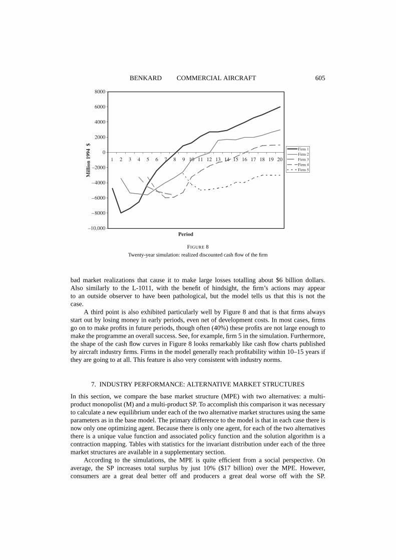
BENKARD COMMERCIAL AIRCRAFT 605
1 2 3 4 5 6 7 8 9 10 11 12 13 14 15 16 17 18 19 20
Period
Mill
ion
1994
$ Firm 1 Firm 2 Firm 3 Firm 4 Firm 5
–10,000
–8000
–6000
–4000
–2000
0
2000
4000
6000
8000
FIGURE 8
Twenty-year simulation: realized discounted cash flow of the firm
bad market realizations that cause it to make large losses totalling about $6 billion dollars.Also similarly to the L-1011, with the benefit of hindsight, the firm’s actions may appearto an outside observer to have been pathological, but the model tells us that this is not thecase.
A third point is also exhibited particularly well byFigure8 and that is that firms alwaysstart out by losing money in early periods, even net of development costs. In most cases, firmsgo on to make profits in future periods, though often (40%) these profits are not large enough tomake the programme an overall success. See, for example, firm 5 in the simulation. Furthermore,the shape of the cash flow curves inFigure8 looks remarkably like cash flow charts publishedby aircraft industry firms. Firms in the model generally reach profitability within 10–15 years ifthey are going to at all. This feature is also very consistent with industry norms.
7. INDUSTRY PERFORMANCE: ALTERNATIVE MARKET STRUCTURES
In this section, we compare the base market structure (MPE) with two alternatives: a multi-product monopolist (M) and a multi-product SP. To accomplish this comparison it was necessaryto calculate a new equilibrium under each of the two alternative market structures using the sameparameters as in the base model. The primary difference to the model is that in each case there isnow only one optimizing agent. Because there is only one agent, for each of the two alternativesthere is a unique value function and associated policy function and the solution algorithm is acontraction mapping. Tables with statistics for the invariant distribution under each of the threemarket structures are available in a supplementary section.
According to the simulations, the MPE is quite efficient from a social perspective. Onaverage, the SP increases total surplus by just 10% ($17 billion) over the MPE. However,consumers are a great deal better off and producers a great deal worse off with the SP.

606 REVIEW OF ECONOMIC STUDIES
The monopolist, on the other hand, provides much lower social welfare than either the SP orthe MPE, at great expense to consumers.25
While the SP does have the lowest production costs on average, surprisingly the welfareimprovements from the SP are not driven primarily by lower marginal costs through learning assuggested by the theoretical models (e.g.Dasgupta and Stiglitz, 1988). Given the market size andthe number of aircraft produced, in all three cases learning efficiencies are largely exhausted atthe chosen output levels. Instead, welfare gains under the SP result primarily from more standardsources. The SP sets price approximately equal to marginal cost and produces about 40% moretotal output per period on average than the competitive firms. The competitive firms in turnproduce about 2·5 times as much total output as the monopolist. The competitive firms achievethis higher output primarily through a greater number of products, which results in the leastefficient production (due to learning) of the three, confirming the findings of the theory literature.However, this cost effect is so small in practice that it is swamped by the output effect.
This is an interesting finding as it suggests that the welfare issues concentrated on bythe theory literature are not the first-order effects. It suggests that, rather than worrying aboutproductive efficiency, aircraft industry policy should instead attempt to ensure that the industrymaintains high enough current output per product.
The second area of welfare savings under the SP results from concentrating output amongjust 2·4 firms on average, as compared with 3·8 in the competitive case, which leads toapproximately a 30% reduction in new product investment. In the competitive case there is excessinvestment in development of new planes and wasted investment in learning to produce theseproducts efficiently.
8. POLICY EXPERIMENT: RESTRICTING CONCENTRATION
In a recent article,The New York Timesreferred to Boeing as “essentially a government-sanctioned monopoly”.26 Theoretically, there is reason to believe that high concentration maybe socially beneficial in industries with strong learning curves. In the absence of perfect spill-overs of experience between firms, it is always cost-minimizing to concentrate production asmuch as possible. However, the standard welfare reducing effects of monopoly are also present:in an unconstrained monopoly there tend to be fewer products and lower total production, bothof which reduce welfare.
An advantage to having such a detailed model is that it becomes possible to evaluate whicheffect will dominate in this particular industry, and hence to determine whether the current policyis the correct one. Specifically, we consider alternative anti-trust policies under which firms arepunished if they become “too large” as measured by the industry one-firm concentration ratio (aper se restriction on concentration as considered inDasgupta and Stiglitz(1988)). Under such apolicy no single firm will choose to produce more than a certain percentage of the aircraft sold ina given year. Note that with the policy in place equilibrium strategies differ from those describedabove. Firms know that the policy exists and therefore, since the policy changes pay-offs incertain states, equilibrium strategies must also change. Thus, in order to evaluate alternativepolicies it was necessary to re-solve the model for a new equilibrium in each case.27
25. Note that it is well known that logit-based models tend to imply large amounts of welfare from each product.However, since our interest is in welfare comparisons across cases, and any tendency to overestimate welfare should becomparable across cases, the comparisons should be valid. Furthermore, the high price elasticities in our model shouldmitigate this tendency somewhat.
26. New York Times, “Aircraft Giant Tries to Recover From Hard Landing” (14 November, 1997).27. In cases of outright monopoly, we assumed that the firm would be a regulated monopolist that would make
zero current profit. In equilibrium such states were reached only 0·01% of the time so this assumption has no effect onthe results.

BENKARD COMMERCIAL AIRCRAFT 607
TABLE 7
Statistics from10,000industry simulations under alternativepolicies
Maximum concentration: 100% 60% 51%
Concentration ratios: (Invariant distribution)1-Firm/plane 0·396 0·392 0·385S.D. 0·102 0·094 0·081
2-Firm/plane 0·692 0·690 0·688S.D. 0·109 0·107 0·103
Consumer surplus:Mean 135,373 134,917 133,895S.D. 7040 7268 7488
Producer surplus:Mean 42,335 42,306 42,320S.D. 3769 3776 3785
Total surplus:Mean 177,708 177,223 176,215S.D. 10,441 10,645 10,832
Table7 lists summary statistics drawn from industry simulations under the base case (norestriction) and two alternative policies. Simulations were initiated at the observed industrystructure for 1994 and use identical random draws for each policy. The experiment is thusanalogous to implementation of the given policy alternative beginning in that year. Figuresreported are present discounted values from 10,000 simulations of 200 periods each.
The results show that the impact of the two alternative policies on the predicted distributionof concentration ratios is only slight. The effect of the concentration restriction policy seems tobe largely limited to those states in which the policy actually binds, without having too great animpact on other states.Table7 also shows that the consumer and producer surplus distributionsare lower the stronger the policy alternative. However, differences are quite small compared withthe variance in these distributions making it difficult to conclude how harmful the policies are.Table8 shows the distribution of welfare gains/losses across the 10,000 simulations, making itclear that welfare losses are in fact systematic. Both policies reduce consumer surplus and totalsurplus in over 90% of the simulations. Mean total harm in the 51% policy is 0·9%, or $1·5billion in present value terms.
The concentration restriction primarily binds in states where one firm has high quality andlow cost and the others do not. In these states, the primary effect of the policy is to restrict thedominant firm’s output. Within the period, the policy has a negative effect on consumer surplus byreducing the production of the efficient dominant firm. There is also an opposing positive effectbecause the policy causes weaker firms to react by increasing their output. These two within-period effects also have dynamic implications since the dominant firm is less likely to remain alow-cost producer while weaker firms are more likely to move down their learning curves. Theevidence inTable8 suggests that once all effects are accounted for, both alternative policies leadto welfare losses overall.
Due to the richness of the model, there are a wide distribution of results from the policy.While welfare losses occur in over 90% of the simulations, in the best outcome of the 10,000simulations the 60% policy improves total welfare by approximately 12% ($19 billion). Thereason for this outcome is straightforward. There are some sequences of quality draws in whichthe firm that is dominant in the market at the start of the simulations receives bad draws onquality very early, while smaller firms receive good ones. In such sequences, a government

608 REVIEW OF ECONOMIC STUDIES
TABLE 8
Distribution of harm under alternativepolicies
Maximum concentration: 60% 51%
Consumer surplus harm:Mean 457 1478S.D. 1132 1998% Positive 95% 94%
Producer surplus harm:Mean 28·5 14·6S.D. 543 916% Positive 31% 33%
Total surplus harm:Mean 485 1493S.D. 1479 2580% Positive 94% 93%
Mean consumer harm: 0·4% 1·1%Mean producer harm: 0·1% 0·0%Mean total harm: 0·3% 0·9%
policy that hurts this dominant firm in early periods and helps smaller ones is welfare enhancingbecause it helps to reduce the costs of the future dominant firms. Of course there is no way that agovernment could possibly foresee this occurrence. Moreover, there also exist sequences wherethe opposite occurs. In one case, the 60% restriction results in a 14% ($22 billion) welfare loss.The conclusion that a concentration restriction would be welfare reducing thus holds only inexpectation. As noted inTable8, approximately 6–8% of the time such a policy would increasewelfare. This result is quite intuitive and underscores the richness of the overall model.
According to the surplus figures inTable8, producers as a whole are hurt very little by thepolicy. This result may at first seem counter-intuitive since anti-trust policy is usually thoughtof as pro-consumer. However, due to the presence of learning curves, concentrating productionlowers cost far enough that consumers may actually experience lower prices in situations whereconcentration is high. Furthermore, the conclusion that the policy does not harm producers doesnot account for the fact that the distribution of the policy’s effects is highly skewed. All producerlosses from the policy in any given period are experienced by only one firm. Thus, if such apolicy were proposed, according to the model we should expect the airlines and the dominantfirm to oppose the policy and weaker competing firms to support it.
Finally, note that in evaluating this policy we have implicitly kept firms’ investment inproduct quality fixed because we have not changed the Markov processes for quality. In actuality,since the concentration restriction reduces producer surplus in high quality states, investment inquality would likely fall on average under the policy. In that case, since producers do not accountfor the social benefit of increased investment, it also seems likely that further harm would resultfrom the policy, so that the results actually represent a lower bound to the harm distribution.
9. ROBUSTNESS
In order to evaluate the robustness of the results,Table 9 shows simulations under severalalternative parametrizations of the model. In addition to the base case, we solved the modelwith lower and higher discount factors, and lower and higher entry cost distributions. These areboth important dynamic parameters for which there was little available data.

BENKARD COMMERCIAL AIRCRAFT 609
TABLE 9
Invariant distribution under alternative parametrizations
Base xl1 = B$2·0 xl
1 = B$3·0
Model: case β = 0·90 β = 0·95 xh1 = B$3·0 xh
1 = B$4·0
Concentration ratios:1-Plane 0·40 0·44 0·39 0·39 0·40S.D. 0·10 0·12 0·10 0·10 0·11
2-Plane 0·69 0·76 0·68 0·69 0·70S.D. 0·11 0·12 0·10 0·10 0·11
Market size:No. of firms 3·8 3·3 3·9 3·8 3·7S.D. 0·4 0·6 0·4 0·4 0·5
Avg. quantity per period:Small 168 171 115 142 192Medium 60 38 92 81 33Large 4 4 34 12 3
Avg. price per unit:Small 66·2 67·9 65·5 65·9 66·5Medium 81·4 83·9 80·6 81·1 81·9Large 104·6 107·3 103·4 104·1 105·5
Avg. MC per unit:Small Lowest= 47·3 50·6 50·2 50·6 50·6 50·5Medium Lowest= 61·6 65·1 64·8 65·3 65·2 65·2Large Lowest= 83·1 86·9 86·2 87·3 87·1 86·7
Avg. (price/MC): 1·24 1·28 1·21 1·22 1·25
(Avg. price)/(Avg. TC): 1·19 1·24 1·15 1·18 1·19
New product investment per period:Mean 391 313 463 347 427S.D. 74 64 88 66 81
The results do not change qualitatively across any of the five parametrizations. However, thetable shows that the results are sensitive to the discount factor in one respect. When the discountfactor is higher, there is more entry in general and particularly more entry of the larger aircrafttypes. The reason for this is that entry in the aircraft industry always involves up-front losses withoffsetting profits that occur starting several years into the future. Higher discount factors help tomake entry in general more profitable by increasing the weight placed on the future. For largerplane types the effect appears stronger in the simulations because the larger plane types were onaverage closer to the margin of profitability.
Another feature of the discount factor runs is that the higher the discount factor, the morecompetitive the market becomes, with lower mark-ups and prices. This happens both becausethere is more entry, and because with higher discount factors the future benefit of faster learningin the present has greater weight, which leads to greater present production and lower mark-ups.In our opinion, the most reasonable values of the annual discount factor are theβ = 0·925and 0·95 cases. The only predictions of the model that change in theβ = 0·95 case vs. thebase case are that the model predicts a higher percentage of large planes and slightly lowermark-ups.
The two parametrizations with lower and higher entry costs are very similar to the base caseruns, with the expected effects of slightly more and slightly less entry, respectively.

610 REVIEW OF ECONOMIC STUDIES
10. CONCLUSIONS
This paper represents a first attempt at modelling an industry empirically using a dynamicoligopoly model with fully specified dynamics. We believe that this is an important problem forthe I.O. literature. Such an approach is critical to understanding strategic interaction and optimalpolicies in many industries.
Despite several simplifying assumptions, we find that the dynamic model predicts manyunusual aspects of the historical data well, particularly the persistent pricing of aircraft belowthe level of static marginal cost. The model also replicates many aspects of observed industrydynamics, including entry, exit, concentration ratios, plane value and plane type distributions.This evidence provides tentative support for the use of this class of dynamic models in empiricalwork more generally as these features of the industry could not be replicated with a static model.
At the same time, the aircraft industry is one of the simpler cases to work with becausethe small number of firms and products in the industry provide some relief from the curse ofdimensionality. And yet, even in this case many simplifying assumptions were necessary andstill the computational burden of the problem was found to be quite high. In order to applythe dynamic oligopoly framework to larger problems in the future, it may be necessary to findfaster computational algorithms. However, there may also be extensions to the general class ofmulti-agent dynamic models used here that would allow application to other more complex andhigher dimensional industries. Such extensions may include modelling several dominant firmsindividually and treating remaining firms as acting together through one combined agent. Inmany industries where there are only a few leading firms and a large number of “fringe” firms,such an assumption would not be unreasonable.
Having such a detailed model is a great advantage because it is well suited to analysingvarious policies by simply re-solving the model with alternative institutions in place. We haveevaluated three alternative market structures, with results suggesting that the single-productMPE is on average quite efficient from a social perspective. We also evaluated a policy thatwould restrict one-firm concentration in the aircraft industry, with the conclusion that such apolicy would reduce total welfare with high probability. Both of these policy evaluations suggestcaution with respect to government intervention in the aircraft industry. However, the model alsosuggests that an uncontested monopolist producer would lead to a large loss in social efficiency,an outcome that should be avoided if possible.
With some simple extensions, the model could also be extended to look at other anti-trust alternatives such as the break-up of a multi-product firm, regulation strategies, and variousstrategic trade policies, all of which are of current relevance in the commercial aircraft industry.With some further extensions, such as the explicit modelling of the firm’s investment in productquality, the effects of R&D subsidies could also be considered. None of these types of policysimulations would be possible without a fully specified model.
Acknowledgements. I would like to thank Ariel Pakes, Steven Berry, Donald Andrews and John Rust for theirinvaluable advice. I also thank Daniel Ackerberg, Patrick Bajari, Tom Crawford, Dennis Epple, Gautam Gowrisankaran,Phillip Leslie, Michael Riordan, the editor, three anonymous referees and many seminar participants for their helpfulcomments. Financial assistance was provided by the Alfred P. Sloan Foundation.
REFERENCES
ALCHIAN, A. (1963), “Reliability of Progress Curves in Airframe Production”,Econometrica, 31 (4), 679–694.ANDREWS, D. W. K. (1991), “Heteroskedasticity and Autocorrelation Consistent Covariance Matrix Estimation”,
Econometrica, 59 (3), 817–858.ARGOTE, L. and EPPLE, D. (1990), “Learning Curves in Manufacturing”,Science, 247, 924.ASHER, H. (1956)Cost–Quantity Relationships in the Airframe Industry, R-291 (Santa Monica, CA: The RAND
Corporation).

BENKARD COMMERCIAL AIRCRAFT 611
BALDWIN, R. and KRUGMAN, P. (1988), “Industrial Policy and International Competition in Wide-Bodied JetAircraft”, in R. E. Baldwin (ed.)Trade Policy and Empirical Analysis(University of Chicago Press for the NBER)45–71.
BENKARD, C. L. (1996), “A Simple Extension of Logit to Multiple Purchases and Application to CommercialAirframes” (Mimeo, Stanford University).
BENKARD, C. L. (2000), “Learning and Forgetting: The Dynamics of Commercial Aircraft Production”,AmericanEconomic Review, 90 (4), 1034–1054.
BERRY, S. (1994), “Estimating Discrete-Choice Models of Product Differentiation”,RAND Journal of Economics,25 (2), 242–262.
BERRY, S. and PAKES, A. (1993), “Some Applications and Limitations of Recent Advances in Empirical IndustrialOrganization: Merger Analysis”,American Economic Review, 83 (2), 247–252.
CABRAL, L. M. B. and RIORDAN, M. (1994), “The Learning Curve, Market Dominance, and Predatory Pricing”,Econometrica, 62 (5), 1115–1140.
DASGUPTA, P. and STIGLITZ, J. (1988), “Learning-by-Doing, Market Structure and Industrial and Trade Policies”,Oxford Economic Papers, 40, 246–268.
ERICSON, R. and PAKES, A. (1995), “Markov-Perfect Industry Dynamics: A Framework for Empirical Work”,Reviewof Economic Studies, 62 (1), 53–83.
FERSHTMAN, C. and PAKES, A. (2000), “A Dynamic Oligopoly with Collusion and Price Wars”,RAND Journal ofEconomics, 31 (2), 207–236.
FUDENBURG, D. and TIROLE, J. (1983), “Learning-by-Doing and Market Performance”,Bell Journal of Economics,14, 522–530.
GOWRISANKARAN, G. (1999), “A Dynamic Model of Endogenous Horizontal Mergers”,RAND Journal of Economics,30 (1), 56–83.
GOWRISANKARAN, G. and TOWN, R. (1997), “Dynamic Equilibrium in the Hospital Industry”,Journal of Economicsand Management Strategy, 6 (1), 45–74.
GULLEDGE, T. R. and WOMER, N. K. (1986)The Economics of Made-to-Order Production(New York: Springer).HENDEL, I. (1999), “Estimating Multiple-Discrete Choice Models: An Application to Computerization Returns”,Review
of Economic Studies, 66 (2), 423–446.JUDD, K. L. (1996), “Cournot Versus Bertrand: A Dynamic Resolution” (Working Paper, Hoover Institution).KLEPPER, G. (1990), “Entry into the Market for Large Transport Aircraft”,European Economic Review, 34, 775–803.MASKIN, E. and TIROLE, J. (1988a), “A Theory of Dynamic Oligopoly, I: Overview and Quantity Competition with
Large Fixed Costs”,Econometrica, 56 (3), 549–569.MASKIN, E. and TIROLE, J. (1988b), “A Theory of Dynamic Oligopoly, II: Price Competition, Kinked Demand Curves,
and Edgeworth Cycles”,Econometrica, 56 (3), 571–599.NEVEN, D. and SEABRIGHT, P. (1995), “European Industrial Policy: The Airbus Case”,Economic Policy, 313–358.NEWHOUSE, J. (1982)The Sporty Game(New York: Alfred A. Knopf Inc.).New York Times(1997) “Aircraft Giant Tries to Recover From Hard Landing” (14 November).PAKES, A. and MCGUIRE, P. (1994), “Computing Markov Perfect Nash Equilibria: Numerical Implications of a
Dynamic Differentiated Product Model”,RAND Journal of Economics, 25 (4), 555–589.PAKES, A. and MCGUIRE, P. (2001), “Stochastic Approximation for Dynamic Models: Markov Perfect Equilibrium
and the ‘Curse’ of Dimensionality”,Econometrica, 69 (5), 1261–1281.REINHARDT, U. E. (1973), “Break-Even Analysis for Lockheed’s Tri Star: An Application of Financial Theory”,
Journal of Finance, 28 (4), 821–838.RESETAR, S., ROGERS, J. and HESS, R. (1991)Advanced Airframe Structural Materials: A Primer and Cost
Estimating Methodology, Prepared for the United States Air Force, R-4016-AF (Santa Monica, CA: The RANDCorporation).
SEITZ, F. and STEELE, L. (1985)The Competitive Status of the U.S. Civil Aviation Manufacturing Industry(Washington,DC: National Academy Press).
SPENCE, A. M. (1981), “The Learning Curve and Competition”,Bell Journal of Economics, 12, 49–70.TYSON, L. D. (1992)Who’s Bashing Whom? Trade Conflict in High-Technology Industries(Washington, DC: Institute
for International Economics).Wall Street Journal(1999), “Flight of Fancy: Airbus Prepares to ‘Bet the Company’ as It Builds a Huge New Jet”,
(November) A1.WRIGHT, T. P. (1936), “Factors Affecting the Cost of Airplanes”,Journal of the Aeronautical Sciences, 3, 122–128.