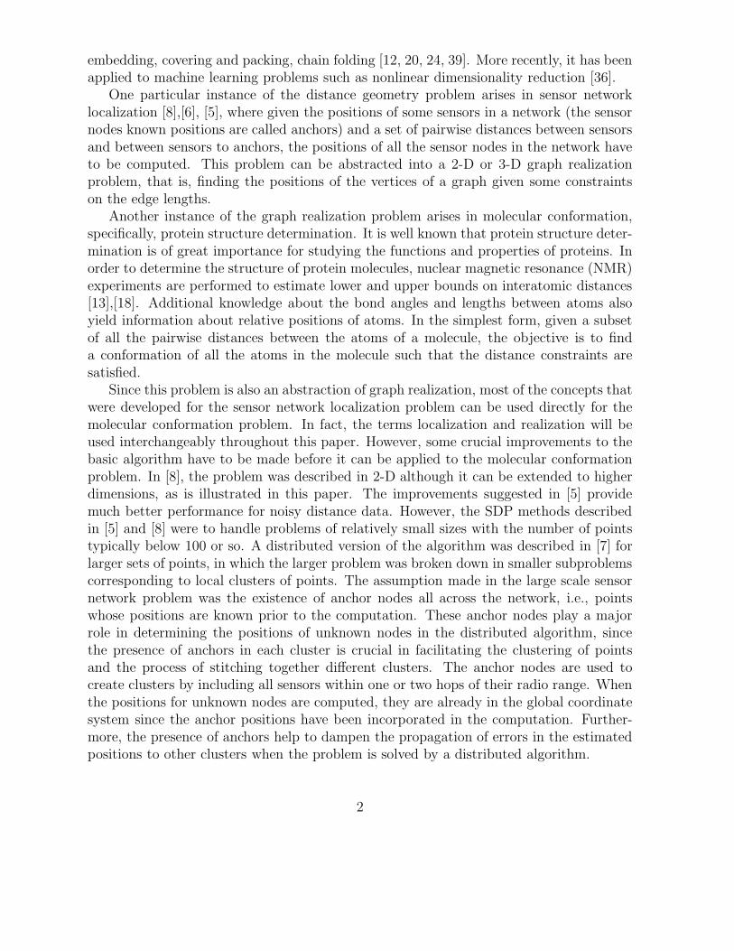
A Distributed SDP Approach forLarge-scale Noisy Anchor-free Graph

Realization with Applications to MolecularConformation

Pratik Biswas∗, Kim-Chuan Toh †, Yinyu Ye ‡

October 16, 2007

Abstract

We propose a distributed algorithm for solving Euclidean metric realization prob-lems arising from large 3D graphs, using only noisy distance information, and with-out any prior knowledge of the positions of any of the vertices. In our distributedalgorithm, the graph is first subdivided into smaller subgraphs using intelligent clus-tering methods. Then a semidefinite programming relaxation and gradient searchmethod is used to localize each subgraph. Finally, a stitching algorithm is usedto find affine maps between adjacent clusters and the positions of all points in aglobal coordinate system are then derived. In particular, we apply our method tothe problem of finding the 3D molecular configurations of proteins based on a lim-ited number of given pairwise distances between atoms. The protein molecules, allwith known molecular configurations, are taken from the Protein Data Bank. Ouralgorithm is able to reconstruct reliably and efficiently the configurations of largeprotein molecules from a limited number of pairwise distances corrupted by noise,without incorporating domain knowledge such as the minimum separation distanceconstraints derived from van der Waals interactions.

1 Introduction

Semidefinite programming (SDP) relaxation techniques can be used for solving a widerange of Euclidean distance geometry problems, such as data compression, metric-space

∗Electrical Engineering, Stanford University, Stanford, CA 94305. E-mail: pbiswas@stanford.edu.†Department of Mathematics, National University of Singapore, 2 Science Drive 2, Singapore 117543,

Singapore. E-mail: mattohkc@nus.edu.sg.‡Management Science and Engineering and, by courtesy, Electrical Engineering, Stanford University,

Stanford, CA 94305. E-mail: yinyu-ye@stanford.edu.

1

embedding, covering and packing, chain folding [12, 20, 24, 39]. More recently, it has beenapplied to machine learning problems such as nonlinear dimensionality reduction [36].

One particular instance of the distance geometry problem arises in sensor networklocalization [8],[6], [5], where given the positions of some sensors in a network (the sensornodes known positions are called anchors) and a set of pairwise distances between sensorsand between sensors to anchors, the positions of all the sensor nodes in the network haveto be computed. This problem can be abstracted into a 2-D or 3-D graph realizationproblem, that is, finding the positions of the vertices of a graph given some constraintson the edge lengths.

Another instance of the graph realization problem arises in molecular conformation,specifically, protein structure determination. It is well known that protein structure deter-mination is of great importance for studying the functions and properties of proteins. Inorder to determine the structure of protein molecules, nuclear magnetic resonance (NMR)experiments are performed to estimate lower and upper bounds on interatomic distances[13],[18]. Additional knowledge about the bond angles and lengths between atoms alsoyield information about relative positions of atoms. In the simplest form, given a subsetof all the pairwise distances between the atoms of a molecule, the objective is to finda conformation of all the atoms in the molecule such that the distance constraints aresatisfied.

Since this problem is also an abstraction of graph realization, most of the concepts thatwere developed for the sensor network localization problem can be used directly for themolecular conformation problem. In fact, the terms localization and realization will beused interchangeably throughout this paper. However, some crucial improvements to thebasic algorithm have to be made before it can be applied to the molecular conformationproblem. In [8], the problem was described in 2-D although it can be extended to higherdimensions, as is illustrated in this paper. The improvements suggested in [5] providemuch better performance for noisy distance data. However, the SDP methods describedin [5] and [8] were to handle problems of relatively small sizes with the number of pointstypically below 100 or so. A distributed version of the algorithm was described in [7] forlarger sets of points, in which the larger problem was broken down in smaller subproblemscorresponding to local clusters of points. The assumption made in the large scale sensornetwork problem was the existence of anchor nodes all across the network, i.e., pointswhose positions are known prior to the computation. These anchor nodes play a majorrole in determining the positions of unknown nodes in the distributed algorithm, sincethe presence of anchors in each cluster is crucial in facilitating the clustering of pointsand the process of stitching together different clusters. The anchor nodes are used tocreate clusters by including all sensors within one or two hops of their radio range. Whenthe positions for unknown nodes are computed, they are already in the global coordinatesystem since the anchor positions have been incorporated in the computation. Further-more, the presence of anchors help to dampen the propagation of errors in the estimatedpositions to other clusters when the problem is solved by a distributed algorithm.

2

Without anchors, we need alternative methods to cluster the points and to stitch theclusters together. In this paper, we propose a distributed algorithm for solving largescale noisy anchor-free Euclidean metric realization problems arising from 3-D graphs, toaddress precisely the issues just mentioned. In the problem considered here, there areno a priori determined anchors, as is the case in the molecular conformation problem.Therefore the strategy of creating local clusters for distributed computation is different.We perform repeated matrix permutations on the sparse distance matrix to form localclusters within the structure. The clusters are built keeping in mind the need to maintaina reasonably high degree of overlap between adjacent clusters, i.e., there should be enoughcommon points considered between adjacent clusters. This is used to our advantage whenwe combine the results from different clusters during the stitching process.

Within each cluster, the positions of the points are first estimated by solving an SDPrelaxation of a non-convex minimization problem seeking to minimize the sum of errorsbetween given and estimated distances. A gradient-descent minimization method, firstdescribed in [23], is used as a postprocessing step, after the SDP computation to furtherreduce the estimation errors. The refinement of errors by a local optimization method isespecially important as there may not be enough distance data in a cluster, or the noise inthe distance measures may be too high, to determine a unique realization in the requireddimensional space. In that case, the SDP solution is in a higher dimensional space,and a simple projection of that solution into a lower dimensional space does not yieldcorrect positions. Fortunately, it can often serve as a good starting iterate for a localoptimization method to obtain a lower dimensional realization that satisfies the givendistance constraints. After the gradient-descent postprocessing step, poorly estimatedpoints within each cluster are isolated and they are recomputed when more points arecorrectly estimated.

The solution of each individual cluster yields different orientations in their local coor-dinate systems since there are no anchors to provide global coordinate information. Thelocal configuration may be rotated, reflected, or translated while still respecting the dis-tance constraints. This was not a problem in the case when anchors were available, as theywould perform the task of ensuring that each cluster follows the same global coordinatesystem. Instead in this paper, we use a least squares based affine mapping between localcoordinates of common points in overlapping clusters to create a coherent conformationof all points in a global coordinate system.

We test our algorithm on protein molecules of varying sizes and configurations. Theprotein molecules, all with known molecular configurations, are taken from the ProteinData Bank [4]. Our algorithm is able to reliably reconstruct the configurations of largemolecules with thousands of atoms quite efficiently and accurately based on given upperand lower bounds on limited pairwise distances between atoms. To the best of our knowl-edge, there are no computational results reported in existing literature for determiningmolecular structures of this scale by using only sparse and noisy distance information.However, there is still room for improvement in our algorithm in the case of very sparse

3

or highly noisy distance data.For simplicity, our current SDP based distributed algorithm does not incorporate

the lower constraints generated from van der Waals (VDW) interactions between atoms.But such constraints can naturally be incorporated into the SDP model. Given that ourcurrent algorithm performs quite satisfactorily without the VDW lower bound constraints,we are optimistic that with the addition of such constraints and other improvements inthe future, our algorithm would perform well even for the very difficult case of highlynoisy and very sparse distance data.

Section 2 of this paper describes related work in distance geometry, SDP relaxationsand molecular conformation, and attempts to situate our work in that context. Section 3elucidates the distance geometry problem and the SDP relaxation models. A preliminarytheory for anchor-free graph realization is also developed. In particular, regularizationideas to improve the SDP solution quality in the presence of noise are discussed. Theintelligent clustering and cluster stitching algorithms are introduced in Section 4 and 5respectively. Postprocessing techniques to refine the SDP estimated positions are dis-cussed in Section 6. Section 7 describes the complete distributed algorithm. Section 8discusses the performance of the algorithm on protein molecules from the Protein DataBank [4]. Finally in Section 9, we conclude with a summary of the paper and outlinesome work in progress to improve our distributed algorithm.

2 Related work

Owing to their large applicability, a lot of attention has been paid to Euclidean distancegeometry problems. The use of SDP relaxations to solve this class of problems involvesrelaxing the nonconvex quadratic distance constraints into convex linear constraints overthe cone of positive semidefinite matrices. It is illustrated through sensor network prob-lems in [8]. Similar relaxations have also been developed in [2], [22] and [36].

As the number of points and pairwise distances increase, it becomes computationallyintractable to solve the entire SDP in a centralized fashion. With special focus on anchoredsensor network localization problems, a distributed technique is proposed in [7]. Thisinvolves solving smaller clusters of points in parallel and using information from points indifferent clusters in subsequent iterations to refine the solutions.

Building on the ideas in [7], the authors in [11],[21] proposed an adaptive rule basedclustering strategy to sequentially divide a global anchored graph localization problem (in2-dimension) into a sequence of subproblems. The technique in localizing each subproblemis similar to that in [7], but the clustering and stitching strategies are different. It isreported that the improved techniques can localize anchored graphs very efficiently andaccurately.

Interestingly, the SDP relaxation method not only solves for unknown points, thesolution matrix also provides an error measure for each estimation. Furthermore, thedual of the SDP relaxation also gives insights into the localizability of the given set of

4

points. In fact, the issue of localizability, that is, the existence of a unique configurationof points satisfying the distance constraints is closely linked to the rigidity of the graphstructure underlying the set of points. These issues are explored in detail in [28].

Many approaches have been developed for the molecular distance geometry problem.An overall discussion of the methods and related software is provided in [40]. Some of theapproaches are briefly described below.

When the exact distances between all pairs of n points are given, a valid configurationcan be obtained by computing the eigenvalue decomposition of an (n−1)×(n−1) matrix(which can be obtained through a linear transformation of the squared distance matrix).Note that if the configuration of n points can be realized in a d-dimensional space, thenthe aforementioned matrix must have rank d, and the eigenvectors corresponding to thed nonzero eigenvalues give a valid configuration. So a decomposition can be found anda configuration constructed in O(n3) arithmetic operations. The EMBED algorithm [13]exploits this idea for sparse and noisy distances by first performing bound smoothing,that is, preprocessing the available data to remove geometric inconsistencies and findingvalid estimates for unknown distances. Then a valid configuration is obtained throughthe eigenvalue decomposition of the inner product matrix and the estimated positions arethen used as the starting iterate for local optimization methods on certain nonlinear leastsquares problems.

Classical multidimensional scaling (MDS) is the general class of methods that takes in-exact distances as input, and extracts a valid configuration from them based on minimizingthe discrepancy between the inexact measured distances and the distances correspondingto the estimated configuration. The inexact distance matrix is referred to as a dissimilar-ity matrix in this framework. Since the distance data is also incomplete, the problem alsoinvolves completing the partial distance matrix. The papers [32], [33], [34] consider thisproblem of completing a partial distance matrix, as well as the more general problem offinding a distance matrix of prescribed embedding dimension that satisfies specified lowerand upper bounds, for use in MDS based algorithms. In [33], good conformation resultswere reported for molecules with a few hundred atoms each under the condition that allthe pairwise distances (specified in the form of lower and upper bounds with a gap of0.02A) below 7A were given.

Also worth noting in this regard is the distance geometry program APA describedin [27], that applies the idea of a data box, a rectangular parallelepiped of dissimilaritymatrices that satisfy some given upper and lower bounds on distances. An alternatingprojection based optimization technique is then used to solve for both a dissimilaritymatrix that lies within the data box, and a valid embedding of the points, such that thediscrepancy between the dissimilarity matrix and the distances from the embedding areminimized.

The ABBIE software package [19], on the other hand, exploits the concepts of graphrigidity to solve for smaller subgraphs of the entire graph defined by the points and dis-tances and finally combining the subgraphs to find an overall configuration. It is especially

5

advantageous to solve for smaller parts of the molecule and to provide certificates confirm-ing that the distance information is not enough to ascertain certain atoms. Our approachtries to retain these advantages by solving the molecule in a distributed fashion, that is,solving smaller clusters and later assembling them together.

Some global optimization methods attempt to attack the problem of finding a confor-mation which fits the given data as a large nonlinear least squares problem. For example,a global smoothing and continuation approach is used in the DGSOL algorithm [25]. Toprevent the algorithm from getting stuck at one of the large number of possible localminimizers, the nonlinear least squares problem (with an objective that is closely relatedto the refinement stage of the EMBED algorithm) is mollified to smoother functions so asto increase the chance of locating the global minimizer. However, it can still be difficultto find the global minimizer from various random starting points, especially with noisydistance information. More refined methods that try to circumvent such difficulties havealso been developed in [26], though with limited success.

Another example is the GNOMAD algorithm [37], also a global optimization method,which takes special care to satisfy the physically inviolable minimum separation distance,or van der Waals (VDW) constraints. For GNOMAD, the VDW constraints are crucial inreducing the search space in the case of very sparse distance data. Obviously, the VDWconstraints can easily be incorporated into any molecular conformation problem that ismodelled by an optimization problem. In [37], the success of the GNOMAD algorithmwas demonstrated on 4 molecules (the largest one has 5591 atoms) under the assumptionthat 30-70% of the exact pairwise distances below 6A were given. In addition, the givendistances included those from covalently bonded atoms and those between atoms thatshare covalent bonds with the same atom.

Besides optimization based methods, there are geometry based methods proposed forthe molecular conformation problem. The effectiveness of simple geometric build up (alsoknown as triangulation) algorithms has been demonstrated in [14] and [38] for moleculeswhen exact distances within a certain cut-off radius are all given. Basically, this approachinvolves using the distances between an unknown atom and previously determined neigh-boring atoms to find the coordinates of the unknown atom. The algorithm progressivelyupdates the number of known points and uses them to compute points that have not yetbeen determined. However, the efficacy of such methods for large molecules with verysparse and noisy data has not yet been demonstrated.

In this paper, we will attempt to find the structures of molecules with sizes varyingfrom hundreds to several thousands of atoms, given only upper and lower bounds onsome limited pairwise distances between atoms. The approach described in this paper alsoperforms distance matrix completion, similar to some of the methods described above. Theextraction of the point configuration after matrix completion is still the same as the MDSmethods. The critical difference lies in the use of an SDP relaxation for completing thedistance matrix. Furthermore, our distributed approach avoids the issue of intractabilityfor very large molecules by splitting the molecule into smaller subgraphs, much like the

6

ABBIE algorithm [19] and then stitching together the different clusters. Some of the atomswhich are incorrectly estimated are solved separately using the correctly estimated atomsas anchors. The latter bears some similarities to the geometric build up algorithms. Inthis way, we adapted and improved some of the techniques used in previous approaches,but also introduced new ideas generated from recent advances in SDP to attack thetwin problems of dealing with noisy and sparse distance data, and the computationalintractability of large scale molecular conformation.

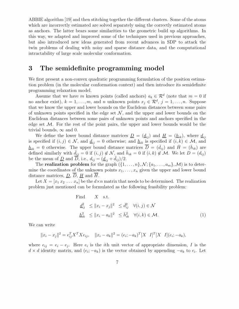
3 The semidefinite programming model

We first present a non-convex quadratic programming formulation of the position estima-tion problem (in the molecular conformation context) and then introduce its semidefiniteprogramming relaxation model.

Assume that we have m known points (called anchors) ak ∈ Rd (note that m = 0 ifno anchor exist), k = 1, . . . , m, and n unknown points xj ∈ Rd, j = 1, . . . , n. Supposethat we know the upper and lower bounds on the Euclidean distances between some pairsof unknown points specified in the edge set N , and the upper and lower bounds on theEuclidean distances between some pairs of unknown points and anchors specified in theedge set M. For the rest of the point pairs, the upper and lower bounds would be thetrivial bounds, ∞ and 0.

We define the lower bound distance matrices D = (dij) and H = (hik), where dij

is specified if (i, j) ∈ N , and dij = 0 otherwise; and hik is specified if (i, k) ∈ M, and

hik = 0 otherwise. The upper bound distance matrices D = (dij) and H = (hik) aredefined similarly with dij = 0 if (i, j) 6∈ N , and hik = 0 if (i, k) 6∈ M. We let D = (dij)be the mean of D and D, i.e., dij = (dij + dij)/2.

The realization problem for the graph ({1, . . . , n},N ; {a1, . . . , am},M) is to deter-mine the coordinates of the unknown points x1, . . . , xn given the upper and lower bounddistance matrices, D, D, H and H .

Let X = [x1 x2 . . . xn] be the d×n matrix that needs to be determined. The realizationproblem just mentioned can be formulated as the following feasibility problem:

Find X s.t.

d2ij ≤ ‖xi − xj‖2 ≤ d2

ij ∀(i, j) ∈ N

h2ik ≤ ‖xi − ak‖2 ≤ h2

ik ∀(i, k) ∈M. (1)

We can write

‖xi − xj‖2 = eTijX

TXeij , ‖xi − ak‖2 = (ei;−ak)T [X I]T [X I](ei;−ak),

where eij = ei − ej. Here ei is the ith unit vector of appropriate dimension, I is thed × d identity matrix, and (ei;−ak) is the vector obtained by appending −ak to ei. Let

7

Y = XT X and Z = [Y XT ; X I]. Then the problem (1) can be rewritten as:

Find Z s.t.

d2ij ≤ eT

ijY eij ≤ d2ij, ∀(i, j) ∈ N

h2ik ≤ (ei;−ak)

T Z(ei;−ak) ≤ h2ik, ∀(i, k) ∈M

Z = [Y XT ; X I], Y = XTX. (2)

The above problem (2) is unfortunately non-convex. Our method is to relax it to anSDP by relaxing the constraint Y = XT X to Y � XT X (meaning that Y − XT X ispositive semidefinite). The last matrix inequality is equivalent to (Boyd et al. [9])

Z =

(Y XT

X I

)� 0, Z symmetric.

Thus, the SDP relaxation of (2) can be written as the following standard SDP problem:

Find Z s.t.

d2ij ≤ eT

ijZeij ≤ d2ij, ∀ (i, j) ∈ N

h2ik ≤ (ei;−ak)

T Z(ei;−ak) ≤ h2ik, ∀ (i, k) ∈M

eTi Zei = 1, ∀ n + 1 ≤ i ≤ n + d

(ei + ej)T Z(ei + ej) = 2, ∀ n + 1 ≤ i < j ≤ n + d

Z � 0. (3)

Note that the last two sets of equality constraints in (3) specify that the lower-right d× dblock of Z is the identity matrix.

We note that if there are additional constraints of the form ‖xi−xj‖ ≥ L coming fromknowledge about the minimum separation distance between any 2 points, such constraintscan be included in the SDP (3) by adding inequality constraints of the form: eT

ijZeij ≥L2. In molecular conformation, the minimum separation distances corresponding to theVDW interactions are used in an essential way to reduce the search space in the atom-based constrained optimization algorithm (GNOMAD) described in [37]. The minimumseparation distance constraints are also easily incorporated in the MDS framework [27, 33].

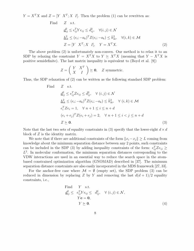
For the anchor-free case where M = ∅ (empty set), the SDP problem (3) can bereduced in dimension by replacing Z by Y and removing the last d(d + 1)/2 equalityconstraints, i.e.,

Find Y s.t.

d2ij ≤ eT

ijY eij ≤ d2ij, ∀ (i, j) ∈ N ,

Y e = 0,

Y � 0. (4)

8

This is because when M = ∅, the (1, 2) and (2, 1) block of Z are always equal to zero ifthe starting iterate for the interior-point method used to solve (3) is chosen to be so. Notethat we add the extra constraint Y e = 0 to eliminate the translational invariance of theconfiguration by putting the center of gravity of the points at the origin, i.e.,

∑ni=1 xi = 0.

Note also that in the anchor-free case, if the graph is localizable (defined in the nextsubsection), a realization X ∈ Rd×n can no longer be obtained from the (2, 1) block of Zbut needs to be computed from the inner product matrix Y by factorizing it to the formY = XT X via eigenvalue decomposition (as has been done in previous methods discussedin the literature review). In the noisy case, the inner product matrix Y would typicallyhave rank greater than d. In practice, X is chosen to be the best rank-d approximation,by choosing the eigenvectors corresponding to the d largest eigenvalues. The configurationso obtained is a rotated or reflected version of the actual point configuration.

3.1 Theory of anchor-free graph realization

In order to establish the theoretical properties of the SDP relaxation, we will considerthe cases where all the given distances in N are exact, i.e., without noise. A graphG = ({1, . . . , n}, D) is localizable in dimension d if (i) it has a realization X in Rd×n suchthat ‖xi− xj‖ = dij for all (i, j) ∈ N ; (ii) it cannot be realized (non-trivially) in a higherdimensional space. We let D = (dij) be the n × n matrix such that its (i, j) element dij

is the given distance between points i and j when (i, j) ∈ N , and zero otherwise. It isshown for the exact distances case in [28] that if the graph with anchors is localizable,then the SDP relaxation will produce a unique optimal solution Z with its (1,1) blockequal to XT X. For the anchor free case where M = ∅, it is clear that the realizationcannot be unique since the configuration may be translated, rotated, or reflected, and stillpreserve the same distances.

To remove the translational invariance, we will add an objective function to minimizethe norm of the solution in the problem formulation:

minimize∑n

j=1 ‖xj‖2

s.t. ‖xi − xj‖2 = d2ij , ∀ (i, j) ∈ N .

(5)

What this minimization does is to translate the center of gravity of the points to theorigin, that is, if xj, j = 1, ..., n, is the realization of the problem, then the realizationgenerated from the (5) will be xj − x, j = 1, ..., n, where x = 1

n

∑nj=1 xj , subject to only

rotation and reflection. The norm minimization also helps the following SDP relaxationof (5) to have bounded solutions:

minimize Trace(Y ) = I • Y

s.t. eTijY eij = d2

ij , ∀ (i, j) ∈ N ,

Y � 0,

(6)

9

where Y ∈ Sn (the space of n × n symmetric matrices), I is the identity matrix, and •denotes the standard matrix inner product. We note that a model similar to (6) is alsoproposed in [1] but with the objective function replaced by ‖Y ‖2F . The dual of the SDPrelaxation (6) is given by:

maximize∑

(i,j)∈N wijd2ij

s.t. I −∑(i,j)∈N wij · eije

Tij � 0.

(7)

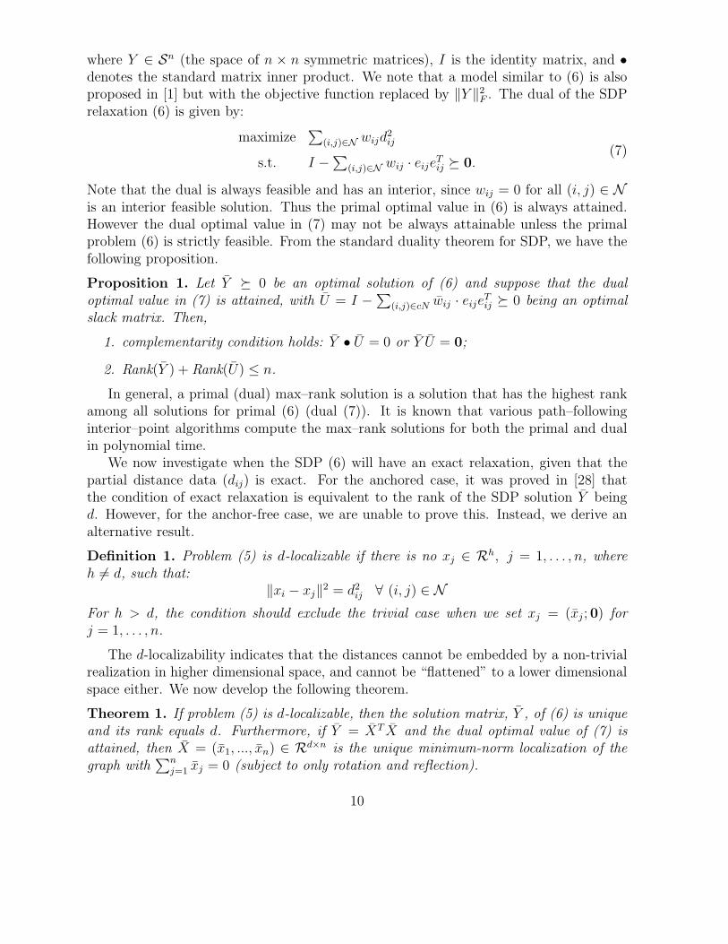
Note that the dual is always feasible and has an interior, since wij = 0 for all (i, j) ∈ Nis an interior feasible solution. Thus the primal optimal value in (6) is always attained.However the dual optimal value in (7) may not be always attainable unless the primalproblem (6) is strictly feasible. From the standard duality theorem for SDP, we have thefollowing proposition.

Proposition 1. Let Y � 0 be an optimal solution of (6) and suppose that the dualoptimal value in (7) is attained, with U = I −∑

(i,j)∈cN wij · eijeTij � 0 being an optimal

slack matrix. Then,

1. complementarity condition holds: Y • U = 0 or Y U = 0;

2. Rank(Y ) + Rank(U) ≤ n.

In general, a primal (dual) max–rank solution is a solution that has the highest rankamong all solutions for primal (6) (dual (7)). It is known that various path–followinginterior–point algorithms compute the max–rank solutions for both the primal and dualin polynomial time.

We now investigate when the SDP (6) will have an exact relaxation, given that thepartial distance data (dij) is exact. For the anchored case, it was proved in [28] thatthe condition of exact relaxation is equivalent to the rank of the SDP solution Y beingd. However, for the anchor-free case, we are unable to prove this. Instead, we derive analternative result.

Definition 1. Problem (5) is d-localizable if there is no xj ∈ Rh, j = 1, . . . , n, whereh 6= d, such that:

‖xi − xj‖2 = d2ij ∀ (i, j) ∈ N

For h > d, the condition should exclude the trivial case when we set xj = (xj ; 0) forj = 1, . . . , n.

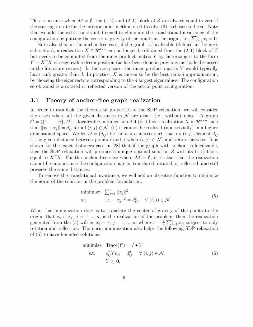
The d-localizability indicates that the distances cannot be embedded by a non-trivialrealization in higher dimensional space, and cannot be “flattened” to a lower dimensionalspace either. We now develop the following theorem.

Theorem 1. If problem (5) is d-localizable, then the solution matrix, Y , of (6) is uniqueand its rank equals d. Furthermore, if Y = XT X and the dual optimal value of (7) isattained, then X = (x1, ..., xn) ∈ Rd×n is the unique minimum-norm localization of thegraph with

∑nj=1 xj = 0 (subject to only rotation and reflection).

10

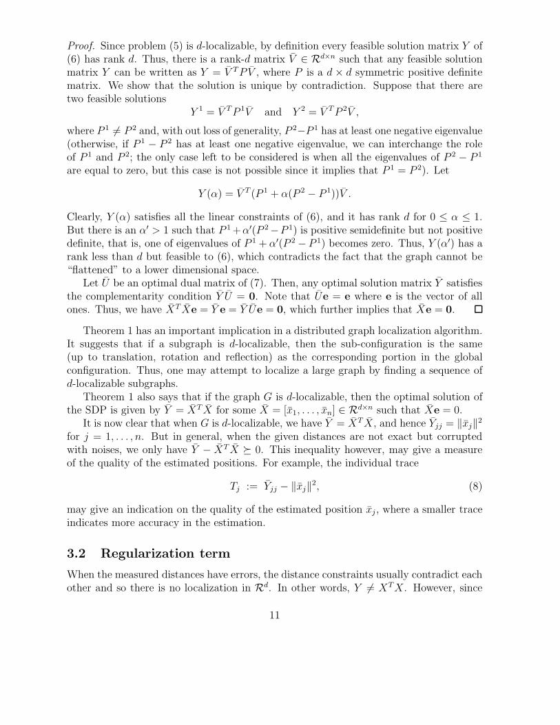
Proof. Since problem (5) is d-localizable, by definition every feasible solution matrix Y of(6) has rank d. Thus, there is a rank-d matrix V ∈ Rd×n such that any feasible solutionmatrix Y can be written as Y = V T P V , where P is a d × d symmetric positive definitematrix. We show that the solution is unique by contradiction. Suppose that there aretwo feasible solutions

Y 1 = V T P 1V and Y 2 = V T P 2V ,

where P 1 6= P 2 and, with out loss of generality, P 2−P 1 has at least one negative eigenvalue(otherwise, if P 1 − P 2 has at least one negative eigenvalue, we can interchange the roleof P 1 and P 2; the only case left to be considered is when all the eigenvalues of P 2 − P 1

are equal to zero, but this case is not possible since it implies that P 1 = P 2). Let

Y (α) = V T (P 1 + α(P 2 − P 1))V .

Clearly, Y (α) satisfies all the linear constraints of (6), and it has rank d for 0 ≤ α ≤ 1.But there is an α′ > 1 such that P 1 +α′(P 2−P 1) is positive semidefinite but not positivedefinite, that is, one of eigenvalues of P 1 + α′(P 2 − P 1) becomes zero. Thus, Y (α′) has arank less than d but feasible to (6), which contradicts the fact that the graph cannot be“flattened” to a lower dimensional space.

Let U be an optimal dual matrix of (7). Then, any optimal solution matrix Y satisfiesthe complementarity condition Y U = 0. Note that Ue = e where e is the vector of allones. Thus, we have XT Xe = Y e = Y Ue = 0, which further implies that Xe = 0.

Theorem 1 has an important implication in a distributed graph localization algorithm.It suggests that if a subgraph is d-localizable, then the sub-configuration is the same(up to translation, rotation and reflection) as the corresponding portion in the globalconfiguration. Thus, one may attempt to localize a large graph by finding a sequence ofd-localizable subgraphs.

Theorem 1 also says that if the graph G is d-localizable, then the optimal solution ofthe SDP is given by Y = XT X for some X = [x1, . . . , xn] ∈ Rd×n such that Xe = 0.

It is now clear that when G is d-localizable, we have Y = XT X, and hence Yjj = ‖xj‖2for j = 1, . . . , n. But in general, when the given distances are not exact but corruptedwith noises, we only have Y − XT X � 0. This inequality however, may give a measureof the quality of the estimated positions. For example, the individual trace

Tj := Yjj − ‖xj‖2, (8)

may give an indication on the quality of the estimated position xj , where a smaller traceindicates more accuracy in the estimation.

3.2 Regularization term

When the measured distances have errors, the distance constraints usually contradict eachother and so there is no localization in Rd. In other words, Y 6= XTX. However, since

11

the SDP approach relaxes the constraint Y = XTX into Y � XT X, it is still possibleto locate the points in a higher dimensional space (or choose a Y with a higher rank)such that they satisfy the distance constraints exactly. The optimal solution in a higherdimensional space always results in a smaller violation of the distance constraints than theone constrained in Rd. Furthermore, the ’max-rank’ property [17] implies that solutionsobtained through interior point methods for solving SDPs converge to the maximum ranksolutions. Hence, because of the relaxation of the rank requirement, the solution is “lifted”to a higher dimensional space. For example, imagine a rigid structure consisting of setof points in a plane (with the points having specified distances from each other). If weperturb some of the specified distances, the configuration may need to be readjusted bysetting some of the points outside the plane.

The above discussion leads us to the question on how to round the higher-dimensional(higher rank) SDP solution into a lower-dimensional (in this case, rank-3) solution. Oneway is to ignore the augmented dimensions and use the projection X∗ as a suboptimalsolution, which is the case in [8]. However, the projection typically leads to points getting“crowded” together. (Imagine the projection of the top vertex of a pyramid onto its base.)This is because a large contribution to the distance between 2 points could come from thedimensions we choose to ignore.

In [36], regularization terms have been incorporated to the SDP arising from kernellearning in nonlinear dimensionality reduction. The purpose is to penalize folding and tryto find a stretched map of the set of points while respecting local distance constraints.Here we propose a similar strategy to ameliorate the difficulty of crowding.

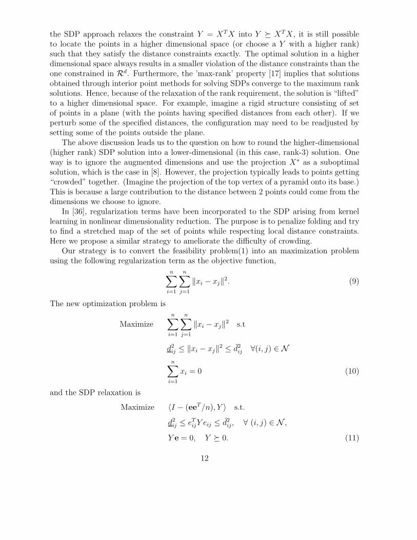
Our strategy is to convert the feasibility problem(1) into an maximization problemusing the following regularization term as the objective function,

n∑

i=1

n∑

j=1

‖xi − xj‖2. (9)

The new optimization problem is

Maximize

n∑

i=1

n∑

j=1

‖xi − xj‖2 s.t

d2ij ≤ ‖xi − xj‖2 ≤ d2

ij ∀(i, j) ∈ Nn∑

i=1

xi = 0 (10)

and the SDP relaxation is

Maximize 〈I − (eeT /n), Y 〉 s.t.

d2ij ≤ eT

ijY eij ≤ d2ij, ∀ (i, j) ∈ N ,

Y e = 0, Y � 0. (11)

12

where e is the vector of all ones. As mentioned before, the constraint∑n

i=1 xi = 0 andY e = 0 are to remove the translational invariance of the configuration of points by puttingthe center of gravity at the origin.

The addition of a regularization term penalizes folding between the points and maxi-mizes the separation between them, while still respecting local distance constraints. Theidea of regularization has also been linked to tensegrity theory and realizability of graphsin lower dimensions, see [29]. The notion of stress is used to explain this. By maximizingthe distance between some vertices in a graph, the graph gets stretched out and there isa non-zero stress induced on the edges in the graph. For the configuration to remain inequilibrium, the total stress on a vertex must sum to zero. In order for the overall stressto cancel out completely, the graph must be in a low dimensional space.

One important point to be noted is that in the case of very sparse distance data, oftenthere may be 2 or more disjoint blocks within the given distance matrix, that is, thegraph represented by the distance matrix may not be connected, and have more than 1component. In that case, using the regularization term leads to an unbounded objectivefunction since the disconnected components can be pulled as far apart as possible. There-fore, care must be taken to identify the disconnected components before applying (11) tothe individual components.

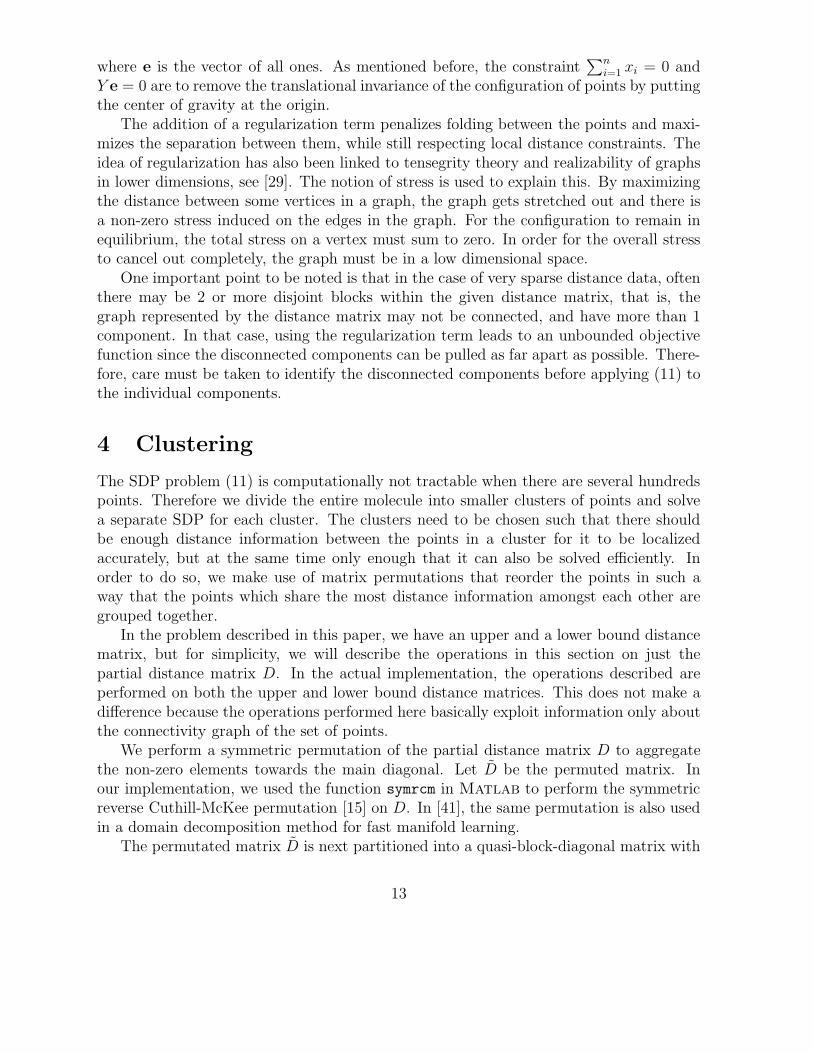
4 Clustering

The SDP problem (11) is computationally not tractable when there are several hundredspoints. Therefore we divide the entire molecule into smaller clusters of points and solvea separate SDP for each cluster. The clusters need to be chosen such that there shouldbe enough distance information between the points in a cluster for it to be localizedaccurately, but at the same time only enough that it can also be solved efficiently. Inorder to do so, we make use of matrix permutations that reorder the points in such away that the points which share the most distance information amongst each other aregrouped together.

In the problem described in this paper, we have an upper and a lower bound distancematrix, but for simplicity, we will describe the operations in this section on just thepartial distance matrix D. In the actual implementation, the operations described areperformed on both the upper and lower bound distance matrices. This does not make adifference because the operations performed here basically exploit information only aboutthe connectivity graph of the set of points.

We perform a symmetric permutation of the partial distance matrix D to aggregatethe non-zero elements towards the main diagonal. Let D be the permuted matrix. Inour implementation, we used the function symrcm in Matlab to perform the symmetricreverse Cuthill-McKee permutation [15] on D. In [41], the same permutation is also usedin a domain decomposition method for fast manifold learning.

The permutated matrix D is next partitioned into a quasi-block-diagonal matrix with

13

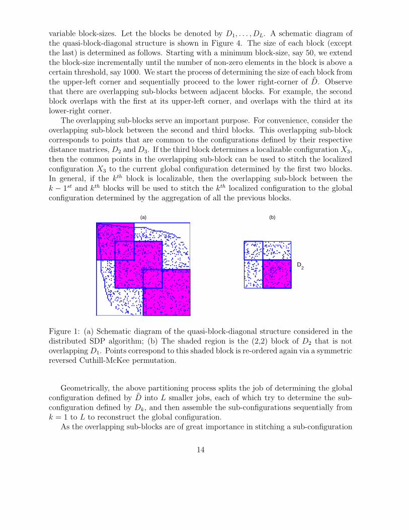
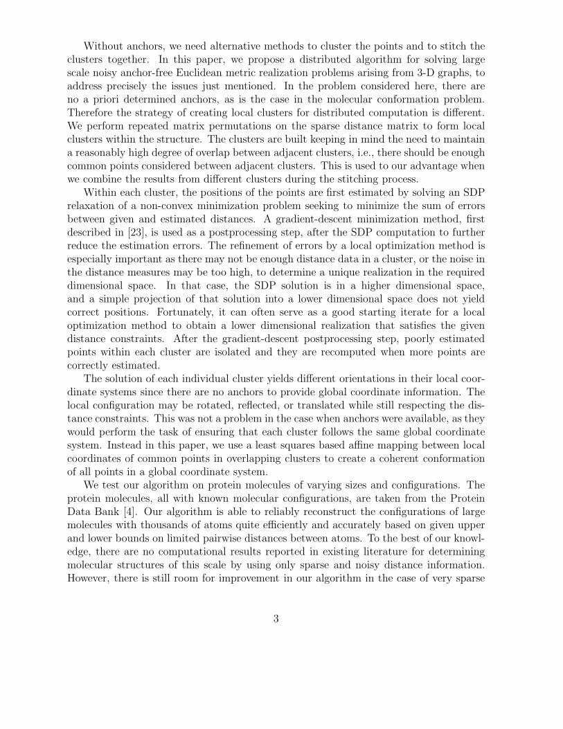
variable block-sizes. Let the blocks be denoted by D1, . . . , DL. A schematic diagram ofthe quasi-block-diagonal structure is shown in Figure 4. The size of each block (exceptthe last) is determined as follows. Starting with a minimum block-size, say 50, we extendthe block-size incrementally until the number of non-zero elements in the block is above acertain threshold, say 1000. We start the process of determining the size of each block fromthe upper-left corner and sequentially proceed to the lower right-corner of D. Observethat there are overlapping sub-blocks between adjacent blocks. For example, the secondblock overlaps with the first at its upper-left corner, and overlaps with the third at itslower-right corner.

The overlapping sub-blocks serve an important purpose. For convenience, consider theoverlapping sub-block between the second and third blocks. This overlapping sub-blockcorresponds to points that are common to the configurations defined by their respectivedistance matrices, D2 and D3. If the third block determines a localizable configuration X3,then the common points in the overlapping sub-block can be used to stitch the localizedconfiguration X3 to the current global configuration determined by the first two blocks.In general, if the kth block is localizable, then the overlapping sub-block between thek − 1st and kth blocks will be used to stitch the kth localized configuration to the globalconfiguration determined by the aggregation of all the previous blocks.

(a) (b)

D2

Figure 1: (a) Schematic diagram of the quasi-block-diagonal structure considered in thedistributed SDP algorithm; (b) The shaded region is the (2,2) block of D2 that is notoverlapping D1. Points correspond to this shaded block is re-ordered again via a symmetricreversed Cuthill-McKee permutation.

Geometrically, the above partitioning process splits the job of determining the globalconfiguration defined by D into L smaller jobs, each of which try to determine the sub-configuration defined by Dk, and then assemble the sub-configurations sequentially fromk = 1 to L to reconstruct the global configuration.

As the overlapping sub-blocks are of great importance in stitching a sub-configuration

14

to the global configuration, it should have as high connectivity as possible. In our im-plementation, we find the following strategy to be reasonably effective. After the blocksD1, . . . , DL are determined, starting with D2, we perform a symmetric reverse Cuthill-McKee permutation to the (2,2) sub-block of D2 that is not overlapping D1, and repeatthe same process sequentially for all subsequent blocks. To avoid introducing excessivenotation, we still use Dk to denote the permuted kth block.

It is also worth noting that in the case of highly noisy or very sparse data, the size ofthe overlapping sub-blocks needs to be set higher for the stitching phase to succeed. Themore common points there are between 2 blocks, the more robust the stitching betweenthem. This is also true as the number of sub-blocks which need to be stitched is large(that is, the number of atoms in the molecules is large). However, increasing the numberof common points also has an impact on the runtime, and therefore we must choose theoverlapping sub-block sizes judiciously. Experiments indicated that a sub-block size of15-20 was sufficient for molecules with less than 3000 atoms but sub-block sizes of 25-30were more suitable for larger molecules.

5 Stitching

After all the individual localization problems corresponding to D1, . . . , DL have beensolved, we have L sub-configurations that need to be assembled together to form theglobal configuration associated with D.

Suppose the current configuration determined by the blocks Di, i = 1, . . . , k − 1 isgiven by the matrix X(k−1) = [U (k−1), V (k−1)]. Suppose also that F (k−1) records theglobal indices of the points that are currently labelled as localized in the current globalconfiguration. Let Xk = [Vk, Wk] be the points in the sub-configuration determined byDk. (For k = 1, Vk is the null matrix. For k = 2, Vk and Wk correspond to the unshadedand shaded sub-blocks of D2 in Figure 1(b), respectively.) Here V (k−1) and Vk denote thepositions of the points corresponding to the overlapping sub-block between Dk−1 and Dk,respectively.

Let Ik be the global indices of the points in Wk. Note that the global indices of theunlocalized points for the blocks D1, . . . , Dk−1 are given by J (k−1) =

⋃k−1i=1 Ii \F (k−1).

We will now concentrate on stitching the sub-configuration Dk with the global indexset Ik. Note that the points in the sub-configuration Dk, which have been obtained bysolving the SDP on Dk, will most likely contain points that have been correctly estimatedand points that have been estimated less accurately. It is essential that we isolate the badlyestimated points, so as to ensure that their errors are not propagated when estimatingsubsequent blocks and that we may recalculate their positions when more points havebeen correctly estimated.

To detect the badly estimated points, we use a combination of 2 error measures. Letxj be the position estimated for point j. Set F ← F (k−1). We use the trace error Tj from

15

Equation (8) and the local error

Ej =

∑i∈Nj

(‖xi − xj‖ − dij)2

|Nj|. (12)

where Nj = {i ∈ F : i < j, Dij 6= 0}. We require max{Tj , Ej} ≤ Tε as a necessarycondition for the point to be correctly estimated.

In the case when we are just provided with upper and lower bounds on distances, weuse the mean distance in the local error measure calculations, i.e.,

dij = (dij + dij)/2. (13)

The use of multiple error measures is crucial, especially in cases when the distanceinformation provided is noisy. In the noise free case, it is much easier to isolate pointswhich are badly estimated using only the trace error Tj . But in the noisy case, thereare no reliable error measures. By using multiple error measures, we hope to identify allthe bad points which might possibly escape detection when only a single error measure isused.

Setting the tolerances Tε for the error is also an important parameter selection issue.For very sparse distance data and highly noisy cases, where even accurately estimatedpoints may have significant error measure values, there is a tradeoff between selecting thetolerance and the number of points that are flagged as badly estimated. If the tolerance istoo tight, we might end up discarding too many points that are actually quite accuratelyestimated.

The design of informative error measures is still an open issue and there is room forimprovement. As our results will show, the stitching phase of the algorithm is one whichis most susceptible to noise and inaccurate estimation, and we need better error measuresto make it more robust.

Now we have two cases to consider in the stitching process.

(i) Suppose that there are enough points in the overlapping sub-blocks Vk and V (k−1)

that are well estimated/localized, then we can stitch the kth sub-configuration di-rectly to the current global configuration X(k−1) by finding the affine mapping thatmatches points in V (k−1) and Vk as closely as possible. Mathematically, we solve thefollowing linear least squares problem:

min{‖B(Vk − α)− (V (k−1) − β)‖F : B ∈ Rd×d

}, (14)

where α and β are the centroids of Vk and V (k−1), respectively. Once an optimal Bis found, set

X = [U (k−1), V (k−1), β + B(Wk − α)], F ← F (k−1)⋃

Ik.

16

We should mention that in the stitching process, it is very important to excludepoints in V (k−1) and Vk that are badly estimated/unlocalized when solving (14) toavoid destroying the current global configuration.

It should also be noted that there may be points in Wk that are incorrectly estimatedin the SDP step. Performing the affine transformation on these points is useless,because they are in the wrong position in the local configuration to begin with. Todeal with these points, we re-estimate the positions using those correctly estimatedpoints as anchors. This procedure is exactly the same as what is described in case(ii).

(ii) If there are not enough common points in the overlapping sub-blocks, then thestitching process described in (a) cannot be carried out successfully. In this case,the solution obtained from the SDP step for Dk is discarded. That is, the positions inWk are discarded and they are to be determined via the current global configurationX(k−1) point-by-point as follows.

Set X ← X(k−1), and F ← F (k−1). Let Tε = 10−4.For j ∈ J (k−1)

⋃Ik,

(1) Formulate the new SDP problem (3) with N = ∅ and M = {(i, j) : i ∈F , Dij 6= 0} where the anchor points are given by {X(:, i) : (i, j) ∈M}.

(2) Let xj and Tj be the newly estimated position and trace error from the previous

step. Compute the local error measure Ej.

If j ∈ J (k−1), set X(:, j) = xj ; else, set X = [X, xj ]. If min{Tj, Ej} ≤ Tε, then

set F ← F ∪ {j}, end.

Notice that in attempting to localize the points corresponding to Wk, we also at-tempt to estimate the positions of those previously unlocalized points, whose indicesare recorded in J (k−1).

Furthermore, we use previously estimated points as anchors to estimate new points.This not only helps in stitching new points into the current global configuration, butalso increases the chances of correcting the positions of previously badly estimatedpoints (since more anchor information is available when more points are correctlyestimated).

17

6 Postprocessing refinement by a gradient descent

method

The positions estimated from the SDP and stitching steps can further be refined byapplying a local optimization method to the following problem:

minX∈Rd×n

{f(X) :=

∑

(i,j)∈N

(‖xi − xj‖ − dij)2 +

∑

(j,k)∈M

(‖xj − ak‖ − hjk)2}. (15)

The method we suggest to improve the current solution is to move every position alongthe negative gradient direction of the function f(X) in (15) to reduce the error functionvalue. Now, we will explain the gradient method in more detail.

Let Nj = {i : (i, j) ∈ N} and Mj = {k : (j, k) ∈ M}. By using the fact that∇x‖x − b‖ = (x − b)/‖x − b‖ if x 6= b, it is easy to show that for the objective functionf(X) in (15), the gradient ∇jf with respect to the position xj is given by:

∇jf(X) = 2∑

i∈Nj

(1− dij

‖xj − xi‖)(xj − xi) + 2

∑

i∈Mj

(1− hjk

‖xj − ak‖)(xj − ak). (16)

Notice that∇jf only involves points that are connected to xj . Thus ∇jf can be computedin a distributed fashion.

The gradient-descent method is a local optimization method that generally does notdeliver the global optimal solution of a non-convex problem, unless a good starting iter-ate is available. The graph realization problem described in this paper is a non-convexoptimization problem. Hence a pure gradient-descent method would not work. However,the SDP estimated solutions are generally close to the global minimum, and so they serveas excellent initial points to start the local optimization.

Different objective functions can also be used in the gradient-descent method, forexample, one could have considered the objective function

∑(i,j)∈N (‖xi − xj‖2 − d2

ij)2 +∑

(j,k)∈M(‖xj − ak‖2 − h2jk)

2 instead of the one in (15). But we have found that thereare no significantly difference in the quality of the estimated positions produced by thegradient method using either objective functions. The one considered in (15) is easilycomputed and is a good indicator of the estimation error. In our implementation, weuse the gradient refinement step quite extensively, both after the SDP step for a singleblock, and also after each stitching phase between 2 blocks. In the single block case, thecalculation does not involve the use of any anchor points, but when used after stitching,we fix the previous correctly estimated points as anchors.

18

7 A distributed SDP algorithm for anchor-free graph

realization

We will now describe the complete distributed algorithm for solving a large scale anchor-free graph realization problem. To facilitate the description of our distributed algorithmfor anchor-free graph realization, we first describe the centralized algorithm for solving(1). It is important to note here that the terms localization and realization are usedinterchangeably.

Centralized graph localization (CGL) algorithm.Input: (D, D,N ; {a1, . . . , am},M).Output: Estimated positions, [x1, . . . , xn] ∈ Rd×n, and corresponding accuracy measures;

trace errors, T1, . . . , Tn and local error measures E1, . . . , En.

1. Formulate the optimization problem (10) and solve the resulting SDP. Let X =[x1, . . . , xn] be the estimated positions obtained from the SDP solution.

2. Perform the gradient-descent algorithm to (15) using the SDP solution as the start-ing iterate to get more refined estimated positions [x1, . . . , xn].

3. For each j = 1, . . . , n, label the point j as localized or unlocalized based on the errormeasures Tj and Ej .

Distributed anchor free graph localization (DAFGL) algorithm.Input : Upper and lower bounds on a subset of the pairwise distances in a molecule.Output : A configuration of all the atoms in the molecule that is closest (in terms of the

RMSD error described in Section 8) to the actual molecule (from which the measurementswere taken).

1. Divide the entire point set into sub-blocks using the clustering algorithm describedin Section 4 on the sparse distance matrices.

2. Apply the CGL algorithm to each sub-block.

3. Stitch the sub-blocks together using the procedure described in Section 5. After eachstitching phase, refine the point positions again using the gradient-descent methoddescribed in Section 6 and update their error measures.

Some remarks are in order for the above algorithm. In Step 3, we can solve eachcluster individually and the computation is highly distributive. In using the centralizedCGL algorithm to solve each cluster, the computational cost is dominated by the solutionof the SDP problem(the SDP cost is in turn determined by the number of given distances).For a graph with n nodes and m given pairwise distances, the computational complexityin solving the SDP is roughly O(m3) + O(n3), provided sparsity in the SDP data is fully

19

exploited. For a graph with 200 nodes and the number of given distances is 10% of thetotal number of pairwise distances, the SDP would roughly have 2000 equality constraintsand matrix variables of dimension 200. Such an SDP can be solved on a Pentium IV 3.0GHz PC with 2GB RAM in about 36 and 93 seconds using the general purpose SDPsoftware SDPT3-3.1 [35] and SeDuMi-1.05 [30], respectively.

The computational efficiency in the CGL algorithm can certainly be improved in var-ious ways. First, the SDP problem need not be solved to high accuracy. It is sufficient tohave a low accuracy SDP solution if it is only used as a starting iterate for the gradient-descent algorithm. There are various highly efficient methods (such as iterative solverbased interior-point methods [31] or the SDPLR method of Burer and Monteiro [10]) toobtain a low accuracy SDP solution. Second, a dedicated solver based on a dual scalingalgorithm can also speed up the SDP computation. Substantial speed up can be expectedif the computation exploits the low rank structure present in the constraint matrices.However, as our focus in this paper is not on improving the computational efficiency ofthe CGL algorithm, we shall not discuss this issue further. In the numerical experimentsconducted in Section 8, we use the softwares SDPT3-3.1 and SeDuMi to solve the SDP inthe CGL algorithm. An alternative is to use the software DSDP5.6 [3], which is expectedto be more efficient than SDPT3-3.1 or SeDuMi.

The stitching process in Step 4 is sequential in nature. But this does not imply thatthe distributed DAFGL algorithm is redundant and that the centralized CGL algorithmis sufficient for computational purpose. For a graph with 10000 nodes and the numberof given distances is 1% of the total number of all pairwise distances, the SDP problemthat needs to be solved by the CGL algorithm would have 500000 constraints and matrixvariables of dimension 10000. Such a large scale SDP is well beyond the range that canbe solved routinely on a standard workstation available today. By considering smallerblocks, the distributed algorithm does not suffer from the limitation faced by the CGLalgorithm.

If there are multiple computer processors available, say p of them, the distributedalgorithm can also take advantage of the extra computing power. The strategy is todivide the graph into p large blocks using Step 2 of the algorithm and apply the DAFGLalgorithm to localize one large block on each processor.

We end this section with two observations on the DAFGL algorithm. First, we ob-served that usually the outlying points which have low connectivity are not well estimatedin the initial stages of the method. As the number of well estimated points grows gradually,more and more of these “loose” points are estimated by the gradient-descent algorithm.As the molecules get larger, the frequency of having non-localizable sub-configurationsin Step 4 also increases. Thus the point-by-point stitching procedure of the algorithmdescribed in Section 5 gets visited more and more often.

Second, for large molecules, the sizes of the overlapping-blocks need to be larger for thestitching algorithm in Section 5 to be robust (more common points generally lead to moreaccuracy in stitching). But to accommodate larger overlapping-blocks, each subgraph

20

in the DAFGL algorithm will correspondingly be larger, and that in turns increases theproblem size of the SDP relaxation. In our implementation, we apply the idea of droppingredundant constraints to reduce the computational effort in selecting large sub-block sizesof 100-150. This strategy works because many of the distance constraints are for some ofthe densest parts of the sub-block, and the points in these dense sections can actually beestimated quite well with only a fraction of those distance constraints. Therefore in theSDP step, we limit the number of distance constraints for each point to below 6. If thereare more distance constraints, they are not included in the SDP step. This allows us tochoose large overlapping-block sizes while the corresponding SDPs for larger clusters canbe solved without too much additional computational effort.

8 Computational results

To evaluate our DAFGL algorithm, numerical experiments were performed on proteinmolecules with the number of atoms in each molecule ranging from a few hundreds to afew thousands. We conducted our numerical experiments in Matlab on a single PentiumIV 3.0 GHz PC with 2GB of RAM. The known 3D coordinates of the atoms were takenfrom the Protein Data Bank (PDB) [4]. These were used to generate the true distancesbetween the atoms. Our goal in the experiments is to reconstruct as closely as possiblethe known molecular configuration for each molecule, using only distance informationgenerated from a sparse subset of all the pairwise distances. This information was in theform of upper and lower bounds on the actual pairwise distances.

For each molecule, we generated the partial distance matrix as follows. If the distancebetween 2 atoms was less than a given cutoff radius R, the distance is kept; otherwise,no distance information is known about the pair. The cutoff radius R is chosen to be6A (1A = 10−8cm), which is roughly the maximum distance that NMR techniques canmeasure between two atoms. Therefore, in this case, N = {(i, j) : ‖xi − xj‖ ≤ 6A}.

We then perturb the distances to generate upper and lower bounds on the givendistances in the following manner. Assume that dij is the true distance between atom iand atom j, we set

dij = dij(1 + |εij|)dij = dij max(0, 1− |εij |),

where εij, εij ∼ N (0, σ2ij)

By varying σij (which we keep as the same for all pairwise distances), we control thenoise in the data. This is a multiplicative noise model, where a higher distance valuemeans more uncertainty in its measurement. For all future reference, we will refer to σij

in percentage values. For example, σij = 0.1 will be referred to as 10% noise on the upperand lower bounds.

Typically, not all the distances below 6A are known from NMR experiments. There-fore, we will also present results for the DAFGL algorithm when only a fraction of all the

21

distances below 6A are chosen randomly and used in the calculation.Let Q be the set of orthogonal matrices in Rd×d (d = 3). We measure the accuracy

performance of our algorithm by the following criteria:

RMSD =1√n

min{‖Xtrue −QX − h‖F |Q ∈ Q, h ∈ Rd

}(17)

LDME =( 1

|N |∑

(i,j)∈N

(‖xi − xj‖ − dij

)2)1/2

. (18)

The first criterion RMSD (root mean square deviation) requires the knowledge of thetrue configuration, whereas the second does not. Thus the second criterion LDME (localdistance matrix error) is more practical but it is also less reliable in evaluating the trueaccuracy of the constructed configuration. The practically useful measure LDME giveslower values than the RMSD, and as the noise increases, it is not a very reliable measure.

When 90% of the distances (below 6A) or higher were given, and were not corruptedby noise, the molecules considered here were estimated very precisely with RMSD =10−4−10−6A. This goes to show that the algorithm performs remarkably well when thereis enough exact distance data. In this regard, our algorithm is competitive compared to thegeometric build-up algorithm in [38] which is designed specifically for graph localizationwith exact distance data. With exact distance data, we have solved molecules that aremuch larger and with much sparser distance data than those considered in [38].

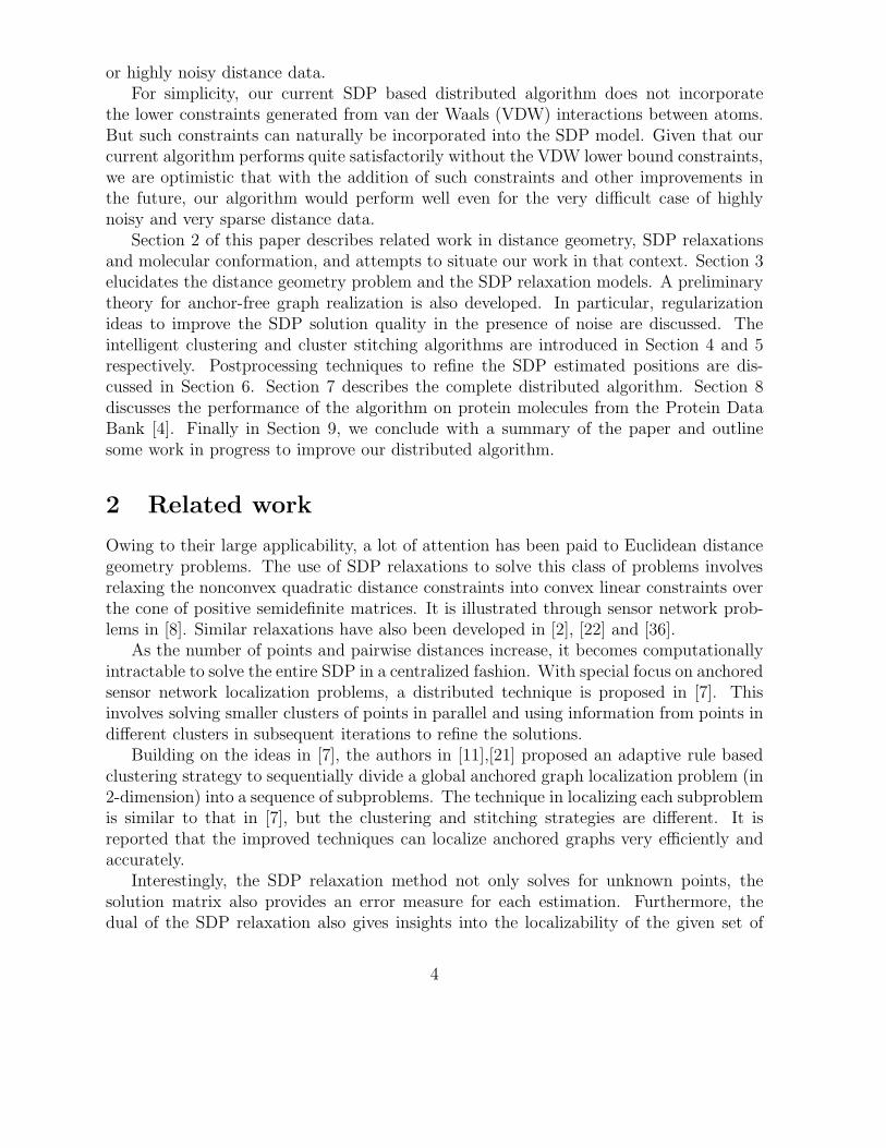
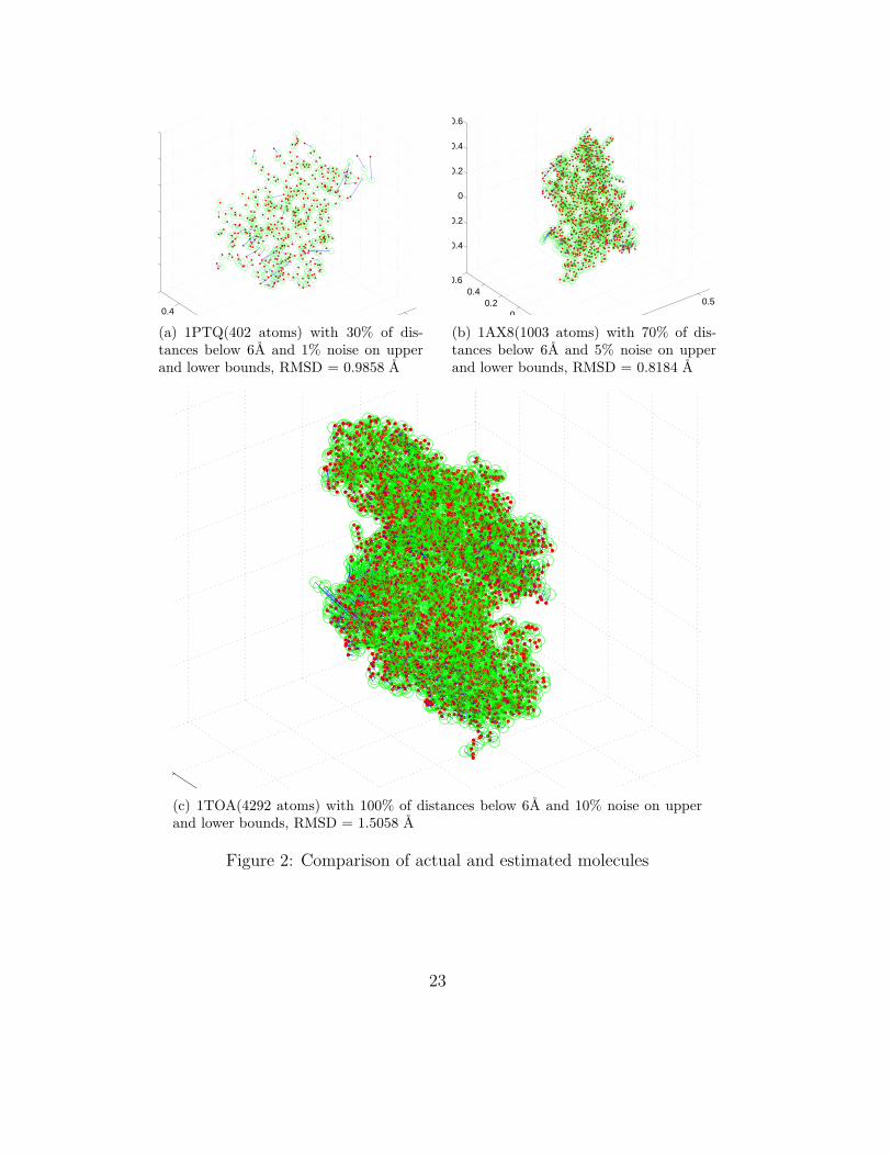
However, our focus in this paper is more on molecular conformation with noisy andsparse distance data. We will only present results for such cases. In Figure 2, the originaltrue and the estimated atom positions are plotted for some of the molecules, with vary-ing amounts of distance data and noise. The open green circles correspond to the truepositions and solid red dots to their estimated positions from our computation. The erroroffset between the true and estimated positions for an individual atom is depicted by asolid blue line. The solid lines, however, are not visible for most of the atoms in the plotsbecause we are able to estimate the positions very accurately.

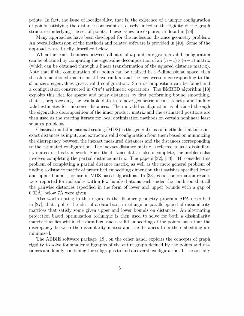
The plots show that even for very sparse data (as in the case of 1PTQ), the estimationfor most of the atoms is accurate. The atoms that are badly estimated are the ones thathave too little distance information for them to be localized. The algorithm also performswell for very noisy data, and for large molecules, as demonstrated for 1AX8 and 1TOA.The largest molecule we tried the algorithm on is 1I7W, with 8629 atoms. Figure 3 showsthat even when the distance data is highly noisy (10 % error on upper and lower bounds),the estimation is close to the original with an RMSD error = 1.3842 A.

However, despite using more common points for stitching, the DAFGL algorithmcan sometimes generate estimations with high RMSD error for very large molecules dueto a combination of irregular geometry, very sparse distance data and noisy distances.Ultimately, the problem boils down to being able to correctly identify when a point hasbeen badly estimated. Our measures using trace error (8) and local error (12) are ableto isolate the majority of the points that are badly estimated, but do not always succeed

22

0.50.4

0.6

−0.4

−0.2

0

0.2

0.4

0.6

(a) 1PTQ(402 atoms) with 30% of dis-tances below 6A and 1% noise on upperand lower bounds, RMSD = 0.9858 A

0.50

0.20.4

0.6

−0.4

−0.2

0

0.2

0.4

0.6

(b) 1AX8(1003 atoms) with 70% of dis-tances below 6A and 5% noise on upperand lower bounds, RMSD = 0.8184 A

(c) 1TOA(4292 atoms) with 100% of distances below 6A and 10% noise on upperand lower bounds, RMSD = 1.5058 A

Figure 2: Comparison of actual and estimated molecules

23

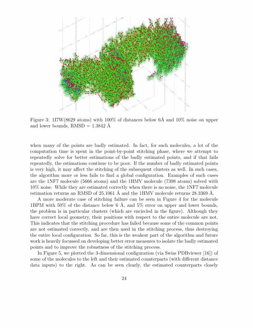
Figure 3: 1I7W(8629 atoms) with 100% of distances below 6A and 10% noise on upperand lower bounds, RMSD = 1.3842 A

when many of the points are badly estimated. In fact, for such molecules, a lot of thecomputation time is spent in the point-by-point stitching phase, where we attempt torepeatedly solve for better estimations of the badly estimated points, and if that failsrepeatedly, the estimations continue to be poor. If the number of badly estimated pointsis very high, it may affect the stitching of the subsequent clusters as well. In such cases,the algorithm more or less fails to find a global configuration. Examples of such casesare the 1NF7 molecule (5666 atoms) and the 1HMV molecule (7398 atoms) solved with10% noise. While they are estimated correctly when there is no noise, the 1NF7 moleculeestimation returns an RMSD of 25.1061 A and the 1HMV molecule returns 28.3369 A.

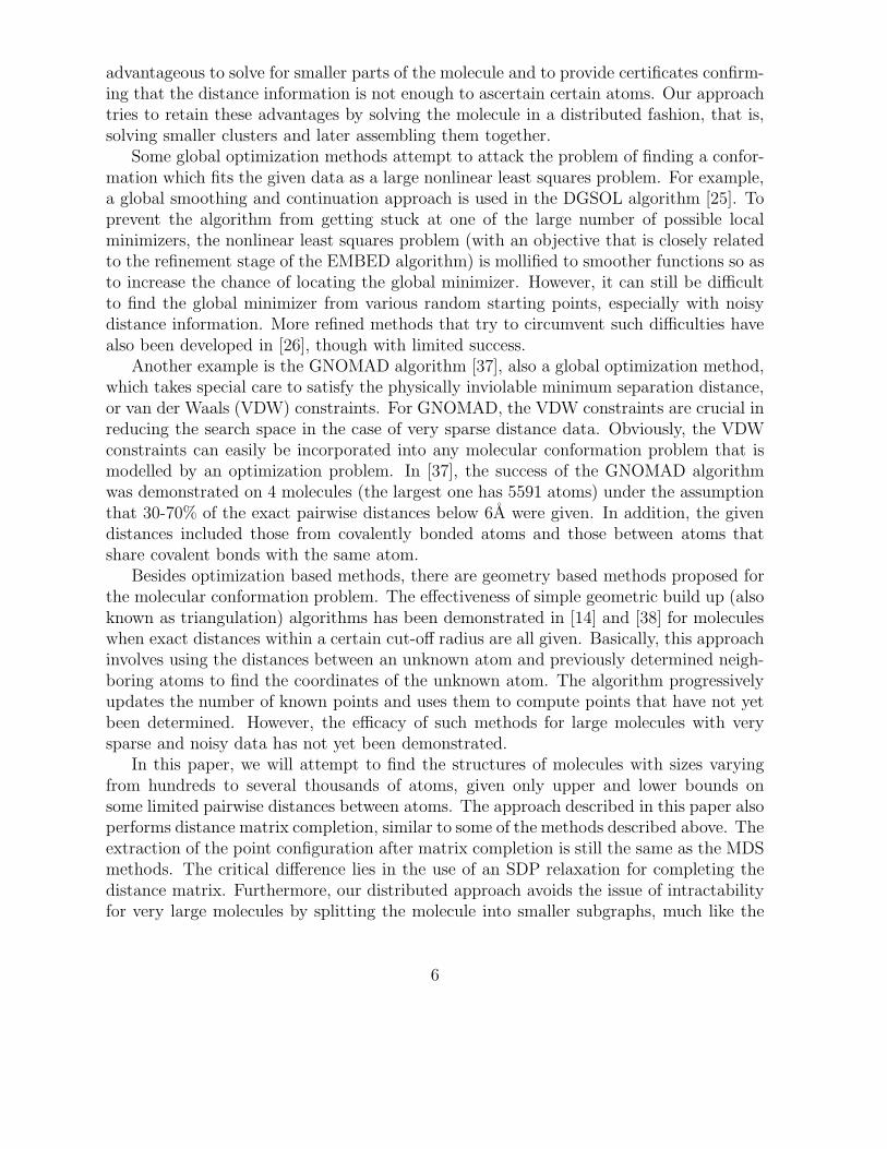
A more moderate case of stitching failure can be seen in Figure 4 for the molecule1BPM with 50% of the distance below 6 A, and 5% error on upper and lower bounds,the problem is in particular clusters (which are encircled in the figure). Although theyhave correct local geometry, their positions with respect to the entire molecule are not.This indicates that the stitching procedure has failed because some of the common pointsare not estimated correctly, and are then used in the stitching process, thus destroyingthe entire local configuration. So far, this is the weakest part of the algorithm and futurework is heavily focussed on developing better error measures to isolate the badly estimatedpoints and to improve the robustness of the stitching process.

In Figure 5, we plotted the 3-dimensional configuration (via Swiss PDBviewer [16]) ofsome of the molecules to the left and their estimated counterparts (with different distancedata inputs) to the right. As can be seen clearly, the estimated counterparts closely

24

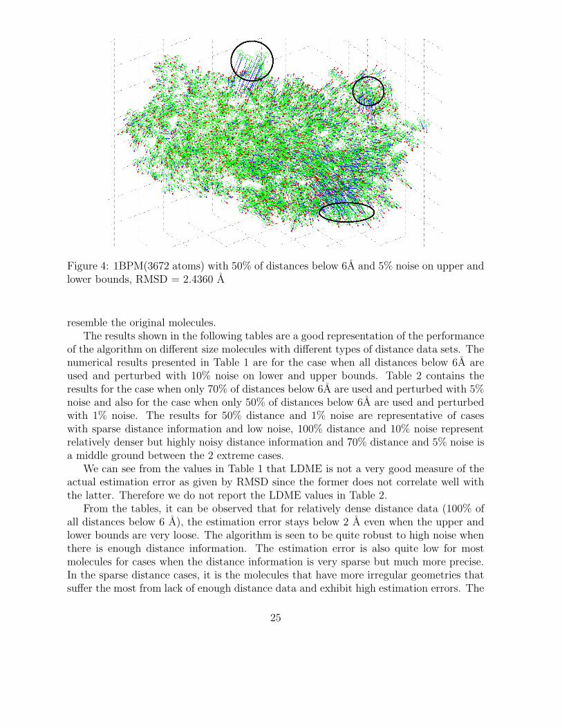
Figure 4: 1BPM(3672 atoms) with 50% of distances below 6A and 5% noise on upper andlower bounds, RMSD = 2.4360 A

resemble the original molecules.The results shown in the following tables are a good representation of the performance

of the algorithm on different size molecules with different types of distance data sets. Thenumerical results presented in Table 1 are for the case when all distances below 6A areused and perturbed with 10% noise on lower and upper bounds. Table 2 contains theresults for the case when only 70% of distances below 6A are used and perturbed with 5%noise and also for the case when only 50% of distances below 6A are used and perturbedwith 1% noise. The results for 50% distance and 1% noise are representative of caseswith sparse distance information and low noise, 100% distance and 10% noise representrelatively denser but highly noisy distance information and 70% distance and 5% noise isa middle ground between the 2 extreme cases.

We can see from the values in Table 1 that LDME is not a very good measure of theactual estimation error as given by RMSD since the former does not correlate well withthe latter. Therefore we do not report the LDME values in Table 2.

From the tables, it can be observed that for relatively dense distance data (100% ofall distances below 6 A), the estimation error stays below 2 A even when the upper andlower bounds are very loose. The algorithm is seen to be quite robust to high noise whenthere is enough distance information. The estimation error is also quite low for mostmolecules for cases when the distance information is very sparse but much more precise.In the sparse distance cases, it is the molecules that have more irregular geometries thatsuffer the most from lack of enough distance data and exhibit high estimation errors. The

25

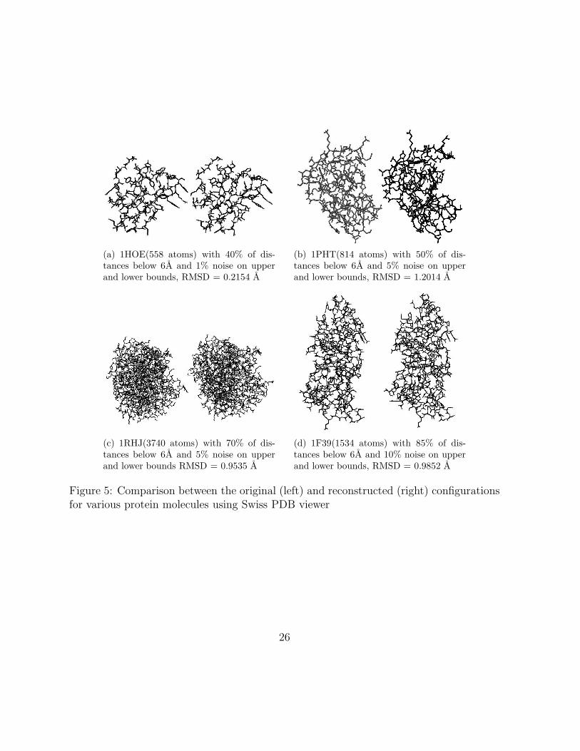
(a) 1HOE(558 atoms) with 40% of dis-tances below 6A and 1% noise on upperand lower bounds, RMSD = 0.2154 A

(b) 1PHT(814 atoms) with 50% of dis-tances below 6A and 5% noise on upperand lower bounds, RMSD = 1.2014 A

(c) 1RHJ(3740 atoms) with 70% of dis-tances below 6A and 5% noise on upperand lower bounds RMSD = 0.9535 A

(d) 1F39(1534 atoms) with 85% of dis-tances below 6A and 10% noise on upperand lower bounds, RMSD = 0.9852 A

Figure 5: Comparison between the original (left) and reconstructed (right) configurationsfor various protein molecules using Swiss PDB viewer

26

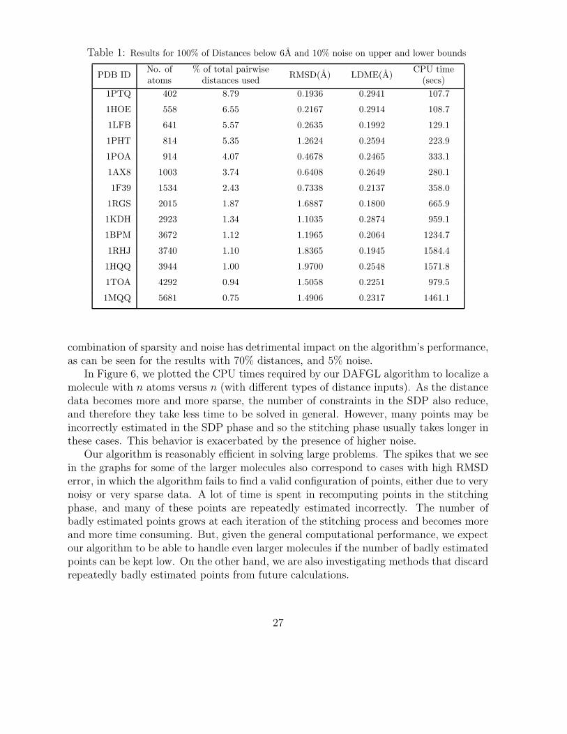
Table 1: Results for 100% of Distances below 6A and 10% noise on upper and lower bounds

PDB IDNo. ofatoms

% of total pairwisedistances used

RMSD(A) LDME(A)CPU time

(secs)

1PTQ 402 8.79 0.1936 0.2941 107.7

1HOE 558 6.55 0.2167 0.2914 108.7

1LFB 641 5.57 0.2635 0.1992 129.1

1PHT 814 5.35 1.2624 0.2594 223.9

1POA 914 4.07 0.4678 0.2465 333.1

1AX8 1003 3.74 0.6408 0.2649 280.1

1F39 1534 2.43 0.7338 0.2137 358.0

1RGS 2015 1.87 1.6887 0.1800 665.9

1KDH 2923 1.34 1.1035 0.2874 959.1

1BPM 3672 1.12 1.1965 0.2064 1234.7

1RHJ 3740 1.10 1.8365 0.1945 1584.4

1HQQ 3944 1.00 1.9700 0.2548 1571.8

1TOA 4292 0.94 1.5058 0.2251 979.5

1MQQ 5681 0.75 1.4906 0.2317 1461.1

combination of sparsity and noise has detrimental impact on the algorithm’s performance,as can be seen for the results with 70% distances, and 5% noise.

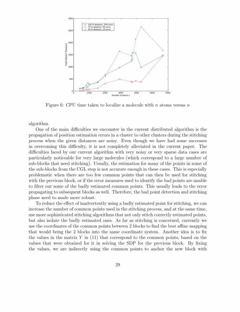
In Figure 6, we plotted the CPU times required by our DAFGL algorithm to localize amolecule with n atoms versus n (with different types of distance inputs). As the distancedata becomes more and more sparse, the number of constraints in the SDP also reduce,and therefore they take less time to be solved in general. However, many points may beincorrectly estimated in the SDP phase and so the stitching phase usually takes longer inthese cases. This behavior is exacerbated by the presence of higher noise.

Our algorithm is reasonably efficient in solving large problems. The spikes that we seein the graphs for some of the larger molecules also correspond to cases with high RMSDerror, in which the algorithm fails to find a valid configuration of points, either due to verynoisy or very sparse data. A lot of time is spent in recomputing points in the stitchingphase, and many of these points are repeatedly estimated incorrectly. The number ofbadly estimated points grows at each iteration of the stitching process and becomes moreand more time consuming. But, given the general computational performance, we expectour algorithm to be able to handle even larger molecules if the number of badly estimatedpoints can be kept low. On the other hand, we are also investigating methods that discardrepeatedly badly estimated points from future calculations.

27

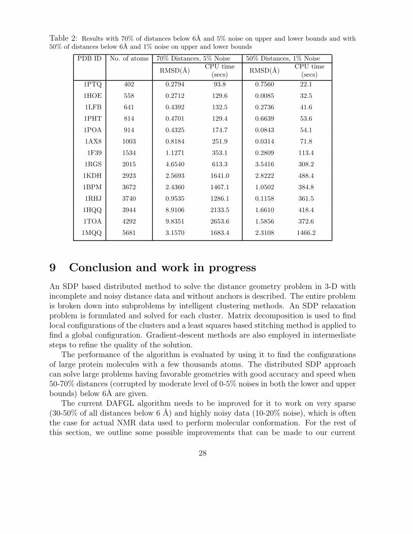
Table 2: Results with 70% of distances below 6A and 5% noise on upper and lower bounds and with50% of distances below 6A and 1% noise on upper and lower bounds

PDB ID No. of atoms 70% Distances, 5% Noise 50% Distances, 1% Noise

RMSD(A)CPU time

(secs)RMSD(A)

CPU time(secs)

1PTQ 402 0.2794 93.8 0.7560 22.1

1HOE 558 0.2712 129.6 0.0085 32.5

1LFB 641 0.4392 132.5 0.2736 41.6

1PHT 814 0.4701 129.4 0.6639 53.6

1POA 914 0.4325 174.7 0.0843 54.1

1AX8 1003 0.8184 251.9 0.0314 71.8

1F39 1534 1.1271 353.1 0.2809 113.4

1RGS 2015 4.6540 613.3 3.5416 308.2

1KDH 2923 2.5693 1641.0 2.8222 488.4

1BPM 3672 2.4360 1467.1 1.0502 384.8

1RHJ 3740 0.9535 1286.1 0.1158 361.5

1HQQ 3944 8.9106 2133.5 1.6610 418.4

1TOA 4292 9.8351 2653.6 1.5856 372.6

1MQQ 5681 3.1570 1683.4 2.3108 1466.2

9 Conclusion and work in progress

An SDP based distributed method to solve the distance geometry problem in 3-D withincomplete and noisy distance data and without anchors is described. The entire problemis broken down into subproblems by intelligent clustering methods. An SDP relaxationproblem is formulated and solved for each cluster. Matrix decomposition is used to findlocal configurations of the clusters and a least squares based stitching method is applied tofind a global configuration. Gradient-descent methods are also employed in intermediatesteps to refine the quality of the solution.

The performance of the algorithm is evaluated by using it to find the configurationsof large protein molecules with a few thousands atoms. The distributed SDP approachcan solve large problems having favorable geometries with good accuracy and speed when50-70% distances (corrupted by moderate level of 0-5% noises in both the lower and upperbounds) below 6A are given.

The current DAFGL algorithm needs to be improved for it to work on very sparse(30-50% of all distances below 6 A) and highly noisy data (10-20% noise), which is oftenthe case for actual NMR data used to perform molecular conformation. For the rest ofthis section, we outline some possible improvements that can be made to our current

28

0 1000 2000 3000 4000 5000 60000

500

1000

1500

2000

2500

3000

Number of atoms n

Tot

al S

olut

ion

Tim

e(se

c)

100 % distance, 10% error70 % distance, 5% error50 % distance, 1% error

Figure 6: CPU time taken to localize a molecule with n atoms versus n

algorithm.One of the main difficulties we encounter in the current distributed algorithm is the

propagation of position estimation errors in a cluster to other clusters during the stitchingprocess when the given distances are noisy. Even though we have had some successesin overcoming this difficulty, it is not completely alleviated in the current paper. Thedifficulties faced by our current algorithm with very noisy or very sparse data cases areparticularly noticeable for very large molecules (which correspond to a large number ofsub-blocks that need stitching). Usually, the estimation for many of the points in some ofthe sub-blocks from the CGL step is not accurate enough in these cases. This is especiallyproblematic when there are too few common points that can then be used for stitchingwith the previous block, or if the error measures used to identify the bad points are unableto filter out some of the badly estimated common points. This usually leads to the errorpropagating to subsequent blocks as well. Therefore, the bad point detection and stitchingphase need to made more robust.

To reduce the effect of inadvertently using a badly estimated point for stitching, we canincrease the number of common points used in the stitching process, and at the same time,use more sophisticated stitching algorithms that not only stitch correctly estimated points,but also isolate the badly estimated ones. As far as stitching is concerned, currently weuse the coordinates of the common points between 2 blocks to find the best affine mappingthat would bring the 2 blocks into the same coordinate system. Another idea is to fixthe values in the matrix Y in (11) that correspond to the common points, based on thevalues that were obtained for it in solving the SDP for the previous block. By fixingthe values, we are indirectly using the common points to anchor the new block with

29

the previous one. The dual of the SDP relaxation also merits further investigation, forpossible improvements in the computational effort required and for more robust stitchingresults.

With regard to error measures, it would be useful to study if the local error measure(12) can be made more sophisticated by including a larger set of points to check its dis-tances with, as opposed to just its immediate neighborhood. In some cases, the distancesare satisfied within local clusters, but the entire cluster itself is badly estimated (and thelocal error measure fails to filter out many of the badly estimated points in this scenario).Also, we need to investigate the careful selection of the tolerance Tε in deciding whichpoints have been estimated correctly and can be used for stitching.

As has been noted before, our current algorithm does not use the VDW minimumseparation distance constraints of the form ‖xi−xj‖ ≥ Lij described in [27] and [37]. TheVDW constraints played an essential role in those previous work in reducing the searchspace of valid configurations, especially in the case of sparse data where there are manypossible configurations fitting the sparse distance constraints. As mentioned in Section3, VDW lower bound constraints can be added to the SDP model, but we would needto keep track of the type of atom to which each point corresponds. However, one mustbe mindful that the VDW constraints should only be added when necessary so as not tointroduce too many redundant constraints. If the VDW constraints between all pairs ofatoms are added to the SDP model, then the number of lower bound constraints is of theorder n2, where n is the number of points. Thus even if n is below 100, the total numberof constraints could be in the range of thousands. However, many of the VDW constraintsare for two very remote points, and they are often inactive or redundant at the optimalsolution. Therefore, we can adopt an iterative active constraint generation approach. Wefirst solve the SDP problem by completely ignoring the VDW lower bound constraintsto obtain a solution. Then we verify the VDW lower bound constraints at the currentsolution for all the points and add the violated ones into the model. We can repeat thisprocess until all the VDW constraints are satisfied. Typically, we would expect only O(n)VDW constraints to be active at the final solution.

We are optimistic that by combining the ideas presented in previous work on molecularconformation (especially incorporating domain knowledge such as the minimum separationdistances derived from VDW interactions) with the distributed SDP based algorithmin this paper, the improved distributed algorithm would likely be able to calculate theconformation of large protein molecules with satisfactory accuracy and efficiency in thefuture. Based on the performance of the current DAFGL algorithm, and the promisingimprovements to the algorithm we have outlined, a realistic target for us to set in thefuture is to correctly calculate the conformation of a large molecule (with 5000 atoms ormore) given only about 50% of all pairwise distances below 6A, and corrupted by 10-20%noise.

30

Acknowledgements

We would like to thank the anonymous referees for their insightful comments and sugges-tions that lead to a major revision of the paper.

References

[1] S. Al-Homidan and H. Wolkowicz. Approximate and exact completion problems foreuclidean distane matrices using semidefinite programming. Linear Algebra Appl.,406:109–141, 2005.

[2] A. Y. Alfakih, A. Khandani, and H. Wolkowicz. Solving euclidean distance matrixcompletion problems via semidefinite programming. Comput. Optim. Appl., 12(1-3):13–30, 1999.

[3] S. J. Benson, Y. Ye, and X. Zhang. Solving large-scale sparse semidefinite programsfor combinatorial optimization. SIAM Journal on Optimization, 10(2):443–461, 2000.

[4] H. M. Berman, J. Westbrook, Z. Feng, G. Gilliland, T. N. Bhat, H. Weissig, I. N.Shindyalov, and P. E. Bourne. The Protein data bank. Nucleic Acids Research,28:235–242, 2000.

[5] P. Biswas, T.-C. Liang, K.-C. Toh, T.-C. Wang, and Y. Ye. Semidefinite programmingapproaches for sensor network localization with noisy distance measurements. IEEETransactions on Automation Science and Engineeering, Special Issue on DistributedSensing, 3(4):360–371, October 2006.

[6] P. Biswas, T.-C. Liang, T.-C. Wang, and Y. Ye. Semidefinite programming basedalgorithms for sensor network localization. ACM Transactions on Sensor Networks,2(2):188–220, 2006.

[7] P. Biswas and Y. Ye. A distributed method for solving semidefinite programs aris-ing from ad hoc wireless sensor network localization. Technical report, Dept ofManagement Science and Engineering, Stanford University, to appear in MultiscaleOptimization Methods and Applications, October 2003.

[8] P. Biswas and Y. Ye. Semidefinite programming for ad hoc wireless sensor networklocalization. In Proceedings of the third international symposium on Informationprocessing in sensor networks, pages 46–54. ACM Press, 2004.

[9] S. Boyd, L. El Ghaoui, E. Feron, and V. Balakrishnan. Linear Matrix Inequalities inSystem and Control Theory. SIAM., 1994.

31

[10] S. Burer and R. D. C. Monteiro. A nonlinear programming algorithm for solv-ing semidefinite programs via low-rank factorization. Mathematical Programming,95(2):329–357, 2003.

[11] M. Carter, H. H. Jin, M. A. Saunders, and Y. Ye. Spaseloc: An adaptable subproblemalgorithm for scalable wireless network localization. Submitted to the SIAM J. onOptimization, January 2005.

[12] B. Chazelle, C. Kingsford, and M. Singh. The side-chain positioning problem: asemidefinite programming formulation with new rounding schemes. In PCK50: Pro-ceedings of the Paris C. Kanellakis memorial workshop on Principles of computing& knowledge, pages 86–94. ACM Press, 2003.

[13] G. Crippen and T. Havel. Distance geometry and molecular conformation. Wiley,1988.

[14] Q. Dong and Z. Wu. A geometric build-up algorithm for solving the moleculardistance geometry problem with sparse distance data. J. of Global Optimization,26(3):321–333, 2003.

[15] A. George and J.W. Liu. Computer Solution of Large Sparse Positive Definite. Pren-tice Hall Professional Technical Reference, 1981.

[16] N. Guex and M. C. Peitsch. Swiss-model and the Swiss-Pdbviewer: An environmentfor comparative protein modeling. Electrophoresis, 18:2714–2723, 1997.

[17] O. Guler and Y. Ye. Convergence behavior of interior point algorithms. MathematicalProgramming, 60:215–228, 1993.

[18] T. F. Havel and K. Wthrich. An evaluation of the combined use of nuclear magneticresonance and distance geometry for the determination of protein conformation insolution. Journal of Molelcular Biolology, 182:281–294, 1985.

[19] B. A. Hendrickson. The molecular problem: Determining Conformation from pairwisedistances. PhD thesis, Cornell University, 1991.

[20] G. Iyengar, D. Phillips, and C. Stein. Approximation algorithms for semidefinitepacking problems with applications to maxcut and graph coloring. In Eleventh Con-ference on Integer Programming and Combinatorial Optimization, Berlin, 2005.

[21] H. H. Jin. Scalable Sensor Localization Algorithms for Wireless Sensor Networks.PhD thesis, Department of Mechanical and Industrial Engineering, University ofToronto, 2005.

[22] M. Laurent. Matrix completion problems. The Encyclopedia of Optimization, 3:221–229, 2001.

32

[23] T.-C. Liang, T.-C. Wang, and Y. Ye. A gradient search method to round the semidef-inite programming relaxation solution for ad hoc wireless sensor network localization.Technical report, Dept of Management Science and Engineering, Stanford University,August 2004.

[24] N. Linial, E. London, and Y. Rabinovich. The geometry of graphs and some of itsalgorithmic applications. Combinatorica, 15:215–245, 1995.

[25] J. More and Z. Wu. Global continuation for distance geometry problems. SIAMJournal on Optimization., 7:814–836, 1997.

[26] Jorge J. More and Z. Wu. ε-optimal solutions to distance geometry problems viaglobal continuation. Preprint MCS–P520–0595, Mathematics and Computer ScienceDivision, Argonne National Laboratory, Argonne, Ill., May 1994.

[27] R. Reams, G. Chatham, W. K. Glunt, D. McDonald, and T. L. Hayden. Determiningprotein structure using the distance geometry program apa. Computers & Chemistry,23(2):153–163, 1999.

[28] A. M.-C. So and Y. Ye. Theory of semidefinite programming relaxation for sensornetwork localization. Technical report, Dept of Management Science and Engineering,Stanford University, in SODA’5 and to appear in Mathematical Programming, April2004.

[29] A. M.-C. So and Y. Ye. A semidefinite programming approach to tensegrity the-ory and realizability of graphs. Technical report, Dept of Management Science andEngineering, Stanford University, to appear in SODA’06, July 2005.

[30] J. F. Sturm. Using SeDuMi 1.02, a MATLAB toolbox for optimization over symmet-ric cones. Optimization Methods and Software, 11 & 12:625–633, 1999.

[31] K.-C. Toh. Solving large scale semidefinite programs via an iterative solver on theaugmented systems. SIAM J. on Optimization, 14(3):670–698, 2003.

[32] M. W. Trosset. Applications of multidimensional scaling to molecular conformation.Computing Science and Statistics, 29:148–152, 1998.

[33] M. W. Trosset. Distance matrix completion by numerical optimization. Comput.Optim. Appl., 17(1):11–22, 2000.

[34] M. W. Trosset. Extensions of classical multidimensional scaling via variable reduc-tion. Computational Statistics, 17(2):147–162, 2002.

[35] R. H. Tutuncu, K. C. Toh, and M. J. Todd. Solving semidefinite-quadratic-linearprograms using SDPT3. Mathematical Programming, Series B, 95:189–217, 2003.

33

[36] K. Q. Weinberger, F. Sha, and L. K. Saul. Learning a kernel matrix for nonlineardimensionality reduction. In ICML ’04: Proceedings of the twenty-first internationalconference on Machine learning, page 106, New York, NY, USA, 2004. ACM Press.

[37] G. A. Williams, J. M. Dugan, and R. B. Altman. Constrained global optimizationfor estimating molecular structure from atomic distances. Journal of ComputationalBiology, 8(5):523–547, 2001.

[38] D. Wu and Z. Wu. An updated geometric build-up algorithm for molecular distancegeometry problems with sparse distance data., submitted 2003.

[39] Y. Ye and J. Zhang. An improved algorithm for approximating the radii of pointsets. In RANDOM-APPROX, pages 178–187, 2003.

[40] J.-M. Yoon, Y. Gad, and Z. Wu. Mathematical modeling of protein structure us-ing distance geometry. Technical report, Department of Computational & AppliedMathematics, Rice University, 2000.

[41] Z. Zhang and H. Zha. Principal manifolds and nonlinear dimension reduction vialocal tangent space alignment. SIAM Journal of Scientific Computing, 26:313–338,2004.

34