Embed Size (px)
Citation preview
A Distributed Algorithm for the Dead End Problem of Location Based
Routing in Sensor Networks
Le Zou, Mi Lu, Zixiang Xiong,Department of Electrical Engineering, Texas A&M University
IEEE Transactions ,Vehicular Technology 2005

Outline
• Introduction• Network Model• The PAGER (partial-partition avoiding
geographic routing) Algorithm• Simulation• Conclusions

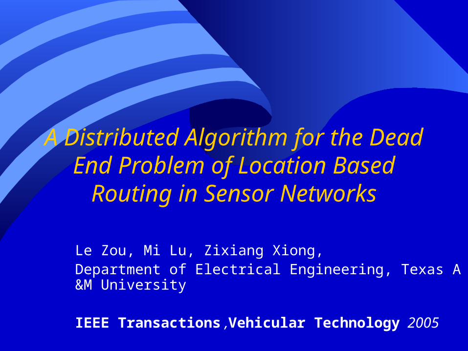
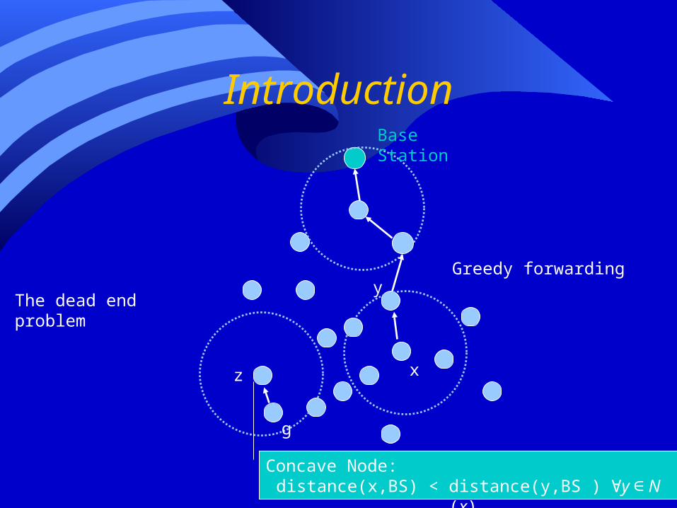
Introduction
Base Station
Sensor nodes
Sensor nodes forward data packets to BS in a multihop manner
IntroductionBase Station
The dead end problem
x
yGreedy forwarding
z
g
Concave Node:distance(x,BS) < distance(y,BS ) y N∀ ∈ (x),

Introduction
Sink Destination
• GPSR (RHR)
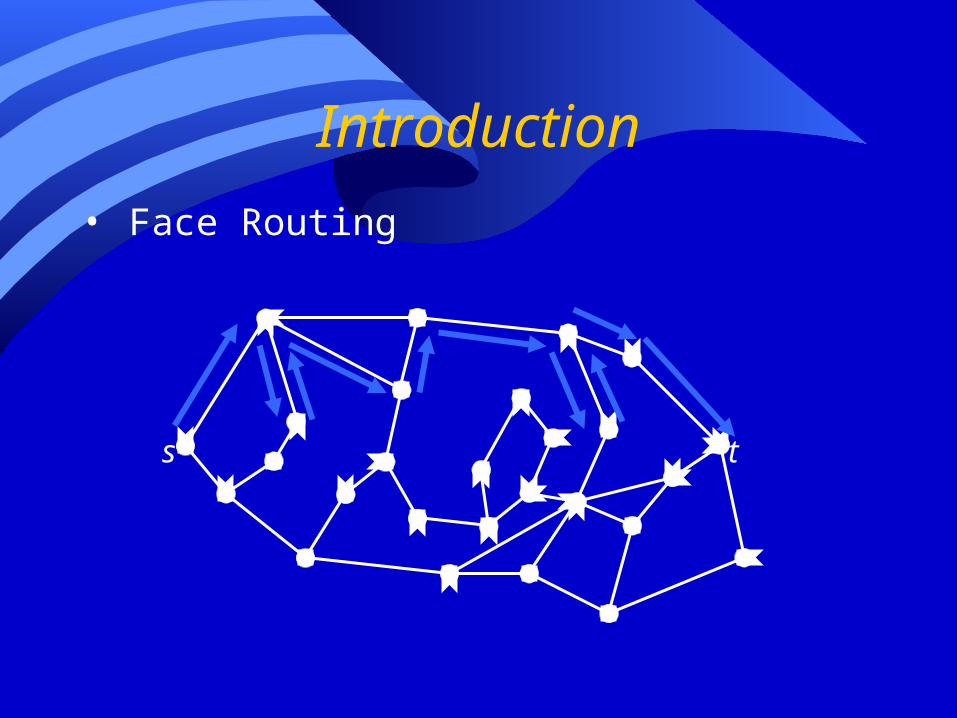
Introduction
s t
• Face Routing
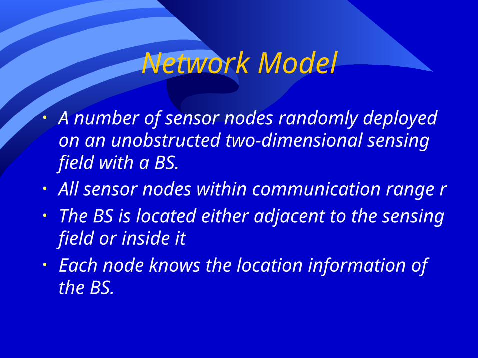
Network Model
• A number of sensor nodes randomly deployed on an unobstructed two-dimensional sensing field with a BS.
• All sensor nodes within communication range r• The BS is located either adjacent to the
sensing field or inside it• Each node knows the location information of
the BS.

The PAGER Algorithm
• The Shadow Spread Phase• Divides a connected graph into subgraphs orig
inated from concave nodes
• The Cost Spread Phase• Establishes paths on a given subgraph obtain
ed in the first phase
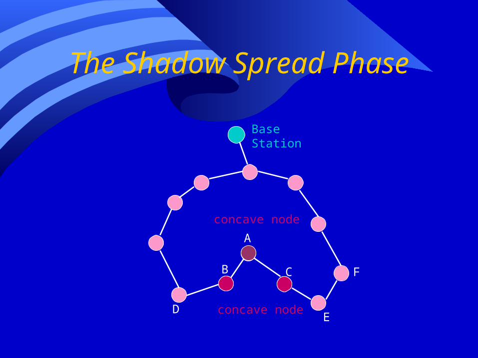
The Shadow Spread Phase
Base Station
A
B C
DE
F
concave node
concave node
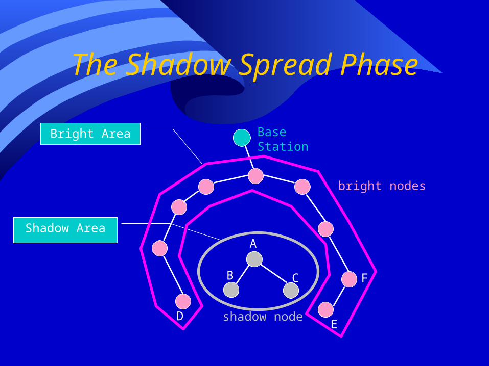
The Shadow Spread Phase
Base Station
A
B C
DE
F
shadow node
bright nodes
Shadow Area
Bright Area

The Shadow Spread Phase
• Nodes exchange information by means of periodically broadcasting beacon messages beacon(status, location)
• the shadow spread phase converges in n rounds in terms of beacon broadcast interval B

The Cost Spread Phase
5
12
7
16
20
Base Station
18
8
15
16
2019
23
A
B C
DE
F
Euclidian distance to the BS
19+∆
∆ should be set to the average Euclidean distance between neighboring sensor nodes
∆ is set to 3 in this example
22

The Cost Spread Phase
5
12
7
16
20
Base Station
18
8
15
16
2019
23
A
B C
DE
F
22+∆
22
25

The Cost Spread Phase
5
12
7
16
20
Base Station
18
8
15
16
2019
23
A
B C
DE
F
23+∆
22
25 26
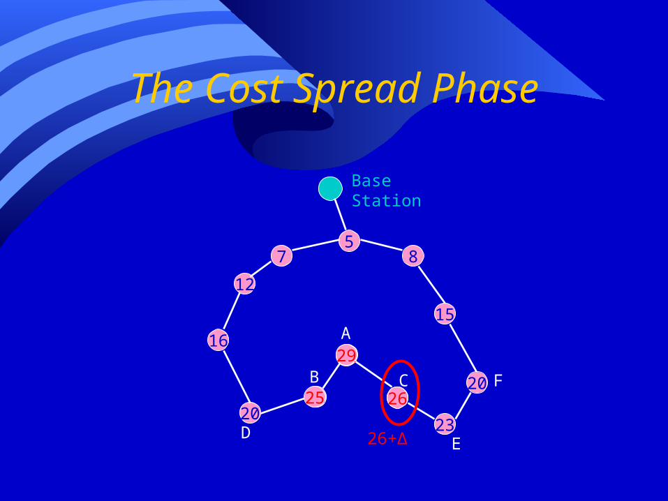
The Cost Spread Phase
5
12
7
16
20
Base Station
18
8
15
16
2019
23
A
B C
DE
F
26+∆
2625
2229

The Cost Spread Phase
• Once the status of a sensor node turns from bright to shadow, the cost spread phase can be triggered on that node immediately
• The convergence length of the cost spread algorithm in the whole sensor network is only associated with the maximum size of these shadow areas
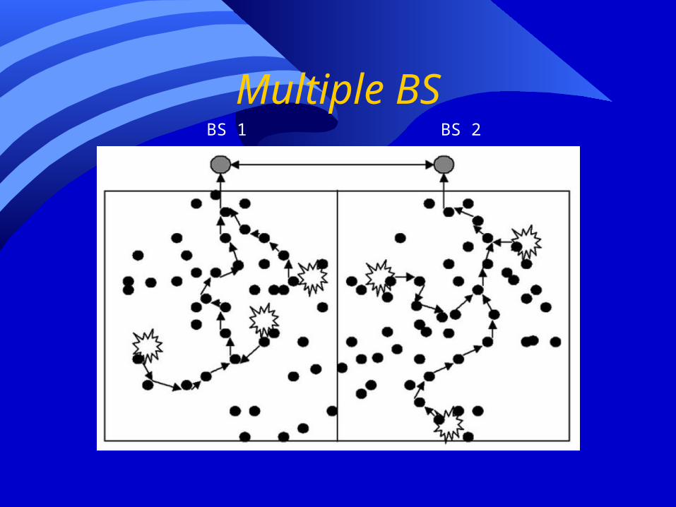
Multiple BSBS 1 BS 2

PAGER-M
The shadow spread and cost spread processes begin
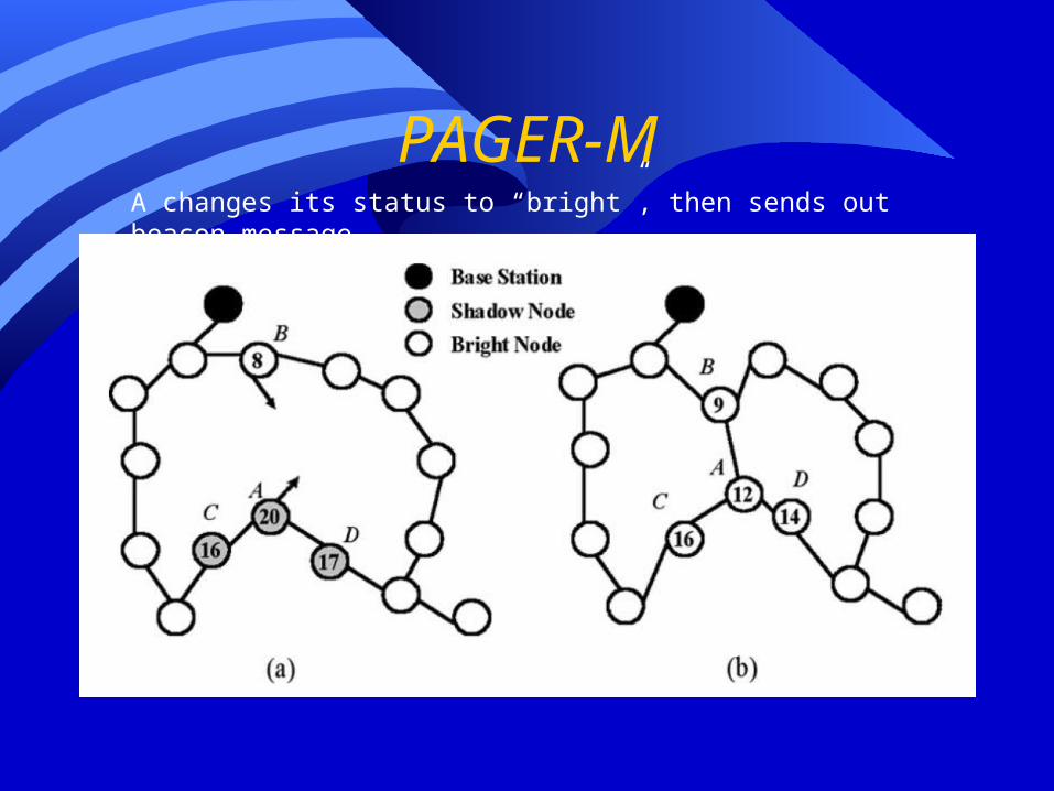
PAGER-MA changes its status to “bright”, then sends out beacon message

Path Redundancy
• We use path redundancy to reduce forwarding failure• Choosing the neighbor with closest arrival time among available forwarding candidates

Simulation ~PAGER-S
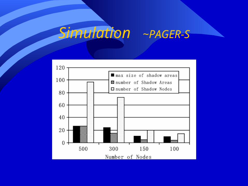
Simulation ~PAGER-S

Simulation ~PAGER-S

Simulation ~PAGER-S

Simulation ~PAGER-M

Simulation ~PAGER-M

Simulation ~PAGER-M

Conclusions
• PAGER has the loop free guarantee delivery property
• The mobility adaptability of PAGE make it suitable for use in mobile sensor networks with frequent topology changes