Embed Size (px)
Citation preview
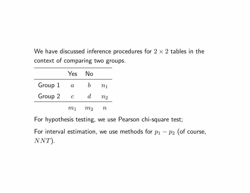
We have discussed inference procedures for 2 × 2 tables in the
context of comparing two groups.
Yes No
Group 1 a b n1
Group 2 c d n2
m1 m2 n
For hypothesis testing, we use Pearson chi-square test;
For interval estimation, we use methods for p1 − p2 (of course,
NNT ).

However, Pearson chi-square test will work only if expected value for
every cell is greater than 5.
For data with small cells, we can use Fisher’s ‘exact’ test. The idea of
this test is to fix the row and column totals as the observed table, and
compute the probabilities of observing as or more extreme tables in their
departure from the null hypothesis (recall the definition of P -value).
Fisher (1935, The logic of inductive inference JRSS A 98: 39-54)
presented his test at the annual Christmas meeting of the Royal
Statistical Society.
The title is very good, because I’ve heard that the most important
contribution of statistics to science is not the formula, but logic.
Still, right after his talk, a speaker compared Fisher’s talk to “the
braying of the Golden Ass”.
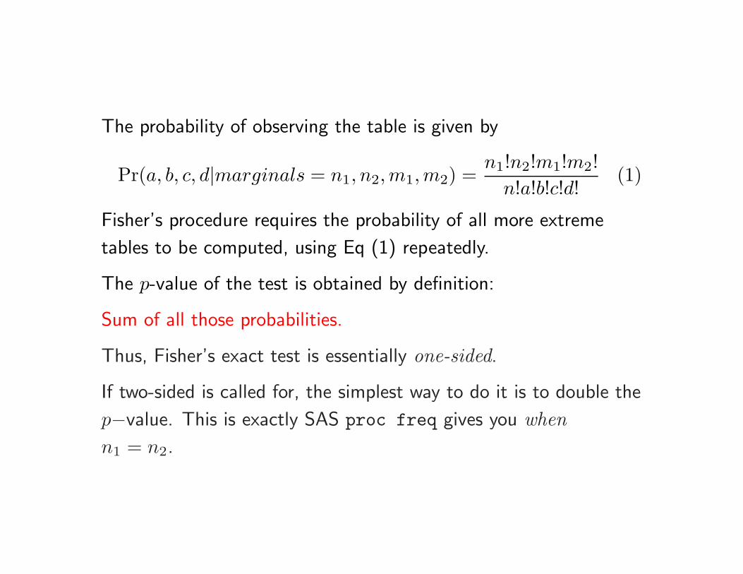
The probability of observing the table is given by
Pr(a, b, c, d|marginals = n1, n2, m1, m2) =n1!n2!m1!m2!
n!a!b!c!d!(1)
Fisher’s procedure requires the probability of all more extreme
tables to be computed, using Eq (1) repeatedly.
The p-value of the test is obtained by definition:
Sum of all those probabilities.
Thus, Fisher’s exact test is essentially one-sided.
If two-sided is called for, the simplest way to do it is to double the
p−value. This is exactly SAS proc freq gives you whenn1 = n2.
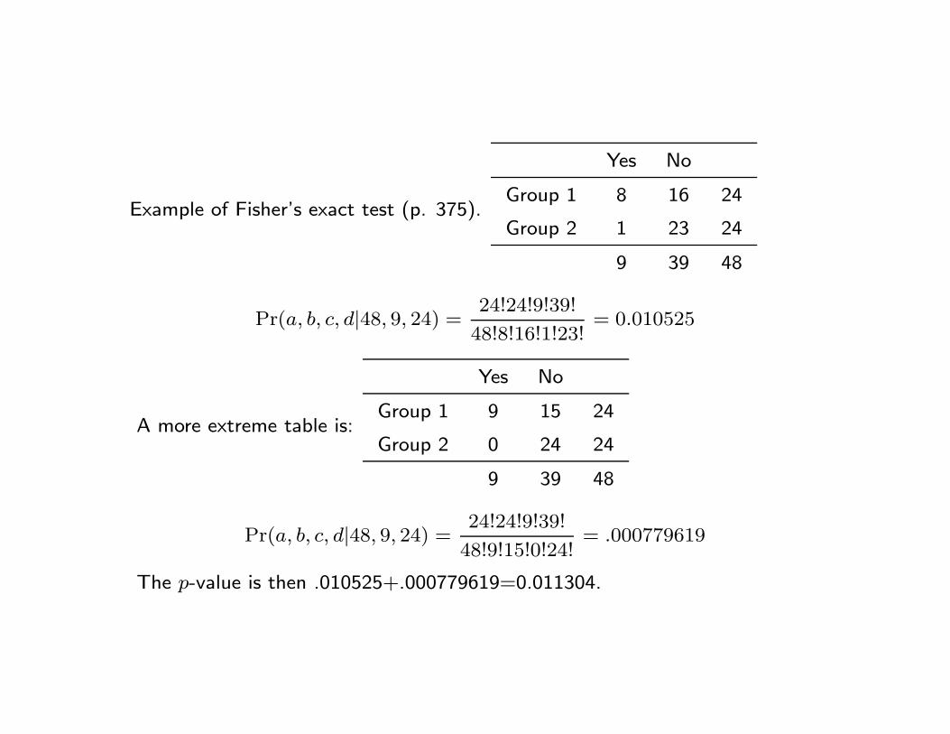
Example of Fisher’s exact test (p. 375).
Yes No
Group 1 8 16 24
Group 2 1 23 24
9 39 48
Pr(a, b, c, d|48, 9, 24) =24!24!9!39!
48!8!16!1!23!= 0.010525
A more extreme table is:
Yes No
Group 1 9 15 24
Group 2 0 24 24
9 39 48
Pr(a, b, c, d|48, 9, 24) =24!24!9!39!
48!9!15!0!24!= .000779619
The p-value is then .010525+.000779619=0.011304.
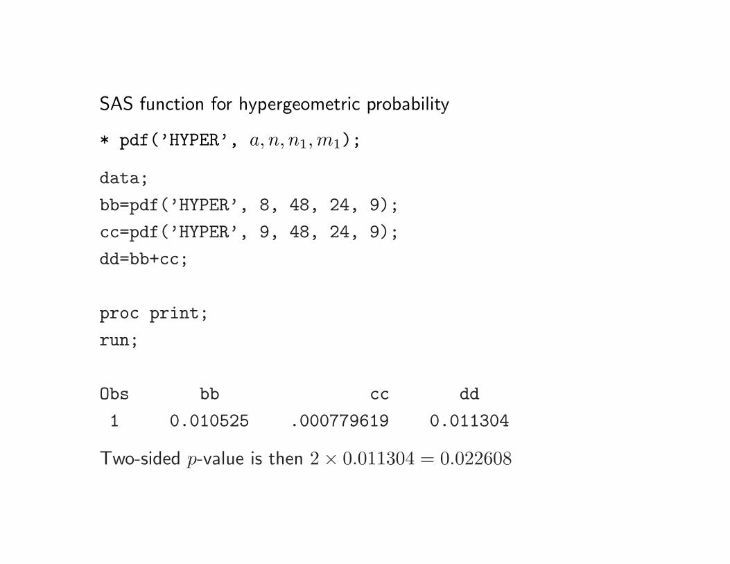
SAS function for hypergeometric probability
* pdf(’HYPER’, a, n, n1, m1);
data;
bb=pdf(’HYPER’, 8, 48, 24, 9);
cc=pdf(’HYPER’, 9, 48, 24, 9);
dd=bb+cc;
proc print;
run;
Obs bb cc dd
1 0.010525 .000779619 0.011304
Two-sided p-value is then 2 × 0.011304 = 0.022608
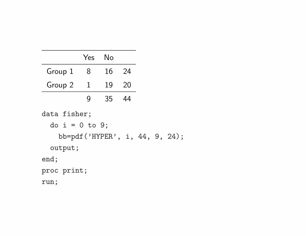
Yes No
Group 1 8 16 24
Group 2 1 19 20
9 35 44
data fisher;
do i = 0 to 9;
bb=pdf(’HYPER’, i, 44, 9, 24);
output;
end;
proc print;
run;
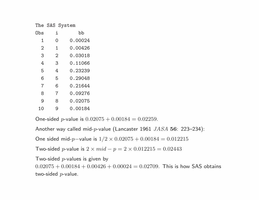
The SAS System
Obs i bb
1 0 0.00024
2 1 0.00426
3 2 0.03018
4 3 0.11066
5 4 0.23239
6 5 0.29048
7 6 0.21644
8 7 0.09276
9 8 0.02075
10 9 0.00184
One-sided p-value is 0.02075 + 0.00184 = 0.02259.
Another way called mid-p-value (Lancaster 1961 JASA 56: 223–234):
One sided mid-p−value is 1/2 × 0.02075 + 0.00184 = 0.012215
Two-sided p-value is 2 × mid − p = 2 × 0.012215 = 0.02443
Two-sided p-values is given by
0.02075 + 0.00184 + 0.00426 + 0.00024 = 0.02709. This is how SAS obtains
two-sided p-value.
The way to present the results is: Rate in group I was ? , in Group
II was ?; difference ? (95% confidence interval ? to ? ), P = ?
(Fisher’s Exact test two-sided mid P).
McKinney et al (1989 The inexact use of Fisher’s exact test in six
major medical journals JAMA 261:3430–3433).
Half of 70 articles reviewed either had used a one-tailed test when
a two-tailed test was called for, or the authors simply had not
bothered to state which test they had used.
If only hypothesis testing, an epidemiologist’s life would be too
easy.
Effect estimation makes it hard, also interesting.
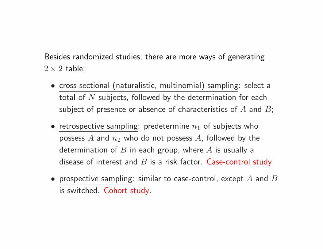
Besides randomized studies, there are more ways of generating
2 × 2 table:
• cross-sectional (naturalistic, multinomial) sampling: select a
total of N subjects, followed by the determination for each
subject of presence or absence of characteristics of A and B;
• retrospective sampling: predetermine n1 of subjects who
possess A and n2 who do not possess A, followed by the
determination of B in each group, where A is usually a
disease of interest and B is a risk factor. Case-control study
• prospective sampling: similar to case-control, except A and B
is switched. Cohort study.
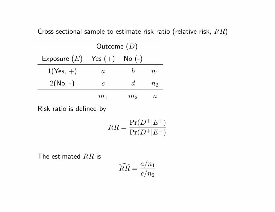
Cross-sectional sample to estimate risk ratio (relative risk, RR)
Outcome (D)
Exposure (E) Yes (+) No (-)
1(Yes, +) a b n1
2(No, -) c d n2
m1 m2 n
Risk ratio is defined by
RR =Pr(D+|E+)Pr(D+|E−)
The estimated RR is
RR =a/n1
c/n2
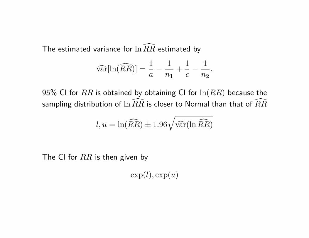
The estimated variance for ln RR estimated by
var[ln(RR)] =1a− 1
n1+
1c− 1
n2.
95% CI for RR is obtained by obtaining CI for ln(RR) because the
sampling distribution of ln RR is closer to Normal than that of RR
l, u = ln(RR) ± 1.96√
var(ln RR)
The CI for RR is then given by
exp(l), exp(u)
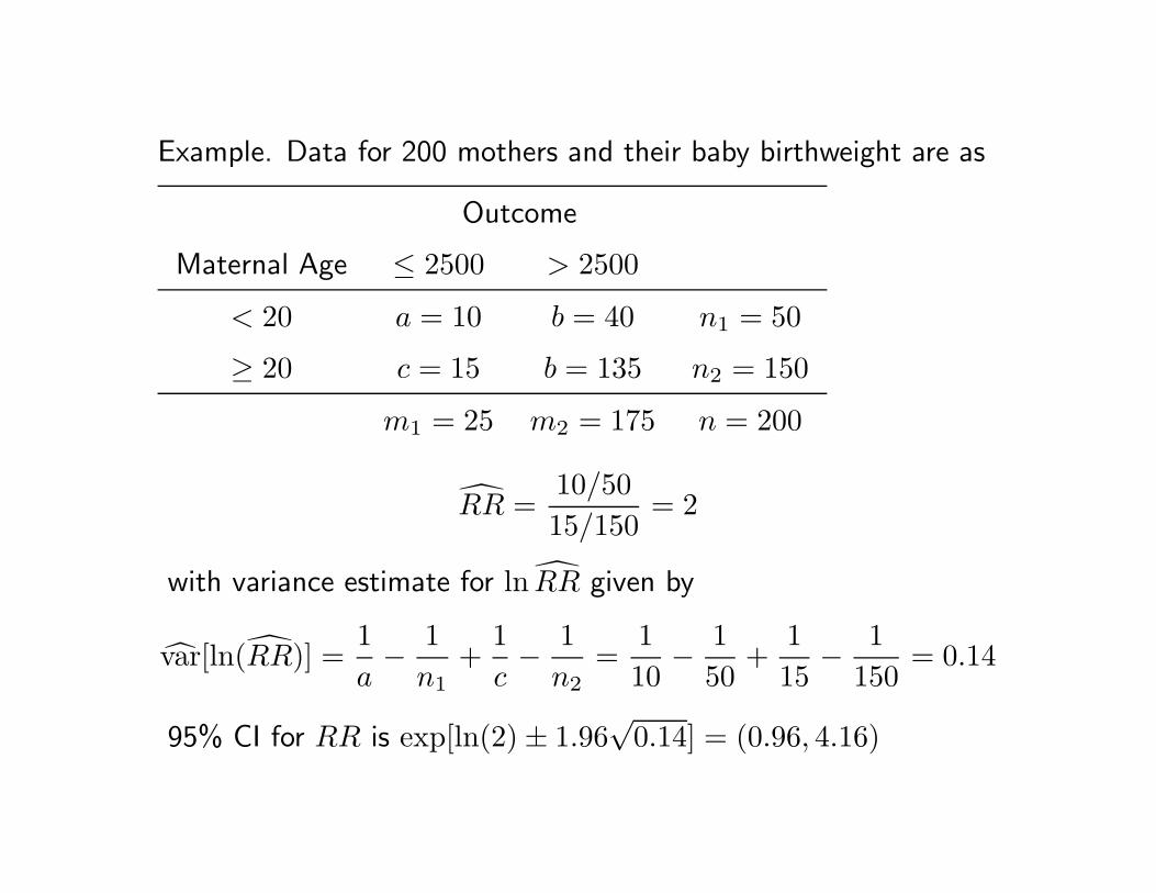
Example. Data for 200 mothers and their baby birthweight are as
Outcome
Maternal Age ≤ 2500 > 2500
< 20 a = 10 b = 40 n1 = 50
≥ 20 c = 15 b = 135 n2 = 150
m1 = 25 m2 = 175 n = 200
RR =10/5015/150
= 2
with variance estimate for ln RR given by
var[ln(RR)] =1a− 1
n1+
1c− 1
n2=
110
− 150
+115
− 1150
= 0.14
95% CI for RR is exp[ln(2) ± 1.96√
0.14] = (0.96, 4.16)
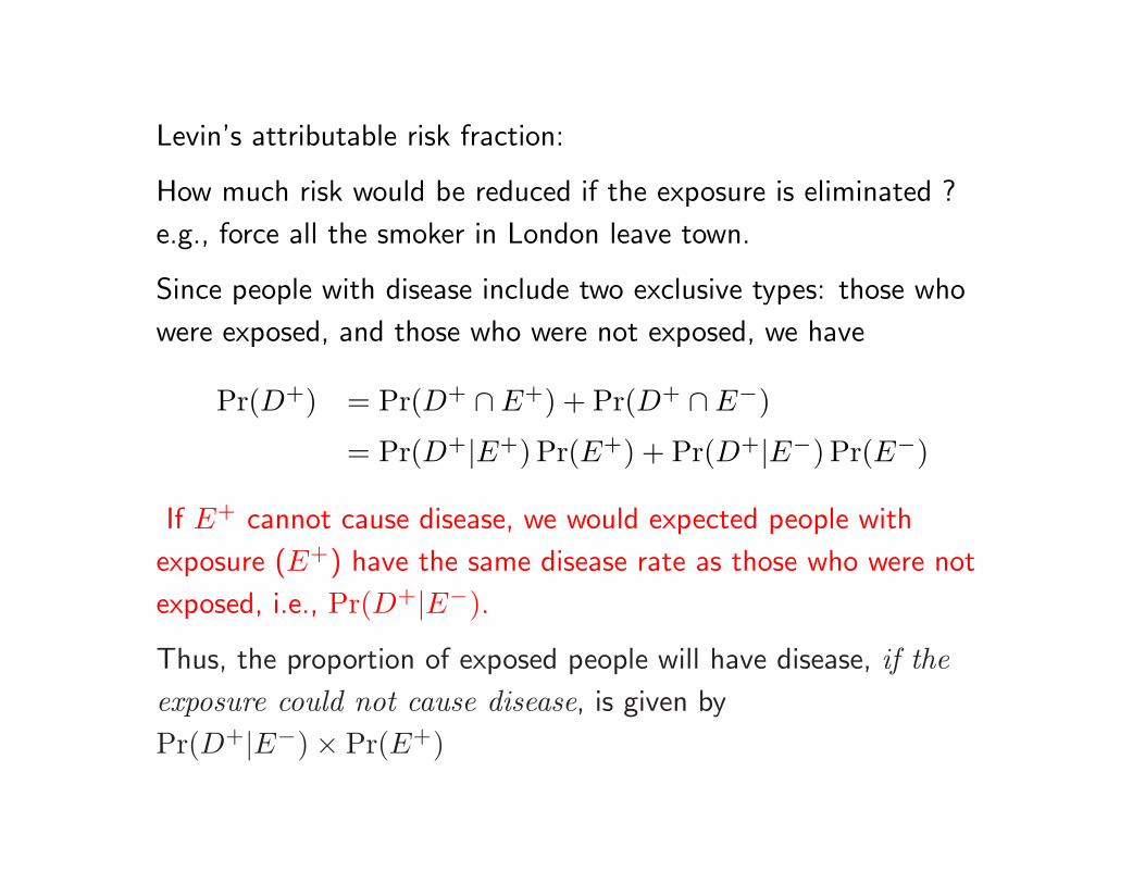
Levin’s attributable risk fraction:
How much risk would be reduced if the exposure is eliminated ?
e.g., force all the smoker in London leave town.
Since people with disease include two exclusive types: those who
were exposed, and those who were not exposed, we have
Pr(D+) = Pr(D+ ∩ E+) + Pr(D+ ∩ E−)
= Pr(D+|E+) Pr(E+) + Pr(D+|E−) Pr(E−)
If E+ cannot cause disease, we would expected people with
exposure (E+) have the same disease rate as those who were not
exposed, i.e., Pr(D+|E−).
Thus, the proportion of exposed people will have disease, if theexposure could not cause disease, is given by
Pr(D+|E−) × Pr(E+)
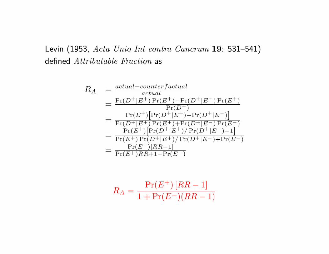
Levin (1953, Acta Unio Int contra Cancrum 19: 531–541)
defined Attributable Fraction as
RA = actual−counterfactualactual
= Pr(D+|E+) Pr(E+)−Pr(D+|E−) Pr(E+)Pr(D+)
=Pr(E+)[Pr(D+|E+)−Pr(D+|E−)]
Pr(D+|E+) Pr(E+)+Pr(D+|E−) Pr(E−)
=Pr(E+)[Pr(D+|E+)/ Pr(D+|E−)−1]
Pr(E+) Pr(D+|E+)/ Pr(D+|E−)+Pr(E−)
= Pr(E+)[RR−1]Pr(E+)RR+1−Pr(E−)
RA =Pr(E+) [RR − 1]
1 + Pr(E+)(RR − 1)
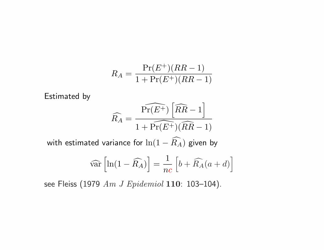
RA =Pr(E+)(RR − 1)
1 + Pr(E+)(RR − 1)
Estimated by
RA =Pr(E+)
[RR − 1
]1 + Pr(E+)(RR − 1)
with estimated variance for ln(1 − RA) given by
var[ln(1 − RA)
]=
1nc
[b + RA(a + d)
]see Fleiss (1979 Am J Epidemiol 110: 103–104).
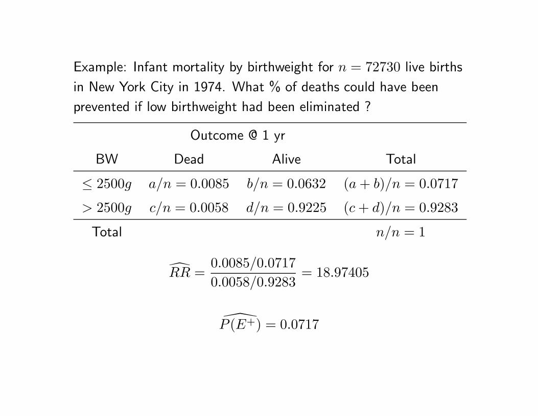
Example: Infant mortality by birthweight for n = 72730 live births
in New York City in 1974. What % of deaths could have been
prevented if low birthweight had been eliminated ?
Outcome @ 1 yr
BW Dead Alive Total
≤ 2500g a/n = 0.0085 b/n = 0.0632 (a + b)/n = 0.0717
> 2500g c/n = 0.0058 d/n = 0.9225 (c + d)/n = 0.9283
Total n/n = 1
RR =0.0085/0.07170.0058/0.9283
= 18.97405
P (E+) = 0.0717
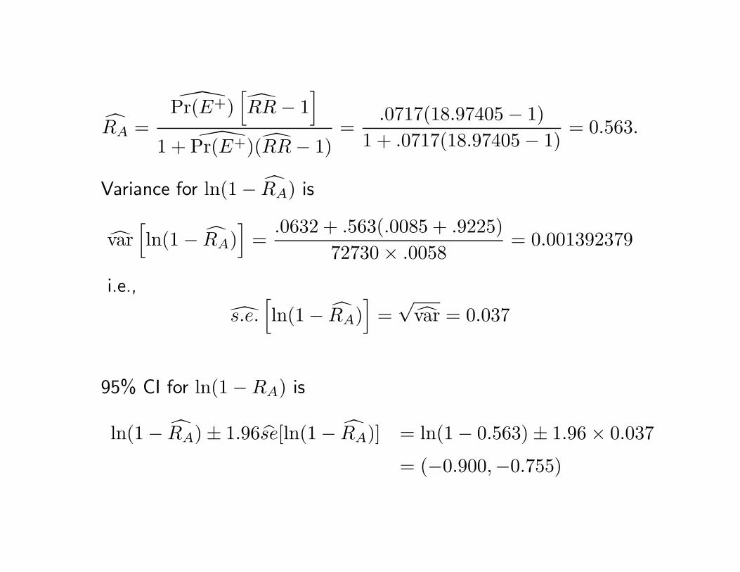
RA =Pr(E+)
[RR − 1
]1 + Pr(E+)(RR − 1)
=.0717(18.97405 − 1)
1 + .0717(18.97405 − 1)= 0.563.
Variance for ln(1 − RA) is
var[ln(1 − RA)
]=
.0632 + .563(.0085 + .9225)72730 × .0058
= 0.001392379
i.e.,
s.e.[ln(1 − RA)
]=
√var = 0.037
95% CI for ln(1 − RA) is
ln(1 − RA) ± 1.96se[ln(1 − RA)] = ln(1 − 0.563) ± 1.96 × 0.037
= (−0.900,−0.755)
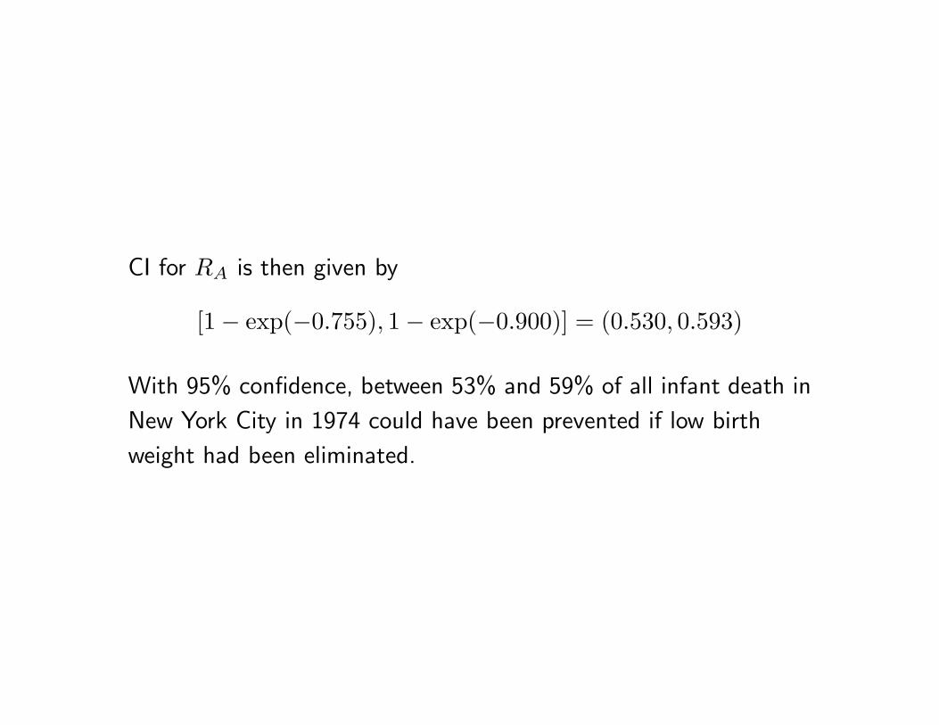
CI for RA is then given by
[1 − exp(−0.755), 1 − exp(−0.900)] = (0.530, 0.593)
With 95% confidence, between 53% and 59% of all infant death in
New York City in 1974 could have been prevented if low birth
weight had been eliminated.
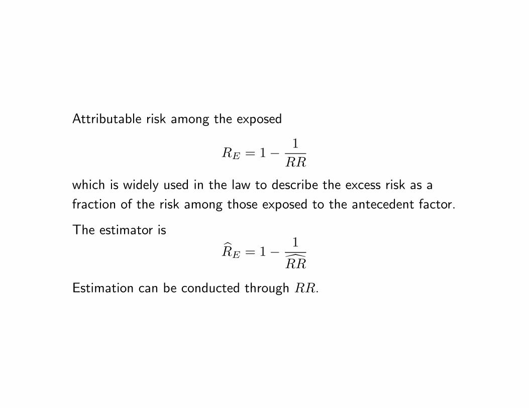
Attributable risk among the exposed
RE = 1 − 1RR
which is widely used in the law to describe the excess risk as a
fraction of the risk among those exposed to the antecedent factor.
The estimator is
RE = 1 − 1
RR
Estimation can be conducted through RR.

.
Cohort study may be used to estimate all of the above effect
measures.
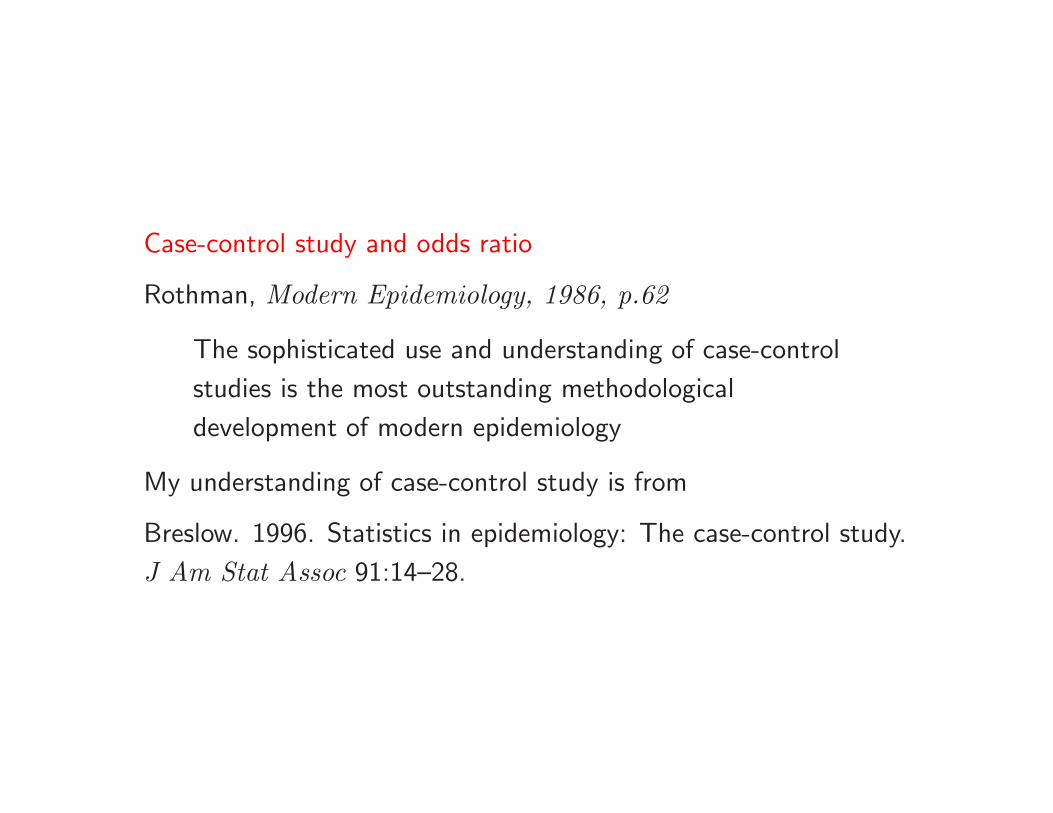
Case-control study and odds ratio
Rothman, Modern Epidemiology, 1986, p.62
The sophisticated use and understanding of case-control
studies is the most outstanding methodological
development of modern epidemiology
My understanding of case-control study is from
Breslow. 1996. Statistics in epidemiology: The case-control study.
J Am Stat Assoc 91:14–28.
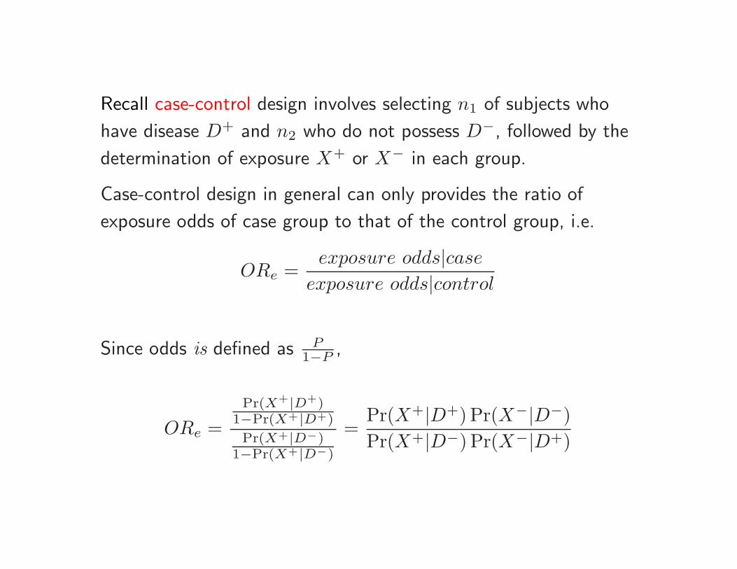
Recall case-control design involves selecting n1 of subjects who
have disease D+ and n2 who do not possess D−, followed by the
determination of exposure X+ or X− in each group.
Case-control design in general can only provides the ratio of
exposure odds of case group to that of the control group, i.e.
ORe =exposure odds|case
exposure odds|control
Since odds is defined as P1−P ,
ORe =Pr(X+|D+)
1−Pr(X+|D+)
Pr(X+|D−)1−Pr(X+|D−)
=Pr(X+|D+) Pr(X−|D−)Pr(X+|D−) Pr(X−|D+)
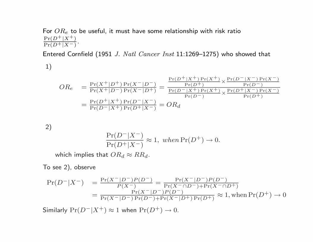
For ORe to be useful, it must have some relationship with risk ratioPr(D+|X+)
Pr(D+|X−).
Entered Cornfield (1951 J. Natl Cancer Inst 11:1269–1275) who showed that
1)
ORe =Pr(X+|D+) Pr(X−|D−)
Pr(X+|D−) Pr(X−|D+)=
Pr(D+|X+) Pr(X+)Pr(D+)
×Pr(D−|X−) Pr(X−)Pr(D−)
Pr(D−|X+) Pr(X+)Pr(D−)
×Pr(D+|X−) Pr(X−)Pr(D+)
=Pr(D+|X+) Pr(D−|X−)
Pr(D−|X+) Pr(D+|X−)= ORd
2)
Pr(D−|X−)
Pr(D+|X−)≈ 1, when Pr(D+) → 0.
which implies that ORd ≈ RRd.
To see 2), observe
Pr(D−|X−) =Pr(X−|D−)P (D−)
P (X−)=
Pr(X−|D−)P (D−)
Pr(X−∩D−)+Pr(X−∩D+)
=Pr(X−|D−)P (D−)
Pr(X−|D−) Pr(D−)+Pr(X−|D+) Pr(D+)≈ 1, whenPr(D+) → 0
Similarly Pr(D−|X+) ≈ 1 when Pr(D+) → 0.
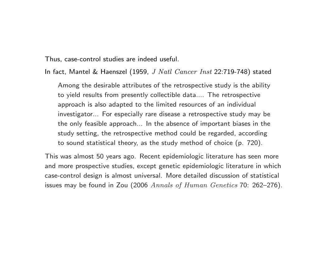
Thus, case-control studies are indeed useful.
In fact, Mantel & Haenszel (1959, J Natl Cancer Inst 22:719-748) stated
Among the desirable attributes of the retrospective study is the ability
to yield results from presently collectible data.... The retrospective
approach is also adapted to the limited resources of an individual
investigator... For especially rare disease a retrospective study may be
the only feasible approach... In the absence of important biases in the
study setting, the retrospective method could be regarded, according
to sound statistical theory, as the study method of choice (p. 720).
This was almost 50 years ago. Recent epidemiologic literature has seen more
and more prospective studies, except genetic epidemiologic literature in which
case-control design is almost universal. More detailed discussion of statistical
issues may be found in Zou (2006 Annals of Human Genetics 70: 262–276).
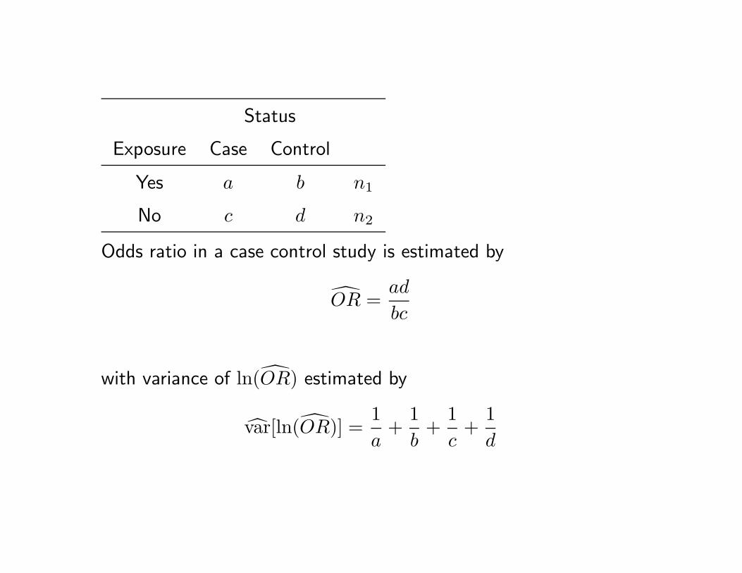
Status
Exposure Case Control
Yes a b n1
No c d n2
Odds ratio in a case control study is estimated by
OR =ad
bc
with variance of ln(OR) estimated by
var[ln(OR)] =1a
+1b
+1c
+1d
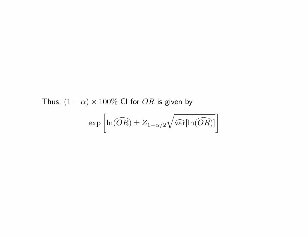
Thus, (1 − α) × 100% CI for OR is given by
exp[ln(OR) ± Z1−α/2
√var[ln(OR)]
]
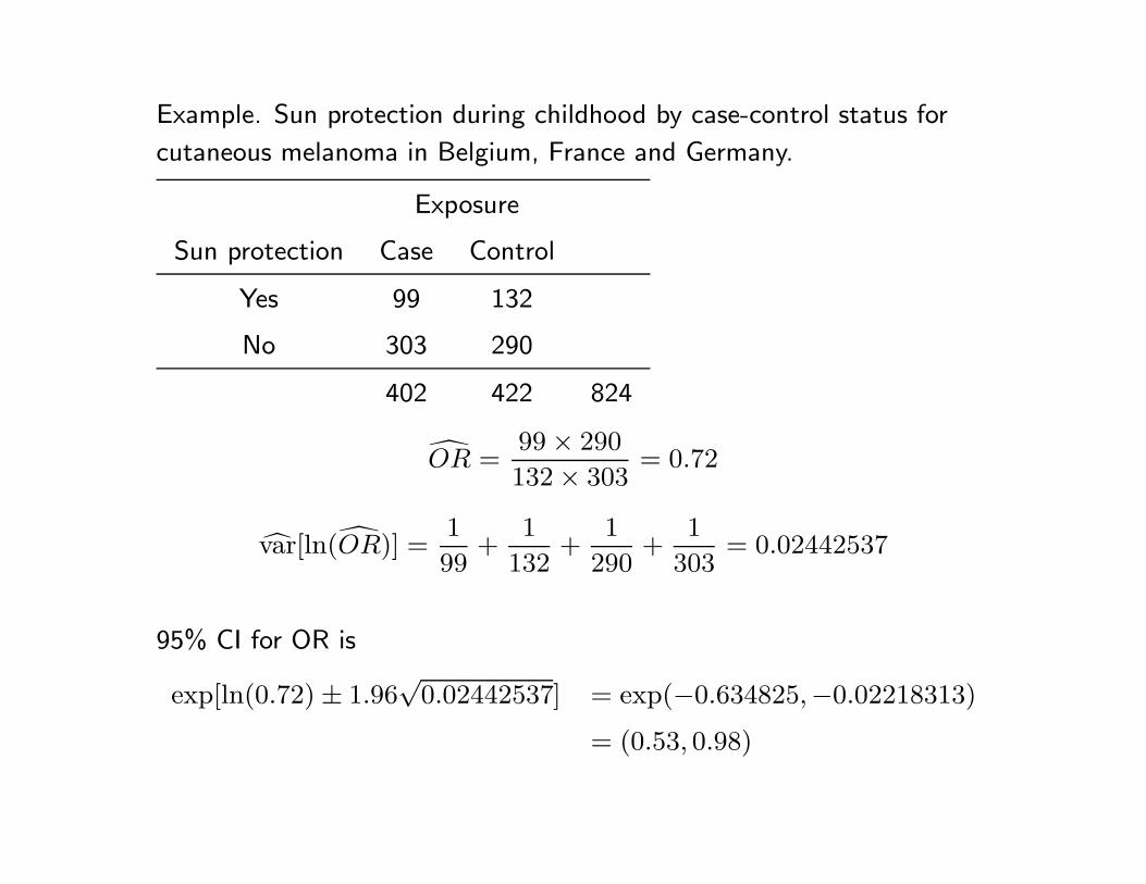
Example. Sun protection during childhood by case-control status for
cutaneous melanoma in Belgium, France and Germany.
Exposure
Sun protection Case Control
Yes 99 132
No 303 290
402 422 824
OR =99 × 290
132 × 303= 0.72
var[ln(OR)] =1
99+
1
132+
1
290+
1
303= 0.02442537
95% CI for OR is
exp[ln(0.72) ± 1.96√
0.02442537] = exp(−0.634825,−0.02218313)
= (0.53, 0.98)
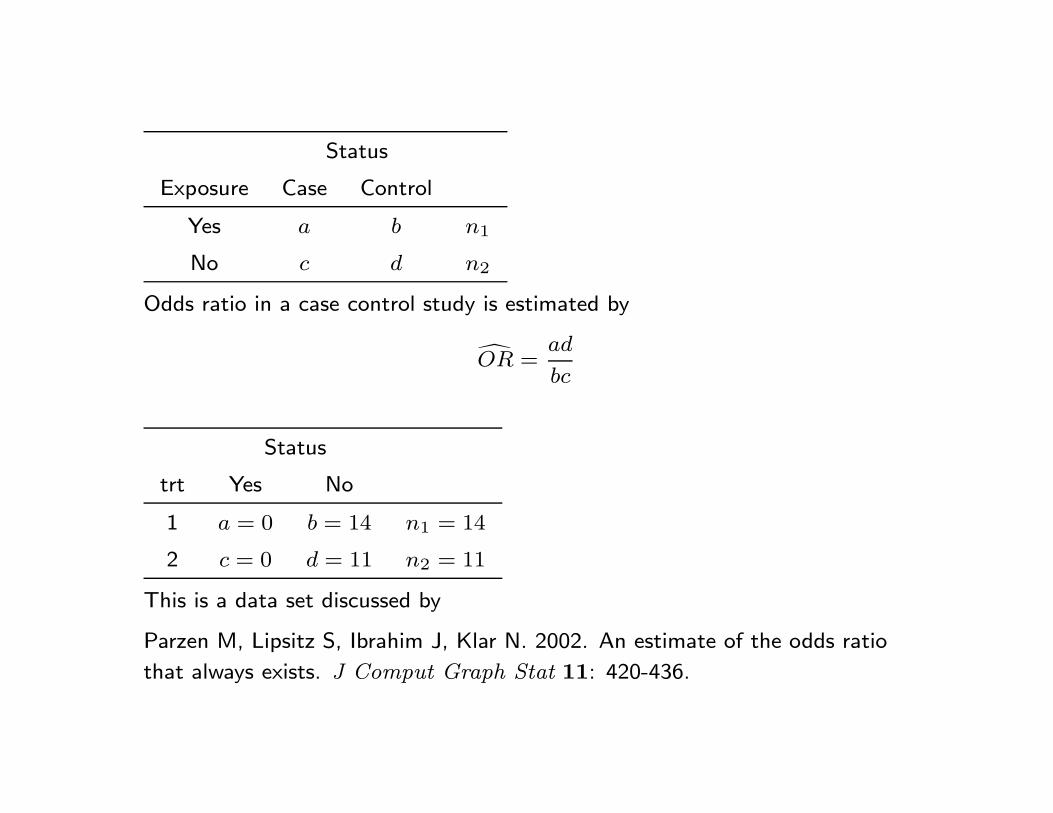
Status
Exposure Case Control
Yes a b n1
No c d n2
Odds ratio in a case control study is estimated by
OR =ad
bc
Status
trt Yes No
1 a = 0 b = 14 n1 = 14
2 c = 0 d = 11 n2 = 11
This is a data set discussed by
Parzen M, Lipsitz S, Ibrahim J, Klar N. 2002. An estimate of the odds ratio
that always exists. J Comput Graph Stat 11: 420-436.
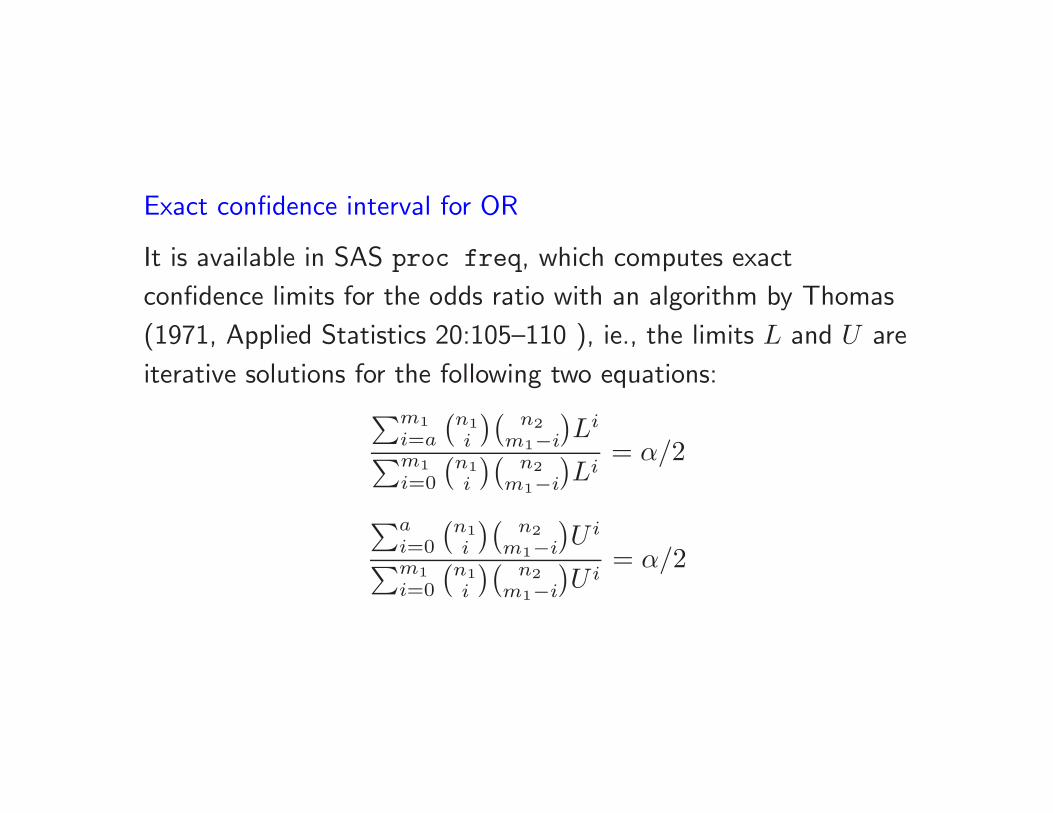
Exact confidence interval for OR
It is available in SAS proc freq, which computes exact
confidence limits for the odds ratio with an algorithm by Thomas
(1971, Applied Statistics 20:105–110 ), ie., the limits L and U are
iterative solutions for the following two equations:∑m1i=a
(n1i
)(n2
m1−i
)Li∑m1
i=0
(n1i
)(n2
m1−i
)Li
= α/2
∑ai=0
(n1i
)(n2
m1−i
)U i∑m1
i=0
(n1i
)(n2
m1−i
)U i
= α/2
Exact may not be the best in categorical data analysis because the results may
be too conservative
Agresti A. 2003. Dealing with discreteness: making ’exact’ confidence
intervals for proportions, differences of proportions, and odds ratios more
exact Stat Meth Med Res 12 (1): 3–21.
... the inversion of the asymptotic score test seems to be a good
choice. This tends to have actual level fluctuating around the
nominal level. If one prefers that level to be a bit more conservative,
mid-p adaptations of exact methods work well. For situations that
require a bound on the error, it appears that basing conservative
intervals on inverting the exact score test has reasonable
performance. For teaching, the Wald-type interval of point estimate
plus and minus a normal-score multiple of a standard error is
simplest. Unfortunately, this can perform poorly, but simple
adjustments sometimes provide much improved performance.
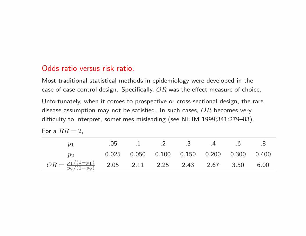
Odds ratio versus risk ratio.
Most traditional statistical methods in epidemiology were developed in the
case of case-control design. Specifically, OR was the effect measure of choice.
Unfortunately, when it comes to prospective or cross-sectional design, the rare
disease assumption may not be satisfied. In such cases, OR becomes very
difficulty to interpret, sometimes misleading (see NEJM 1999;341:279–83).
For a RR = 2,
p1 .05 .1 .2 .3 .4 .6 .8
p2 0.025 0.050 0.100 0.150 0.200 0.300 0.400
OR =p1/(1−p1)p2/(1−p2)
2.05 2.11 2.25 2.43 2.67 3.50 6.00
My view is that we must always remember why Cornfield (1951)
proposed OR.
Excellent discussion on the choice of effect measures may be found
in Greenland (Interpretation and choice of effect measures in
epidemiologic analyses. Am J Epidemiol 1987;125:761–8).
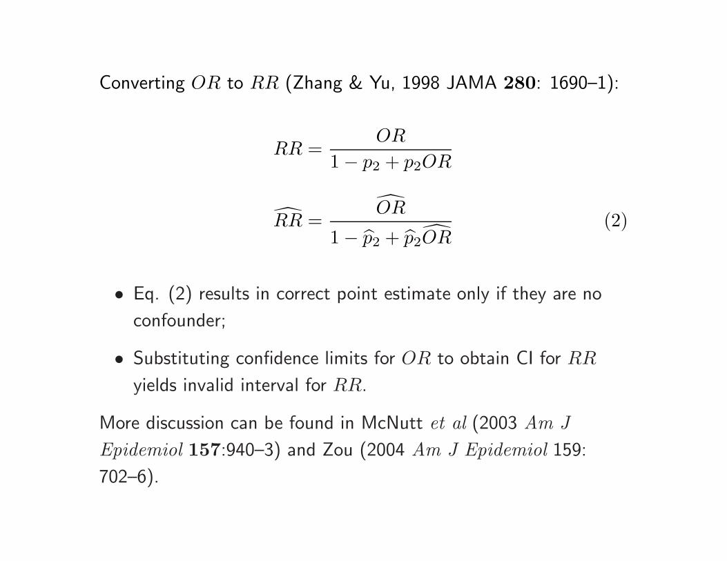
Converting OR to RR (Zhang & Yu, 1998 JAMA 280: 1690–1):
RR =OR
1 − p2 + p2OR
RR =OR
1 − p2 + p2OR(2)
• Eq. (2) results in correct point estimate only if they are no
confounder;
• Substituting confidence limits for OR to obtain CI for RR
yields invalid interval for RR.
More discussion can be found in McNutt et al (2003 Am JEpidemiol 157:940–3) and Zou (2004 Am J Epidemiol 159:
702–6).
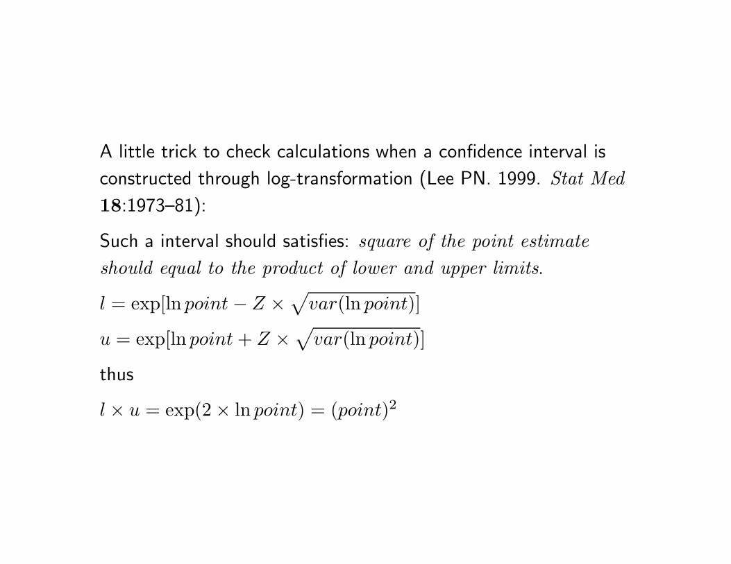
A little trick to check calculations when a confidence interval is
constructed through log-transformation (Lee PN. 1999. Stat Med18:1973–81):
Such a interval should satisfies: square of the point estimateshould equal to the product of lower and upper limits.
l = exp[ln point − Z × √var(ln point)]
u = exp[ln point + Z × √var(ln point)]
thus
l × u = exp(2 × ln point) = (point)2
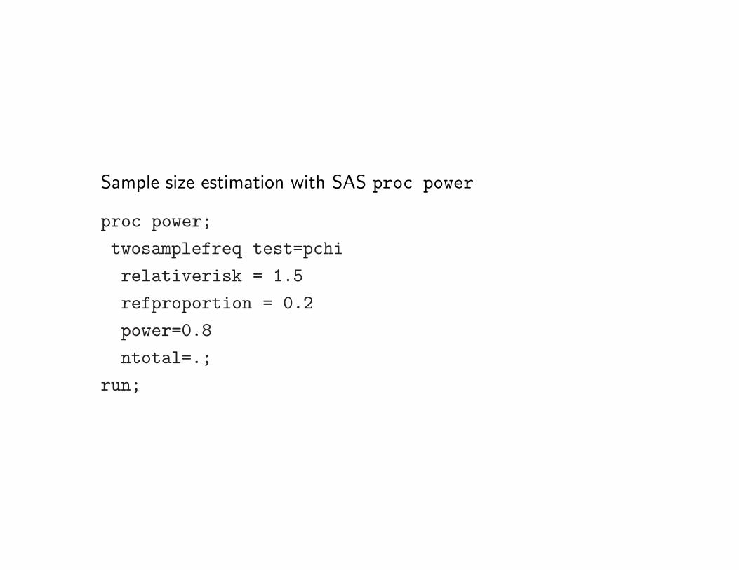
Sample size estimation with SAS proc power
proc power;
twosamplefreq test=pchi
relativerisk = 1.5
refproportion = 0.2
power=0.8
ntotal=.;
run;
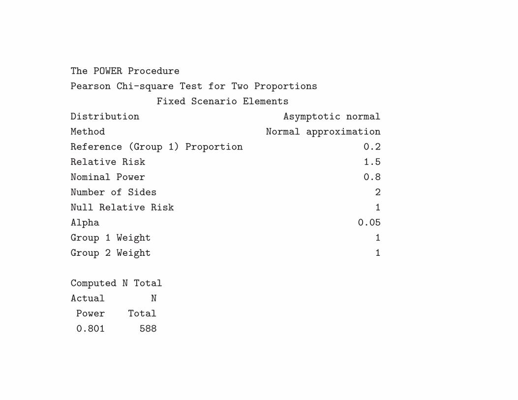
The POWER Procedure
Pearson Chi-square Test for Two Proportions
Fixed Scenario Elements
Distribution Asymptotic normal
Method Normal approximation
Reference (Group 1) Proportion 0.2
Relative Risk 1.5
Nominal Power 0.8
Number of Sides 2
Null Relative Risk 1
Alpha 0.05
Group 1 Weight 1
Group 2 Weight 1
Computed N Total
Actual N
Power Total
0.801 588
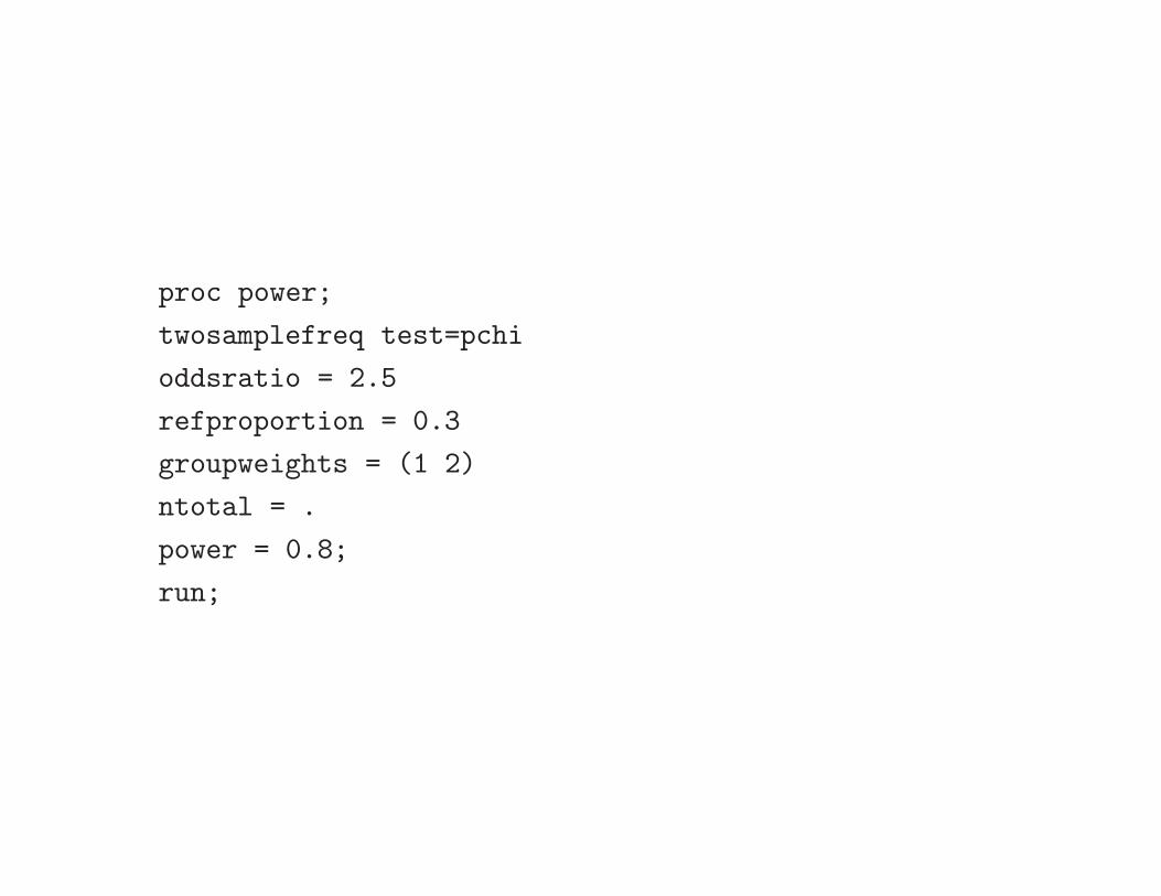
proc power;
twosamplefreq test=pchi
oddsratio = 2.5
refproportion = 0.3
groupweights = (1 2)
ntotal = .
power = 0.8;
run;
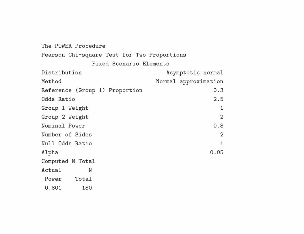
The POWER Procedure
Pearson Chi-square Test for Two Proportions
Fixed Scenario Elements
Distribution Asymptotic normal
Method Normal approximation
Reference (Group 1) Proportion 0.3
Odds Ratio 2.5
Group 1 Weight 1
Group 2 Weight 2
Nominal Power 0.8
Number of Sides 2
Null Odds Ratio 1
Alpha 0.05
Computed N Total
Actual N
Power Total
0.801 180
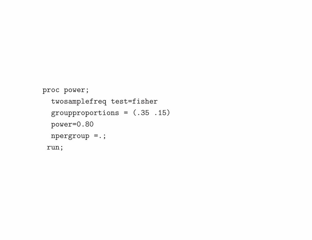
proc power;
twosamplefreq test=fisher
groupproportions = (.35 .15)
power=0.80
npergroup =.;
run;
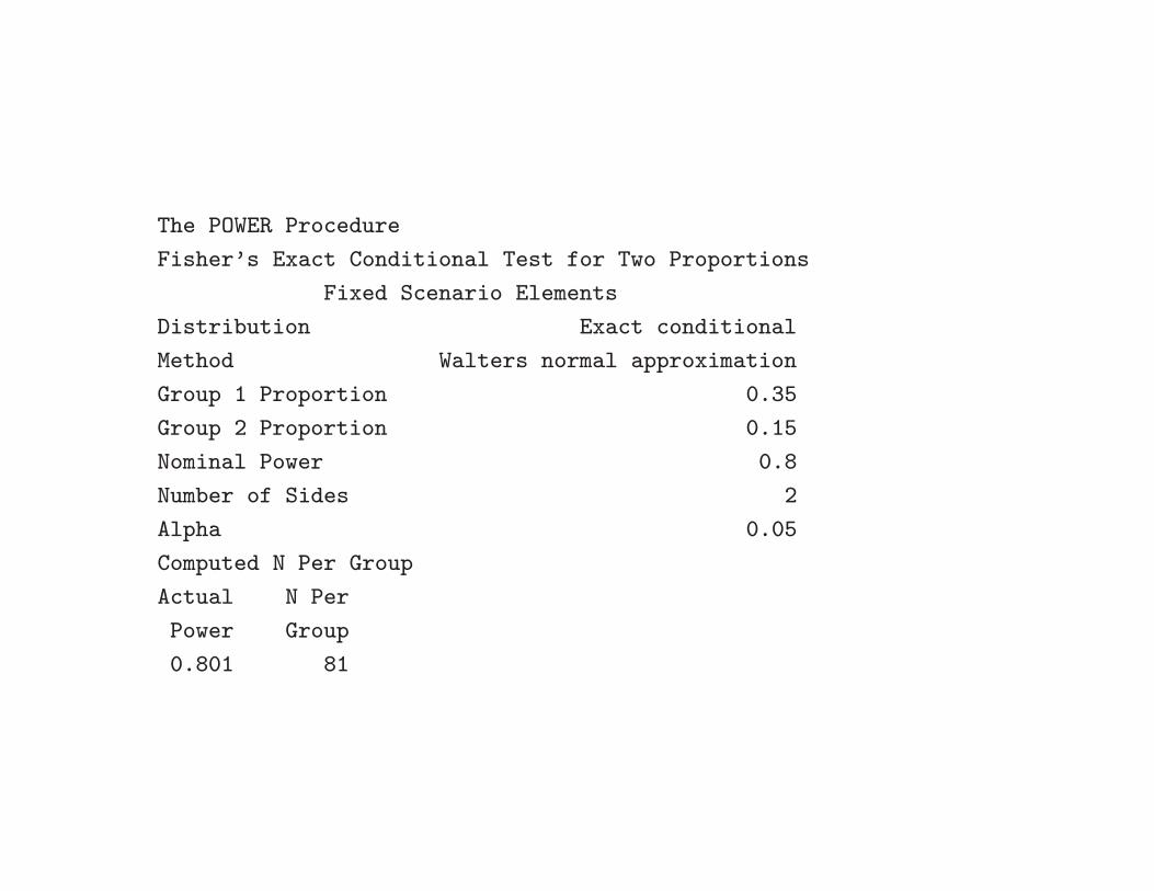
The POWER Procedure
Fisher’s Exact Conditional Test for Two Proportions
Fixed Scenario Elements
Distribution Exact conditional
Method Walters normal approximation
Group 1 Proportion 0.35
Group 2 Proportion 0.15
Nominal Power 0.8
Number of Sides 2
Alpha 0.05
Computed N Per Group
Actual N Per
Power Group
0.801 81

’
Combine information from multiple 2 × 2tables (Mantel-Haenszel methods)
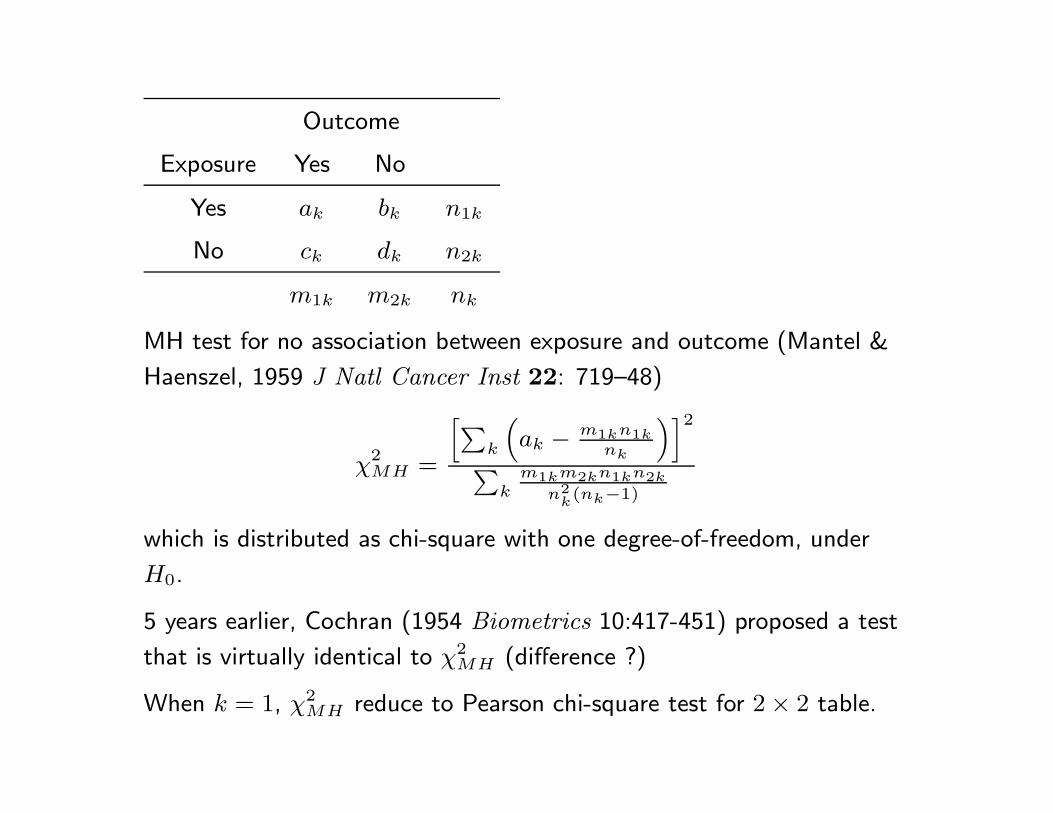
Outcome
Exposure Yes No
Yes ak bk n1k
No ck dk n2k
m1k m2k nk
MH test for no association between exposure and outcome (Mantel &
Haenszel, 1959 J Natl Cancer Inst 22: 719–48)
χ2MH =
[∑k
(ak − m1kn1k
nk
)]2
∑k
m1km2kn1kn2k
n2k(nk−1)
which is distributed as chi-square with one degree-of-freedom, under
H0.
5 years earlier, Cochran (1954 Biometrics 10:417-451) proposed a test
that is virtually identical to χ2MH (difference ?)
When k = 1, χ2MH reduce to Pearson chi-square test for 2 × 2 table.
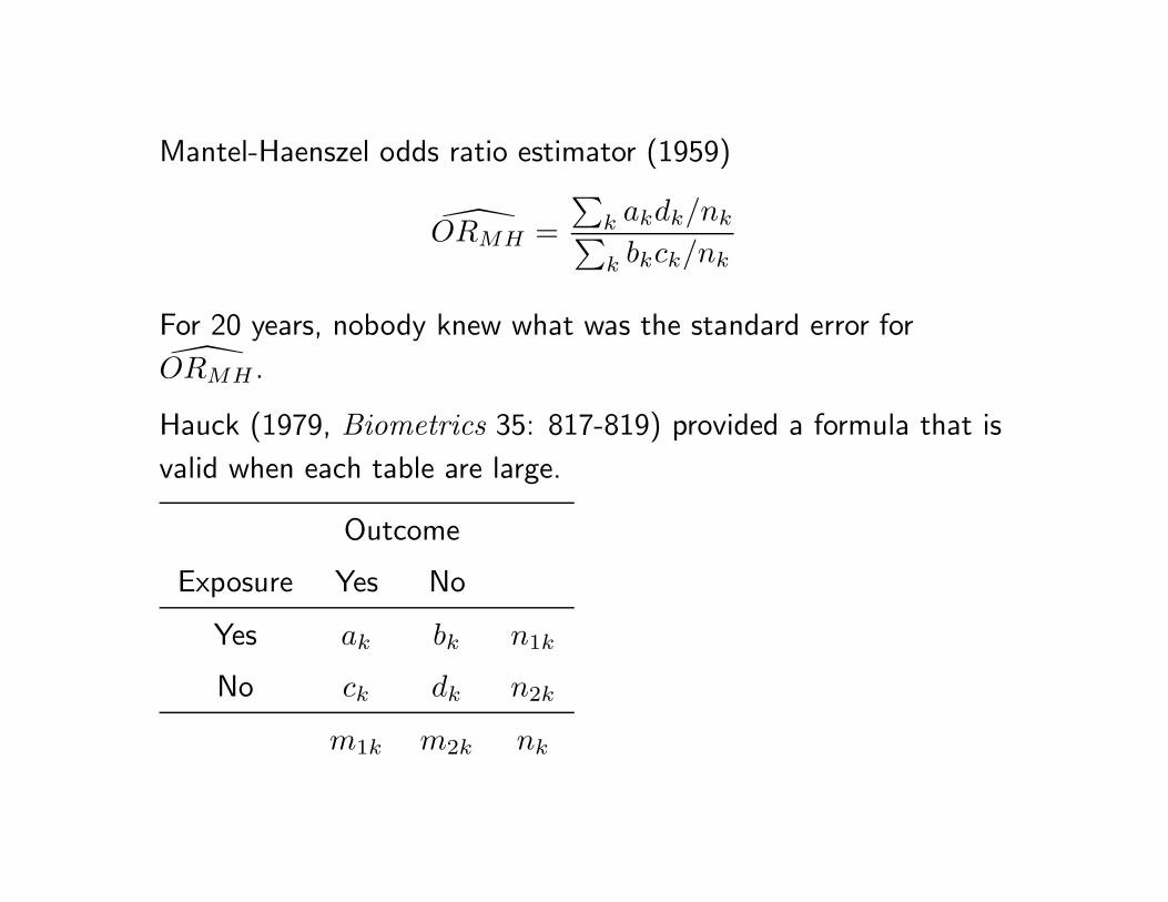
Mantel-Haenszel odds ratio estimator (1959)
ORMH =∑
k akdk/nk∑k bkck/nk
For 20 years, nobody knew what was the standard error forORMH .
Hauck (1979, Biometrics 35: 817-819) provided a formula that is
valid when each table are large.
Outcome
Exposure Yes No
Yes ak bk n1k
No ck dk n2k
m1k m2k nk
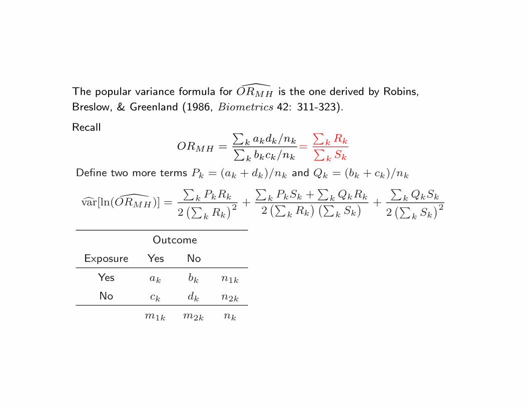
The popular variance formula for ORMH is the one derived by Robins,
Breslow, & Greenland (1986, Biometrics 42: 311-323).
Recall
ORMH =
∑k akdk/nk∑k bkck/nk
=
∑k Rk∑k Sk
Define two more terms Pk = (ak + dk)/nk and Qk = (bk + ck)/nk
var[ln( ORMH)] =
∑k PkRk
2(∑
k Rk
)2+
∑k PkSk +
∑k QkRk
2(∑
k Rk
) (∑k Sk
) +
∑k QkSk
2(∑
k Sk
)2
Outcome
Exposure Yes No
Yes ak bk n1k
No ck dk n2k
m1k m2k nk

(1 − α) × 100% CI for OR
exp[ln
(ORMH
)± Z1−α/2
√var[ln( ORMH)
]
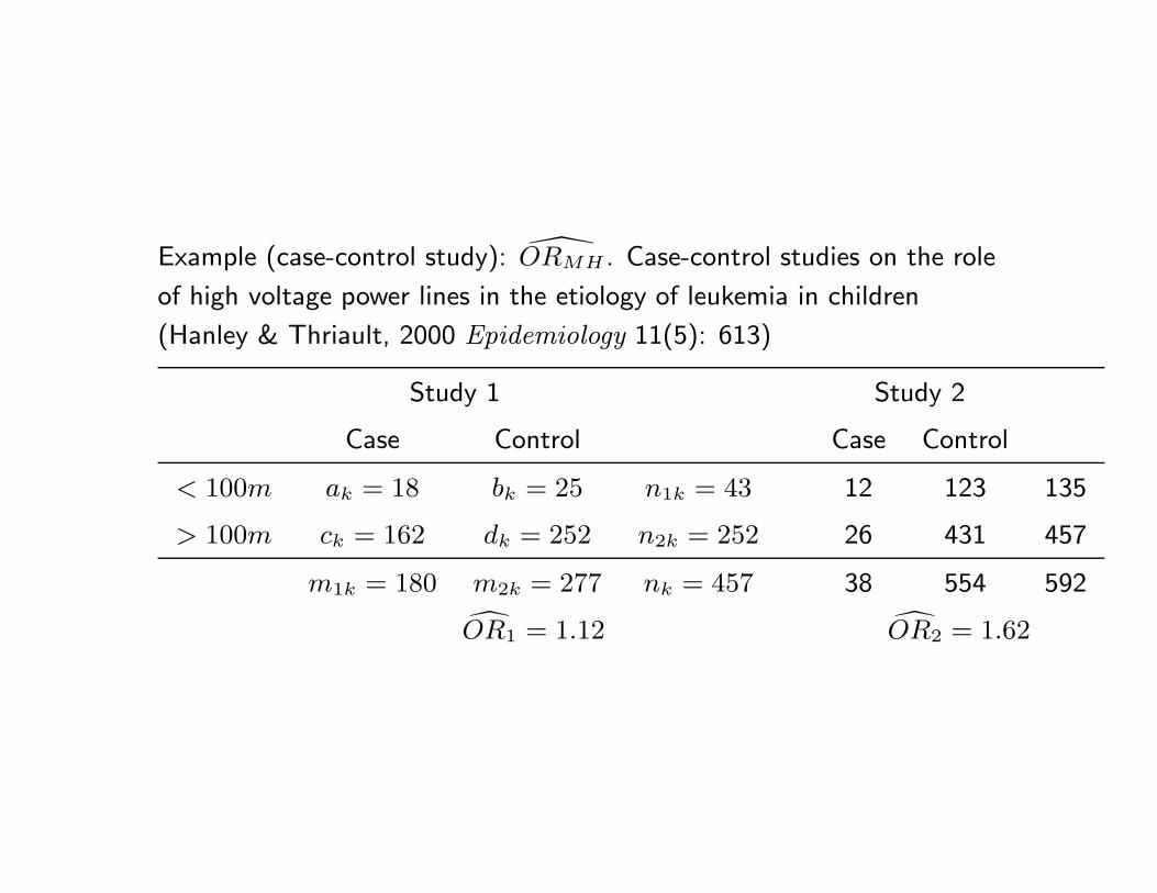
Example (case-control study): ORMH . Case-control studies on the role
of high voltage power lines in the etiology of leukemia in children
(Hanley & Thriault, 2000 Epidemiology 11(5): 613)
Study 1 Study 2
Case Control Case Control
< 100m ak = 18 bk = 25 n1k = 43 12 123 135
> 100m ck = 162 dk = 252 n2k = 252 26 431 457
m1k = 180 m2k = 277 nk = 457 38 554 592
OR1 = 1.12 OR2 = 1.62
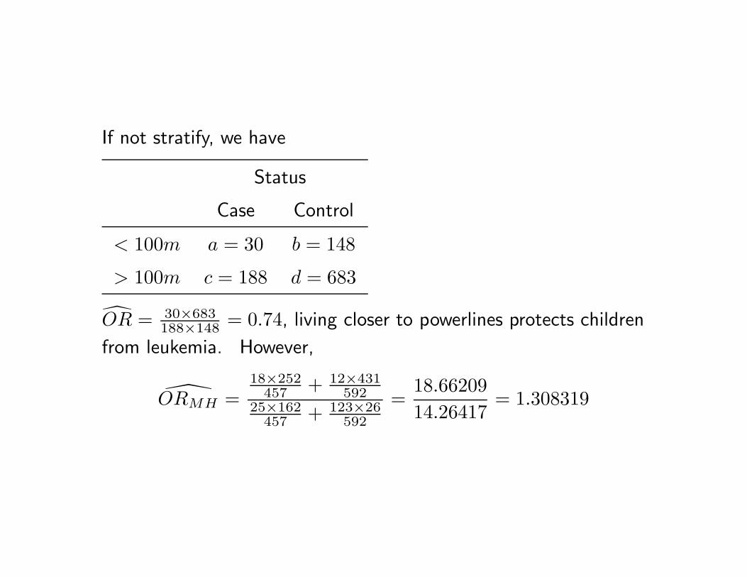
If not stratify, we have
Status
Case Control
< 100m a = 30 b = 148
> 100m c = 188 d = 683
OR = 30×683188×148 = 0.74, living closer to powerlines protects children
from leukemia. However,
ORMH =18×252
457 + 12×431592
25×162457 + 123×26
592
=18.6620914.26417
= 1.308319
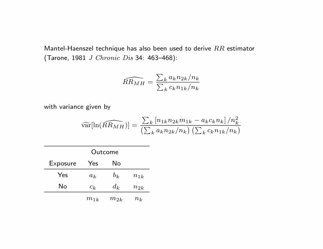
Mantel-Haenszel technique has also been used to derive RR estimator
(Tarone, 1981 J Chronic Dis 34: 463–468):
RRMH =
∑k akn2k/nk∑k ckn1k/nk
with variance given by
var[ln( RRMH)] =
∑k [n1kn2km1k − akcknk] /n2
k(∑k akn2k/nk
) (∑k ckn1k/nk
)
Outcome
Exposure Yes No
Yes ak bk n1k
No ck dk n2k
m1k m2k nk
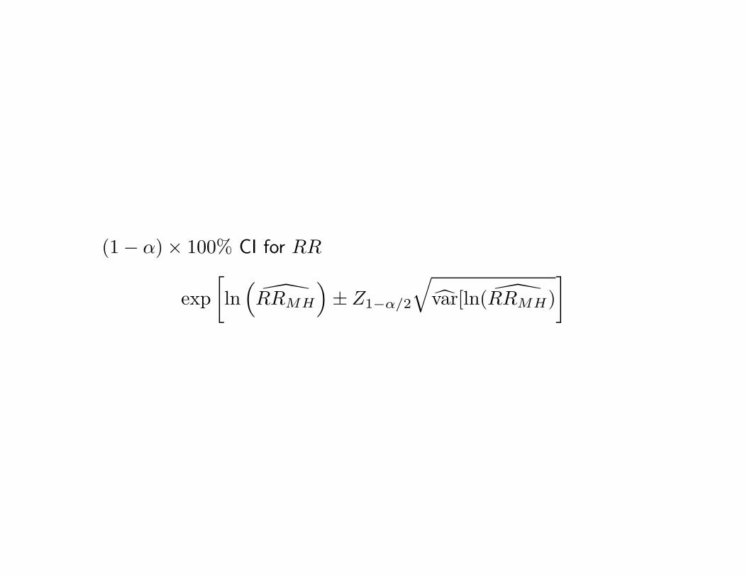
(1 − α) × 100% CI for RR
exp[ln
(RRMH
)± Z1−α/2
√var[ln( RRMH)
]
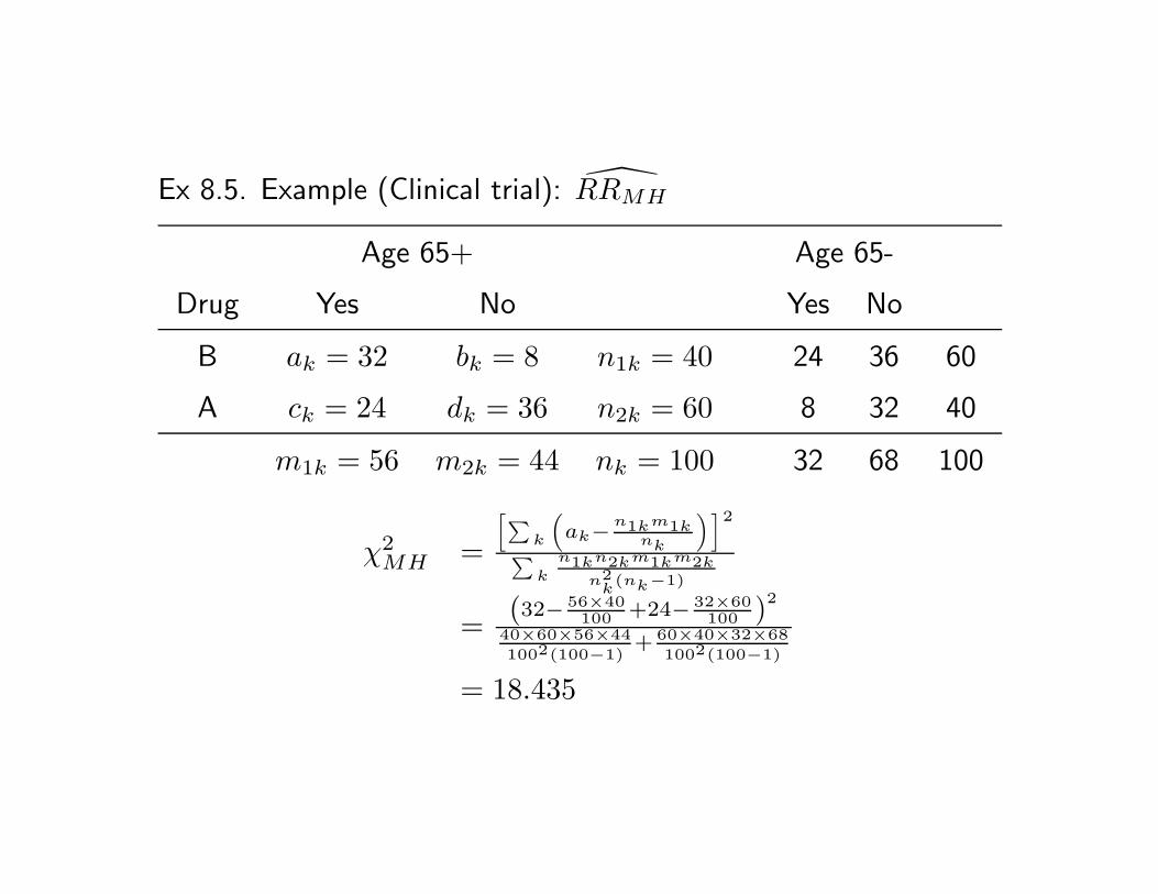
Ex 8.5. Example (Clinical trial): RRMH
Age 65+ Age 65-
Drug Yes No Yes No
B ak = 32 bk = 8 n1k = 40 24 36 60
A ck = 24 dk = 36 n2k = 60 8 32 40
m1k = 56 m2k = 44 nk = 100 32 68 100
χ2MH =
[∑k
(ak−n1km1k
nk
)]2
∑k
n1kn2km1km2kn2
k(nk−1)
= (32− 56×40100 +24− 32×60
100 )2
40×60×56×441002(100−1)
+ 60×40×32×681002(100−1)
= 18.435
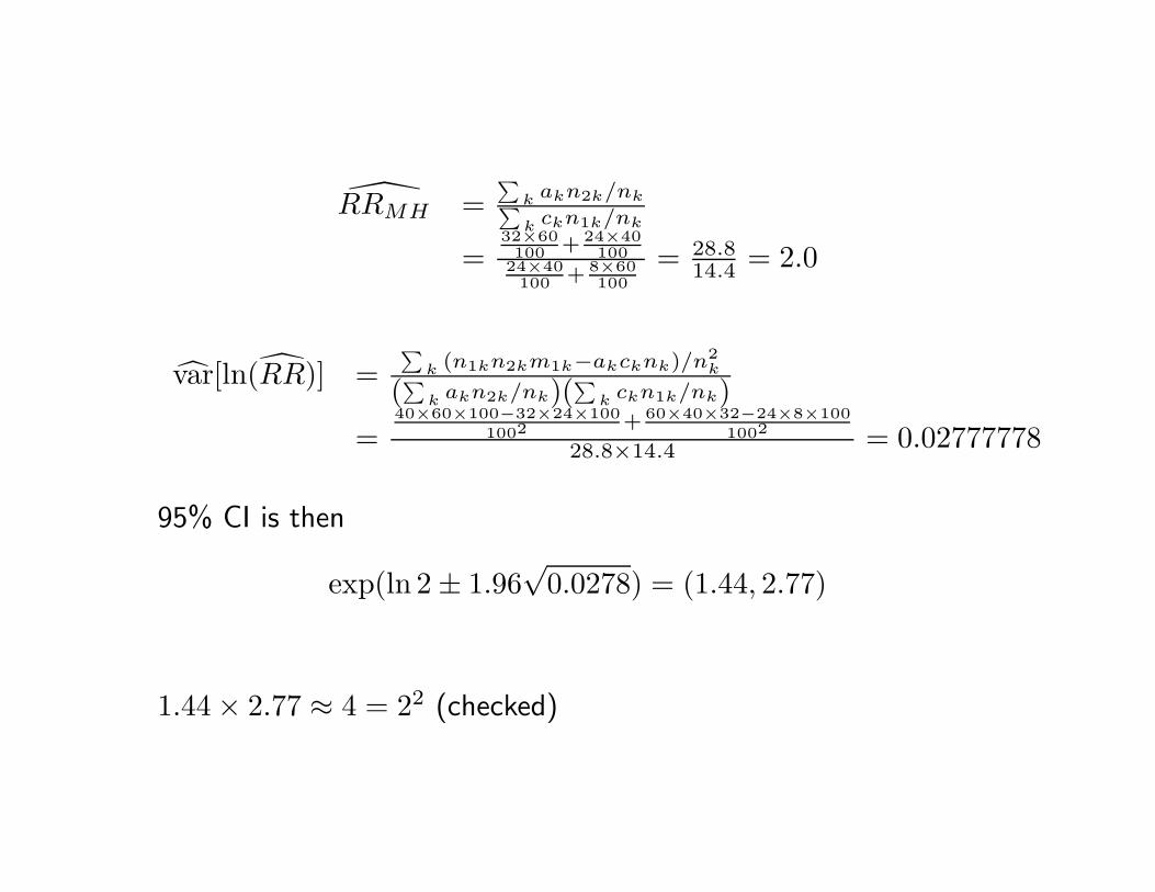
RRMH =∑
k akn2k/nk∑k ckn1k/nk
=32×60100 + 24×40
10024×40100 + 8×60
100= 28.8
14.4 = 2.0
var[ln(RR)] =∑
k (n1kn2km1k−akcknk)/n2k
(∑k akn2k/nk)(
∑k ckn1k/nk)
=40×60×100−32×24×100
1002+ 60×40×32−24×8×100
1002
28.8×14.4 = 0.02777778
95% CI is then
exp(ln 2 ± 1.96√
0.0278) = (1.44, 2.77)
1.44 × 2.77 ≈ 4 = 22 (checked)
Summary: Application of Mantel-Haenszel methods
Adjust for confounding (the original purpose): combat Simpson’s
paradox;
Meta-analysis: considering each study as a stratum.
The method of meta-analysis is commonly referred to as fix-effect
model with intention of summarizing available evidence, but not to
predict future study results. For that, random-effect model must
have to be adopted.
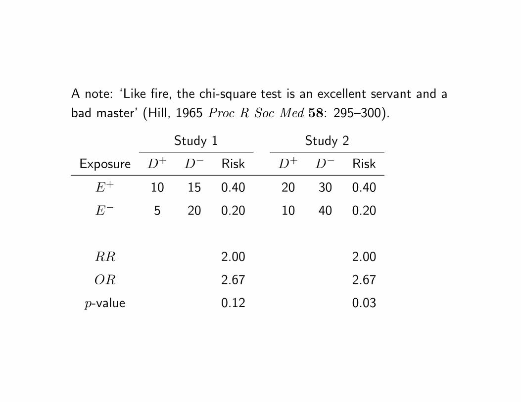
A note: ‘Like fire, the chi-square test is an excellent servant and a
bad master’ (Hill, 1965 Proc R Soc Med 58: 295–300).
Study 1 Study 2
Exposure D+ D− Risk D+ D− Risk
E+ 10 15 0.40 20 30 0.40
E− 5 20 0.20 10 40 0.20
RR 2.00 2.00
OR 2.67 2.67
p-value 0.12 0.03